Statistical theory of reversals in two-dimensional confined turbulent flows

Abstract

It is shown that the Truncated Euler Equations, i.e. a finite set of ordinary differential equations for the amplitude of the large-scale modes, can correctly describe the complex transitional dynamics that occur within the turbulent regime of a confined $2$D Navier-Stokes flow with bottom friction and a spatially periodic forcing. In particular, the random reversals of the large scale circulation on the turbulent background involve bifurcations of the probability distribution function of the large-scale circulation velocity that are described by the related microcanonical distribution which displays transitions from gaussian to bimodal and broken ergodicity. A minimal $13$-mode model reproduces these results.

The formation of large scale coherent structures is widely observed in atmospheric and oceanic flows and ascribed to the nearly bi-dimensional nature of these flows. Kraichnan showed that in two-dimensional (2D) turbulence, the energy is transferred from the forcing scale to larger scales due to the conservation of both energy and enstrophy by the inviscid dynamics Kraichnan (1967). In a confined flow domain and without large scale friction, the energy accumulates at the largest possible scale, thus generating coherent structures in the form of large scale vortices.

It has been observed in laboratory experiments that the large scale circulation generated by forcing a nearly $2$D flow at small scale can display random reversals Sommeria (1986). The large scale velocity has a bimodal probability density function (PDF) with two symmetric maxima related to the opposite signs of the large scale circulation. This regime bifurcates from another turbulent regime with a Gaussian velocity field with zero mean when the large scale friction is decreased. When the friction is decreased further, the reversals become less and less frequent and a condensed state with most of its kinetic energy in the large scale circulation is reached Herault et al. (2015). A similar sequence of transitions is observed in numerical simulations of the $2$D Navier-Stokes equation (NSE) with large scale friction and spatially periodic forcing Mishra et al. (2015).

These transitions correspond to bifurcations of a mean flow on a strongly turbulent background for which no theoretical tool exists so far. We show in this Letter that the truncated Euler equation (TEE), i.e. a finite set of ordinary differential equations (ODEs) for the amplitude of the large-scale modes without forcing and dissipation, can correctly describe these transitions. To wit, we compare the dynamical regimes observed in numerical simulations of the $2$D NSE with the ones obtained with the TEE when the characteristic scale $k_{c}^{-1}$ of the initial conditions is changed, with $k_{c}=\sqrt{\Omega/E}$ where $E$ is the kinetic energy of the flow and $\Omega$ is its enstrophy (integrated squared vorticity).

The dimensionless 2D NSE reads for an incompressible velocity field ${\bf u}=\nabla\times\psi$,

$$\frac{\partial\psi}{\partial t}-\frac{1}{\nabla^{2}}\{\psi,\nabla^{2}\psi\}=-\frac{1}{\rm Rh}\psi+\frac{1}{\rm Re}\nabla^{2}\psi+f_{\rm\psi}\,,$$ (1)

where $\psi(x,y,t)$ is the stream function and $\{f,g\}=\partial_{x}f\partial_{y}g-\partial_{x}g\partial_{y}f$ is the usual Poisson bracket. The first term on the right hand side represents the frictional force in the bottom boundary layer and $\nabla\times(f_{\rm\psi}\hat{\bf z})$ is the spatially periodic forcing, explicitly given by $f_{\rm\psi}=\frac{1}{144}\sin(6\,x)\sin(6\,y)$.

To model flow confinement we use free-slip boundary conditions; therefore, the stream-function can be Fourier expanded as

$$\psi(x,y)=\sum_{m,n}\hat{\psi}_{m,n}\sin(mx)\sin(ny).$$ (2)

The non-dimensional parameters are the Reynolds number, ${\rm Re}=UL/\nu$ and ${\rm Rh}=\tau U/L$, which represents the ratio of the inertial term to the friction on the bottom boundary. Here, $U$ is a characteristic large scale velocity, $L$ is the length of the square container, $\nu$ is the kinematic viscosity and $1/\tau$ is the damping rate related to the friction. The above equation has been made dimensionless using the length scale $L$ and the velocity scale $U$.

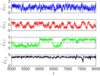
Figure 1: (Color online) Flow transitions: times series of $\hat{\psi}_{1,1}$ obtained from the DNS of the (a) Navier-Stokes equation (NSE) for different values of ${\rm Rh}$ and ${\rm Re}=5000/\pi^{2}$, (b) truncated-Euler equation (TEE) for different values of $k_{c}$. $\hat{\psi}_{1,1}^{NSE}$ and $\hat{\psi}_{1,1}^{TEE}$ have been divided by $10^{4}$ and $10^{2}$, respectively. (c) Plot of $k_{c}=\sqrt{\Omega/E}$ versus ${\rm Rh}$ from the DNS of NSE for two different Reynold’s numbers ${\rm Re}=3000/\pi^{2}$ (blue circles) and ${\rm Re}=5000/\pi^{2}$ (red crosses). Inset: Semilogy plots of the PDFs of $\hat{\psi}_{1,1}^{TEE}$ for different values of $k_{c}$. (d) Semilogy plots of the PDFs of $\hat{\psi}_{1,1}$ for different values of $k_{c}$ obtained from the finite-mode minimal model based on TEE; the lines on top of these PDFs indicate the estimation from our analytical method.

We perform direct numerical simulations (DNS) of Eq. (1), using standard pseudospectral methods Gottlieb and Orszag (1977) with $N_{c}^{2}$ collocation points and $2/3$ circular dealiasing: $k_{\rm max}=N_{c}/3$. Time stepping is performed with a second-order, exponential time differencing Runge-Kutta method Cox and Matthews (2002). DNSs of the NSE (1) are carried out for ${\rm Re}=3000/\pi^{2}$ and ${\rm Re}=5000/\pi^{2}$ with $N_{c}=256$. Very long time integration is needed to accumulate reliable statistics for the reversals, which become rare with increase in ${\rm Rh}$ (see below).

Direct time recordings of the amplitude of the lowest wave number mode of the stream function, $\hat{\psi}_{1,1}$, are displayed in Fig. 1(a) for ${\rm Re}=5000/\pi^{2}$ and different values of ${\rm Rh}$. For ${\rm Rh}=10$, the amplitude of the large scale circulation fluctuates around zero and its PDF is Gaussian (not shown). When ${\rm Rh}$ is increased, a first transition is observed within the turbulent regime and can be characterized by a change of the shape of the PDF that becomes bimodal. $\hat{\psi}_{1,1}$ fluctuates around two non zero most probable opposite values and displays random transitions between these two states (see Fig. 1(a2)). This corresponds to random reversals of the large scale circulation on a turbulent background. The mean waiting time between successive reversals increases with ${\rm Rh}$ (see Fig. 1(a3)) and finally a large scale circulation with a given sign becomes the dominant flow component (see Fig. 1(a4)). This is the condensed state described by Kraichnan Kraichnan (1967, 1975). The regime with random reversals of the large scale circulation is therefore located in parameter space between the condensed states and the turbulent regime with Gaussian velocity PDFs as observed in experiments Herault et al. (2015).

We now consider the approach, introduced by Lee Lee (1952) and developed by Kraichnan Kraichnan (1967, 1975) that relies on the 2D TEE. They showed that the Euler equation, truncated between a minimum and a maximum wave number, gives a set of ODEs for the amplitudes of the modes that follow a Liouville theorem Lee (1952). For 2D flows, the kinetic energy $E$ and the enstrophy $\Omega$ (integrated squared vorticity) are conserved; therefore, the Boltzmann-Gibbs canonical equilibrium distribution is of the form $\mathcal{P}=Z^{-1}\exp(-\alpha E-\beta\Omega)$, where $Z$ is the partition function and $\alpha$ and $\beta$ can be seen as inverse temperatures, determined by the total energy and enstrophy. Using this formalism, Kraichnan Kraichnan (1967, 1975) derived the absolute equilibria of the energy spectrum $E(k)$ and showed the existence of different regimes depending on the values of $\alpha$ and $\beta$. On the other hand, microcanonical distributions are defined by $\delta(E-E_{0})\delta(\Omega-\Omega_{0})$, where $E_{0}$ and $\Omega_{0}$ are respectively the energy and enstrophy of the initial conditions, and should be used to compute the PDFs in the reversal and condensed state (see below).

The TEE is obtained by performing a circular Galerkin truncation at wave-number $k_{\rm max}$ of the incompressible, Euler equation $\frac{\partial\psi}{\partial t}-\frac{1}{\nabla^{2}}\{\psi,\nabla^{2}\psi\}=0$, which is Eq. (1) without forcing or dissipation. The TEE in spectral space reads

$$\frac{\partial\psi_{\bf k}}{\partial t}=\frac{1}{k^{2}}\sum_{\bf p,q}({\bf p}\times{\bf q})q^{2}\psi_{\bf p}\psi_{\bf q}\delta_{{\bf k},{\bf p+q}}$$ (3)

with $\delta_{{\bf k},{\bf r}}$ the Kronecker delta and with Fourier modes satisfying $\psi_{\bf k}=0$ if $|{\bf k}|\geq k_{\rm max}$. Note that, because of the free-slip boundary conditions Eq. (2), the Fourier modes $\psi_{\bf k}$ are real numbers. This truncated system exactly conserves the quadratic invariants, energy and enstrophy, given in Fourier space by $E=\frac{1}{2}\sum_{\bf k}|{\bf u}_{\bf k}|^{2}$ and $\Omega=\frac{1}{2}\sum_{\bf k}k^{2}|{\bf u}_{\bf k}|^{2}$.

For TEE we take $k_{\rm max}$ as a free parameter and the same stream function expansion as that used for the NS Eq. (2), thus the numerical integration method is the same as the one described above for the NSE. In both cases, the minimum wavenumber is $k_{\rm min}=\sqrt{2}$. We use an initial velocity field with an energy spectra $E(k)=k/(\alpha+\beta k^{2})$, where by varying $\alpha$ and $\beta$ we can obtain different flow regimes in accordance with the Kraichnan’s absolute equilibrium predictions. We introduce a wave-number $k_{c}$ given by $k_{c}^{2}=\Omega/E$, which acts as an important control parameter of the system.

We next consider the results obtained using the TEE (3) with $k_{\rm max}=k_{f}$ (the NSE forcing wavenumber) and initial conditions with different values of $k_{c}$. Figure 1(b) shows the transitions between different turbulent regimes when $k_{c}$ is decreased. The corresponding PDFs of $\hat{\psi}_{1,1}$ obtained for different values of $k_{c}$ are displayed in the inset of Fig. 1(c). We observe the transition from Gaussian to bimodal PDF when $k_{c}$ is decreased and then the transition to the condensed regime with a given sign of the large scale circulation.

For NSE at large ${\rm Re}$, the effect of the large scale friction is to stop the inverse cascade before reaching the scale of the flow domain. ${\rm Rh}$ thus determines the largest scale of the flow that we can define using the wave number $k_{c}^{2}=\Omega/E$. $k_{c}$ is displayed in Fig. 1(c) for two values of ${\rm Re}$. It weakly depends on ${\rm Re}$ and monotonously decreases when ${\rm Rh}$ is increased. When ${\rm Rh}$ is large (small friction), the kinetic energy accumulates at the scale of the flow domain and the condensed state is obtained.

Although, we do not have a quantitative agreement between the transition values for $k_{c}$ for the TEE and ${\rm Rh}$ for the NSE when using the relation between $k_{c}$ and ${\rm Rh}$ displayed in Fig. 1(c), the same sequence of transitions is observed in both cases. Figure 1(d) shows that we keep this qualitative agreement when the truncation is lower, $k_{\rm max}=2\sqrt{5}$. This truncation leads to only $13$ ODEs for the amplitudes of the large scale modes (see Supplemental Material sup ). It is remarkable that this set of equations correctly describes the transitions observed between the different turbulent regimes observed in direct numerical simulations and experiments.

The TEE model (3) is a finite number of quadratic nonlinear ODEs for real variables $y_{i}$ (see the remark following Eq. (3) about the amplitudes of the Fourier modes noted $y_{i}$ hereafter to simplify the notations) that conserve both the energy $E(t)=\sum_{j=0}^{n}b_{E}(j)y_{j}^{2}$ and the enstrophy $\Omega(t)=\sum_{j=0}^{n}b_{\Omega}(j)y_{j}^{2}$ (see Supplemental Material sup ). By making use of the identities

$$\begin{split}&(2\pi)^{2}\delta(b_{E}y^{2}-E)\delta(b_{\Omega}y^{2}-\Omega)\\ &=\int_{-\infty}^{\infty}dp_{E}dp_{\Omega}e^{ip_{E}(b_{E}y^{2}-E)+ip_{\Omega}(b_{\Omega}y^{2}-\Omega)}\end{split}$$ (4)

and

$$\begin{split}\int_{-\infty}^{\infty}e^{i(p_{E}b_{E}+p_{\Omega}b_{\Omega})y^{2}}dy=\frac{\sqrt{\pi}}{\sqrt{-i(b_{E}p_{E}+b_{\Omega}p_{\Omega})}}\end{split}$$ (5)

we can write the total microcanonical phase space volume

$${\mathcal{V}}=\int\prod_{j=0}^{n}dy_{j}\delta\left(\sum_{j=0}^{n}b_{E}(j)y_{j}^{2}-E\right)\delta\left(\sum_{j=0}^{n}b_{\Omega}(j)y_{j}^{2}-\Omega\right)$$ (6)

as

$${\mathcal{V}}=\int_{-\infty}^{\infty}dp_{E}dp_{\Omega}e^{L_{\mathcal{V}}(p_{E},p_{\Omega})}$$ (7)

with

$$\begin{split}L_{\mathcal{V}}&=\sum_{j=0}^{n}\log\left(\frac{\sqrt{\pi}}{\sqrt{-i(p_{E}b_{E}(j)+p_{\Omega}b_{\Omega}(j))}}\right)\\ &+ip_{E}(-E)+ip_{\Omega}(-\Omega)-2\log(2\pi)\end{split}$$ (8)

Using the steepest descent method Zinn-Justin (2007); Bender and Orszag (1978) on the integral Eq. (7), the expression

$$\begin{split}{\mathcal{V}}(p_{E},p_{\Omega})=2\,\pi\,e^{L_{\mathcal{V}}}\Bigl{(}\det(\partial^{2}L_{\mathcal{V}}/\partial_{p_{E}}\partial_{p_{\Omega}})\Bigr{)}^{-1/2}\end{split}$$ (9)

furnishes an explicit parametric expression for ${\mathcal{V}}$ at the saddle-point $(p_{E},p_{\Omega})$ that corresponds to values of energy and enstrophy given by the saddle conditions

$$E(p_{E},p_{\Omega}) = i\sum_{j=0}^{n}\frac{b_{E}(j)}{2(p_{E}b_{E}(j)+p_{\Omega}b_{\Omega}(j))}$$

$$\Omega(p_{E},p_{\Omega}) = i\sum_{j=0}^{n}\frac{b_{\Omega}(j)}{2(p_{E}b_{E}(j)+p_{\Omega}b_{\Omega}(j))}$$ (10)

and thus to $k_{c}^{2}=\Omega/E$.

We can estimate the same way the phase space volume for a fixed value of $y_{0}$ by retracing the steps from Eq. (6) to (9), but with the product and sums going from $1$ to $n$ instead of $0$ to $n$. By combining these parametric representations, we obtain an explicit expression for the normalized PDF of $y_{0}$ that is shown in Fig.1(d) and displays a good agreement with the numerical results .

Note that canonical distributions with quadratic invariants are gaussian. When there is condensation of energy at large scale, only a few modes are present and then the canonical distribution has no reason to reproduce the microcanonical distribution results  Kells and Orszag (1978). Indeed, $k_{c}^{2}=\Omega/E<5$ with $\Omega=(1^{2}+1^{2})^{2}y_{0}^{2}+(1^{2}+2^{2})^{2}y_{1}^{2}+\dots$ and $E=(1^{2}+1^{2})y_{0}^{2}+(1^{2}+2^{2})y_{1}^{2}+\dots$ implies that $y_{0}\neq 0$. Thus the microcanonical PDF of $y_{0}$ has to obey $p(0)=0$ for $k_{c}^{2}<5$ which forbids reversals of the large scale circulation. This represents ergodicity breakdown. Our above results show that this breakdown is preceded by an ergodicity delay, in the sense that $p(0)$ becomes very small Dmitruk et al. (2014, 2011); Shebalin (1998).

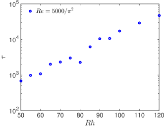
Figure 2: (Color online) Reversals: Semilogy plot of the mean waiting time $\tau$ between successive reversals versus ${\rm Rh}$, obtained from our DNSs of NSE for ${\rm Re}=5000/\pi^{2}$ (blue circles). Inset: Plot of the reversal frequency $1/\tau$ versus $k_{c}$ from the DNSs of TEE; it shows that the reversal frequency decreases linearly with $k_{c}$ with a critical $k_{c}^{*}\simeq 4.06$, below which the reversals are not observed for the integration time.

We now consider in more detail the regime with random reversals of the large scale circulation and its transition to the condensed regime for which the flow no longer explores the whole phase space, keeping a given sign of the large scale circulation. As shown above (compare Fig. 1(a) and (b)), the mean waiting time $\tau$ between successive reversals increases when ${\rm Rh}$ is increased in the NSE, respectively $k_{c}$ is decreased in the TEE. However, the divergence of $\tau$ does not follow the same law for the NSE and the TEE. Figure 2(a) shows an exponential increase of $\tau$ with ${\rm Rh}$ in the NSE, whereas a fit of the form $\tau\propto(k_{c}-k_{c}^{*})^{-1}$ with $k_{c}^{*}\simeq 4.06$ is observed in the TEE (see Fig. 2(b)). The later result is expected since there exists a critical value of $k_{c}$ below which reversals are not possible in order to fulfill the conservation of both $E$ and $\Omega$. We thus expect that $\tau$ becomes infinite for a finite value of $k_{c}$. A similar trend is not observed in the NSE for $\tau$ versus ${\rm Rh}$. This cannot be explained using the relation between $k_{c}$ and ${\rm Rh}$ displayed in Fig. 1(c) that is roughly linear close to the transition to the condensed regime. In contrast to the TEE, the NSE does not involve conserved quantities that prevent reversals, even when ${\rm Rh}$ is large. In addition, all the modes above $k_{f}$ that are suppressed in the TEE can act as an additional source of noise in the NSE and trigger reversals.

Although it can be expected that viscous dissipation is negligible for the dynamics of large scales, it is remarkable that taking into account the effect of large scale friction by selecting the value of $\Omega/E$ in the initial conditions of the TEE is enough to describe the bifurcations of the large scale flow using a small number of modes governed by the Euler equation. Thus, one discards the huge number of degrees of freedom related to small scale turbulent fluctuations. In addition, equilibrium statistical mechanics, using the microcanonical distribution related to the TEE, correctly describes the PDF of the large scale velocity in the different turbulent regimes. Transitions between different mean flows are widely observed in turbulent regimes, the most famous example being the drag crisis for which the wake of a sphere becomes narrower. Using the Navier-Stokes equation with noisy forcing Bouchet and Simonnet (2009) is a way to describe this type of transitions. The TEE as presented here, can provide a new method to describe the dynamics of large scales in turbulence and to model a bifurcation of the mean flow on a strongly turbulent background.

I Supplemental Material

We give here explicitly the set of thirteen ordinary differential equations (ODEs) for the amplitudes of the Fourier modes $\hat{\psi}_{m,n}$ that define the Truncated Euler Equation (TEE) in the case $k_{\rm max}=2\sqrt{5}$. Note that $\hat{\psi}_{m,n}$ are real numbers because of the free-slip boundary conditions (see text).

$$\begin{split}\frac{d\hat{\psi}_{11}}{dt}&=\frac{1}{2}\biggl{[}\bigl{(}2\hat{\psi}_{12}+5\hat{\psi}_{14}\bigr{)}\hat{\psi}_{23}+\hat{\psi}_{13}\bigl{(}2\hat{\psi}_{22}+5\hat{\psi}_{24}\bigr{)}\\ &-2\hat{\psi}_{22}\hat{\psi}_{31}-\hat{\psi}_{32}\bigl{(}2\hat{\psi}_{21}+5\hat{\psi}_{41}\bigr{)}\\ &+3\hat{\psi}_{33}\bigl{(}\hat{\psi}_{24}-\hat{\psi}_{42}\bigr{)}-5\hat{\psi}_{31}\hat{\psi}_{42}\biggr{]}\end{split}$$ (11)

$$\begin{split}\frac{d\hat{\psi}_{12}}{dt}&=\frac{1}{20}\biggl{[}25\hat{\psi}_{13}\hat{\psi}_{21}+54\hat{\psi}_{14}\hat{\psi}_{22}\\ &+\hat{\psi}_{11}\bigl{(}9\hat{\psi}_{21}-11\hat{\psi}_{23}\bigr{)}+25\hat{\psi}_{21}\hat{\psi}_{31}\\ &+21\hat{\psi}_{23}\hat{\psi}_{31}+56\hat{\psi}_{24}\hat{\psi}_{32}-39\hat{\psi}_{21}\hat{\psi}_{33}\\ &+49\hat{\psi}_{31}\hat{\psi}_{41}+9\hat{\psi}_{33}\hat{\psi}_{41}\biggr{]}\end{split}$$ (12)

$$\begin{split}\frac{d\hat{\psi}_{21}}{dt}&=\frac{1}{20}\biggl{[}-49\hat{\psi}_{13}\hat{\psi}_{14}-\hat{\psi}_{11}\bigl{(}9\hat{\psi}_{12}-11\hat{\psi}_{32}\bigr{)}\\ &-21\hat{\psi}_{13}\hat{\psi}_{32}-\hat{\psi}_{12}\bigl{(}25\hat{\psi}_{13}+25\hat{\psi}_{31}-39\hat{\psi}_{33}\bigr{)}\\ &-9\hat{\psi}_{14}\hat{\psi}_{33}-54\hat{\psi}_{22}\hat{\psi}_{41}-56\hat{\psi}_{23}\hat{\psi}_{42}\biggr{]}\end{split}$$ (13)

$$\begin{split}\frac{d\hat{\psi}_{22}}{dt}&=\frac{1}{4}\biggl{[}-9\hat{\psi}_{12}\hat{\psi}_{14}-4\hat{\psi}_{11}\bigl{(}\hat{\psi}_{13}-\hat{\psi}_{31}\bigr{)}\\ &+5\hat{\psi}_{14}\hat{\psi}_{32}+9\hat{\psi}_{21}\hat{\psi}_{41}-5\hat{\psi}_{23}\hat{\psi}_{41}\biggr{]}\end{split}$$ (14)

$$\begin{split}\frac{d\hat{\psi}_{13}}{dt}&=\frac{1}{10}\biggl{[}\hat{\psi}_{11}(6\hat{\psi}_{22}-9\hat{\psi}_{24})+7\hat{\psi}_{21}\bigl{(}3\hat{\psi}_{14}+2\hat{\psi}_{32}\bigr{)}\\ &+11\hat{\psi}_{32}\hat{\psi}_{41}+\hat{\psi}_{31}\bigl{(}4\hat{\psi}_{22}+25(\hat{\psi}_{24}+\hat{\psi}_{42})\bigr{)}\biggr{]}\end{split}$$ (15)

$$\begin{split}\frac{d\hat{\psi}_{31}}{dt}&=\frac{1}{10}\biggl{[}-14\hat{\psi}_{12}\hat{\psi}_{23}-11\hat{\psi}_{14}\hat{\psi}_{23}-21\hat{\psi}_{12}\hat{\psi}_{41}\\ &-\hat{\psi}_{11}\bigl{(}6\hat{\psi}_{22}-9\hat{\psi}_{42}\bigr{)}\\ &-\hat{\psi}_{13}\bigl{(}4\hat{\psi}_{22}+25(\hat{\psi}_{24}+\hat{\psi}_{42})\bigr{)}\biggr{]}\end{split}$$ (16)

$$\begin{split}\frac{d\hat{\psi}_{23}}{dt}&=\frac{1}{52}\biggl{[}35\hat{\psi}_{12}\hat{\psi}_{31}+77\hat{\psi}_{14}\hat{\psi}_{31}\\ &+\hat{\psi}_{11}\bigl{(}3\hat{\psi}_{12}-75\hat{\psi}_{14}+55\hat{\psi}_{32}\bigr{)}\\ &+90\hat{\psi}_{22}\hat{\psi}_{41}+42\hat{\psi}_{24}\hat{\psi}_{41}+120\hat{\psi}_{21}\hat{\psi}_{42}\biggr{]}\end{split}$$ (17)

$$\begin{split}\frac{d\hat{\psi}_{32}}{dt}&=\frac{1}{52}\biggl{[}-\hat{\psi}_{11}\bigl{(}3\hat{\psi}_{21}+55\hat{\psi}_{23}-75\hat{\psi}_{41}\bigr{)}\\ &-7\hat{\psi}_{13}\bigl{(}5\hat{\psi}_{21}+11\hat{\psi}_{41}\bigr{)}\\ &-6\bigl{(}20\hat{\psi}_{12}\hat{\psi}_{24}+\hat{\psi}_{14}(15\hat{\psi}_{22}+7\hat{\psi}_{42})\bigr{)}\biggr{]}\end{split}$$ (18)

$$\begin{split}\frac{d\hat{\psi}_{14}}{dt}&=\frac{1}{68}\biggl{[}-35\hat{\psi}_{13}\hat{\psi}_{21}+18\hat{\psi}_{12}\hat{\psi}_{22}+55\hat{\psi}_{11}\hat{\psi}_{23}\\ &-33\hat{\psi}_{23}\hat{\psi}_{31}+50\hat{\psi}_{22}\hat{\psi}_{32}\\ &+117\hat{\psi}_{21}\hat{\psi}_{33}-15\hat{\psi}_{33}\hat{\psi}_{41}+98\hat{\psi}_{32}\hat{\psi}_{42}\biggr{]}\end{split}$$ (19)

$$\begin{split}\frac{d\hat{\psi}_{41}}{dt}&=\frac{1}{68}\biggl{[}-18\hat{\psi}_{21}\hat{\psi}_{22}-50\hat{\psi}_{22}\hat{\psi}_{23}-98\hat{\psi}_{23}\hat{\psi}_{24}\\ &+35\hat{\psi}_{12}\hat{\psi}_{31}-55\hat{\psi}_{11}\hat{\psi}_{32}\\ &+33\hat{\psi}_{13}\hat{\psi}_{32}-117\hat{\psi}_{12}\hat{\psi}_{33}+15\hat{\psi}_{14}\hat{\psi}_{33}\biggr{]}\end{split}$$ (20)

$$\begin{split}\frac{d\hat{\psi}_{24}}{dt}&=\frac{1}{10}\biggl{[}8\hat{\psi}_{12}\hat{\psi}_{32}+2\hat{\psi}_{11}\bigl{(}\hat{\psi}_{13}+6\hat{\psi}_{33}\bigr{)}\\ &+7\hat{\psi}_{23}\hat{\psi}_{41}+18\hat{\psi}_{22}\hat{\psi}_{42}\biggr{]}\end{split}$$ (21)

$$\begin{split}\frac{d\hat{\psi}_{42}}{dt}&=\frac{1}{10}\biggl{[}-8\hat{\psi}_{21}\hat{\psi}_{23}-18\hat{\psi}_{22}\hat{\psi}_{24}-2\hat{\psi}_{11}\hat{\psi}_{31}\\ &-7\hat{\psi}_{14}\hat{\psi}_{32}-12\hat{\psi}_{11}\hat{\psi}_{33}\biggr{]}\end{split}$$ (22)

$$\begin{split}\frac{d\hat{\psi}_{33}}{dt}&=-\frac{3}{2}\biggl{[}\hat{\psi}_{14}\hat{\psi}_{21}-\hat{\psi}_{12}\hat{\psi}_{41}\\ &+\hat{\psi}_{11}\bigl{(}\hat{\psi}_{24}-\hat{\psi}_{42}\bigr{)}\biggr{]}\end{split}$$ (23)

The dynamical evolution of the above set of ODEs conserves the total energy and enstrophy, which are given by

$$\begin{split}E&=(1^{2}+1^{2})\hat{\psi}_{11}^{2}+(1^{2}+2^{2})\hat{\psi}_{12}^{2}+(2^{2}+1^{2})\hat{\psi}_{21}^{2}\\ &+(2^{2}+2^{2})\hat{\psi}_{22}^{2}+(3^{2}+1^{2})\hat{\psi}_{31}^{2}+(1^{2}+3^{2})\hat{\psi}_{13}^{2}\\ &+(2^{2}+3^{2})\hat{\psi}_{23}^{2}+(3^{2}+2^{2})\hat{\psi}_{32}^{2}+(1^{2}+4^{2})\hat{\psi}_{14}^{2}\\ &+(4^{2}+1^{2})\hat{\psi}_{41}^{2}+(2^{2}+4^{2})\hat{\psi}_{24}^{2}+(4^{2}+2^{2})\hat{\psi}_{42}^{2}\\ &+(3^{2}+3^{2})\hat{\psi}_{33}^{2},\end{split}$$ (24)

and

$$\begin{split}\Omega&=(1^{2}+1^{2})^{2}\hat{\psi}_{11}^{2}+(1^{2}+2^{2})^{2}\hat{\psi}_{12}^{2}+(2^{2}+1^{2})^{2}\hat{\psi}_{21}^{2}\\ &+(2^{2}+2^{2})^{2}\hat{\psi}_{22}^{2}+(3^{2}+1^{2})^{2}\hat{\psi}_{31}^{2}+(1^{2}+3^{2})^{2}\hat{\psi}_{13}^{2}\\ &+(2^{2}+3^{2})^{2}\hat{\psi}_{23}^{2}+(3^{2}+2^{2})^{2}\hat{\psi}_{32}^{2}+(1^{2}+4^{2})^{2}\hat{\psi}_{14}^{2}\\ &+(4^{2}+1^{2})^{2}\hat{\psi}_{41}^{2}+(2^{2}+4^{2})^{2}\hat{\psi}_{24}^{2}+(4^{2}+2^{2})^{2}\hat{\psi}_{42}^{2}\\ &+(3^{2}+3^{2})^{2}\hat{\psi}_{33}^{2}.\end{split}$$ (25)

References

• Kraichnan (1967) R. H. Kraichnan, Physics of Fluids 10, 1417 (1967).
• Sommeria (1986) J. Sommeria, Journal of Fluid Mechanics 170, 139 (1986).
• Herault et al. (2015) J. Herault, F. Pétrélis,  and S. Fauve, EPL (Europhysics Letters) 111, 44002 (2015).
• Mishra et al. (2015) P. K. Mishra, J. Herault, S. Fauve,  and M. K. Verma, Phys. Rev. E 91, 053005 (2015).
• Gottlieb and Orszag (1977) D. Gottlieb and S. A. Orszag, Numerical Analysis of Spectral Methods (SIAM, Philadelphia, 1977).
• Cox and Matthews (2002) S. M. Cox and P. C. Matthews, J. Comput. Phys. 176, 430 (2002).
• Kraichnan (1975) R. H. Kraichnan, Journal of Fluid Mechanics 67, 155 (1975).
• Lee (1952) T. D. Lee, Quart Appl Math 10, 69 (1952).
• (9) See Supplemental Material at for the additional details.
• Zinn-Justin (2007) J. Zinn-Justin, Phase Transitions and Renormalization Group (Oxford University Press, 2007).
• Bender and Orszag (1978) C. M. Bender and S. A. Orszag, Advanced mathematical methods for scientists and engineers, International series in pure and applied mathematics (McGraw-Hill Book Company, Auckland, Bogota, Paris, 1978).
• Note (1) Purely imaginary values for $(p_{E},p_{\Omega})$ parametrize real values of $(E,\Omega)$).
• Note (2) We have checked (data not shown) that the steepest-descent estimates correctly represent microcanonical Monte-Carlo results, even in the highly bimodal regime.
• Kells and Orszag (1978) L. C. Kells and S. A. Orszag, Physics of Fluids 21, 162 (1978).
• Dmitruk et al. (2014) P. Dmitruk, P. D. Mininni, A. Pouquet, S. Servidio,  and W. H. Matthaeus, Phys. Rev. E 90, 043010 (2014).
• Dmitruk et al. (2011) P. Dmitruk, P. D. Mininni, A. Pouquet, S. Servidio,  and W. H. Matthaeus, Phys. Rev. E 83, 066318 (2011).
• Shebalin (1998) J. V. Shebalin, Physics Letters A 250, 319 (1998).
• Bouchet and Simonnet (2009) F. Bouchet and E. Simonnet, Phys. Rev. Lett. 102, 094504 (2009).