An Application of the EM-algorithm to Approximate Empirical Distributions of Financial Indices with the Gaussian Mixtures

Abstract

In this study I briefly illustrate application of the Gaussian mixtures to approximate empirical distributions of financial indices (DAX, Dow Jones, Nikkei, RTSI, S$\&$P 500). The resulting distributions illustrate very high quality of approximation as evaluated by Kolmogorov-Smirnov test. This implies further study of application of the Gaussian mixtures to approximate empirical distributions of financial indices.

financial indices, Gaussian distribution, mixtures of Gaussian distributions, Gaussian mixtures, EM-algorithm

1 Introduction

Approximation of empirical distributions of financial indices using mixture of Gaussian distributinos (Gaussian mixtures) (eq. (1)) has been recently discussed by Tarasenko and Artukhov [1]. Here I provide detailed explanation of steps and methods.

$$GM=\sum^{n}_{i=1}{p_{i}\cdot N(\mu_{i},\sigma_{i})}$$ (1)

2 EM-algorithm for mixture separation

2.1 General Theory

The effective procedure for separation of mixtures was proposed by Day [2, 3] and Dempster et al. [4]. This procedure is based on maximization of logarithmic likelihood function under parameters $p_{1}$,$p_{2}$,…, $p_{k-1}$,$\Theta_{1}$,$\Theta_{2}$,…, $\Theta_{k}$, where $k$ is number of mixture components:

$$\sum_{i=1}^{n}{}ln\bigg{(}\sum_{j=1}^{k}{p_{j}\cdot f(x_{i};\Theta_{j})}\bigg{)}\to\max_{p_{j},\Theta_{j}}$$ (2)

In general, the algorithms of mixture separations based on (2) are called Estimation and Maximization (EM) algorithms. EM-algorithm consists of two steps: E - expectation and M-maximization. This section is focused scheme how to construct EM-algorithm.

Let $g_{ij}$ is defined as posterior porbability of oservations $x_{i}$ to belong to $j$-th mixture component (class):

$$g_{ij}=\frac{p_{j}\cdot f(x_{i};\Theta_{j})}{\sum_{j=1}^{k}{p_{j}\cdot f(x_{i};\Theta_{j})}}$$ (3)

Posterior probability $g_{ij}$ is equal or greater then 0 and $\sum_{j=1}^{k}{g_{ij}}$ for any $i$.

Let $\Theta$ be a vector of parameters: $\Theta$ = ($p_{1}$,$p_{2}$,…, $p_{k-1}$,$\Theta_{1}$,$\Theta_{2}$,…, $\Theta_{k}$). Next, we deompose the logarithms likelihood function into three components:

$$lnL(\Theta)=\sum_{i=1}^{n}{}ln\bigg{(}\sum_{j=1}^{k}{p_{j}\cdot f(x_{i};\Theta_{j})}\bigg{)}=$$ (4)

$$\sum_{j=1}^{k}{\sum_{i=1}^{n}{g_{ij}ln(p_{j})}}$$ (5)

$$+\sum_{j=1}^{k}{\sum_{i=1}^{n}{g_{ij}lnf(x_{i};\Theta_{j})}}$$ (6)

$$-\sum_{j=1}^{k}{\sum_{i=1}^{n}{g_{ij}ln(g_{ij})}}$$ (7)

For this algorithm to work, the initial value $\hat{\Theta}^{0}$ is used to calculate inital approximations for posterior probabilities $g^{0}_{ij}$. This is Expectation step. Then values of $g^{0}_{ij}$ are used to calculate value of $\hat{\Theta}^{1}$ during the Maximization step.

Each of components (6) and (7) are maximized independently from each other. This is possible because component (6) depends only on $p_{j}$ ($i$=1,…,$k$), and component (7) depends only on $\Theta_{j}$ ($j$=1,…,$n$).

As a solution of optimization task (8)

$$\sum_{j=1}^{k}{\sum_{i=1}^{n}{g_{ij}ln(p_{j})}}\to\max_{p_{1},...,p_{k}}$$ (8)

a value of $p^{(t+1)}_{j}$ for the iteration $t+1$ is calculated as:

$$p^{(t+1)}_{j}=\frac{1}{n}\sum_{i=1}^{n}{g^{(t)}_{ij}}$$ (9)

where $t$ is iteration number, $t$ = 1,2, ,,,

A solution of optimization task (10)

$$\sum_{j=1}^{k}{\sum_{i=1}^{n}{g_{ij}lnf(x_{i};\Theta_{j})}}\to\max_{\Theta_{1},...,\Theta_{k}}$$ (10)

depends on a particular type of function $f(\cdot)$.

Next we consider solution of optimization task (10), when $f(\cdot)$ is Gaussian distribution.

2.2 Mixtures of Gaussian Distributions

Here we employ Guassian distributions:

$$N(x;\mu,\sigma)=\frac{1}{\sigma\sqrt{2\pi}}exp^{-\frac{(x-\mu)^{2}}{2\sigma^{2}}}$$ (11)

Therefore, a specific formula to compute posterior probabilities in the case of Gaussian mixtures is

$$g_{ij}=\frac{exp^{-\frac{(x-\mu)^{2}}{2\sigma^{2}}+ln(p_{j})-ln(\sigma_{j})}}{\sum_{j=1}^{k}{exp^{-\frac{(x-\mu)^{2}}{2\sigma^{2}}+ln(p_{j})-ln(\sigma_{j})}}}$$ (12)

According to the EM-algorithm, the task is to find value of parameters $\Theta_{j}$ = $(\mu_{j},\sigma_{j})$ by solving maximization problem (14)

$$\sum_{j=1}^{k}{lnL_{j}}=\sum_{j=1}^{k}{\sum_{i=1}^{n}{lnL_{j}}}=$$ (13)

$$\sum_{j=1}^{k}{\sum_{i=1}^{n}{ln\bigg{(}\frac{1}{\sigma\sqrt{2\pi}}exp^{-\frac{(x-\mu)^{2}}{2\sigma^{2}}}\bigg{)}}}\to\max_{\Theta_{1},\Theta_{2},...,\Theta_{k}}$$ (14)

The solution of this mazimization problem is given by eqs. (16) and (16):

$$\hat{\mu}_{j}=\frac{1}{\sum_{i=1}^{n}{g_{ij}}}\sum_{i=1}^{n}{g_{ij}x_{i}}$$ (15)

$$\hat{\sigma}_{j}=\frac{1}{\sum_{i=1}^{n}{g_{ij}}}\sum_{i=1}^{n}{g_{ij}(x_{i}-\hat{\mu}_{j})^{2}}$$ (16)

Having calculated optimal values for weights $p_{j}$ and paramaters $\Theta_{j}$ ($j$=1,…,$k$) during a single iteration, we apply these optimal values to obtain estimates of posterior probabilities during the Expectation step of the next iteration.

As a stop criterion, we use difference between values of loglikelyhood on iteration $t$ and iteration $t+1$:

$$lnL^{(t+1)}(\Theta)-lnL^{(t)}(\Theta)<\epsilon$$ (17)

where $\epsilon$ is infinitely small real value.

3 An Application of the EM-algorithm to Approximate Empirical Distributions of Financial Indices with Guassian Mixtures

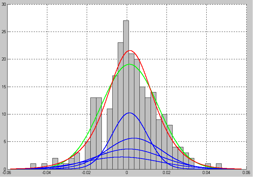
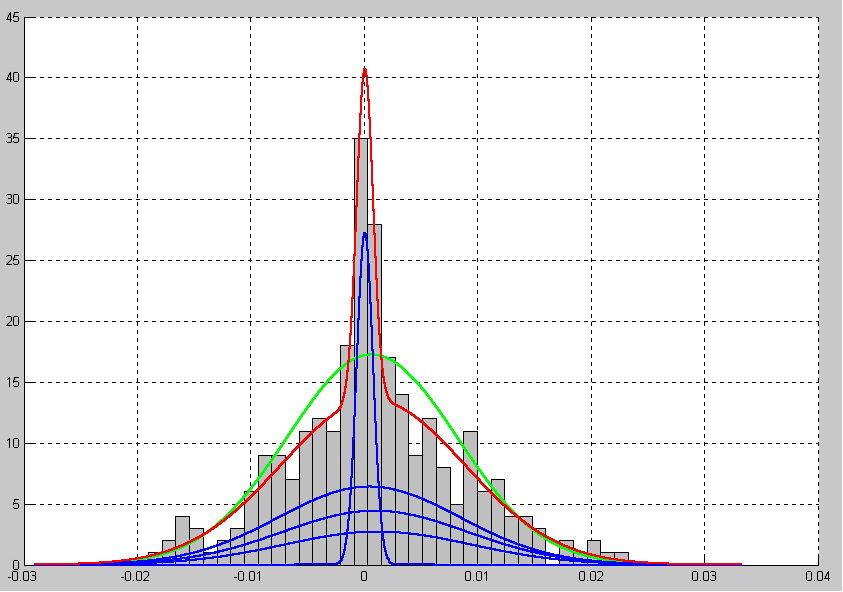
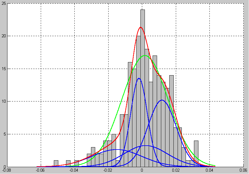
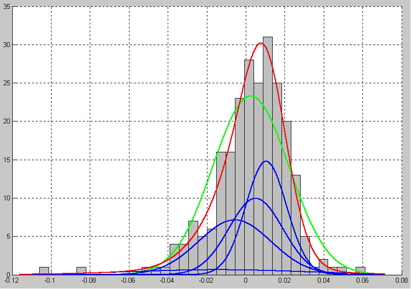
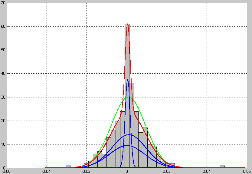
In this section, I provide several examples of EM-algorithm applications to approximate empirical distributions of financial indices with Gaussian mixtures. I consider the following indices: DAX, Dow Jones Industrial, Nikkei, RTSI, and S$\&$P 500.

In Figs. 1-5, the green line corresponds to the Gaussian distribution, the red line illustrates a Gaussian mixture and the blue lines represent components of the Gaussian mixture.

Table 1: Mixture model for DAX

	Weight	Mean	Standard
			Diviation
Component 1	0.152	-0.002	0.018
Component 2	0.223	0.001	0.017
Component 3	0.287	0.004	0.014
Component 4	0.337	0.001	0.009

Figure 1: Empirical distribution of DAX values during the period 14 April 2003 - 14 April 2004. p $<$ 0.05, KSSTAT=0.031

Table 2: Mixture model for Dow Jones (DJIA)

	Weight	Mean	Standard
			Diviation
Component 1	0.173	0.001	0.008
Component 2	0.279	0.001	0.008
Component 3	0.396	0.001	0.008
Component 4	0.152	0.000	0.001

Figure 2: Empirical distribution of Dow Jones Industrial values during the period 14 April 2003 - 14 April 2004, p $<$ 0.01, KSSTAT=0.023

Table 3: Mixture model for Nikkei

	Weight	Mean	Standard
			Diviation
Component 1	0.167	-0.014	0.014
Component 2	0.180	0.002	0.013
Component 3	0.367	0.011	0.008
Component 4	0.286	-0.002	0.005

Figure 3: Empirical distribution of Nikkei index values during the period 14 April 2003 - 14 April 2004, p $<$ 0.01, KSSTAT=0.027

Table 4: Mixture model for RTSI

	Weight	Mean	Standard
			Diviation
Component 1	0.062	-0.014	0.044
Component 2	0.294	-0.005	0.019
Component 3	0.303	0.005	0.014
Component 4	0.341	0.011	0.011

Figure 4: Empirical distribution of RTSI values during the period 14 April 2003 - 14 April 2004, p $<$ 0.01, KSSTAT=0.021

Table 5: Mixture model for S$\&$P 500

	Weight	Mean	Standard
			Diviation
Component 1	0.014	0.011	0.027
Component 2	0.331	0.000	0.009
Component 3	0.470	0.001	0.009
Component 4	0.186	0.000	0.001

Figure 5: Empirical distribution of S$\&$P 500 values during the period 14 April 2003 - 14 April 2004, p $<$ 0.01, KSSTAT=0.024

4 Discussion and Conclusion

The results presented in this study illustrate that EM-algrothim can be effectively used to approximate empiral distributions of log daily differences of financial indices. Throughout the data for five selected indices, EM-algorithm provided very good approximation of empoiral distirbution with Gaussian mixtures.

The approximations based on Gaussian mixtures can be used to improve application of Value-at-Risk and other methods for financial risk analysis.

This implies further explorations in applying Gaussian mixtures and the EM-algorithm for the purpose of approximation of empirial distirbutions of financial indices.

References

- [1] Tarasenko, S., and Artukhov, S. (2004) Stock market pricing models. In the Proceedings of International Conference of Young Scientists Lomonosov 2004, p. 248-250.
- [2] Day, N.E. (1969) Divisive cluster analysis and test for multivariate normality. Session of the ISI, London, 1969.
- [3] Day, N.E. (1969) Estimating the components of a mixture of normal distributions., Biometrika, 56, N3.
- [4] Dempster, A., Laird, G. and Rubin, J. (1977) Maximum likelihood from incomplete data via EM algorithm. Journal of Royal Statistical Society, B, 39.