Abstract

The discretization of the density matrix is proposed as a nonlinear positive map for systems with continuous variables. This procedure is used to calculate the entanglement between two modes through different criteria, such as Tsallis entropy, von Neumann entropy and linear entropy and the logarithmic negativity. As an example, we study the dynamics of entanglement for the two-mode squeezed vacuum state in the parametric amplifier and show good agreement with the analytic results. The loss of information on the system state due to the discretization of the density matrix is also addressed.

Keywords: Non linear positive maps, entanglement, entropies, logarithmic negativity.

1 Introduction

The pure state of a quantum system is identified with the wave function [1], while its mixed state is identified with the density matrix [2, 3, 4]. The time evolution of the quantum-system state provides the transformation (map) of the initial-state density matrix $\rho(0)$ onto the density matrix at time $t$, i.e., $\rho(0)\to\rho(t)$. The density matrix has nonnegative eigenvalues only, and such transformations are called positive maps. Among the positive maps, there are linear positive maps and nonlinear ones. The set of linear positive maps contains a subset of completely positive maps. The properties of the maps were considered in [5, 6, 7], and nonlinear maps were discussed in [8, 9].

A positive map is a transformation of a density matrix into a density matrix, i.e., this kind of operation preserves the trace of the density matrix, its hermiticity and positivity. Any quantum operation can be expressed as a positive map. In particular, the study of completely positive maps have been of great interest in the quantum information theory; it provides the result that the transmission of classical or quantum information can be represented by a set of operators defining a completely positive map, also called the quantum channel.

There exist different capacities of a system to transmit information: the classical capacity [10], the quantum capacity [11], and the entangled assisted capacity [12, 13]. Some of these capacities can be calculated through the three von Neumann entropies, such as the entropy of the input system state $\rho$, the entropy associated to the map $\Phi(\rho)$, and the entropy exchange $(\Phi\otimes\textrm{Id})|\psi\rangle\langle\psi|$, where $|\psi\rangle$ denotes the state which, under purification over an ancillary system $R$, gives the input $\rho$ ($\rho={\rm Tr}_{R}(|\psi\rangle\langle\psi|)$).

The constructions of two linear positive maps of a qudit system are used to implement new entropic inequalities in composite and non-composite systems [14, 15, 16, 17, 18, 19]. This method transforms the density $N$$\times$$N$-matrix with $N=nm$ into two density matrices $\rho^{(1)}$ and $\rho^{(2)}$ with dimensions $m$$\times$$m$ and $n$$\times$$n$, respectively.

It is known that non-unitary transformation, such as the generic time evolution of the density matrix can be expressed in terms of a completely positive map, in view of the Kraus decomposition [20]. For finite-dimensional density matrices, such maps were discussed in [7]. These linear maps have also been used to construct the time evolution of the initial state for any master equation which is local in time, whether Markovian or non-Markovian of Gorini–Kossakowski–Sudarshan [21] and Lindblad [22] form or not in [23]. In [24], a positive map that changes a mixed state into the pure state was introduced. Pseudo-positive linear maps were considered in [26, 25].

In this study, we propose the discretization of the density matrix of continuous variables as a nonlinear map that preserves the quantum properties of the system. We show that the discrete form of the density matrix can be used to calculate the entanglement measures and other observables numerically. Implementing another map which reduces the discrete $N$$\times$$N$ density matrix to an $n$$\times$$n$ density matrix (with $n<N$), we study the loss of information due to the discretization procedure.

This paper is organized as follows.

In section 2, we define the discretization of the density matrix of continuous variables, establishing the conditions that should be satisfied to correspond to the positive map. Also in this section the positive map of a discrete $N$$\times$$N$ density matrix into a cut discrete $n$$\times$$n$ density matrix ($n<N$) is discussed in order to address the loss of information on the system. The entanglement properties of the squeezed vacuum state in the parametric amplifier are obtained in section 3 as an example of the application of the discretization procedure. The entanglement is calculated through different quantities, such as Tsallis entropy, von Neumann entropy and linear entropy of the cut density matrices and the logarithmic negativity for the two-mode partial transpose. The calculation of the covariance matrix is discussed in section 4. Numerical results are compared with the analytical expressions in sections 3 and 4. Finally, some conclusions are presented.

2 Discretization as a nonlinear positive map of the density matrices

In this section, we consider for two-mode field the procedure of discretization of the density matrix $\rho^{(12)}(x,y;x^{\prime},y^{\prime})=\langle x,y|\hat{\rho}^{(12)}|x^{\prime},y^{\prime}\rangle$, which satisfies the normalization condition

$$\intop_{-\infty}^{\infty}\intop_{-\infty}^{\infty}\rho^{(12)}(x,y;x,y)\,dx\,dy=1.$$ (1)

To obtain a discrete form, first, we define the discrete numbers of the axes $x_{i}=i\Delta x$, $y_{j}=j\Delta y$, $x^{\prime}_{k}=k\Delta x$ and $y^{\prime}_{l}=l\Delta y$ with $i,j,k,l=0,\pm 1,\pm 2,\ldots,\pm M$. In addition, the steps $\Delta x$, $\Delta y$, $\Delta x^{\prime}$ and $\Delta y^{\prime}$ are such that the numerical convergence of the normalization condition (1) is ensured. This discretization provides the density matrix

$$\rho^{(12)}(x_{i},y_{j};x^{\prime}_{k},y^{\prime}_{l})=\rho^{(12)}_{ij,kl}\ ,$$ (2)

and this relation constitutes a map of infinite-dimensional Hilbert space $\mathcal{H}$ onto the finite-dimensional Hilbert space $\mathcal{H}_{d}$. In order to define correctly the conjugate transpose matrix $\rho^{(12)}_{ij,kl}$ and the normalization condition, the steps in the variables $x$ and $x^{\prime}$ should be $\Delta x=\Delta x^{\prime}$ and also $\Delta y=\Delta y^{\prime}$. Then the discrete normalization reads

$$\intop_{-\infty}^{\infty}\intop_{-\infty}^{\infty}\rho^{(12)}(x,y;x,y)\,dx\,dy=\sum_{i,j=-M}^{M}\rho^{(12)}_{ij,ij}\Delta x\Delta y=1\,,$$ (3)

and the conjugate transpose matrix is $\rho^{(12)\,\dagger}_{ij,kl}=\rho^{(12)\,*}_{kl,ij}\,.$

One can see that the obtained discrete density matrix $\rho^{(12)}_{ij,kl}$ is a result of action by the nonlinear positive map of the continuous matrix $\rho^{(12)}(x,y;x^{\prime},y^{\prime})$ satisfying the same properties as a standard density matrix, i.e., is a hermitian, positive, semi-definite one with $\textrm{Tr}\rho^{(12)}=1$. Thus, information on the initial continuous matrix can be obtained through information on the discrete density matrix obtained by means of the positive map.

The partial density matrices for the system can be calculated as

$$\rho^{(1)}_{ij}=\sum_{k=-M}^{M}\rho^{(12)}_{ik,jk}\Delta y\,,\quad\rho^{(2)}_{ij}=\sum_{k=-M}^{M}\rho^{(12)}_{ki,kj}\Delta x\,,$$ (4)

where as in (2) we now use

$$\rho^{(k)}_{ij}=\rho^{(k)}(z,z^{\prime})\,,$$

with $k=1,2$; for the first mode $z=x$, while for the second one $z=y$. One has the following discrete normalization condition:

$$\intop_{-\infty}^{\infty}\rho^{(k)}(z,z)dz\approx\sum_{i=-M}^{M}\rho^{(k)}_{ii}\Delta z=\textrm{Tr}\,\rho^{(k)}=\sum_{i}R^{(k)}_{ii}=1\,.$$

We choose the interval $dz$ in the sum form of the integral providing that $\rho^{(k)}_{ii}\Delta z=R^{(k)}_{ii}$. This discrete form $\rho^{(k)}_{ij}$ is a nonlinear positive map of the reduced density matrix for the system, which can be used to calculate all the observables, such as, for example, the entanglement entropies [27].

We assume $\rho^{(k)}_{ij}<\varepsilon$ for $i,j>(2M+1)$, where $\varepsilon$ is arbitrarily small. Then the infinite matrix $R^{(k)}_{ij}$ has the approximation

$$R^{(k)}_{ij}=\left(\begin{array}[]{cccccc}0&0&0&\cdots&0&0\\ 0&R_{-M,-M}&R_{-M,-M+1}&\cdots&R_{-M,M}&0\\ 0&R_{-M+1,-M}&R_{-M+1,-M+1}&\cdots&R_{-M+1,M}&0\\ \vdots&\vdots&\vdots&\vdots&\vdots&\vdots\\ 0&R_{M,-M}&R_{M,-M+1}&\cdots&R_{M,M}&0\\ 0&0&0&\cdots&0&0\end{array}\right),$$

where $R^{(k)}_{ij}$ has an ocean of zeros. For all the reduced density matrices $\rho^{(k)}$, such that $\textrm{Tr}\,\rho^{(k)}=1$, the discretization procedure provides the infinite matrix $R^{(k)}_{ij}$, which has the form of an island finite $N$$\times$$N$ matrix ($N=2M+1$) floating in the infinity ocean of zero matrix elements. Thus we have mapped the infinite matrix onto a finite $N$$\times$$N$ density matrix.

To give an example of such maps, we discuss a nonlinear positive map, which transforms an $N$$\times$$N$ finite density matrix onto a $n$$\times$$n$ density matrix with $n<N$. The initial $N$$\times$$N$ density matrix $\rho$ for mode 1 has the matrix elements

$$\rho^{(1)}_{ij}=\left\langle i\right|\rho^{(1)}\left|j\right\rangle.$$

Let us construct the matrix

$$R^{(1)}_{o\,jk}=\left\langle j\right|{R}^{(1)}\left|k\right\rangle,$$

following the rule that all the matrix elements $R^{(1)}_{2p,2s}$ with $p,s=1,2,\ldots,n$ are equal to zero. Let the matrix elements $R^{(1)}_{o\,ps}=R^{(1)}_{ij}$ with $i=2p+1$, $j=2s+1$ be equal to $\rho_{ij}$. Then the $n$$\times$$n$ matrix reads

$$R^{(1)}_{o\,ps}=\left(\sum_{k=1}^{n}\rho^{(1)}_{2k+1,2k+1}\right)^{-1}\rho^{(1)}_{2p+1,2s+1};$$

it has the properties $\left(R^{(1)}_{o\,ps}\right)^{\dagger}=R^{(1)}_{o\,ps},$ $\textrm{Tr}(R^{(1)}_{o})=1$ and $R^{(1)}_{o}\geq 0$. Thus, we constructed the positive map $\rho^{(1)}\rightarrow R^{(1)}_{o}$. An analogous construction can be done by taking the odd matrix elements equal to zero, whose map can be denoted by $\rho^{(1)}\rightarrow R^{(1)}_{e}$. If the $N$$\times$$N$ matrix $\rho^{(1)}$ is large enough, one has the equalities of the von Neumann and linear entropies,

$$-\textrm{Tr}\,(\rho^{(1)}\ln\rho^{(1)})\simeq-\textrm{Tr}\,(R^{(1)}_{o}\ln R^{(1)}_{o})\simeq-\textrm{Tr}\,(R^{(1)}_{e}\ln R^{(1)}_{e}).$$

The same procedure can be applied to the density matrix of the bipartite system $\rho^{(12)}$. We only need to change the indices $i,\,j$ by $\alpha$ and $k,\,l$ by $\beta$, where $\alpha,\,\beta=1,\,\dots,\,N^{2}$, and consider the odd or even matrix elements as zeros, and so on.

The entanglement properties of the state $\rho(x,y,x^{\prime},y^{\prime})$ are again preserved for the matrices $R^{(12)}_{o}$ and $R^{(12)}_{e}$. One can check that global criteria as the logarithmic negativity for the discretized matrices reflect the phenomenon of entanglement.

2.1 Cut maps of density matrices

The discussed example of density $N$$\times$$N$ matrices (with even number $N=2n$) mapped on smaller density $n$$\times$$n$ matrices is a particular case of specific nonlinear positive maps. Below we describe such maps, which we call cut maps; they are constructed as follows.

First, we consider an arbitrary $N$$\times$$N$ matrix $R$ (not only the density matrix) with matrix elements $R_{jk}$, $j,k=1,2,\ldots,N.$ Then, we construct $N$$\times$$N$ matrix $R^{\prime}_{jk}$, where arbitrary $k$th columns and rows ($k=1,2,\ldots,m$, $m<N$) are replaced by columns and rows with zero matrix elements. The new matrix $R^{\prime\prime}$ reads

$$R^{\prime\prime}=\frac{R^{\prime}}{\mbox{Tr}\,R^{\prime}},$$ (5)

and we assume that $\mbox{Tr}\,R^{\prime}\neq 0$.

For example, by this prescription, the 3$\times$3 matrix

$$R_{jk}=\left(\begin{array}[]{ccc}R_{11}&R_{12}&R_{13}\\ R_{21}&R_{22}&R_{23}\\ R_{31}&R_{32}&R_{33}\end{array}\right)$$

yields the matrices

$$R^{\prime\prime}_{1} = \frac{1}{R_{22}+R_{33}}\left(\begin{array}[]{ccc}0&0&0\\ 0&R_{22}&R_{23}\\ 0&R_{32}&R_{33}\end{array}\right),$$ (9)

$$R^{\prime\prime}_{2} = \frac{1}{R_{11}+R_{33}}\,\left(\begin{array}[]{ccc}R_{11}&0&R_{13}\\ 0&0&0\\ R_{31}&0&R_{33}\end{array}\right),$$ (13)

$$R^{\prime\prime}_{3} = \frac{1}{R_{11}+R_{22}}\,\left(\begin{array}[]{ccc}R_{11}&R_{12}&0\\ R_{21}&R_{22}&0\\ 0&0&0\end{array}\right),$$ (17)

with five zero matrix elements. Three other 3$\times$3 matrices, which we can obtain by replacing two columns and rows with zero matrix elements with applying the renormalization tool, are

$$R^{\prime\prime}_{4}=\left(\begin{array}[]{ccc}1&0&0\\ 0&0&0\\ 0&0&0\\ \end{array}\right),\ R^{\prime\prime}_{5}=\left(\begin{array}[]{ccc}0&0&0\\ 0&1&0\\ 0&0&0\\ \end{array}\right),\ R^{\prime\prime}_{6}=\left(\begin{array}[]{ccc}0&0&0\\ 0&0&0\\ 0&0&1\\ \end{array}\right).$$ (18)

We can consider this prescription as a map of 3$\times$3 matrix $R$ onto 2$\times$2 matrices just by removing all zero columns and rows in matrices (9), i.e., maps of 3$\times$3 matrix $R$ onto three matrices

$$\widetilde{R}^{\prime\prime}_{1} = \frac{1}{R_{22}+R_{33}}\,\left(\begin{array}[]{cc}R_{22}&R_{23}\\ R_{32}&R_{33}\end{array}\right),$$ (21)

$$\widetilde{R}^{\prime\prime}_{2} = \frac{1}{R_{11}+R_{33}}\,\left(\begin{array}[]{cc}R_{11}&R_{13}\\ R_{31}&R_{33}\end{array}\right),$$ (24)

$$\widetilde{R}^{\prime\prime}_{3} = \frac{1}{R_{11}+R_{22}}\,\left(\begin{array}[]{cc}R_{11}&R_{12}\\ R_{21}&R_{22}\end{array}\right).$$ (27)

Due to this procedure, matrices (18) convert just to the identity 1$\times$1 matrix.

In fact, the procedure we employed is equivalent to cutting some $k$th columns and rows ($k<N$) in the initial matrix $R$ accompanied by the normalization (dividing by the trace of the matrix obtained).

The map under discussion is a nonlinear map of the initial $N$$\times$$N$ matrix on the $n$$\times$$n$ matrices, where $n$ is an arbitrary integer, such that $n<N$. This map is such that in cases, where the matrix $R$ has the properties of the density matrix, i.e., $R\equiv\rho$, with $\rho^{\dagger}=\rho$, Tr$\,\rho=1$, and $\rho\geq 0$, the cut map preserves all of them.

For example, if we consider the 3$\times$3 matrix $R_{jk}=\rho_{jk}$, where $\rho_{jk}$ is the density matrix of the qutrit state (spin $j=1$ state), we obtain the density matrices of the qubit state (spin $j=1/2$ state), i.e., $\rho\to\rho_{1}$, $\rho\to\rho_{2}$ and $\rho\to\rho_{3}$, where

$$\rho_{1} = \frac{1}{\rho_{22}+\rho_{33}}\,\left(\begin{array}[]{cc}\rho_{22}&\rho_{23}\\ \rho_{32}&\rho_{33}\end{array}\right),$$ (30)

$$\rho_{2} = \frac{1}{\rho_{11}+\rho_{33}}\,\left(\begin{array}[]{cc}\rho_{11}&\rho_{13}\\ \rho_{31}&\rho_{33}\end{array}\right),$$ (33)

$$\rho_{3} = \frac{1}{\rho_{11}+\rho_{22}}\,\left(\begin{array}[]{cc}\rho_{11}&\rho_{12}\\ \rho_{21}&\rho_{22}\end{array}\right).$$ (36)

It is worth noting that the hermiticity, normalization, and nonnegativity conditions of the matrices obtained are obvious. In fact, the Sylvester criterion of non-negativity for the qubit density matrices, obtained by using the cut map, is fulfilled since all the principal minors of the qubit matrices coincide (up to positive normalization factor) with a part of principal minors of the initial matrix $\rho$. By induction, this property can be checked for an arbitrary $N$$\times$$N$ density matrix $\rho$.

One can describe all cut maps for the density operator, acting in the $N$-dimensional Hilbert space ${\cal H}$, $\hat{\rho}\to\hat{\rho}^{\prime}$ of the system state by the relation

$$\hat{\rho}^{\prime}=\frac{\hat{P}\hat{\rho}\hat{P}}{\mbox{Tr}\,\hat{P}\hat{\rho}\hat{P}}\,,$$ (37)

where $\hat{P}$ is ($N-m$)-rank projector $\hat{P}^{\dagger}=\hat{P}$, $\hat{P}^{2}=\hat{P}$, Tr$\,\hat{P}=N-m$, with $m$ being the integer such that $1\leq m<N$. Projector $\hat{P}$ in (37) has only diagonal matrix elements different from zero.

We discussed the cut maps of density matrices since the properties of the initial matrix $R$ are partially preserved after applying the map and obtaining the matrix $R^{\prime\prime}$. Due to this fact, such phenomenon as the entanglement and other quantum correlation properties can be studied using the smaller density $n$$\times$$n$ matrix $\rho^{\prime\prime}$ obtained from the initial density matrix. The conservation of the properties of the density matrices can be characterized by using either the difference of the von Neumann entropies,

$$\Delta_{S}=-\mbox{Tr}\,\rho\ln\rho+\mbox{Tr}\,\rho^{\prime\prime}\ln\rho^{\prime\prime},$$ (38)

or the difference of the Tsallis entropies of matrices $\rho$ and $\rho^{\prime\prime}$,

$$\Delta_{S}^{(q)}=\frac{\mbox{Tr}\,\rho^{q}-\mbox{Tr}\,\rho^{\prime\prime q}}{1-q}\,.$$ (39)

Also relative $q$-entropy

$$S^{(q)}(\rho\mid\rho^{\prime\prime})=\frac{1}{1-q}\mbox{Tr}\left(\rho^{q}\rho^{\prime\prime(1-q)}\right)$$ (40)

and relative von Neumann entropy [28]

$$S(\rho\mid\rho^{\prime\prime})=\mbox{Tr}(\rho\ln\rho)-\mbox{Tr}(\rho\ln\rho^{\prime\prime})$$ (41)

characterize a degree of the preservation of the properties of quantum correlations after applying the cut map to the initial density matrix $\rho$.

In formulas (38)–(41), the matrix $\rho^{\prime\prime}$ is the $N$$\times$$N$ matrix with zero matrix elements in the columns and rows corresponding to the action of $(N-m)$-rank projector $\hat{P}$. The nonnegativity of the matrix $\rho^{\prime\prime}$ follows from the positivity of the initial matrix $\rho$. In fact, the nonnegativity of the density operator $\hat{\rho}$ acting in the Hilbert space ${\cal H}$ means that for an arbitrary state vector $\mid\psi\rangle$ one has the inequality

$$\langle\psi\mid\hat{\rho}\mid\psi\rangle\geq 0,$$ (42)

from which follows that $\langle\psi\mid\hat{\rho}^{\prime}\mid\psi\rangle\geq 0$ is valid for an arbitrary vector $\mid\psi\rangle$, since for the vector $\mid\varphi\rangle=\hat{P}\mid\psi\rangle$ one has $\langle\varphi\mid\hat{\rho}\mid\varphi\rangle\geq 0$.

This proof is coherent with the application of the Sylvester criterion discussed above to the matrix representation of the density operator $\hat{\rho}^{\prime}$ for the qutrit state.

For continuous variables, the density matrix $\langle\vec{x}\mid\hat{\rho}\mid\vec{x}^{\prime}\rangle=\rho(\vec{x},\vec{x}^{\prime})$ is infinite dimensional. Typically, the function of variables $\vec{x}$ and $\vec{x}^{\prime}$ is the continuous function. In view of this fact, the values of the function in coordinates $\vec{x}_{0},\vec{x}^{\prime}_{0}$ change a little in points $\vec{x}_{0}+d\vec{x}_{0}$ and $\vec{x}^{\prime}_{0}+d\vec{x}^{\prime}_{0}$. Thus, the discretization procedure of the continuous density matrix does not change the properties of quantum correlations, if there is no singular behavior of the function derivatives, or if the shifts of the arguments (steps of the discretization) are not large.

In the case of finite $N$$\times$$N$ matrices, if one cuts uniformly columns and rows in the matrix $\rho$ using the small shifts between them, the correlation properties of the obtained matrix $\rho^{\prime}$ do not change essentially. This happens if the dependence of the matrix elements of the initial matrix $\rho_{jk}$ on the indices $j$ and $k$ is smooth enough. In our study, we address the problems of application of cut maps in such cases.

As for the case of bipartite-system states, the density $N$$\times$$N$ matrix $\rho_{jk}$ at $N=nm$ is interpreted as the matrix with combined indices $j\equiv(\alpha,\beta)$, $k\equiv(\alpha^{\prime},\beta^{\prime})$, $\alpha=1,2,\ldots,n$ and $\beta=1,2,\ldots,m$. After this, there appears the possibility to obtain maps to the density matrix of the first subsystem $\rho_{\alpha,\alpha^{\prime}}^{(1)}=\sum_{\beta=1}^{m}\rho_{\alpha\beta,\alpha^{\prime}\beta}$ and to the density matrix of the second subsystem $\rho_{\beta,\beta^{\prime}}^{(2)}=\sum_{\alpha=1}^{n}\rho_{\alpha\beta,\alpha\beta^{\prime}}$.

The cut map applied to the initial matrix $\rho_{jk}\equiv\rho_{\alpha\beta,\alpha^{\prime}\beta^{\prime}}$ induces cut maps of the subsystem density matrices $\rho_{\alpha,\alpha^{\prime}}^{(1)}$ and $\rho_{\beta,\beta^{\prime}}^{(2)}$. The obtained matrices $\rho^{\prime}_{\alpha\beta,\alpha^{\prime}\beta^{\prime}}$, $\rho^{\prime(1)}_{\alpha,\alpha^{\prime}}$ and $\rho^{\prime(2)}_{\beta,\beta^{\prime}}$ preserve some information on the initial density matrices $\rho$, $\rho^{(1)}$ and $\rho^{(2)}$, among other things the correlation properties of the subsystem degrees of freedom, including information on entanglement.

In our study, we focused on the properties of initial density matrices of continuous variables. Obviously, after the first cut map, we obtained the finite matrix $\rho(j,k)$, with $j$ and $k$ combined indices, from the matrix $\rho(\vec{x},\vec{x}^{\prime})$. The following maps are equivalent to the initial cut map with larger steps of discretization.

3 Calculation of the entanglement

To show the procedure of discretization, we apply this method to the squeezed vacuum state that has the continuous variable bipartite representation in variables $x,y,x^{\prime}$ and $y^{\prime}$. We determine the dynamics of some entanglement measurements as the von Neumann, linear and Tsallis entropies and the logarithmic negativity for the two-mode squeezed vacuum state in the parametric amplifier.

The squeezed vacuum state is a Gaussian two-mode state. It is known that a two-mode Gaussian state remains the Gaussian one after the evolution due to a quadratic Hamiltonian. The analytical results for the linear and von Neumann entropies of any two-mode Gaussian density matrix can be obtained using the Wigner function [29] and the symplectic eigenvalues of the covariance matrix [30]. The symplectic eigenvalues can also be used to calculate the logarithmic negativity [31].

The physical system is an optical parametric amplifier described by the Hamiltonian

$$H=\hbar\omega_{a}a^{\dagger}a+\hbar\omega_{b}b^{\dagger}b-\hbar\kappa(a^{\dagger}b^{\dagger}e^{-i\omega t}+abe^{i\omega t}),$$ (43)

where $\omega_{a}$ is the input signal to amplify, $\omega$ is the pump frequency that provides the energy to amplify the input signal, $\omega_{b}$ is the frequency of the idler mode, and $\kappa$ is the coupling constant between the system two modes. The time evolution operator can be written as

$$U(t) = e^{-i\omega_{a}N_{a}t}e^{-i\omega_{b}N_{b}t}e^{a_{+}(t)a^{\dagger}b^{\dagger}}e^{a_{0}(t)(a^{\dagger}a+b^{\dagger}b+1)/2}e^{a_{-}(t)ab},$$ (44)

with the definitions

$$a_{+}(t)=-\frac{e^{-i\Omega t}\sin\nu t}{\cos(\nu t-\gamma)},\quad a_{0}(t)=-i\Omega t+2\ln\left(\frac{\cos\gamma}{\cos(\nu t-\gamma)}\right),\quad a_{-}(t)=-\frac{\sin\nu t}{\cos(\nu t-\gamma)}\,.$$ (45)

where $\Omega=\omega-\omega_{a}-\omega_{b}$, $\nu=\sqrt{\Omega^{2}/4-\kappa^{2}}$, and $\gamma~{}=~{}\textrm{arctanh}(\Omega/2\nu)$.

The two-mode squeezed vacuum state is the result of applying the squeeze operator $S(\xi)=\exp\{\xi ab-\xi^{*}a^{\dagger}b^{\dagger}\}$ ($\xi=re^{i\phi}$) to the vacuum state $|0,0\rangle$; it is given by

$$|\beta\rangle=\sqrt{1-|\beta|^{2}}\sum_{i=0}^{\infty}\beta^{i}|i,i\rangle\ ,$$ (46)

with $\beta=-e^{i\phi}\tanh{r}$. The evolution in a parametric amplifier is also a squeezed vacuum state that can be expressed as

$$|\eta(t)\rangle=\sqrt{1-|\eta(t)|^{2}}\sum_{i=0}^{\infty}\eta^{i}(t)|i,i\rangle\ ,$$ (47)

where

$$\eta(t) = \frac{e^{-i\omega t}}{2\kappa}\Biggl{(}\frac{4\kappa^{2}\exp\{-2\ln(\cos\nu t-i\sin\nu t\tanh\gamma)\}}{\Omega-2\kappa\coth r+2i\nu\tan(\nu t+i\gamma)}-2i\nu\tan(\nu t+i\gamma)-\Omega\Biggr{)}\ ,$$ (48)

with $\gamma=\textrm{arctanh}(\Omega/2\nu)$. This state can be expressed as a Gaussian function of the quadratures $x_{1}$, $x_{2}$ as follows

$$\psi_{\eta}(x_{1},x_{2})=\frac{\omega_{b}^{1/4}}{\sqrt{\pi}}\sqrt{\frac{1-|\eta(t)|^{2}}{1-\eta^{2}(t)}}\exp\left\{\frac{1}{1-\eta^{2}}\left(2\sqrt{\omega_{b}}\eta x_{1}x_{2}-\frac{1+\eta^{2}}{2}(x_{1}^{2}+\omega_{b}x_{2}^{2})\right)\right\}\,,$$ (49)

the discretization of this Gaussian function is used to calculate the entanglement between modes.

3.1 Tsallis entropy

The Tsallis entropy [32] is a generalization of the von Neumann entropy [33]. It is defined by

$$S_{q}=\frac{1}{1-q}(\textrm{Tr}(\rho^{q})-1)\,,$$ (50)

where $q$ is a positive real number that is related with the subadditivity of the system. In a bipartite system $X,Y$, the quantity $S_{q}(X)+S_{q}(Y)+(1-q)S_{q}(X,Y)$ is different from zero, if there exists correlation between the subsystems, and is zero if there is no correlation. When the sign of $1-q$ is positive ($0<q<1$), this region is called the super-additive region, while for $1-q$ negative ($q>1$) it is called the sub-additive region. When $q=1$, the Tsallis entropy is equal to the von Neumann entropy, which is an additive quantity. We also note that for $q=2$ the Tsallis entropy corresponds to the linear entropy.

Starting with the definition of the partial density matrices

$$\rho^{(1)}_{ik}=\sum_{j}\rho_{ij,kj}\,,\quad\rho^{(2)}_{jl}=\sum_{i}\rho_{ij,il}\,,$$ (51)

we calculate the eigenvalues of either $\rho^{(1)}_{ik}$ or $\rho^{(2)}_{jl}$, which are denoted by the sets $\{e^{(1)}\}$ and $\{e^{(2)}\}$, respectively.

The Tsallis entropy for the reduced system in the discrete scheme of the density matrix is

$$S^{(i)}_{q}=\frac{1}{1-q}\left(\sum_{k}e^{(i)q}_{k}-1\right)\,,$$ (52)

with $i=1,2$.

The density matrix of the squeezed vacuum state in the parametric amplifier reads

$$\rho=(1-|\eta|^{2})\sum_{n,m=0}^{\infty}\eta^{n}\eta^{*m}|n,n\rangle\langle m,m|\,.$$

Making the partial trace over the second mode, one has

$$\rho^{(1)}=(1-|\eta|^{2})\sum_{i=0}^{\infty}|\eta|^{2i}|i\rangle\langle i|\ ,$$

so one obtains the following eigenvalues for the partial density matrix

$$e^{(1)}_{i}=(1-|\eta|^{2})|\eta|^{2i}\ .$$ (53)

Using the expression for the eigenvalues of the partial density matrix in Eq. (53), one has the following expression for the Tsallis entropy

$$S_{q}=\frac{1}{1-q}\left(\frac{(1-|\eta|^{2})^{q}}{1-|\eta|^{2q}}-1\right)\ .$$ (54)

In Fig. 1, the evolution of the Tsallis entropy ($q=5$) for the squeezed vacuum state is presented. The entropy exhibits a periodic behavior with minima at times equal to $t_{\rm min}=m\,\pi/\nu$ and maxima at times $t_{\rm max}=(2m+1)\pi/(2\nu)$, with $m=0,1,2,\ldots$. The difference of the plots for the analytical solution and for the cut maps with $n=32$ and $n=16$ are almost negligible. For $n=8$, there is a region where both solutions overlap, but the difference grows around the times with maxima of entropies. For $n=4$, one can also see that the approximation is not appropriate, in spite of the fact that some information on the minimum value of the entanglement and the periodicity of the curve still remains.

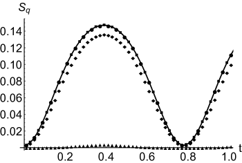
Figure 1: Tsallis entropy ($q=5$) as a function of time for the squeezed vacuum state ($\beta=1/20$) in the parametric amplifier with $\omega_{a}=1$, $\omega_{b}=3$, $\omega=5$, $\kappa=2$, and $\nu=\sqrt{65}/2$. The solid line represents the analytical results, the discrete series denote the numerical results as follows ( circles $n=32$, squares $n=16$, rhombus $n=8$, and triangles $n=4$)

3.2 von Neumann and linear entropies

The von Neumann and linear entropies can also be obtained through the discretization procedure. Making use of the eigenvalues of the partial density matrices, we can write the von Neumann entropy as follows:

$$S_{\rm VN}=-\sum_{i}e^{(1)}_{i}\ln e^{(1)}_{i}=-\sum_{i}e^{(2)}_{i}\ln e^{(2)}_{i}\,.$$ (55)

The linear entropy can also be calculated similarly,

$$S_{L}=1-\sum_{i}e^{(1)2}_{i}=1-\sum_{i}e^{(2)2}_{i}\,.$$ (56)

The evolution of these entropies can be evaluated for the squeezed vacuum state in the parametric amplifier. Using the eigenvalues of the partial density matrix in Eq. (53) it can be shown that the linear entropy is given by

$$S_{L}(t)=\frac{2\left|\eta(t)\right|^{2}}{1+\left|\eta(t)\right|^{2}}\ ,$$ (57)

with $\eta$ given by Eq. (48).

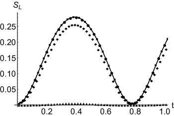
Figure 2: Linear entropy as a function of time for the squeezed vacuum state ($\beta=1/20$) in the parametric amplifier with $\omega_{a}=1$, $\omega_{b}=3$, $\omega=5$, $\kappa=2$, and $\nu=\sqrt{65}/2$. The discrete series denote the same cases as fig. 1

Similarly, for the von Neumann entropy we obtain

$$S_{VN}(t)=-\ln\left(1-\left|\eta(t)\right|^{2}\right)-\frac{\left|\eta(t)\right|^{2}\ln\left(\left|\eta(t)\right|^{2}\right)}{1-\left|\eta(t)\right|^{2}}\ .$$ (58)

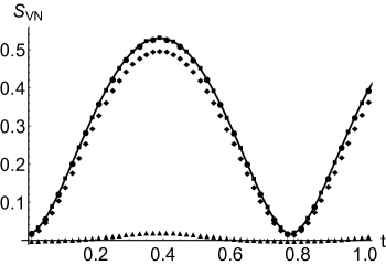
Figure 3: von Neumann entropy as a function of time for the squeezed vacuum state ($\beta=1/20$) in the parametric amplifier with $\omega_{a}=1$, $\omega_{b}=3$, $\omega=5$, $\kappa=2$, and $\nu=\sqrt{65}/2$. The discrete series denote the same cases as fig. 1

The dynamics of the linear and von Neumann entropies are plotted in Figs. 2 and 3, which have the same properties as the Tsallis entropy. They are periodic ($T=\pi/\nu$), and the cut maps with $n=32$ and $n=16$ have a remarkable agreement with the analytic results. The cut map with $n=8$ differs in the vicinity of the maximum values region and the cut map with $n=4$ keeps only some general information on the entropies.

3.3 Logarithmic negativity

The logarithmic negativity criterion is an application of the Peres–Hodorecki criterion [34, 35] to the density matrix. This criterion establishes that the partial transposition of a separable density matrix $\rho=\sum_{i}p_{i}\rho^{(1)}_{i}\otimes\rho^{(2)}_{i}$ satisfies the same properties as the original density matrix, i.e., is hermitian, positively semi-definite and, when there exists entanglement between the modes, the partial transpose of the density matrix exhibits negative eigenvalues. Also the sum of the absolute value of the negative eigenvalues (called negativity) $\sum_{i}|e^{(-)}_{i}|$ grows, if the system is more entangled. The logarithmic negativity reads

$$LN=\log_{2}\left(2\sum_{i}|e^{(-)}_{i}|+1\right)\,,$$ (59)

where the set $\{e^{(-)}_{i}\}$ represents the negative eigenvalues of the partial transpose matrix $\rho^{(1)\rm pt}_{ijkl}~{}=~{}\rho_{kjil}$ or $\rho^{(2)\rm pt}_{ijkl}=\rho_{ilkj}$

The partial transpose of the density matrix for the squeezed vacuum state in the parametric amplifier can be obtained through the expression

$$\rho^{(2)\rm pt}=(1-|\eta(t)|^{2})\sum_{n,m=0}^{\infty}\eta^{n}\eta^{*m}|n,m\rangle\langle m,n|\ ,$$ (60)

which has the following states as eigenvectors:

$$|\Phi_{0}\rangle = |r,r\rangle\ ,$$

$$|\Phi_{\pm}\rangle = \frac{1}{\sqrt{\eta^{r}\eta^{*s}+\eta^{s}\eta^{*r}}}\{\sqrt{\eta^{r}\eta^{*s}}|r,s\rangle\pm\sqrt{\eta^{s}\eta^{*r}}|s,r\rangle\}\ ,$$

with $r\neq s$. These states have eigenvalues

$$(1-|\eta|^{2})|\eta|^{2r},\ \pm(1-|\eta|^{2})|\eta|^{r+s}\ ,$$

respectively. Thus, the negativity reads

$$\frac{|\eta|}{1-|\eta|}\,,$$

and the logarithmic negativity is

$${\rm LN}=\log_{2}\left(\frac{1+|\eta|}{1-|\eta|}\right)\,.$$ (61)

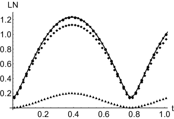
Figure 4: Logarithmic negativity as a function of time for the squeezed vacuum state ($\beta=1/20$) in the parametric amplifier with $\omega_{a}=1$, $\omega_{b}=3$, $\omega=5$, $\kappa=2$, and $\nu=\sqrt{65}/2$.The solid line represents the analytical results, the discrete series denote the numerical results for a partition of $n$ elements as follows ( circles $n=1024$, squares $n=512$, rhombus $n=256$, and triangles $n=128$)

In Fig. 4, we show the logarithmic negativity as a function of time. To calculate these quantities, we use a cut map of the bipartite partial transpose density matrix with $n=1024,512,256,128$. Note that these values are two orders of magnitude larger, and thus the procedure is computationally more complex. The differences between the analytic and numerical results are negligible for the cut maps with $n=1024$ and $n=512$. For the cut map with $n=256$, one finds larger discrepancies than the previous maps around the maxima of the analytic curve. For the cut map with $n=128$, some information on the logarithmic negativity is preserved, as it happens for the other entanglement calculations.

4 Other observables

The study of other observables obtained through the established nonlinear map can be carried out similarly. As an example, we consider the covariance matrix $\boldsymbol{\sigma}(t)$, which for the parametric amplifier is defined by

$$\boldsymbol{\sigma}(t) = \left(\begin{array}[]{cccc}\sigma_{p_{1}p_{1}}&\sigma_{p_{1}p_{2}}&\sigma_{p_{1}q_{1}}&\sigma_{p_{1}q_{2}}\\ \sigma_{p_{2}p_{1}}&\sigma_{p_{2}p_{2}}&\sigma_{p_{2}q_{1}}&\sigma_{p_{2}q_{2}}\\ \sigma_{q_{1}p_{1}}&\sigma_{q_{1}p_{2}}&\sigma_{q_{1}q_{1}}&\sigma_{q_{1}q_{2}}\\ \sigma_{q_{2}p_{1}}&\sigma_{q_{2}p_{2}}&\sigma_{q_{2}q_{1}}&\sigma_{q_{2}q_{2}}\end{array}\right)\,,$$ (66)

with $\sigma_{xy}=\frac{1}{2}\langle\{x,y\}\rangle-\langle x\rangle\langle y\rangle$. Using the discretized form of the density matrix, we calculate different covariances as follows:

$$\sigma_{p_{1}p_{2}} = -\sum_{i=1}^{n-1}\sum_{j=1}^{n-1}\rho_{i+1,j+1,i+1,j+1}+\sum_{i=1}^{n-1}\sum_{j=1}^{n}\rho_{i+1,j,i+1,j}+\sum_{i=1}^{n}\sum_{j=1}^{n-1}\rho_{i,j+1,i,j+1}$$ (67)

$$- \sum_{i=1}^{n}\sum_{j=1}^{n}\rho_{i,j,i,j}\,,$$

$$\sigma_{p_{k}p_{k}} = -\sum_{i=1}^{n-1}\rho^{(k)}_{i,i+1}+2\sum_{i=2}^{n}\rho^{(k)}_{i,i-1}-\sum_{i=1}^{n}\rho^{(k)}_{i,i}\,,$$ (68)

with $k=1,2$,

$$\sigma_{q_{k}q_{k}} = \sum_{i=1}^{n}\rho^{(k)}_{i,i}z^{2}(\Delta z)^{2}-\left(\sum_{i=1}^{n}\rho^{(k)}_{i,i}z(\Delta z)^{2}\right)^{2}\,,$$ (69)

where for the first mode $z=x$, while for the second one $z=y$. Also

$$\sigma_{q_{k}p_{k}} = -\frac{i}{2}\Bigl{(}\sum_{i=1}^{n-1}\rho^{(k)}_{i+1,i}z-2\sum_{i=1}^{n}\rho^{(k)}_{i,i}z+\sum_{i=1}^{n-1}\rho^{(k)}_{i+1,i}z\Bigr{)}\Delta z\,.$$ (70)

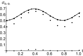
Figure 5: The covariance $\sigma_{q_{1}q_{1}}$ as a function of time for the squeezed vacuum state ($\beta=1/20$) in the parametric amplifier with $\omega_{a}=1$, $\omega_{b}=3$, $\omega=5$, $\kappa=2$, and $\nu=\sqrt{65}/2$. The discrete series denote the same cases as fig. 1

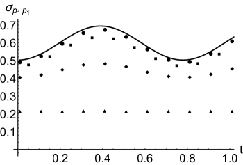
Figure 6: The covariance $\sigma_{p_{1}p_{1}}$ as a function of time for the squeezed vacuum state ($\beta=1/20$) in the parametric amplifier with $\omega_{a}=1$, $\omega_{b}=3$, $\omega=5$, $\kappa=2$, and $\nu=\sqrt{65}/2$. The discrete series denote the same cases as fig. 1

The covariance matrix elements $\sigma_{q_{1}q_{1}}$ and $\sigma_{p_{1}p_{1}}$ as functions of time are exhibited in Figs. 5 and 6; we see that the cut maps, showing good agreement with the analytic results for the entanglement, also display a good agreement in the covariances matrix elements. In the case of $\sigma_{p_{1}p_{1}}$, the numerical results are worse than the results for $\sigma_{q_{1}q_{1}}$, because for the quadrature $p$ it is necessary to approximate the first derivative (and also the second derivative) of the density matrix by the expression $\langle x,y|p\rho|x^{\prime},y^{\prime}\rangle\simeq-i(\rho(x,y+\Delta y;x^{\prime},y^{\prime})-\rho(x,y;x^{\prime},y^{\prime}))/\Delta y$. This approximation has an associated error of $(\Delta y)^{2}$, which can be noticed in Fig. 6.

5 Conclusions

In this work, we proposed the discretization of the density matrices of continuous variables as nonlinear positive maps. The resulting discrete density matrix can be used to calculate the quantum properties of the system, such as entanglement between the modes. Specifically, the two-mode entanglement measures used in this work are the Tsallis, von Neumann and linear entropies and the logarithmic negativity. This procedure is demonstrated using the two-mode squeezed vacuum state evolving in the parametric amplifier. The squeezed vacuum state presents a periodic entanglement with period $T=\pi/\nu$.

The entanglement measures based on Tsallis entropy, von Neumann entropy and linear entropy are obtained using the discretization procedure for the reduced density matrix with different dimensions $n=32,16,8,4$. The numerical values of entropies for the procedure using discretization with $n=32$ and $n=16$ are almost equal to the analytic expressions of those quantities; in the case of $n=8$, the error between the numerical and analytic results is larger than in the previous case. In the case of $n=4$, the results are completely different, although the periodic behavior remains. The logarithmic negativity, being a two-mode measure of the entanglement, was obtained using a larger dimension than with the entropies, which can be obtained using only one mode. In this case, the two-mode density matrix was discretized using the different dimensions $n=1024,512,256,128$; the analytic and numerical results are compared giving a very good agreement for $n=1024$ and $n=512$; in the case of $n=256$, the results are not always equal; and in the case of $n=128$, the results are completely different although, as in the case of entropies, the periodic behavior is still present.

We presented the nonlinear positive maps (called cut maps) of the density $N$$\times$$N$ matrix onto the density $n$$\times$$n$ matrix, with $n<N$. We demonstrated an example of the cut map for the case of qutrit density matrix. The structure of the map is obtained following the procedure of mapping the density matrix of continuous variables onto a finite-dimensional matrix. It is worth pointing out that the cut positive maps and the discretization positive maps provide the density matrices of smaller dimensions, but these matrices almost preserve information on quantum correlations available in the initial matrices. Further applications of the map will be considered in a future paper.

References

- [1] E. Schrödinger, Ann Phys., 79, 361; 81, 109 (1926).
- [2] L.D. Landau, The damping problem in wave mechanics. Z. Phys., 45 430-441 (1927).
- [3] J. Von Neumann, Wahrscheinlichkeitstheoretischer Aufbau der Quantenmechanik. Nach. Ges. Wiss. Göttingen, 11 245-272 (1927).
- [4] J. Von Neumann, Mathematische Grundlagen der Quantummechanik, Springer, Berlin (1932).
- [5] M. D. Choi, Completely Positive Linear Maps on Complex Matrices, Linear Algebra and its Applications, 10 285-290 (1975).
- [6] W. F. Stinespring, Positive Functions on C*-algebras, Proceedings of the American Mathematical Society, 211-216, 1955
- [7] E. C. G. Sudarshan, P. M. Mathews and J. Rau, Phys. Rev. 121 920 (1961).
- [8] V. I. Man’ko and R. S. Puzko, Europhys. Lett., 109, 50005 (2015).
- [9] V. I. Man’ko, G. Marmo, A. Simoni and F. Ventriglia, Phys. Lett. A, 372 6490 (2008).
- [10] P. Hausladen, R. Jozsa, B. Schumacher, M. Westmoreland, Phys. Rev. A, 54 1869 (1996).
- [11] S. Lloyd, Phys. Rev. A, 55 1613 (1997).
- [12] C. H. Bennett, P. W. Shor, J. A. Smolin, and A. V. Thapliyal, Phys. Rev. Lett., 83 3081 (1999).
- [13] C. H. Bennett, P. W. Shor, J. A. Smolin, and A. V. Thapliyal, IEEE Trans. Inform. Theor., 48 2637 (2002).
- [14] M.A. Man’ko and V. I. Man’ko, J. Russ. Laser Res., 34 203 (2013).
- [15] V. N. Chernega and O. V. Man’ko, J. Russ. Laser Res., 34 383 (2013).
- [16] M.A. Man’ko and V. I. Man’ko, Phys. Scr., T160 014030 (2014).
- [17] V. N. Chernega and O. V. Man’ko, J. Russ. Laser Res., 35 27 (2014).
- [18] M. A. Man’ko and V. I. Man’ko, Entropy, 17 2876 (2015).
- [19] V. I. Man’ko and L.V. Markovich, J. Russ. Laser Res., 36 110 (2015).
- [20] K. Kraus, States, Effects, and Operations: Fundamental Notions of Quantum Theory, Springer, Berlin, 1983
- [21] V. Gorini, A. Kossakowski, E. C. G. Sudarshan, Completely positive dynamical semigroups of N-level systems, J. Math. Phys., 17 82182 (1976) .
- [22] G. Lindblad, On the generators of quantum dynamical semigroups, Commun. Math. Phys., 48 119130 (1976).
- [23] E. Andersson, J. D. Cresser and M. J. W. Hall, J. Mod. Opt., 54 1695 (2007)
- [24] V.I. Man’ko, G. Marmo, E.C.G. Sudarshan and F. Zaccaria Symmetries in Science XI, Kluwer Academic Publishers, Dordrecht 395 (2004).
- [25] Yu. M. Belousov, S. N. Filippov, V. I. Man’ko, and I. V. Traskunov, J. Russ. Laser Res., 32 584 (2011).
- [26] D. Chruscinski, V. I. Man’ko, G. Marmo, and F. Ventriglia, Phys. Scr., 87 045015 (2013).
- [27] J. A. López-Saldívar, A. Figueroa, O. Castaños, R. López-Peña, M.A. Man’ko, and V. I. Man’ko, J. Russ. Laser Res., 37 23 (2016).
- [28] H. Umegaki, Kodai Math. Sem Rep., 14 59 (1962).
- [29] G. S. Agarwal, Phys. Rev. A, 3 828 (1971).
- [30] A. Serafini, F. Illuminati and S. De-Siena, J. Phys. B: At. Mol. Opt. Phys., 37 L21 (2004).
- [31] A. V. Dodonov, V. V. Dodonov and S. S. Mizrahi, J. Phys. A: Math. Gen., 38 683 (2005).
- [32] C. Tsallis, Nonextensive statistical mechanics and thermodynamics: historical background and present status, in: S. Abe and Y. Okamoto (Eds.), Nonextensive Statistical Mechanics and Its Applications, Lecture Notes in Physics, Springer, Berlin, 560 3 (2001).
- [33] J. von Neumann, Mathematical Foundations of Quantum Mechanics, Princeton University Press (1955).
- [34] Asher Peres, Separability Criterion for Density Matrices, Phys. Rev. Lett., 77 1413-1415 (1996)
- [35] M. Horodecki, P. Horodecki, R. Horodecki, Separability of Mixed States: Necessary and Sufficient Conditions, Phys. Lett. A, 223 1-8 (1996).
- [36] C. E. Shannon, A Mathematical Theory of Communication’ Bell Syst. Tech. J., 27 379-423 (1948).
- [37] A. Rényi, Probability Theory, North-Holland, Amsterdam (1970).