Black hole nonmodal linear stability: odd perturbations of Reissner-Nordström

Abstract

Following a program on black hole nonmodal linear stability initiated in Phys. Rev. Lett.  112 (2014) 191101, we study odd linear perturbations of the Einstein-Maxwell equations around a Reissner-Nordström (A)dS black hole. We show that all the gauge invariant information in the metric and Maxwell field perturbations is encoded in the spacetime scalars $\mathcal{F}=\delta(F^{*}_{\alpha\beta}F^{\alpha\beta})$ and $\mathcal{Q}=\delta(\tfrac{1}{48}C^{*}_{\alpha\beta\gamma\delta}C^{\alpha\beta\gamma\delta})$, where $C_{\alpha\beta\gamma\delta}$ is the Weyl tensor, $F_{\alpha\beta}$ the Maxwell field, a star denotes Hodge dual and $\delta$ means first order variation, and that the linearized Einstein-Maxwell equations are equivalent to a coupled system of wave equations for $\mathcal{F}$ and $\mathcal{Q}$. For nonnegative cosmological constant we prove that $\mathcal{F}$ and $\mathcal{Q}$ are pointwise bounded on the outer static region. The fields are shown to diverge as the Cauchy horizon is approached from the inner dynamical region, providing evidence supporting strong cosmic censorship. In the asymptotically AdS case the dynamics depends on the boundary condition at the conformal timelike boundary and there are instabilities if Robin boundary conditions are chosen.

I Introduction

General Relativity coupled to Maxwell fields admits static charged black hole solutions in spacetime dimensions $d=4$ and higher. The spacetimes are warped products ${\cal M}={\cal N}\times_{r^{2}}\sigma^{n}$ of a two dimensional Lorentzian “orbit manifold” ${\cal N}$ with line element $\tilde{g}_{ab}(y)dy^{a}dy^{b}$ and an $n=d-2$ dimensional Riemannian “horizon manifold” $\sigma^{n}$ with metric $\hat{g}_{AB}(x)\,dx^{A}dx^{B}$ (see, e.g., Kodama:2003kk ):

$$g_{\alpha\beta}dz^{\alpha}dz^{\beta}=\tilde{g}_{ab}(y)\,dy^{a}dy^{b}+r^{2}(y)\hat{g}_{AB}(x)\,dx^{A}dx^{B}.$$ (1)

In four dimensions, the solution with $S^{2}$ horizon is the Reissner-Nordström black hole. If we use the standard angular coordinates $\hat{g}_{ij}(x)\,dx^{i}dx^{j}=d\theta^{2}+\sin^{2}\theta\;d\phi^{2}$ and static coordinates $(t,r)$ for the orbit manifold, the Reissner-Nordström metric is given by

$$g_{\alpha\beta}dz^{\alpha}dz^{\beta}=-fdt^{2}+\frac{dr^{2}}{f}+r^{2}(d\theta^{2}+\sin^{2}\theta\;d\phi^{2}),$$ (2)

where the norm $f$ of the Killing vector $k^{a}=\partial/\partial t$ in (2) is

$$f=1-\frac{2M}{r}+\frac{Q^{2}}{r^{2}}-\frac{\Lambda}{3}r^{2}.$$ (3)

In (3), $\Lambda$ is the cosmological constant, and $M$ and $Q$ are constants of integration that correspond to mass and charge respectively. The metric (2) together with the Maxwell field

$$F=\frac{Q}{r^{2}}\;dt\wedge dr,$$ (4)

solves the Einstein-Maxwell field equations

$$G_{\alpha\beta}+\Lambda g_{\alpha\beta}=8\pi T_{\alpha\beta},$$ (5)

$$\nabla_{[\alpha}F_{\beta\gamma]}=0,$$ (6)

$$\nabla^{\beta}F_{\alpha\beta}=0,$$ (7)

where

$$T_{\alpha\beta}=\tfrac{1}{4\pi}\left(F_{\alpha\gamma}F_{\beta}{}^{\gamma}-\tfrac{1}{4}g_{\alpha\beta}F_{\gamma\delta}F^{\gamma\delta}\right).$$ (8)

Note that, since $T_{\alpha\beta}$ is traceless, (5) is equivalent to

$$R_{\alpha\beta}-\Lambda g_{\alpha\beta}=8\pi T_{\alpha\beta}$$ (9)

We assume $Q\neq 0$ and focus in the black hole cases, which are those for which there is an outer static ($f>0$) region, that is, either $\Lambda\leq 0$ and $0<r_{h}<r<\infty$, or $\Lambda>0$ and $0<r_{h}<r<r_{c}$. Here the event and cosmological horizons $r=r_{h}$ and $r=r_{c}$ are simple zeros of the quartic polynomial $r^{2}f$ if the black hole is non extremal. The range of values of $M,Q$ and $\Lambda$ giving black holes can be found in Appendix A of Kodama:2003kk .

We are interested in proving the non-modal linear stability of the outer static region of the solution (2)-(4) of the field equations (5)-(8). By this we mean Dotti:2013uxa Dotti:2016cqy , showing that:

1. there are gauge invariant (both in the Maxwell and linear gravity sense) scalar fields $\chi:{\cal M}\to\mathbb{R}$ that contain the same information as the perturbation $\mathcal{F}_{\alpha\beta}=\delta F_{\alpha\beta}$ of the electromagnetic field and the gauge class $[h_{\alpha\beta}]$ of the metric perturbation $h_{\alpha\beta}=\delta g_{\alpha\beta}$, and measure the distortion of the geometry and the Maxwell field. By “contain the same information” we mean that $h_{\alpha\beta}$ in a given gauge and $\mathcal{F}_{\alpha\beta}$ can be obtained by applying some injective linear functional on the fields $\chi$.

2. the fields $\chi$ are pointwise bounded on the outer static region by constants that depends on the initial data of the perturbation on a Cauchy surface.

The perturbed metric and Maxwell fields can be expanded in series involving rank 0,1, and 2 eigentensor fields of the horizon manifold Laplace-Beltrami (LB) operator, with “coefficients” that are tensor fields in the orbit space $\mathcal{N}$; this is the mode expansion of $h_{\alpha\beta}$ and $\mathcal{F}_{\alpha\beta}$ Kodama:2003kk . The linearized Einstein-Maxwell equations (LEME) do not mix modes. A master scalar field $\mathcal{N}\to\mathbb{R}$ can be extracted for each mode such that the LEME reduce to an infinite set of scalar wave equations on $\mathcal{N}$, one for each master scalar field. This was proved in four dimensional General Relativity in the seminal black hole stability papers Regge:1957td Zerilli:1970se Zerilli:1974ai and in higher dimensions more recently by Kodama and Ishibashi (see, eg.g. Kodama:2003kk and Ishibashi:2011ws ). Prior notions of linear stability are based on the boundedness of the master fields on the orbit manifold $\mathcal{N}$, we call this modal (linear) stability. In the case of four dimensional asymptotically flat charged black holes the modal linear stability was proved by Zerilli and Moncrief in the series of articles Zerilli:1974ai ; Moncrief:1974gw ; Moncrief:1974ng ; Moncrief:1975sb (see also wald )

The limitations of the modal linear stability notion are explained in Dotti:2013uxa and Dotti:2016cqy , where a non modal stability concept based on i) and ii) above was proved to hold for the Schwarzschild and Schwarzschild de Sitter black holes. In these papers the fields $\chi$ in i) are gauge invariant combinations of perturbations of scalars made out of contractions of the Weyl tensor, its dual, and its first covariant derivative.

For Einstein-Maxwell black holes the extra degrees of freedom coming from the Maxwell field have to be accounted for. Perturbations naturally split into two decoupled types: odd and even (Section II). In this paper we prove the non modal linear stability of the Reissner-Nordström black hole under odd perturbations. The fields $\chi$ that fulfill the requirements i) and ii) above are the first order perturbation of the scalars obtained by contracting the Maxwell and Weyl tensors with their Hodge duals: $\mathcal{F}=\delta(F^{*}_{\alpha\beta}F^{\alpha\beta})$ and $\mathcal{Q}=\delta(\tfrac{1}{48}C^{*}_{\alpha\beta\gamma\delta}C^{\alpha\beta\gamma\delta})$. These fields are shown to satisfy a coupled system of wave equations in the Reissner-Nordström background, and this fact is used to prove their pointwise boundedness on the outer static region. We defer to future work the treatment of even perturbations.

II Linearized Einstein-Maxwell equations

Let $(g({\varepsilon})_{\alpha\beta},F(\varepsilon)_{\alpha\beta})$ be a one-parameter family of solutions of the Einstein-Maxwell equations (8)-(9), with $g({\varepsilon=0})_{\alpha\beta}$ and $F(\varepsilon=0)_{\alpha\beta}$ the Reissner-Nordström fields (2)-(4). Note that all fields in this paper are assumed to be jointly smooth in the spacetime coordinates and (in the case of one-parameter families) the perturbation parameter. The perturbation fields

$$h_{\alpha\beta}\equiv\frac{d}{d\varepsilon}\bigg{|}_{\varepsilon=0}g({\varepsilon})_{\alpha\beta},\;\;\;\mathcal{F}_{\alpha\beta}\equiv\frac{d}{d\varepsilon}\bigg{|}_{\varepsilon=0}F({\varepsilon})_{\alpha\beta}$$ (10)

satisfy the linearized Einstein-Maxwell equations (LEME):

$$\frac{d}{d\varepsilon}\bigg{|}_{\varepsilon=0}G_{\alpha\beta}(g(\varepsilon))+\Lambda h_{\alpha\beta}=2\frac{d}{d\varepsilon}\bigg{|}_{\varepsilon=0}\left[F({\varepsilon})_{\alpha\gamma}F({\varepsilon})_{\beta\mu}g(\varepsilon)^{\gamma\mu}-\tfrac{1}{4}g({\varepsilon})_{\alpha\beta}\left(F({\varepsilon})_{\mu\nu}F({\varepsilon})_{\mu^{\prime}\nu^{\prime}}g(\varepsilon)^{\mu\mu^{\prime}}g(\varepsilon)^{\nu\nu^{\prime}}\right)\right],$$ (11)

$$\frac{d}{d\varepsilon}\bigg{|}_{\varepsilon=0}\partial_{[\alpha}F({\varepsilon})_{\beta\gamma]}=0,$$ (12)

$$\frac{d}{d\varepsilon}\bigg{|}_{\varepsilon=0}\nabla_{\beta}F({\varepsilon})^{\alpha\beta}=0.$$ (13)

As in equation (1), we adopt the notation in Chaverra:2012bh and use lower case indexes $a,b,c,d,e$ for tensors on the orbit manifold ${\cal N}$, upper case indexes $A,B,C,D,...$ for tensors on $S^{2}$, and Greek indexes for space-time tensors, and follow the additional convention in Dotti:2016cqy that

$$\alpha=(a,A),\beta=(b,B),\gamma=(c,C),\delta=(d,D),...\text{ etc. }$$ (14)

Tensor fields introduced with a lower $S^{2}$ index (say $Z_{A}$) and then shown with an upper $S^{2}$ index are assumed to have been acted on with the unit $S^{2}$ metric inverse $\hat{g}^{AB}$, (i.e., in our example, $Z^{A}\equiv\hat{g}^{AB}Z_{B}$), and similarly with upper $S^{2}$ indexes moving down. This has to be kept in mind to avoid wrong $r^{\pm 2}$ factors in the equations. $\widetilde{D}_{a},\tilde{\epsilon}_{ab}$ and $\tilde{g}^{ab}$ are the covariant derivative, volume form (any chosen orientation) and metric inverse for the $\mathcal{N}$ orbit space; $\widehat{D}_{A}$ and $\hat{\epsilon}_{AB}$ are the covariant derivative and volume form $\sin(\theta)d\theta\wedge d\phi$ on the unit sphere. As an example, the Laplacian on scalar fields can be written in terms of the differential operators $\widetilde{D}_{a}$ and $\widehat{D}_{A}$ as

$$\nabla_{\alpha}\nabla^{\alpha}\Phi=\widetilde{D}_{a}\widetilde{D}^{a}\Phi+\frac{2}{r}(\widetilde{D}^{b}r)(\widetilde{D}_{b}\Phi)+\frac{1}{r^{2}}\widehat{D}_{A}\widehat{D}^{A}\Phi.$$ (15)

The linearized field equations, (10) and (12) imply that locally there exists a vector potential $A_{\alpha}$ such that

$$\mathcal{F}_{\alpha\beta}=\partial_{\alpha}A_{\beta}-\partial_{\beta}A_{\alpha},$$ (16)

The linear fields entering the LEME are $h_{\alpha\beta}$ and $A_{\alpha}$. Under the index convention (14) the covector field $A_{\alpha}$ is written

$$A_{\alpha}=(A_{a},A_{A}).$$ (17)

From the $S^{2}$ viewpoint $A_{\alpha}$ contains two scalar fields $A_{a}^{+}\equiv A_{a}$ and a covector field $A_{A}$. Using Proposition 2.1 in Ishibashi:2004wx and the fact that the first Betti number of $S^{2}$ is zero (which implies that divergence free $S^{2}$ covectors are of the form $\hat{\epsilon}_{A}{}^{B}\widehat{D}_{B}P$, with $P$ an $S^{2}$ scalar field), we can write $A_{A}=\widehat{D}_{A}A^{+}+\hat{\epsilon}_{A}{}^{C}\widehat{D}_{C}A^{-}$, thus

$$A_{\alpha}=(A^{+}_{a},\widehat{D}_{A}A^{+}+\hat{\epsilon}_{A}{}^{C}\widehat{D}_{C}A^{-}).$$ (18)

The scalar fields $A^{\pm}$ are unique if they are required to belong to $L^{2}(S^{2})_{>0}$ Dotti:2016cqy , where $L^{2}(S^{2})_{>\ell_{o}}$ is the space of square integrable functions on $S^{2}$ orthogonal to the $\ell=0,1,...,\ell_{o}$ eigenspaces of the LB operator, and $\ell$ labels the LB scalar field eigenvalue $-\ell(\ell+1)$. The plus (even) and minus (odd) signs on tensor fields refer to the way they transform when pull backed by the antipodal map $P$ on $S^{2}$ Dotti:2013uxa .
A symmetric tensor field $S_{\alpha\beta}=S_{\beta\alpha}$,

$$S_{\alpha\beta}=\left(\begin{array}[]{cc}S_{ab}&S_{aB}\\ S_{Ab}&S_{AB}\end{array}\right),$$ (19)

such as the perturbations of the metric, the Einstein and the energy momentum tensor fields, contains three $S^{2}$ scalar fields $S_{ab}^{+}\equiv S_{ab}$, two $S^{2}$ covector fields $S_{aB}$ and a symmetric tensor field $S_{AB}$. The $S^{2}$ covectors can be decomposed as in (18)

$$S_{aB}=\widehat{D}_{B}S_{a}^{+}+\hat{\epsilon}_{B}{}^{C}\widehat{D}_{C}S_{a}^{-},$$ (20)

where again $S_{a}^{\pm}$ are unique if their components are in $L^{2}(S^{2})_{>0}$. From Proposition 2.2 in Ishibashi:2004wx and the fact that there are no transverse traceless symmetric rank two tensor fields on $S^{2}$, follows that

$$S_{AB}=\widehat{D}_{(A}(\epsilon_{B)C}\widehat{D}^{C}S^{-})+\left(\widehat{D}_{A}\widehat{D}_{B}-\tfrac{1}{2}\hat{g}_{AB}\widehat{D}^{C}\widehat{D}_{C}\right)S^{+}+\tfrac{1}{2}\;S_{T}^{+}\;\hat{g}_{AB},\;\;(S_{T}^{+}=S_{C}{}^{C}).$$ (21)

The fields $S^{\pm}$ are unique if required to belong to $L^{2}(S^{2})_{>1}$ Dotti:2016cqy . In this way, the symmetric field $S_{\alpha\beta}$ is replaced by two sets of fields, even (+) and odd (-):

$$S_{\alpha\beta}\sim\{S_{ab}^{+}=S_{ab},\;S_{a}^{+},\;S^{+},\;S_{T}^{+}\}\cup\{S_{a}^{-},\;S^{-}\}.$$ (22)

If we decompose the linearized symmetric tensor fields $h_{\alpha\beta}$, $dG_{\alpha\beta}/d\varepsilon|_{0}\equiv\mathcal{G}_{\alpha\beta}$ and $dT_{\alpha\beta}/d\varepsilon|_{0}\equiv\mathcal{T}_{\alpha\beta}$ as in (19)-(22), we get the following sets of even and odd fields:

$${h}_{\alpha\beta} \sim\{h_{ab}^{+},\;h_{a}^{+},\;h^{+},\;{h}_{T}^{+}\}\cup\{h_{a}^{-},\;h^{-}\}$$ (23)

$$\mathcal{G}_{\alpha\beta} \sim\{G_{ab}^{+},\;G_{a}^{+},\;G^{+},\;G_{T}^{+}\}\cup\{G_{a}^{-},\;G^{-}\}$$ (24)

$$\mathcal{T}_{\alpha\beta} \sim\{T_{ab}^{+},\;T_{a}^{+},\;T^{+},\;T_{T}^{+}\}\cup\{T_{a}^{-},\;T^{-}\}.$$ (25)

Group theoretical arguments (refer to Section 2 of Ishibashi:2004wx ) indicate that the LEME involving the even fields in (18) (23)-(25) decouple from those involving the odd fields, so we can switch off one sector and study purely odd or even perturbations. Odd perturbations are the subject of this paper.

We will find it useful to introduce the square angular momentum operator

$$\mathbf{J}^{2}\equiv(\pounds_{J_{(1)}})^{2}+(\pounds_{J_{(2)}})^{2}+(\pounds_{J_{(3)}})^{2},$$ (26)

where $J_{(1)},J_{(2)}$ and $J_{(3)}$ are $S^{2}$ (and thus spacetime) Killing vector fields corresponding to rotations around orthogonal axis in $\mathbb{R}^{3}\supset S^{2}$, with maximum orbit orbit lengths set to $2\pi$ (e.g., $J_{(3)}=\partial/\partial_{\phi}$). On $S^{2}$ scalar fields the operator $\mathbf{J}^{2}$ agrees with the $S^{2}$ LB operator $\widehat{D}^{A}\widehat{D}_{A}$, but these two operators act differently on higher rank tensors. A key property of $\mathbf{J}^{2}$ is that it commutes with $\nabla_{\alpha}$, $\widetilde{D}_{a}$ and $\widehat{D}_{A}$, this follows from $[\nabla_{a},\pounds_{J_{k}}]=0=[\widehat{D}_{A},\pounds_{J_{k}}]=[\widetilde{D}_{a},\pounds_{J_{k}}]$. The modal decomposition consists in expanding the $S^{2}$ scalars in (18) (23)-(25) in a real basis of spherical harmonics of $S^{2}$, which are eigenfields of $\mathbf{J}^{2}$ with eigenvalues $-\ell(\ell+1)$, the eigenspaces being of of dimension $2\ell+1$. The differential operators that give a symmetric tensor $S_{\alpha\beta}$ or a covector $A_{\alpha}$ in terms of these $S^{2}$ scalars commute with $\mathbf{J}^{2}$. Thus, if the $S^{2}$ scalar fields in (23) and (18) lie on the $\ell$ eigenspace, then $h_{\alpha\beta},\mathcal{G}_{\alpha\beta},\mathcal{F}_{\alpha\beta}$ will all be eigentensors of $\mathbf{J}^{2}$ with eigenvalue $-\ell(\ell+1)$, i.e., different modes stay unmixed. The distinction between even and odd modes can now be stated in a precise way: if $X^{\pm}$ is a covector (18) or symmetric field $S_{\alpha\beta}$ (19)-(22) of a given parity, made out of scalars of harmonic numbers ($\ell,m)$, then $\mathbf{J}^{2}X^{\pm}=-\ell(\ell+1)X^{\pm}$ and $P_{*}X^{\pm}=\pm(-1)^{\ell}X^{\pm}$.

We will assume that $A^{\pm},S_{a}^{\pm}$ to $L^{2}(S^{2})_{>0}$ and $S^{\pm}$ to $L^{2}(S^{2})_{>1}$, since then the linear operators $(A^{+},A^{-})\to A_{\alpha}$ in (18), and $\{S_{ab}^{+},\;S_{a}^{+},\;S^{+},s^{+}\}\cup\{S_{a}^{-},\;S^{-}\}\to S_{\alpha\beta}$ in (21) are injective Dotti:2016cqy . Consequently, the odd sector LEME (11) are equivalent to

$$G^{-}_{a}+\Lambda h^{-}_{a}=8\pi T_{a}^{-},$$ (27)

$$G^{-}+\Lambda h^{-}=8\pi T^{-}.$$ (28)

II.1 Odd sector perturbations

Odd perturbations are those for which the plus fields in (18) and (23) are zero, that is

$$h_{\alpha\beta}=\left(\begin{array}[]{cc}0&\hat{\epsilon}_{B}{}^{C}\widehat{D}_{C}h_{a}^{-}\\ \hat{\epsilon}_{A}{}^{C}\widehat{D}_{C}h_{b}^{-}&\widehat{D}_{(A}(\epsilon_{B)C}\widehat{D}^{C}h^{-})\end{array}\right),\;\;\;\;\;\;\mathcal{F}_{\alpha\beta}=\left(\begin{array}[]{cc}0&\widetilde{D}_{a}(\hat{\epsilon}_{B}{}^{C}\widehat{D}_{C}A^{-})\\ -\widetilde{D}_{b}(\hat{\epsilon}_{A}{}^{C}\widehat{D}_{C}A^{-})&-\epsilon_{AB}\widehat{D}^{C}\widehat{D}_{C}A^{-}\end{array}\right),$$ (29)

with $A^{-},h_{a}^{-}\in L^{2}(S^{2})_{>0}$ and $h^{-}\in L^{2}(S^{2})_{>1}$, which are conditions that guarantee their uniqueness, as explained at the end of the previous Section. $U(1)$ gauge transformations of the Maxwell field are of the form $A_{\alpha}\to A_{\alpha}+\partial_{\alpha}B$ and therefore affect only the even piece of the vector potential (18) leaving $A^{-}$ invariant.
Under a coordinate gauge transformation (infinitesimal diffeomorphism) along the odd vector field $\zeta^{\alpha}=(0,\hat{\epsilon}^{AB}\widehat{D}_{B}\xi)$, $\xi\in L^{2}(S^{2})_{>0}$, $h_{\alpha\beta}$ and $\mathcal{F}_{\alpha\beta}$ transform into the physically equivalent fields:

$$h^{\prime}_{\alpha\beta}=h_{\alpha\beta}+\pounds_{\zeta}g_{\alpha\beta},\;\;\mathcal{F}^{\prime}_{\alpha\beta}=\mathcal{F}_{\alpha\beta}+\pounds_{\zeta}F_{\alpha\beta}=\mathcal{F}_{\alpha\beta}.$$ (30)

We call $\mathcal{L}_{-}$ the set of odd solutions $(h_{\alpha\beta},\mathcal{F}_{\alpha\beta})$ of the LEME (11)-(13) mod the equivalence relation $h_{\alpha\beta}\sim h^{\prime}_{\alpha\beta}$ above, that is, if $[h_{\alpha\beta}]$ denotes equivalence class under the first transformation (30), then

$$\mathcal{L}_{-}=\{([h_{\alpha\beta}],\mathcal{F}_{\alpha\beta})\;|\;(h_{\alpha\beta},\mathcal{F}_{\alpha\beta})\;\text{ is an odd solution of (\ref{1})-(\ref{3}) }\}.$$ (31)

The transformation (30) is equivalent to

$$h_{a}^{-}\to h_{a}^{-}+r^{2}\widetilde{D}_{a}\xi,\;\;\;h^{-}\to h^{-}+r^{2}\xi_{>1},\;\;\;A^{-}\to A^{-},$$ (32)

and implies that the field $A\equiv A^{-}$ is gauge invariant. If we project $h_{a}^{-}=(h_{a}^{-})^{(\ell=1)}+(h_{a}^{-})^{(>1)}$ onto its $L^{2}(S^{2})_{(\ell=1)}$ and $L^{2}(S^{2})_{>1}$ pieces, and similarly for the other fields, and keep in mind that $h^{-}=(h^{-})^{(>1)}$, we find that:

1. The $\mathcal{N}$ 1-form $h_{a}^{>1}\in L^{2}(S^{2})_{>1}$ defined by

   $$h_{a}^{>1}\equiv(h_{a}^{-})^{>1}-r^{2}\widetilde{D}_{a}(r^{-2}h^{-})$$ (33)

   is gauge invariant.

2. There exists a gauge for $(h_{\alpha\beta})^{>1}$ such that $h^{-}=0$. In view of (33), in this gauge

   $$(h_{\alpha\beta})^{>1}=\left(\begin{array}[]{cc}0&\hat{\epsilon}_{B}{}^{C}\widehat{D}_{C}h_{a}^{>1}\\ \hat{\epsilon}_{A}{}^{C}\widehat{D}_{C}h_{b}^{>1}&0\end{array}\right)$$ (34)

   This is the well known Regge-Wheeler (RW) gauge for $(h_{\alpha\beta})^{>1}$, and is unique, in the sense that, according to (32), applying to (34) any gauge transformation that is non trivial in the $\ell>1$ sector, spoils the $h^{-}=0$ condition.

3. For $\ell=1$ the only possible gauge invariant metric field is Sarbach:2001qq

   $$\mathcal{Z}:=\tilde{\epsilon}^{cd}\widetilde{D}_{c}\left(\frac{h_{d}^{(\ell=1)}}{r^{2}}\right)$$ (35)

From now on we work in RW gauge (34), then we set $h^{-}=0$ in (29) and replace $h_{a}^{-}$ with $h_{a}=(h_{a})^{(\ell=1)}+h_{a}^{>1}$. With this choice the absolute value $g$ of the determinant of the metric agrees (to linear order) with the absolute value $g_{o}$ of the unperturbed metric determinant, then

$$\sqrt{g}=\sqrt{g_{o}}=r^{2}(\tilde{g})^{1/2}(\hat{g})^{1/2},\;\;\tilde{g}=-\text{det}(\tilde{g}_{ab}),\;\;\hat{g}=\text{det}(\hat{g}_{AB}).$$ (36)

To linear order the inverse metric is

$$g^{\alpha\beta}=\left(\begin{array}[]{cc}\tilde{g}^{ab}&-\varepsilon\;r^{-2}\,\hat{\epsilon}^{BC}\widehat{D}_{C}h^{a}\\ -\varepsilon\;r^{-2}\,\hat{\epsilon}^{AC}\widehat{D}_{C}h^{b}&r^{-2}\;\hat{g}^{AB}\end{array}\right).$$

This is used to raise the indexes of the perturbed Maxwell field $F_{\alpha\beta}=Qr^{-2}\tilde{\epsilon}_{ab}+\varepsilon\mathcal{F}_{\alpha\beta}$. The result is

$$F^{ab} =E_{o}\tilde{\epsilon}^{ab},\;\;\;E_{o}\equiv Qr^{-2}$$

$$F^{aB} =\varepsilon\;r^{-2}\hat{\epsilon}^{BC}\widehat{D}_{C}\widetilde{D}^{a}A-\varepsilon\;E_{o}r^{-2}\tilde{\epsilon}^{ad}\hat{\epsilon}^{BC}\widehat{D}_{C}h_{d}\;\;(=-F^{Ba})$$ (37)

$$F^{AB} =-\varepsilon\,r^{-4}\hat{\epsilon}^{AB}\widehat{D}^{C}\widehat{D}_{C}A$$

Taking advantage of (36) we find that the linearized Maxwell equation (13) can be written

$$0=\frac{1}{\sqrt{g}}\partial_{\alpha}\left(\sqrt{g}F^{\alpha\beta}\right)=\frac{1}{\sqrt{g_{o}}}\partial_{\alpha}\left(\sqrt{g_{o}}(F_{o}^{\alpha\beta}+\varepsilon\mathcal{F}^{\alpha\beta})\right)=\varepsilon\frac{1}{\sqrt{g_{o}}}\partial_{\alpha}\left(\sqrt{g_{o}}\,\mathcal{F}^{\alpha\beta}\right).$$ (38)

and using $\sqrt{g_{o}}=r^{2}(\tilde{g})^{1/2}(\hat{g})^{1/2}$, we find that the $\beta=b$ equation above is trivial whereas the $\beta=B$ equation gives

$$0=\frac{1}{\sqrt{g_{o}}}\partial_{\alpha}\left(\sqrt{g_{o}}\,\mathcal{F}^{\alpha B}\right)=r^{-2}\hat{\epsilon}^{BC}\widehat{D}_{C}\;[\widetilde{D}^{a}\widetilde{D}_{a}A+r^{-2}\widehat{D}^{D}\widehat{D}_{D}A-\tilde{\epsilon}^{ad}\widetilde{D}_{a}\left(Qr^{-2}h_{d}\right)],$$ (39)

which, since $A,h_{a}\in L^{2}(S^{2})_{>0}$, is equivalent to

$$0=\widetilde{D}^{a}\widetilde{D}_{a}A+r^{-2}\widehat{D}^{D}\widehat{D}_{D}A-\tilde{\epsilon}^{ad}\widetilde{D}_{a}\left(Qr^{-2}h_{d}\right).$$ (40)

The linearized Einstein’s equations (11) are equivalent to the set (27) and (28). After a lengthly calculation we find

$$G^{-}=\widetilde{D}^{a}h_{a}^{>1},\;\;T^{-}=0.$$ (41)

We also find that

$$8\pi T_{a}^{-}=-\frac{2Q}{r^{2}}\tilde{\epsilon}_{a}{}^{b}\widetilde{D}_{b}A+\frac{Q^{2}}{r^{4}}h_{a}$$ (42)

and

$$-2r^{2}G_{a}^{-}=\tilde{\epsilon}_{a}{}^{b}\widetilde{D}_{b}\left(r^{4}\,\tilde{\epsilon}^{cd}\widetilde{D}_{c}\left(\frac{h_{d}}{r^{2}}\right)\right)+\widehat{D}^{B}\widehat{D}_{B}h_{a}+\left(\widetilde{D}^{c}\widetilde{D}_{c}r^{2}+4r^{2}\Lambda\right)h_{a}.$$ (43)

II.1.1 $\ell>1$ modes.

Since $h^{-}=0$, equations (28) and (41) give $\widetilde{D}^{a}h_{a}^{>1}=0$. The solution of this equation is

$$h_{a}^{>1}=\tilde{\epsilon}_{a}{}^{b}\widetilde{D}_{b}(Z),\;\;\;Z\in L^{2}(S^{2})_{>1}$$ (44)

for some potential $Z$, defined up to the sum of a function of $(\theta,\phi)$:

$$Z(t,r,\theta,\phi)\to Z(t,r,\theta,\phi)+q(\theta,\phi).$$ (45)

Inserting (42), (43) and (44) into the projection onto $L^{2}(S^{2})_{>1}$ of the linearized Einstein equation (27) gives

$$\tilde{\epsilon}_{a}{}^{b}\widetilde{D}_{b}\left[r^{4}\widetilde{D}^{c}\left(\frac{\widetilde{D}_{c}Z}{r^{2}}\right)+\widehat{D}^{B}\widehat{D}_{B}Z\right]+\left(\widetilde{D}^{c}\widetilde{D}_{c}r^{2}+2r^{2}\Lambda+2\frac{Q^{2}}{r^{2}}\right)\epsilon_{a}{}^{b}\widetilde{D}_{b}Z-4Q\epsilon_{a}{}^{b}\widetilde{D}_{b}A^{>1}=0$$ (46)

The fact that

$$\widetilde{D}^{c}\widetilde{D}_{c}r^{2}+2r^{2}\Lambda+2\frac{Q^{2}}{r^{2}}=2,$$ (47)

makes it possible to pull the operator $\epsilon_{a}{}^{b}\widetilde{D}_{b}$ to the left in (46) Since the kernel of $\epsilon_{a}{}^{b}\widetilde{D}_{b}$ acting on $\mathcal{N}$-scalar fields are the $\mathcal{N}$-constants (i.e., functions of $(\theta,\phi)$), we can lift $\epsilon_{a}{}^{b}\widetilde{D}_{b}$ from this equation and get

$$r^{4}\widetilde{D}^{c}\left(\frac{\widetilde{D}_{c}Z}{r^{2}}\right)+\widehat{D}^{A}\widehat{D}_{A}Z+2Z=4QA^{>1}+z(\theta,\phi).$$ (48)

We now use the freedom (45) and choose $q(\theta,\phi)$ to cancel $z(\theta,\phi)$. This is possible since the operator $Z\to\widehat{D}^{B}\widehat{D}_{B}Z+2Z$ is invertible in $L^{2}(S^{2})_{>1}$. This choice of $Z$ is equivalent to setting $z(\theta,\phi)=0$ in (48). The resulting equation is equivalent to the four dimensional wave equation

$$\nabla_{\alpha}\nabla^{\alpha}\Phi+\left(\frac{8M}{r^{3}}-\frac{6Q^{2}}{r^{4}}-\frac{2\Lambda}{3}\right)\Phi=\frac{4Q}{r^{3}}\;W^{>1},$$ (49)

where

$$W^{>1}=\frac{A^{>1}}{r},\;\;\;\Phi=\frac{Z}{r^{2}}\;\;\in L^{2}(S^{2})_{>1}.$$ (50)

The equation obtained after inserting (44) into the projection onto $L^{2}(S^{2})_{>1}$ of the linearized Maxwell equation (40) and then using (48),

$$\widetilde{D}^{a}\widetilde{D}_{a}A^{>1}+\frac{\widehat{D}^{B}\widehat{D}_{B}A^{>1}}{r^{2}}-\frac{4Q^{2}}{r^{4}}A^{>1}=-\frac{Q^{2}}{r^{4}}(\mathbf{J}^{2}+2)Z,$$ (51)

also admits the form of a four dimensional wave equation linking $W$ and $\Phi$ above:

$$\nabla_{\alpha}\nabla^{\alpha}W^{>1}+\left(\frac{2M}{r^{3}}-\frac{6Q^{2}}{r^{4}}-\frac{2\Lambda}{3}\right)W^{>1}=-\frac{Q}{r^{3}}(\mathbf{J}^{2}+2)\Phi.$$ (52)

Here we used the facts that on scalar fields $\widehat{D}^{A}\widehat{D}_{A}=\mathbf{J}^{2}$ and $\widetilde{D}^{c}\widetilde{D}_{c}r=df/dr$.

Note that all steps above can be reversed: the system of equations (49) (52) is equivalent to the system (48) (51) which, using (44) and the definitions (50) imply the LEME. We conclude that the odd sector $\ell>1$ LEME are entirely equivalent to the system of (four dimensional) wave equations (49) and (52) coupling the fields $\Phi$ and $W$. These fields are potentials from which the ($\ell>1$ piece of the) metric perturbation in the RW gauge ${}^{RW}h_{\alpha\beta}$ is given by equations (34), (44) and (50), and that of the electromagnetic field perturbations by the second equation (29) with $A^{-}=A^{>1}=rW$. The map $(\Phi,W)\to({}^{RW}h_{\alpha\beta},F_{\alpha\beta})$ is injective. Otherwise, there is a $(\Phi_{o},W_{o})\neq(0,0)$ sent to $(0,0)$. In view of the second equation (29) and $rW_{o}=A^{>1}$, it must be $\widehat{D}^{C}\widehat{D}_{C}W_{o}=0$ and therefore $W_{o}=0$ which, inserted in (52), gives $(\mathbf{J}^{2}+2)\Phi=0$, and this is equivalent to $\Phi=0$ since $\Phi\in L^{2}(S^{2})_{>1}$. We conclude that $W_{o}=\Phi_{o}=0$.

II.1.2 $\ell=1$ modes.

The projection of the linearized Maxwell equation (39) onto the three dimensional $\ell=1$ subspace $L^{2}(S^{2})_{\ell=1}\subset L^{2}(S^{2})$ is

$$Q\mathcal{Z}=\widetilde{D}^{a}\widetilde{D}_{a}A^{(\ell=1)}-2\frac{A^{(\ell=1)}}{r^{2}},$$ (53)

where $\mathcal{Z}$, introduced in (35), is the only gauge invariant field of the $\ell=1$ metric perturbation (see (32)).
The projection of the LEME (27), using (42), (43) and (47) is

$$\tilde{\epsilon}^{ab}\widetilde{D}_{b}\left[r^{4}\mathcal{Z}-4QA^{(\ell=1)}\right]=0,$$ (54)

this implies that $r^{4}\mathcal{Z}-4QA^{(\ell=1)}$ is a function of $(\theta,\phi)$ that, for convenience, we call $6MS(\theta,\phi)$, therefore

$$\mathcal{Z}=\frac{4QA^{(\ell=1)}+6MS(\theta,\phi)}{r^{4}},$$ (55)

Since both $\mathcal{Z}$ and $A$ belong to $L^{2}(S^{2})_{(\ell=1)}$, it must be

$$S=\sqrt{\frac{4\pi}{3}}\sum_{m=1}^{3}j^{(m)}S_{(\ell=1,m)}.$$ (56)

where the $S_{(\ell=1,m)}$ are a real orthonormal basis of $L^{2}(S^{2})_{\ell=1}$, such as

$$S_{(\ell=1,m=1)}=\sqrt{\frac{3}{4\pi}}\;\sin(\theta)\cos(\phi),\;S_{(\ell=1,m=2)}=\sqrt{\frac{3}{4\pi}}\;\sin(\theta)\sin(\phi),\;S_{(\ell=1,m=3)}=\sqrt{\frac{3}{4\pi}}\cos(\theta).$$ (57)

Inserting (55) in (53) gives

$$\widetilde{D}^{a}\widetilde{D}_{a}A^{(\ell=1)}-\left(\frac{2}{r^{2}}+\frac{4Q^{2}}{r^{4}}\right)A^{(\ell=1)}=\frac{6MQ}{r^{4}}S.$$ (58)

The general solution of the $\ell=1$ equations is therefore obtained by choosing $S(\theta,\phi)$ (equivalently, the $j^{(m)}$ in (56), which, as we will show below, are infinitesimal angular momentum components) and a solution $A^{(\ell=1)}$ of (58). Then $\mathcal{Z}$ is given by (55) and $h_{a}$ obtained, mod gauge transformation, from (35).

A particular solution of the inhomogeneous equation (58) when $S=a\cos(\theta)\propto S_{(\ell=1,3)}$ is obtained by considering the KN(A)dS black hole solution with mass $M$ and angular momentum $J=aM$ along the $\theta=0$ axis in Boyer Lindquist coordinates (see, e.g., Gibbons:1977mu , equations (2.19)-(2.24)), and letting the angular momentum play the role of $\varepsilon$ in (10). If we Taylor expand the metric around $a=0$ we obtain

$$g_{\alpha\beta}=g_{\alpha\beta}^{RN}+h_{\alpha\beta}+\mathcal{O}(a^{2})$$ (59)

where $g_{\alpha\beta}^{RN}$ is the Reissner-Nordström metric (2)-(3),

$$h_{\phi t} =h_{t\phi}=a(f-1)\sin^{2}(\theta)=\hat{\epsilon}_{\phi}{}^{\theta}\partial_{\theta}h_{t},$$ (60)

$$h_{\theta t} =h_{t\theta}=0=\hat{\epsilon}_{\theta}{}^{\phi}\partial_{\phi}h_{t},$$ (61)

the remaining components being trivial. We recognize that $h_{\alpha\beta}$ is an $\ell=1$ perturbation with $j^{(1)}=j^{(2)}=0$. Since $\widehat{\epsilon}=\sin(\theta)\;d\theta\wedge d\phi$, equations (60)-(61) and $0=h_{r\phi}=h_{r\phi}$ imply that

$$h_{t}=a(f-1)\cos(\theta),\;\;\;h_{r}=0,$$ (62)

which, inserted in (35) gives

$$\mathcal{Z}=a\cos(\theta)\;\frac{6Mr-4Q^{2}}{r^{5}}=:\mathcal{Z}_{KN}^{o}$$ (63)

The nonzero components of the Maxwell vector potential $A_{\alpha}$ for the electromagnetic field $F_{\alpha\beta}$ of the KN(A)dS black hole are (equation (2.24) in Gibbons:1977mu )

$$A_{t}=\frac{Q}{r}+\mathcal{O}(a^{2}),\;\;A_{\phi}=-\frac{Q\sin^{2}(\theta)}{r}\;a+\mathcal{O}(a^{3}),\;\;A_{r}=A_{\theta}=0,$$ (64)

whose exterior derivative, consistently, gives a $j^{(1)}=j^{(2)}=0$, $\ell=1$ odd perturbation of the electromagnetic field with (see the second equation (29))

$$A^{o}_{KN}=-\frac{aQ\cos(\theta)}{r}.$$ (65)

Changing the axis of rotation we can easily guess from $A_{KN}^{o}$ a particular solution of the inhomogeneous equation (58) for the arbitrary $S$ given in (56):

$$A_{KN}=-\frac{Q}{r}\;\;\sqrt{\frac{4\pi}{3}}\sum_{m=1}^{3}j^{(m)}S_{(\ell=1,m)}.$$ (66)

This corresponds to a slowly rotating KN(A)dS black hole with angular momentum components $j^{(m)}$, for which

$$\mathcal{Z}_{KN}=\frac{6Mr-4Q^{2}}{r^{5}}\;\;\sqrt{\frac{4\pi}{3}}\sum_{m=1}^{3}j^{(m)}S_{(\ell=1,m)}.$$ (67)

The general solution of (58) is obtained by adding to the particular solution (66) the general solution of the homogeneous equation (58) :

$$\widetilde{D}^{a}\widetilde{D}_{a}A^{(\ell=1)}_{h}-\left(\frac{2}{r^{2}}+\frac{4Q^{2}}{r^{4}}\right)A^{(\ell=1)}_{h}=0.$$ (68)

We recognize that this is the $\ell=1$ analogue of equation (51), then we introduce

$$W^{(\ell=1)}:=\frac{A^{(\ell=1)}_{h}}{r}$$ (69)

as in the $\ell>1$ case and, using equations (51) and (52), we find that (68) is equivalent to

$$\nabla_{\alpha}\nabla^{\alpha}W^{(\ell=1)}+\left(\frac{2M}{r^{3}}-\frac{6Q^{2}}{r^{4}}-\frac{2\Lambda}{3}\right)W^{(\ell=1)}=0.$$ (70)

The solution of this equation is

$$rW^{(\ell=1)}=A^{(\ell=1)}_{h}=\sqrt{\frac{4\pi}{3}}\sum_{m=1}^{3}A^{(m)}_{h}(t,r)\;S_{(\ell=1,m)}(\theta,\phi),$$ (71)

where each of the $A^{(m)}_{h}(t,r)$ satisfy the 1+1 wave equation (68) which, introducing a tortoise radial coordinate defined by

$$r^{*}=\int^{r}\frac{dr^{\prime}}{f(r^{\prime})},$$ (72)

is equivalent to

$$(\partial_{t}^{2}-\partial_{r^{*}}^{2}+V)A^{(m)}_{h}=0,\;\;\;V=f\;\left(\frac{2}{r^{2}}+\frac{4Q^{2}}{r^{4}}\right).$$ (73)

Adding (71) to (66) gives the general solution to (58) for the choice (56), this has to be inserted into (55) to obtain $\mathcal{Z}$.

Summarizing:

1. The $\ell=1$ gauge invariant fields are $\mathcal{Z}$ and $A^{(\ell=1)}$. The general solution of the $\ell=1$ LEME equations are parametrized by: i) three constants $j^{(m)}$ that give $S$ (see equation (56)) and the particular solution $A_{KN}$ of (58) given in (66) and ii) three solutions $A^{(m)}_{h}(t,r)$ of (73) which span $A^{(\ell=1)}_{h}$ (see(71)). Using these gives

   $$A^{(\ell=1)}=A^{(\ell=1)}_{h}+A_{KN}=\sqrt{\frac{4\pi}{3}}\sum_{m=1}^{3}\left(A^{(m)}_{h}(t,r)-\frac{Q}{r}j^{(m)}\right)\;S_{(\ell=1,m)}(\theta,\phi),$$ (74)

   and then $\mathcal{Z}$ is obtained using (55), (56) and (74):

   $$\mathcal{Z}=\sqrt{\frac{4\pi}{3}}\sum_{m=1}^{3}\left(\frac{4Q}{r^{4}}A^{(m)}_{h}(t,r)+\frac{6Mr-4Q^{2}}{r^{5}}j^{(m)}\right)\;S_{(\ell=1,m)}(\theta,\phi).$$ (75)

   Note that the $j^{(m)}$ in (74) are well defined: if we assumed that the coefficients of the harmonics of $A^{(\ell=1)}$ in (74) can be split in two different ways, say

   $$A^{(m)}_{h}(t,r)-j^{(m)}Q/r=\tilde{A}^{(m)}_{h}(t,r)-\tilde{j}^{(m)}Q/r,$$

   this would imply that $(\tilde{j}^{(m)}-j^{(m)})Q/r$ is a solution of the homogeneous equation (58), which is false unless $\tilde{j}^{(m)}=j^{(m)}$ and thus $\tilde{A}^{(m)}_{h}(t,r)=A^{(m)}_{h}(t,r)$.
   

2. In a gauge where $h_{r}^{(\ell=1)}=0$, we have $\mathcal{Z}=\partial_{r}(h_{t}^{(\ell=1)}/r^{2})$, then

   $$h_{a}^{(\ell=1)}dx^{a}=dt\;r^{2}\int^{r}\mathcal{Z}\;dr=\sqrt{\frac{4\pi}{3}}\sum_{m=1}^{3}\left[(f(r)-1)j^{(m)}+4Qr^{2}B^{(m)}(t,r)\right]S_{(\ell=1,m)}\;dt,$$ (76)

   where the $B^{(m)}$ are any three functions of $(t,r)$ such that $\partial_{r}B^{(m)}=r^{-4}\;A^{(\ell=1,m)}_{h}$ (the ambiguity in the $B^{(m)}$’s gives a term $g(t)r^{2}dt$ in $h_{a}dx^{a}$ which is pure gauge.)

It is important to note that our results are consistent with the black hole uniqueness theorems, which state that any asymptotically flat stationary axi-symmetric (electro)-vacuum black hole is a member of the Kerr-Newman family. For perturbations around a Schchwarzschild black hole, $A\equiv 0$ and $Q=0$, so the $\ell=1$ equation (53) is void and the remaining equations give $\mathcal{Z}=6MS(\theta,\phi)/r^{4}$ and then $h_{a}dx^{a}\propto\sum_{m}(f(r)-1)j^{(m)}S_{(\ell=1,m)}(\theta,\phi)+$ gauge terms (see (76)), which corresponds to a slowly rotating Kerr black hole, as expected. In the $Q\neq 0$ case, however, we must rule out the existence of time independent solutions of the homogeneous equation (68) (equivalently, equation (73)) that behave properly at the horizon and for large $r$, to guarantee that the only time independent $\ell=1$ solution is $A=A_{KN}$ and $\mathcal{Z}=\mathcal{Z}_{KN}$. Assume on the contrary that there is a well behaved time independent solution $A(r)$ of equation (73):

$$fUA=\partial_{r^{*}}^{2}A=f\partial_{r}(f\partial_{r}A),\;\;\;U=\frac{2}{r^{2}}+\frac{4Q^{2}}{r^{4}}.$$ (77)

Let $r=r_{h}$ be the horizon radius, then for $r\simeq r_{h}$, $f=2\kappa(r-r_{h})+\mathcal{O}((r-r_{h})^{2})$, where $\kappa>0$ is the surface gravity. Inserting this in (77) gives, for the two dimensional local solution space near $r=r_{h}$,

$$A=\alpha\left[1+\frac{1}{\kappa r_{h}^{2}}\left(1+\frac{2Q^{2}}{r_{h}^{2}}\right)(r-r_{h})+...\right]+\beta\left[\ln\left(\frac{r-r_{h}}{r_{h}}\right)+...\right]$$ (78)

If $A$ is well behaved at the horizon then $\beta=0$. This implies (without loss of generality we assume that $\alpha>0$) that at a point for $r_{o}>r_{h}$ sufficiently close to $r_{h}$, both $A>0$ and $\partial_{r}A>0$ (see (78)). Thus $\partial_{r^{*}}A>0$ at this large negative $r^{*}$ value $r^{*}(r_{o})$ and integrating equation (77) from $r^{*}(r_{o})$ to the right and noting that $U>0$, we learn that $A,\partial_{r^{*}}A$ and $\partial_{r^{*}}^{2}A$ are all positive for $r^{*}>r^{*}(r_{o})$ and so $A\to\infty$ as $r^{*}\to\infty$. This means that time independent solutions of (73) that are well behaved at the horizon diverge for large $r^{*}$. Therefore, the only acceptable stationary $\ell=1$ solution of the LEME is then $A=A_{KN}$ and $\mathcal{Z}=\mathcal{Z}_{KN}$, as we wanted to prove.

III Non-modal linear stability for odd perturbations

From the results of the previous Section follows that, introducing the field

$$W:=W^{(\ell=1)}+W^{>1}\in L^{2}(S^{2})_{>0},$$ (79)

we may recast (49), (52) and (70) as the following system of equations for the fields $\Phi\in L^{2}(S^{2})_{>1}$ and $W\in L^{2}(S^{2})_{>0}$:

$$\nabla_{\alpha}\nabla^{\alpha}\Phi+\left(\frac{8M}{r^{3}}-\frac{6Q^{2}}{r^{4}}-\frac{2\Lambda}{3}\right)\Phi=\frac{4Q}{r^{3}}\;W^{>1},$$ (80)

$$\nabla_{\alpha}\nabla^{\alpha}W+\left(\frac{2M}{r^{3}}-\frac{6Q^{2}}{r^{4}}-\frac{2\Lambda}{3}\right)W=-\frac{Q}{r^{3}}(\mathbf{J}^{2}+2)\Phi,$$ (81)

It also follows that the set $\mathcal{L}_{-}$ of odd solutions $(h_{\alpha\beta},\mathcal{F}_{\alpha\beta})$ of the LEME (11)-(13) mod gauge equivalence, equation (31), can be parametrized by the three gauge invariant constants $j^{(m)}$ and and the gauge invariant fields $\Phi\in L^{2}(S^{2})_{>1}$ and $W\in L^{2}(S^{2})_{>0}$, subject to the system of equations (80) and (81):

$$\mathcal{L}_{-}=\{(j^{(m)},\Phi,W)\;|\;\text{ equations (\ref{Master}) \text{ and }(\ref{Master2}) hold }\}.$$ (82)

This parametrization of $\mathcal{L}_{-}$ is interesting because is given in terms of gauge invariant constants and scalar fields satisfying wave equations. There is, however, a distinction between the constants $j^{(m)}$, which are the components of the infinitesimal angular momentum corresponding to perturbations within the Kerr-Newman (A)dS family, and the scalar fields $\Phi$ and $W$, which, although convenient as potentials to solve the $\ell>1$ LEME, have no direct physical interpretation.

We will prove in Section III.1 that there are two gauge invariant, physically meaningful scalar fields $\mathcal{Q}$ and $\mathcal{F}$, that are directly associated to the effects of the perturbation on the curvature and on the strength of the Maxwell field, and contain the same information as $(j^{(m)},\Phi,W)$. These fields accomplish the first objective of the nonmodal approach.

The second goal of the nonmodal approach is to show that, if $\Lambda\geq 0$, the chosen fields $\mathcal{Q}$ and $\mathcal{F}$ are bounded on the outer static region by constants that depends on the initial data of the perturbation on a Cauchy surface. This makes precise the notion of nonmodal linear stability. To prove the pointwise boundedness we use the system of differential equations satisfied by $\mathcal{Q}$ and $\mathcal{F}$, but we need to constrain the generality of solutions of the LEME and limit ourselves to the case were perturbation theory makes sense, which is when perturbations preserve the asymptotic flatness (if $\Lambda=0$) or de Sitter character (if $\Lambda>0$) of the background. No boundedness result is to be expected if we do not proceed so. Imagine, e.g., that in the $\Lambda=0$ case we take initial data $(\Phi,\dot{\Phi})$ and $(W,\dot{W})$ for the system (49) (52) on a $t$ slice such that $\Phi$ grows arbitrarily for large $r$. On one hand, there could be no pointwise boundedness result on the outer static region for such perturbation, on the other hand, the associated metric perturbation would spoil asymptotic flatness. Treating it as a perturbation would be inconsistent since the “smallness” of $\varepsilon$ in $g_{\alpha\beta}+\varepsilon h_{\alpha\beta}$ would be overcome for large $r$ by the growth of $h_{\alpha\beta}$. Thus, decay properties for large $r$ in the $\Lambda=0$ case ($r\to r_{c}$ if $\Lambda>0$) must be imposed on the initial data.
For simplicity, and to avoid complicated statements (which would inevitably involve separate conditions for $\Lambda=0$ and $\Lambda>0$), we will, following Dotti:2016cqy and Kay:1987ax , restrict our considerations to perturbations compactly supported away from $r=\infty$ if $\Lambda=0$ ($r=r_{c}$ if $\Lambda>0$). This restriction should not be an obstacle to generalize to milder decay conditions (see, e.g. the proof of Theorem 6 in Dotti:2016cqy ), and it serves our purposes of generalizing the results in Dotti:2016cqy to odd perturbations of charged black holes. Of course, the $r$ extent of the field support will grow with $t$ as the perturbations evolves.
The scalar fields $\mathcal{Q}$ and $\mathcal{F}$ might grow high in small regions without compromising energy conservation. We will show, following Kay:1987ax , that this is not the case, and that it is possible to place pointwise bounds on $\mathcal{Q}$ and $\mathcal{F}$ in the outer static region, establishing in this way the nonmodal stability of this region.

III.1 Measurable effects of the perturbations

Consider the first order perturbation fields

$$\mathcal{Q}=\delta(\tfrac{1}{48}C^{*}_{\alpha\beta\gamma\delta}C^{\alpha\beta\gamma\delta}),\;\;\;\mathcal{F}=\delta(F^{*}_{\alpha\beta}F^{\alpha\beta}),$$ (83)

where $\delta$ stands for derivative at $\epsilon=0$ for a mono parametric family of solutions of the Einstein Maxwell equations, as in equations (10)-(13), the $\epsilon=0$ solution being (2)-(4), and a star denotes Hodge dual

$$F^{*}_{\alpha\beta}=\tfrac{1}{2}\epsilon_{a\beta\gamma\delta}F^{\gamma\delta},\;\;\;C^{*}_{\alpha\beta\gamma\delta}=\tfrac{1}{2}\epsilon_{a\beta\mu\nu}C^{\mu\nu}{}_{\gamma\delta},$$ (84)

$\epsilon_{a\beta\mu\nu}$ being the volume form. Since $C^{*}_{\alpha\beta\gamma\delta}C^{\alpha\beta\gamma\delta}=F^{*}_{\alpha\beta}F^{\alpha\beta}=0$ in the background, the fields $\mathcal{Q}$ and $\mathcal{F}$ are gauge invariant Dotti:2016cqy and thus suitable to analyze the effects of the perturbation in the geometry and the electromagnetic field. The obvious advantage of scalar fields over higher rank tensor fields, is that for the latter there is no entirely natural concept of being “large” or “small” in a Lorentzian manifold, and we need this notion to quantify the strength of the perturbation.

It follows from equations (29), (44), (50), (69), (74) and (83), that $\mathcal{F}$ depends on up to two derivatives of $W$ whereas $\mathcal{Q}^{>1}$ depends on up to four derivatives of $\Phi$. However, using repeatedly the LEME (80)-(81) and calculating separately the $\ell=1$ contributions to $\mathcal{F}^{(\ell=1)}$ and $\mathcal{Q}^{(\ell=1)}$ coming from (66)-(67), we can simplify considerably the resulting expressions and find, with the help of symbolic manipulation programs grtensor , that, for solutions of the LEME, there is a simple relation between $\mathcal{F}$ and $\mathcal{Q}$ on one side, and $\Phi,W$ and the $j^{(m)}$ on the other:

$$\mathcal{F}=\frac{8Q^{2}}{r^{5}}\sqrt{\frac{4\pi}{3}}\sum_{m=\pm 1,0}j^{(m)}S_{(\ell=1,m)}+\frac{4Q}{r^{3}}\,\mathbf{J}^{2}W,$$ (85)

and

$$\mathcal{Q}=\frac{2(Q^{2}-Mr)}{r^{6}}\left[\frac{(3Mr-2Q^{2})}{r^{3}}\sqrt{\frac{4\pi}{3}}\sum_{m=\pm 1,0}j^{(m)}S_{(\ell=1,m)}+\left(\frac{\mathbf{J}^{2}(\mathbf{J}^{2}+2)}{4}\Phi-\frac{Q}{r}\mathbf{J}^{2}W\right)\right].$$ (86)

The above equations allow us to prove that $\mathcal{Q}$ and $\mathcal{F}$ contain all the gauge invariant information of a given perturbation, and that they satisfy a coupled system of wave equations.

Theorem 1.

Consider the set of odd solutions $(h_{\alpha\beta},\mathcal{F}_{\alpha\beta})$ of the LEME (11)-(13) around a Reissner-Nordström (A)dS black hole background and the set of perturbed fields $(\mathcal{F},\mathcal{Q})$ defined in (83):

• The map $([h_{\alpha\beta}],\mathcal{F}_{\alpha\beta})\to(\mathcal{F},\mathcal{Q})$ is injective: it is possible to reconstruct $\mathcal{F}_{\alpha\beta}$ and a representative of $[h_{\alpha\beta}]$ from $(\mathcal{F},\mathcal{Q})$.

• Let

  $$\mathcal{K}=\left(\frac{2r^{6}\mathcal{Q}}{Q^{2}-Mr}+r^{2}\mathcal{F}\right).$$ (87)

  The gauge invariant scalar fields $\mathcal{F}$ and $\mathcal{Q}$ satisfy the system of wave equations

  $$\left[\nabla_{\alpha}\nabla^{\alpha}+\left(\frac{8M}{r^{3}}-\frac{6Q^{2}}{r^{4}}-\frac{2\Lambda}{3}\right)\right]\mathcal{K}=(\mathbf{J}^{2}+2)\mathcal{F}$$ (88)

  $$\left[\nabla_{\alpha}\nabla^{\alpha}+\left(\frac{2M}{r^{3}}-\frac{6Q^{2}}{r^{4}}-\frac{2\Lambda}{3}\right)\right]\left(\frac{r^{3}}{4Q}\mathcal{F}\right)=-\frac{Q}{r^{3}}\mathcal{K}$$ (89)

• Let $\tilde{\mathcal{K}}$ and $\tilde{\mathcal{F}}$ be $\ell\geq 1$ scalar fields satisfying (88) and (89), and $\tilde{\mathcal{Q}}=(Q^{2}-Mr)(\tilde{\mathcal{K}}-r^{2}\tilde{\mathcal{F}})/(2r^{6})$ (c.f. equation (87)). There exists an $\ell\geq 1$ solution $(\tilde{h}_{\alpha\beta},\tilde{F}_{\alpha\beta})$ of the LEME for which $\mathcal{Q}$ and $\mathcal{F}$ defined in (83) respectively agree with $\tilde{\mathcal{Q}}$ and $\tilde{\mathcal{F}}$.

Proof.

• Expand all fields in the orthonormal basis of spherical harmonics $S_{(\ell,m)}$, e.g., $\mathcal{F}=\sum_{(\ell,m)}\mathcal{F}^{(\ell,m)}S_{(\ell,m)}$ (then $\mathcal{F}^{(\ell=1)}=\sum_{m=1}^{3}\mathcal{F}^{(\ell=1,m)}S_{(\ell=1,m)}$ and $\mathcal{F}^{>1}=\sum_{(\ell>1,m)}\mathcal{F}^{(\ell,m)}S_{(\ell,m)}$) and similarly for $\mathcal{Q}$, $\Phi$ and $W$. Recall that $\mathcal{F},\mathcal{Q},W\in L^{2}(S^{2})_{>0}$ whereas $\Phi\in L^{2}(S^{2})_{>1}$. From equations (69), (74), (79) and (85) follows that

  $$\mathcal{F}^{(\ell=1)}=-8\frac{Q}{r^{4}}A^{(\ell=1)}.$$ (90)

  Thus, from $\mathcal{F}^{(\ell=1)}$ we obtain $A^{(\ell=1)}$ which, inserted in (29) gives the $\ell=1$ piece of the electromagnetic field perturbation and inserted in (58) gives $S$. Using $A^{(\ell=1)}$ and $S$ in (55) gives the $\ell=1$ field $\mathcal{Z}$. In any gauge with $h_{r}=0$, $\mathcal{Z}=\partial_{r}(h_{t}^{(\ell=1)}/r^{2})$, this implies that the $\ell=1$ piece of the metric perturbation can be obtained by integration (see equation (76)).
  

  To reconstruct the $\ell>1$ pieces of the fields (29) we proceed as follows: from (85), $\mathcal{F}^{>1}=4Q\mathbf{J}^{2}W^{>1}/r^{3}$, therefore $\mathcal{F}_{(\ell,m)}=-(4Q/r^{3})\ell(\ell+1)W_{(\ell,m)}$ for $\ell>1$, i.e., $\mathcal{F}^{>1}$ gives $W^{>1}$. Combining the $\ell>1$ projections of (85) and (86) gives (see (87))

  $$\mathcal{K}^{>1}=\frac{2r^{6}\mathcal{Q}^{>1}}{Q^{2}-Mr}+r^{2}\mathcal{F}^{>1}=\mathbf{J}^{2}(\mathbf{J}^{2}+2)\Phi,$$ (91)

  from where $\Phi$ can be obtained since the operator $\mathbf{J}^{2}(\mathbf{J}^{2}+2)$ is invertible in $L^{2}(S^{2})_{\ell>1}$, acting as $(\ell+2)(\ell+1)\ell(\ell-1)$ on any $\ell>1$ subspace of $L^{2}(S^{2})$ (i.e., $(\mathbf{J}^{2}(\mathbf{J}^{2}+2)\Phi)_{(\ell,m)}=(\ell+2)(\ell+1)\ell(\ell-1)\Phi_{(\ell,m)}$.)
  Once we have $W^{>1}$ and $\Phi$ the $\ell>1$ electromagnetic perturbation is obtained by inserting $A^{>1}=rW^{>1}$ in (29) and the Regge-Wheeler representative of the $\ell>1$ metric perturbation is obtained inserting $Z=r^{2}\Phi$ in equations (44) and (34).
  

• From (91), using $[\mathbf{J}^{2},\nabla_{\alpha}]=0$ and the $\ell>1$ equations (49)-(52) we find that the projections $\mathcal{Q}^{>1}$ and $\mathcal{F}^{>1}$ satisfy the system of equations (88)-(89):

  $$\left[\nabla_{\alpha}\nabla^{\alpha}+\left(\frac{8M}{r^{3}}-\frac{6Q^{2}}{r^{4}}-\frac{2\Lambda}{3}\right)\right]\mathcal{K}^{>1}=(\mathbf{J}^{2}+2)\mathcal{F}^{>1}$$ (92)

  $$\left[\nabla_{\alpha}\nabla^{\alpha}+\left(\frac{2M}{r^{3}}-\frac{6Q^{2}}{r^{4}}-\frac{2\Lambda}{3}\right)\right]\left(\frac{r^{3}}{4Q}\mathcal{F}^{>1}\right)=-\frac{Q}{r^{3}}\mathcal{K}^{>1}$$ (93)

  The $\ell=1$ piece of of $\mathcal{K}$,

  $$\mathcal{K}^{(\ell=1)}=\left(\frac{2r^{6}\mathcal{Q}^{(\ell=1)}}{Q^{2}-Mr}+r^{2}\mathcal{F}^{(\ell=1)}\right)=\frac{12M}{r^{2}}\sqrt{\frac{4\pi}{3}}\sum_{m=\pm 1,0}j^{(m)}S_{(\ell=1,m)},$$ (94)

  together with that of $\mathcal{F}$

  $$\mathcal{F}^{(\ell=1)}=\frac{8Q^{2}}{r^{5}}\sqrt{\frac{4\pi}{3}}\sum_{m=\pm 1,0}j^{(m)}S_{(\ell=1,m)}-\frac{8Q}{r^{3}}W^{(\ell=1)},$$ (95)

  also verify (88)-(89). This can be checked using equation (70) and the fact that the wave operator on the left of equation (88) gives zero when acting on $S_{(\ell=1,m)}/r^{2}$. Thus, equations (88)-(89) follow.

• Define

  $$\tilde{\Phi}=[\mathbf{J}^{2}(\mathbf{J}^{2}+2)]^{-1}\;\tilde{\mathcal{K}}^{>1},\;\;\;\;\tilde{W}^{>1}=\frac{r^{3}}{4Q}[\mathbf{J}^{2}]^{-1}\tilde{\mathcal{F}}^{>1}.$$ (96)

  Equations (88) and (89) imply that the fields (96) satisfy the system of equations (49) and (52) and therefore, $\tilde{h}_{a}^{>1}=\tilde{\epsilon}_{a}{}^{b}\widetilde{D}_{b}(r^{2}\tilde{\Phi})$ and $\tilde{A}^{>1}=r\tilde{W}^{>1}$ satisfy the $\ell\geq 1$ LEME (see the paragraph below equation (52)). In view of (85)-(87) and (91), the associated $\ell\geq 1$ solution class $([\tilde{h}_{\alpha\beta}],F_{\alpha\beta})$, and in particular its RW representative, has $\delta(\tfrac{1}{48}C^{*}_{\alpha\beta\gamma\delta}C^{\alpha\beta\gamma\delta})=\tilde{\mathcal{Q}}^{>1}$ and $\delta(F^{*}_{\alpha\beta}F^{\alpha\beta})=\tilde{\mathcal{F}}^{>1}$

∎

In the $Q\to 0$ limit equations (88) and (89) decouple. The first one gives the four dimensional Regge-Wheeler equation for $\mathcal{Q}$ used in Dotti:2013uxa and Dotti:2016cqy to prove the nonmodal linear stability of the Schwarzschild dS black hole and the second one gives the Fackerrel-Ipser equation for a test Maxwell field on a Schwarzschild (A)dS black hole Fackerell:1972hg Jezierski:2015lwa .

III.2 Pointwise boundedness of $\mathcal{Q}$ and $\mathcal{F}$ for $\Lambda\geq 0$

The standard way of solving the $\ell>1$ LEME (49)-(52) is by projecting this system onto the $\ell$ subspaces and then decoupling the resulting pair of fixed $\ell$ equations by introducing two Regge-Wheeler fields Kodama:2003kk Zerilli:1974ai . This is equivalent to introducing the operator

$$\Xi=\sqrt{9M^{2}-4Q^{2}(\mathbf{J}^{2}+2)},$$ (97)

which is well defined and positive definite in $L^{2}(S^{2})_{>0}$, as it acts on $L^{2}(S^{2})_{\ell}$ as multiplication times

$$\sqrt{9M^{2}+4Q^{2}(\ell+2)(\ell-1)},$$

and two fields $\Phi_{n},n=1,2$ in terms of which

$$W^{>1} =\frac{(3M+\Xi)}{r}\;\Phi_{1}+\frac{Q}{r}(\mathbf{J}^{2}+2)\;\Phi_{2}$$ (98)

$$\Phi =\frac{4Q}{r}\Phi_{1}+\frac{(3M+\Xi)}{r}\;\Phi_{2}.$$ (99)

This makes the system (49)-(52) equivalent to the Regge-Wheeler equations, first derived in Zerilli:1974ai ,

$$(\partial_{t}^{2}-\partial_{r^{*}}^{2}+f{U_{n}})\Phi_{n}=0,\;\;\Phi_{n}\in L^{2}(S^{2})_{>1},\;n=1,2$$ (100)

where $r^{*}$ is a tortoise radial coordinate and

$$U_{n}=-\frac{\mathbf{J}^{2}}{r^{2}}+\frac{4Q^{2}}{r^{4}}-\frac{3M+(-1)^{n}\Xi}{r^{3}}.$$ (101)

In terms of these fields, the $\ell>1$ piece of $\mathcal{Q}$ and $\mathcal{F}$ are

$$\mathcal{Q}^{>1} =\frac{2(Q^{2}-Mr)}{r^{6}}\left(\frac{Q}{r}\left[(\mathbf{J}^{2}+2)-\frac{3M+\Xi}{r}\right]\mathbf{J}^{2}\Phi_{1}+\left[\frac{3M+\Xi}{4r}-\frac{Q^{2}}{r^{2}}\right]\mathbf{J}^{2}(\mathbf{J}^{2}+2)\Phi_{2}\right)$$ (102)

$$\mathcal{F}^{>1} =\frac{4Q}{r^{4}}(3M+\Xi)\mathbf{J}^{2}\Phi_{1}+\frac{4Q^{2}}{r^{4}}(\mathbf{J}^{2}+2)\mathbf{J}^{2}\Phi_{2}$$ (103)

Up to this point, the considerations in this paper were insensitive to the value of the cosmological constant: odd perturbations can always be treated using the gauge invariant potentials $\Phi$ and $W$ and constants $j^{(m)}$, and Theorem 1 holds irrespective of the value of $\Lambda$. In the rest of this Section, however, we will consider the evolution of initial data for the LEME, for which we need to make a distinction between the cases $\Lambda<0$ and $\Lambda\geq 0$ due some key differences in their causal structure.
In the asymptotically AdS case $\Lambda<0$, $f$ in (3) has two positive roots $0<r_{i}<r_{h}$ (we will restrict for the moment to the non extremal case $r_{i}\neq r_{h}$) and the hypersurfaces they define bound three regions: I ($0<r<r_{i}$), II ($r_{i}<r<r_{h}$) and III ($r_{h}<r$). Isometric copies of these regions are obtained by “Kruskalizing” around the simple roots $r_{i},r_{h}$ of $r^{2}f$. This gives the maximal analytic extension depicted in figure 1, which extends infinitely in the vertical direction. Note that regions I and III, where $f>0$, are static whereas $f<0$ in region II, which is therefore non static. Note also that the union of regions II, II’, III and III’ fails to be globally hyperbolic due to the timelike character of the future and past null infinities $\mathcal{I}^{\pm}$. This is the peculiar aspect of asymptotically anti de Sitter spaces that differentiates it from asymptotically de Sitter or flat spaces. In the asymptotically AdS case the dynamics of wave-like equations requires a prescription of boundary conditions at the conformal timelike boundary $\mathcal{I}^{-}\cup\mathcal{I}^{+}$, which corresponds to $r=\infty$. Different boundary conditions lead to different dynamics, including unstable and stable ones bernardo . For this reason, from now on, we restrict to the cases $\Lambda\geq 0$, for which the dynamics is unique and, as we will show, stable.

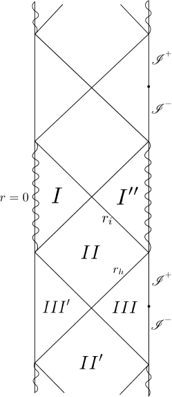
Figure 1: The Carter-Penrose diagram of (part of) the maximal analytic extension of the Reissner-Nordström AdS black hole. The union of II, II’, III and III’ fails to be globally hyperbolic due to the timelike character of $\mathcal{I}^{-}\cup\mathcal{I}^{+}$, $\mathscr{I}^{-}\cup\mathscr{I}^{+}$ which is peculiar to asymptotically anti de Sitter spaces.

For $\Lambda=0$ and $|Q|<M$, $f$ has again two positive roots $r_{i}<r_{h}$ that correspond respectively to the Cauchy and black hole horizons. In this case $f=(r-r_{i})(r-r_{h})/r^{2}$ with $Q^{2}=r_{i}r_{h}$ and $M=\tfrac{1}{2}(r_{i}+r_{h})$. The outer static region, region III in Figure 2, corresponds to $r>r_{h}$ whereas the inner static region $I$ is the one defined by $0<r<r_{i}$; the singularity at $r=0$ is covered by these two horizons. Kruskalizing at $r_{i}$ and $r_{h}$ we get further copies of these regions resulting the diagram in the figure, which extends infinitely in the vertical direction. The union of II, II’, III and III’ is globally hyperbolic, I and I’ being extensions beyond the Cauchy horizon at $r=r_{i}$, which is the future boundary of the maximum Cauchy development of initial data given at a complete spacelike hypersurface extending from spacelike infinity in region III’ to spacelike infinity in region III. In the extreme case $|Q|=M$, $r_{i}=r_{h}$ and region II collapses. For $|Q|>M$ the spacetime is not a black hole but an (unstable, see Dotti:2006gc and Dotti:2010uc ) naked singularity.

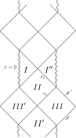
Figure 2: The Carter-Penrose diagram of (part of) the maximal analytic extension of the $|Q|<M$ Reissner-Nordström black hole. The union of II, II’, III and III’ is globally hyperbolic, its boundary at $r_{i}$ is a Cauchy horizon.

For $\Lambda>0$ we focus on the non extremal cases, for which $f$ has three simple positive roots $0<r_{i}<r_{h}<r_{c}$ which correspond to the inner, black hole and cosmological horizons respectively, and a fourth root at $r=-(r_{i}+r_{h}+r_{c})$:

$$f=-\frac{(r-r_{i})(r-r_{h})(r-r_{c})(r+r_{i}+r_{h}+r_{c})}{r^{2}(r_{i}^{2}+r_{h}^{2}+r_{c}^{2}+r_{i}r_{h}+r_{i}r_{c}+r_{h}r_{c})},$$ (104)

$Q^{2},M$ and $\Lambda$, as well as the relations among them can be found in terms of $r_{i},r_{h}$ and $r_{c}$ by comparison of (104) with (3). As before, regions separated by the horizons are numbered in increasing number for larger $r$ values. Since we can Kruskalize around all three horizons and large $r=$ constant hypersurfaces are spacelike, we get the diagram in figure 3, which extends infinitely in both directions. There are a number of extremal cases corresponding to $r_{i}=r_{h}$, $r_{h}=r_{c}$, etc, the Carter-Penrose diagrams for these cases can be found in lake .

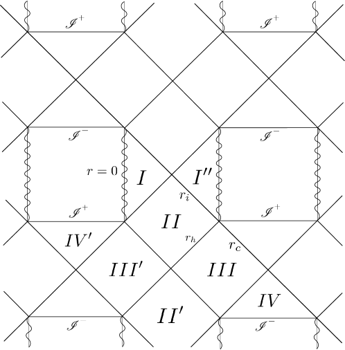
Figure 3: The Carter-Penrose diagram of (part of) the maximal analytic extension of a non extremal (three different horizons) Reissner-Nordström de Sitter black hole.

In what follows, we will prove the stability of the outer static region III of $\Lambda\geq 0$ Reissner-Nordström black holes. To this purpose, we will consider the union of regions II, II’, III and III’, which is globally hyperbolic, and study the evolution of perturbations from data on a Cauchy surface. Any Cauchy surface has two ends, one at each copy of spacelike infinity (if $\Lambda=0$) or the $r_{c}$ bifurcation sphere (if $\Lambda>0$) in regions III and III’. As explained above, we will restrict our considerations to perturbations with initial data compactly supported away from these ends. Relevant perturbations can be more general, as long as they preserve the asymptotically flat (AdS) character of the background, however, for the seek of simplicity and to allow a unified treatment of the $\Lambda=0$ and $\Lambda>0$ case we will assume compact support, as in Kay:1987ax .

Following Kay:1987ax we write (100)-(101) as

$$\partial_{t}^{2}\Phi_{n}+A_{n}\Phi_{n}=0$$ (105)

where

$$A_{n}=-\partial_{r^{*}}^{2}+V_{1}+V_{2}(-\mathbf{J}^{2})+{}_{n}{V_{3}}\;\Xi$$ (106)

and

$$V_{1}=f\Big{(}\frac{4Q^{2}}{r^{4}}-\frac{3M}{r^{3}}\Big{)}\;,V_{2}=\frac{f}{r^{2}}\;,\;{}_{n}V_{3}=(-1)^{n}\frac{f}{r^{3}}$$ (107)

are bounded functions on the outer static region $III$ for $\Lambda\geq 0$. A non trivial fact, proved in Section 6.2.1 of Kodama:2003kk is that the $A_{n},n=1,2$ are positive definite self adjoint operators in the space $L^{2}(\mathbb{R}\times S^{2},dr^{*}\sin(\theta)d\theta d\phi)$ of square integrable functions of region $III$ under this particular measure. The proof is based on a particular $S-$deformation (defined in Kodama:2003kk ) of the $A_{n}$’s.

The proof of the following Theorem is a straightforward adaptation to equation (100) of Theorem 1 in Kay:1987ax which is about the Klein Gordon equation on a Schwarzschild background . It uses the self adjointness and positive character of the $A_{n}$, $-\mathbf{J}^{2}$ and $\Xi$:

Theorem 2.

Assume $\Phi_{n}$ is a solution of equation (100) on the union of regions II, II’, III and III’ of the extended Reissner-Nordström (figure 2 or Reissner-Nordström de Sitter (figure 3) spacetimes, which has compact support on Cauchy surfaces. There exists a constant $C$ that depends on the datum of this field at a Cauchy surface, such that $|\Phi_{n}|<C$ for all points in the outer static region $III$.

Proof.

The argument in Kay:1987ax showing that we can restrict to fields that vanish at the bifurcation sphere together with its Kruskal time derivative holds here case because the $Z_{2}$ required isometry exchanging III $\leftrightarrow$ III’ is also available in this case. This implies that we may restrict our attention to fields in the outer static region decaying towards the bifurcation sphere as detailed in the Appendix in Kay:1987ax .

On a $t$ slice of region III, define the $L^{2}$ norm of a real field $G$ as

$$\lVert G\rVert^{2}=\langle G|G\rangle=\int_{\mathbb{R}\times S^{2}}G^{2}\;dr^{*}\sin(\theta)d\theta d\phi,\;\;dr^{*}=\frac{dr}{f}.$$ (108)

Note that this is not the volume element induced from the spacetime metric. The usefulness of the above norm lies in the Sobolev type inequality, equation (5.27) in dk , relating it with a point wise boundedness of $G$ on the slice

$$|G(r^{*},\theta,\phi)|\leq K\left(\lVert G\rVert+\lVert\partial_{r^{*}}^{2}G\rVert+\lVert\mathbf{J}^{2}G\rVert\right)\;,\;\;(r^{*},\theta,\phi)\in\mathbb{R}\times S^{2}$$ (109)

where $K$ is a constant. Applying this to the Regge-Wheeler fields $\Phi_{n}$ at a fixed time $t$ gives

$$|\Phi_{n}(t,r^{*},\theta,\phi)|\leq K\left(\left.\lVert\Phi_{n}\right|_{t}\rVert+\left.\lVert\partial_{r^{*}}^{2}\Phi_{n}\right|_{t}\rVert+\left.\lVert\mathbf{J}^{2}\Phi_{n}\right|_{t}\rVert\right).$$ (110)

As in the Appendix in Kay:1987ax , we will follow the strategy of proving that the $L^{2}$ norms on the right hand side of (110) can be bounded by the energies of related field configurations. Since energy is conserved for solutions of (105), we get in this way a $t-$independent upper bound of the right side of (110) and therefore, a global bound of $|\Phi_{n}(t,r^{*},\theta,\phi)|$ for all $(t,r^{*},\theta,\phi)$, i.e., of $\Phi_{n}$ in the outer static region III.

The conserved (i.e., $t-$independent) energy associated to equation (105) is

$$E=\frac{1}{2}\int_{\mathbb{R}\times S^{2}}((\partial_{t}\Phi_{n})^{2}+\Phi_{n}A_{n}\Phi_{n})\;dr^{*}\sin(\theta)d\theta d\phi.$$ (111)

Since $E$ does not depend on $t$, we may (and will) regard it as a functional on the initial datum: $E=E(\Phi^{o}_{n},\dot{\Phi}^{o}_{n})$, where $\Phi^{o}_{n}=\left.\Phi_{n}\right|_{t_{o}}$ and $\dot{\Phi}^{o}_{n}=\left.(\partial_{t}\Phi_{n})\right|_{t_{o}}$:

$$E(\Phi^{o}_{n},\dot{\Phi}^{o}_{n})=\frac{1}{2}\int_{\mathbb{R}\times S^{2}}((\dot{\Phi}^{o}_{n})^{2}+\Phi^{o}_{n}A_{n}\Phi^{o}_{n})\;dr^{*}\sin(\theta)d\theta d\phi.$$ (112)

From (106)

$$\lVert\partial_{r^{*}}^{2}\left.\Phi_{n}\right|_{t}\rVert\leq\lVert A_{n}\left.\Phi_{n}\right|_{t}\rVert+\lVert V_{1}\rVert_{\infty}\lVert\left.\Phi_{n}\right|_{t}\rVert+\lVert V_{2}\rVert_{\infty}\lVert\mathbf{J}^{2}\left.\Phi_{n}\right|_{t}\rVert+\lVert{}_{n}V_{3}\rVert_{\infty}\lVert\Xi\left.\Phi_{n}\right|_{t}\rVert,$$ (113)

where $\lVert V_{1}\rVert_{\infty}$ is the least upper bound of $V_{1}$ on the outer region III, and similarly for the other terms. Combining this with (110) gives

$$|\Phi_{n}(t,r^{*},\theta,\phi)|\leq K^{\prime}\left(\left.\lVert\Phi_{n}\right|_{t}\rVert+\lVert A_{n}\left.\Phi_{n}\right|_{t}\rVert+\left.\lVert\mathbf{J}^{2}\Phi_{n}\right|_{t}\rVert+\lVert\Xi\left.\Phi_{n}\right|_{t}\rVert\right).$$ (114)

We now use the fact that applying to a Cauchy datum $(\Phi_{n}^{o},\dot{\Phi}_{n}^{o})$ an operator that is a function of $\mathbf{J}^{2}$ or $A_{n}$ commutes with time evolution Kay:1987ax , and also use the positive definiteness of the $A_{n}$ to define $A_{n}^{\pm 1/2}$ by means of the spectral theorem. This allows us to estimate each term on the right hand side of (114) with the energy of field configurations related to the one with initial datum $(\Phi_{n}^{o},\dot{\Phi}_{n}^{o})$ (note that the first three equations below are taken verbatim from the Appendix in Kay:1987ax ),

$$\lVert\left.\Phi_{n}\right|_{t}\rVert^{2}\leq\lVert\left.\Phi_{n}\right|_{t}\rVert^{2}+\lVert A_{n}^{-\frac{1}{2}}\left.\dot{\Phi}_{n}\right|_{t}\rVert^{2}=2\;E\left(A_{n}^{-\frac{1}{2}}\Phi_{n}^{o},A_{n}^{-\frac{1}{2}}\dot{\Phi}_{n}^{o}\right),$$ (115)

$$\lVert A_{n}\left.\Phi_{n}\right|_{t}\rVert^{2}\leq\lVert A_{n}\left.\Phi_{n}\right|_{t}\rVert^{2}+\lVert A_{n}^{\frac{1}{2}}\left.\dot{\Phi}_{n}\right|_{t}\rVert^{2}=2\;E\left(A_{n}^{\frac{1}{2}}\Phi_{n}^{o},A_{n}^{\frac{1}{2}}\dot{\Phi}_{n}^{o}\right),$$ (116)

$$\lVert\mathbf{J}^{2}\left.\Phi_{n}\right|_{t}\rVert^{2}\leq\lVert\mathbf{J}^{2}\left.\Phi_{n}\right|_{t}\rVert^{2}+\lVert A_{n}^{-\frac{1}{2}}\mathbf{J}^{2}\left.\dot{\Phi}_{n}\right|_{t}\rVert^{2}=2\;E\left(A_{n}^{-\frac{1}{2}}\mathbf{J}^{2}\Phi_{n}^{o},A_{n}^{-\frac{1}{2}}\mathbf{J}^{2}\dot{\Phi}_{n}^{o}\right),$$ (117)

$$\lVert\Xi\left.\Phi_{n}\right|_{t}\rVert^{2}\leq\lVert\Xi\left.\Phi_{n}\right|_{t}\rVert^{2}+\lVert A_{n}^{-\frac{1}{2}}\Xi\left.\dot{\Phi}_{n}\right|_{t}\rVert^{2}=2\;E\left(A_{n}^{-\frac{1}{2}}\Xi\Phi_{n}^{o},A_{n}^{-\frac{1}{2}}\Xi\dot{\Phi}_{n}^{o}\right),$$ (118)

and to replace the right hand side of (114) with a time independent constant made out of the datum $(\Phi_{n}^{o},\dot{\Phi}_{n}^{o})$, as desired. ∎

Corollary 3.

Let $\mathcal{F}$ and $\mathcal{Q}$ be the fields (83) associated to a solution of the LEME. Under the assumptions of the Theorem, in the outer static region III of a $\Lambda\geq 0$ Reissner-Nordström black hole

$$\mathcal{F}<\frac{\mathcal{F}_{o}}{r^{4}},\;\;\mathcal{Q}<\frac{\mathcal{Q}_{o}}{r^{6}},$$ (119)

where $\mathcal{F}_{o}$ and $\mathcal{Q}_{o}$ are constants that depend on the Cauchy datum $(j^{(m)},A_{h}^{(m)},\dot{A}_{h}^{(m)},\Phi^{o}_{n},\dot{\Phi}^{o}_{n})$ of the perturbation.

Proof.

We use that the fields $(\mathbf{J}^{2}+2)\mathbf{J}^{2}\Phi_{n},\Xi(\mathbf{J}^{2}+2)\mathbf{J}^{2}\Phi_{2}$ and $\Xi\mathbf{J}^{2}\Phi$ that appear in (102) and (103) all satisfy equation (105) and so, according to the Theorem, are bounded by a constant. This implies that $\mathcal{F}^{>1}<\mathcal{F}_{o}^{>1}/r^{4}$, where the constant $\mathcal{F}_{o}^{>1}$ depends on the initial $\ell>1$ perturbation data, and similarly $\mathcal{Q}<\mathcal{Q}_{o}^{>1}/r^{6}$.
To see that the $\ell=1$ pieces do not spoil these bounds we use (95) and the $\ell=1$ piece of (86):

$$\mathcal{Q}^{(\ell=1)}=\frac{2(Q^{2}-Mr)}{r^{6}}\left[\frac{(3Mr-2Q^{2})}{r^{3}}\sqrt{\frac{4\pi}{3}}\sum_{m=\pm 1,0}j^{(m)}S_{(\ell=1,m)}+\frac{2Q}{r}W^{(\ell=1)}\right].$$ (120)

Each harmonic component $A_{h}^{(m)}$of $A^{(\ell=1)}_{h}=rW^{(\ell=1)}$ (equation (71)), satisfies the 1+1 wave equation (73), which is of the form of equation (1) in wald with $V$ satisfying the hypothesis used in that paper, therefore (see equation (19) in the erratum o wald ), the $A_{h}^{(m)},m=1,2,3$ are bounded, for all $t$ and $r^{*}$, by constants that depend on the initial data $(A_{h}^{(m)},\dot{A}_{h}^{(m)})$ for these fields. This gives $W^{(\ell=1)}<$ constant$/r$ which, in view of (95) and (120) implies $\mathcal{F}^{(\ell=1)}<$ constant$/r^{4}$ and $\mathcal{Q}^{(\ell=1)}<$ constant$/r^{7}$, which is consistent with (119). ∎

Theorem 1.i together with the above Corollary prove our notion of non-modal linear stability for the outer static region of $\Lambda\geq 0$ Reissner-Nordström black holes.

IV Cosmic censorship and related instabilities

The two isometric copies of the region $0<r<r_{i}$ attached to the future of $r_{i}$ are one among infinitely many different possible extensions of the spacetime beyond $r_{i}$ (although the only analytic one). For $\Lambda\geq 0$, this extension spoils the global hyperbolicity of the union of regions II, II’, III and III’ by introducing causal curves that end in the past at the $r=0$ singularity. Regions I and I’ are beyond the maximal Cauchy development of a spacelike surface extending from spacelike infinity (bifurcation sphere at $r_{c}$) in III’ to spacelike infinity (bifurcation sphere at $r_{c}$) in III in the $\Lambda=0$ ($\Lambda>0$) case. This is a complete Cauchy surface if $\Lambda=0$, and the possibility of smoothly extending the maximal future development of this surface beyond its Cauchy horizon is a rather disturbing feature of General Relativity, considered to be non generic, in a sense yet to be made precise, and referred to as the strong cosmic censorship conjecture, first proposed by Penrose almost fifty years ago penrose . The original argument given by Penrose for the $\Lambda=0$ charged black hole, is that a small amount of radiation originating outside the black hole and coming into the non static region II ($r_{i}<r<r_{h}$) is gravitationally blueshifted as it propagates inwards parallel to the Cauchy horizon, in a way such that the energy flux measured by an observer in free fall towards (the right copy, see figures 2 and 3) of region I ($0<r<r_{i}$) diverges as $r\to{r_{i}}^{+}$. This idea has proved to hold true for electro-gravitational perturbations at the linear level in chanhartle , where it was shown that for a radially free falling observer with 4-velocity $u^{a}$ the $(\ell,m)$ piece of

$$\frac{d\Phi_{n}}{d\tau}=u^{a}\nabla_{a}\Phi_{n}$$ (121)

(and therefore the complete field) diverges for $n=1,2$ as the observer approaches the Cauchy horizon. Although for some time it was thought that a positive cosmological constant introduces a competition of red and blueshifts effects that prevents this divergence in the case of nearly extremal ($r_{i}\lesssim r_{h}$) black holes Chambers:1997ef , it was later proved in Brady:1998au that if we take into account the contributions of scattered outgoing modes the divergence occurs for any positive value of $\Lambda$ allowing for a three horizon structure. Further evidence of the instability of the Cauchy horizon are Poisson:1990eh and related works, as well as more recent models including a scalar field (to avoid Birkhoff’s theorem), see Burko:2002fv and Maeda:2005yd .
The Regge-Wheeler-Zerilli potentials $\Phi_{n}$ in equation (121), whose derivative with respect to proper time is shown to diverge at the Cauchy horizon in chanhartle for $\Lambda=0$ and for $\Lambda>0$ in Brady:1998au are, of course, non observable, as they are potentials for the metric and electromagnetic field perturbations, although the square of (121) contributes to the flux of energy of the perturbation. However, the $\Phi_{n}$ enter the harmonic expansion of the $\ell>1$ pieces of $\mathcal{Q}$ and $\mathcal{F}$, and the implications of the combined set of equations (102), (103) and (121) are immediate: for a radially infalling observer crossing $r_{i}$, the rate $dr/d\tau$ is clearly nonzero and finite. For such an observer, $d/d\tau=u^{c}\nabla_{c}$ commutes with the angular operators $\mathbf{J}^{2}$ and $\Xi$. This implies that both $d\mathcal{F}_{>1}/d\tau$ and $d\mathcal{Q}_{>1}/d\tau$ will diverge along this geodesic as $r\to r_{i}^{+}$ (and so will diverge $d\mathcal{F}/d\tau$ and $d\mathcal{Q}/d\tau$), suggesting that the Cauchy horizon is replaced with a curvature singularity. Of course, this statement needs to be taken with care since as soon as $r_{i}$ is approached and these quantities start to grow, the linearized equations become useless an one needs to study the evolution of the perturbation using other techniques; but in any case the divergence at $r_{i}$ of the linear fields is a clear indication of strong cosmic censorship.

The extreme case $r_{i}=r_{h}$ has been less studied, although it was recently shown that for $\Lambda=0$ (case in which the extreme black holes corresponds to $|Q|=M=r_{i}=r_{h}$) the transverse derivative $\partial\Phi_{n}/\partial r$ in coordinates $(v=t+r^{*},r,\theta,\phi)$ (again, for a fixed $\ell$ component) diverges at $r=r_{i}$ as $v\to\infty$ along the horizon null generators Lucietti:2012xr . The divergence follows from a set quantities that are shown from (100) to be conserved along the $r_{i}=r_{h}$ horizon generators. These are analogous to a similar set of conserved quantities for the massless scalar wave equation found in Aretakis:2012ei , the conservation of which was shown in Bizon:2012we to follow from a combination of Newman Penrose conserved quantities at null infinity newmanpenrose and a conformal discrete isometry that exchanges the degenerate horizon and null infinity, isometry discovered in couch and used in Dain:2012qw to explain the symmetry of the effective potential and the consistency of the pointwise bounds for a massles scalar field in the extreme case.
Perturbations of the extreme $\Lambda=0$ case were studied non linearly in a recent paper by Reiris Reiris:2014xca where it was shown that small electro-vacuum perturbations of initial data of extreme Reissner-Nordström black holes cannot decay in time into an extreme Kerr-Newman black hole. The evidence in Reiris:2014xca is that these non-stationary solutions of the Einstein-Maxwell equations will settle into a sub-extremal black hole of the Kerr-Newman family.

As a final comment we mention that, besides the strong evidence supporting the idea that a slightly perturbed Reissner-Nordström black hole will develop a curvature singularity that cuts off the innermost region I ($0<r<r_{i}$), this non-unique extension beyond $r_{i}$ is by itself linearly unstable under electro-gravitational perturbations Dotti:2010uc . The instability, confined to this region, belongs to the even sector of the linear perturbations.

V Discussion

We proved that the odd sector of Einstein-Maxwell perturbations around a Reissner-Nordström (A)dS black hole shares with the uncharged Schwarzschild black hole the property that there are physically meaningful, gauge invariant scalar fields $\mathcal{Q}$ and $\mathcal{F}$ encoding the same information as a gauge class of a metric perturbation and satisfying a system of four dimensional wave equations which are entirely equivalent to the linearized Einstein-Maxwell equations. For uncharged black holes $Q=0$ the system of equations decouple, leaving the equation found in Dotti:2013uxa Dotti:2016cqy for the gravitational degrees of freedom, encoded in $\mathcal{Q}$, and the Fackerrel Ipser equation for the Maxwell degrees of freedom $\mathcal{F}$.
Besides the significant reduction of the linearized Einstein-Maxwell system to scalar field equations, the resulting system of equations allow us to prove that, for generic perturbations, $\mathcal{Q}$ and $\mathcal{F}$ are pointwise bounded in the outer static region. This gives a strong notion of linear stability in this region, analogous to that found in Dotti:2013uxa and Dotti:2016cqy for the Schwarzschild black hole.

If we assume that the large $t$ decay at fixed $r$ of solutions of the Regge-Wheeler equation in the $Q=0$ case (known as Price tails, see Price:1971fb , and Brady:1996za for $\Lambda>0$) occurs also for the $Q\neq 0$ Regge-Wheeler fields $\Phi_{n}$ in (105), and note that equation (73) for $A_{h}^{(m)}$ formally agrees with the Regge-Wheeler equation (100)-(101) for $n=1$ and $\ell=1$ (as suggested by (98)) and so also decays for large $t$, we conclude, using the 1-1 correspondence between odd perturbations and the set of $(\mathcal{Q},\mathcal{F})$’s, together with equations (85), (86), (98) and (99), that at large $t$

$$\mathcal{F}\simeq\frac{8Q^{2}}{r^{5}}\sqrt{\frac{4\pi}{3}}\sum_{m=\pm 1,0}j^{(m)}S_{(\ell=1,m)},$$ (122)

and

$$\mathcal{Q}\simeq\frac{2(Q^{2}-Mr)(3Mr-2Q^{2})}{r^{9}}\sqrt{\frac{4\pi}{3}}\sum_{m=\pm 1,0}j^{(m)}S_{(\ell=1,m)},$$ (123)

which corresponds to a deformation within the Kerr-Newman (Kerr-Newman de Sitter) family by adding a small amount of angular momentum. This is consistent with the picture that the perturbed black hole settles at large times into a slowly rotating charged black hole.

The divergence of $d\mathcal{F}/d\tau$ and $d\mathcal{Q}/d\tau$ for free falling radial observers as they approach the Cauchy horizon from region II, proved in the previous Section, supports strong cosmic censorship in its purest form, as $\mathcal{Q}$ is a perturbed curvature scalar. This result, however, has to be taken with caution, as the linear perturbation scheme becomes less reliable as linear fields grow.

VI Acknowledgements

This work was partially funded by grants PIP 11220080102479 (Conicet-Argentina) and 30720110101569CB (Universidad Nacional de Córdoba). J.M.F.T. is supported by a fellowship from Conicet.

References

• (1) G. Dotti, “Nonmodal linear stability of the Schwarzschild black hole,” Phys. Rev. Lett.  112, 191101 (2014),
• (2) H. Kodama and A. Ishibashi, “Master equations for perturbations of generalized static black holes with charge in higher dimensions,” Prog. Theor. Phys.  111, 29 (2004) [hep-th/0308128].
• (3) G. Dotti, “Black hole nonmodal linear stability: the Schwarzschild (A)dS cases,” Class. Quant. Grav.  33, 205005 (2016), arXiv:1603.03749 [gr-qc]. [arXiv:1307.3340 [gr-qc]].
• (4) T. Regge and J. A. Wheeler, “Stability of a Schwarzschild singularity,” Phys. Rev.  108, 1063 (1957). doi:10.1103/PhysRev.108.1063
• (5) F. J. Zerilli, “Effective potential for even parity Regge-Wheeler gravitational perturbation equations,” Phys. Rev. Lett.  24, 737 (1970). doi:10.1103/PhysRevLett.24.737
• (6) F. J. Zerilli, “Perturbation analysis for gravitational and electromagnetic radiation in a Reissner-Nordström geometry.” Phys. Rev. D 9, 860 (1974).
• (7) A. Ishibashi and H. Kodama, “Perturbations and Stability of Static Black Holes in Higher Dimensions,” Prog. Theor. Phys. Suppl.  189, 165 (2011) [arXiv:1103.6148 [hep-th]].
• (8) V. Moncrief, “Odd-parity stability of a Reissner-Nordstrom black hole,” Phys. Rev. D 9, 2707 (1974).
• (9) V. Moncrief, “Stability of Reissner-Nordstrom black holes,” Phys. Rev. D 10, 1057 (1974).
• (10) V. Moncrief, “Gauge-invariant perturbations of Reissner-Nordstrom black holes,” Phys. Rev. D 12, 1526 (1975).
• (11) R. Wald, “Note on the stability of the Schwarzschild metric”, J. Math. Phys. 20, 1056 (1979), Erratum J. Math. Phys. 21, 218 (1980).
• (12) E. Chaverra, N. Ortiz and O. Sarbach, “Linear perturbations of self-gravitating spherically symmetric configurations,” Phys. Rev. D 87, no. 4, 044015 (2013) [arXiv:1209.3731 [gr-qc]].
• (13) A. Ishibashi and R. M. Wald, “Dynamics in nonglobally hyperbolic static space-times. 3. Anti-de Sitter space-time,” Class. Quant. Grav.  21, 2981 (2004) [hep-th/0402184].
• (14) O. Sarbach and M. Tiglio, “Gauge invariant perturbations of Schwarzschild black holes in horizon penetrating coordinates,” Phys. Rev. D 64, 084016 (2001) doi:10.1103/PhysRevD.64.084016 [gr-qc/0104061].
• (15) G. W. Gibbons and S. W. Hawking, “Cosmological Event Horizons, Thermodynamics, and Particle Creation,” Phys. Rev. D 15, 2738 (1977). doi:10.1103/PhysRevD.15.2738
• (16) See http://grtensor.phy.queensu.ca/
• (17) E. D. Fackerell and J. R. Ipser, “Weak electromagnetic fields around a rotating black hole,” Phys. Rev. D 5, 2455 (1972). doi:10.1103/PhysRevD.5.2455
• (18) J. Jezierski and T. Smołka, “A geometric description of Maxwell field in a Kerr spacetime,” Class. Quant. Grav.  33, no. 12, 125035 (2016) [arXiv:1502.00599 [gr-qc]].
• (19) B. Araneda and G. Dotti, “Instability of asymptotically anti de Sitter black holes under Robin conditions at the timelike boundary,” arXiv:1611.03534 [hep-th].
• (20) B. S. Kay and R. M. Wald, “Linear Stability Of Schwarzschild Under Perturbations Which Are Nonvanishing On The Bifurcation Two Sphere,” Class. Quant. Grav.  4, 893 (1987).
• (21) Dimock J. and Kay B. S., “Classical and quantum scattering theory for linear scalar fields on the Schwarzschild metric I”, Annals of Physics, 175 (1987), 366.
• (22) R. H. Price, “Nonspherical perturbations of relativistic gravitational collapse. 1. Scalar and gravitational perturbations,” Phys. Rev. D 5, 2419 (1972). doi:10.1103/PhysRevD.5.2419.
• (23) K. Lake, “Reissner-Nordstrom-de Sitter metric, the third law, and cosmic censorship”, Phys. Rev. D 19, 421 (1979).
• (24) P. R. Brady, C. M. Chambers, W. Krivan and P. Laguna, “Telling tails in the presence of a cosmological constant,” Phys. Rev. D 55, 7538 (1997) doi:10.1103/PhysRevD.55.7538 [gr-qc/9611056].
• (25) S. Chandrasekhar, “On algebraically special perturbations of black holes”, Proc. R. Soc. Lond. A 392 (1984) 1.
• (26) S. Chandrasekhar, “The Mathematical Theory of Black Holes”, Oxford University Press, second edition, 1992.
• (27) R. Penrose, in Battelle Rencontres, edited by C. de Witt and J.A. Wheeler (W.A. Benjamin, New York, 1968), p. 222.
• (28) S. Chandrasekhar and J. B. Hartle, “On Crossing the Cauchy Horizon of a Reissner-Nordstrom Black-Hole”, Proceedings of the Royal Society of London. A 384 (1982), 301.
• (29) C. M. Chambers, “The Cauchy horizon in black hole de sitter space-times,” Annals Israel Phys. Soc.  13, 33 (1997) [gr-qc/9709025].
• (30) P. R. Brady, I. G. Moss and R. C. Myers, “Cosmic censorship: As strong as ever,” Phys. Rev. Lett.  80, 3432 (1998) doi:10.1103/PhysRevLett.80.3432 [gr-qc/9801032].
• (31) G. Dotti, R. Gleiser and J. Pullin, “Instability of charged and rotating naked singularities,” Phys. Lett. B 644, 289 (2007) doi:10.1016/j.physletb.2006.12.004 [gr-qc/0607052].
• (32) G. Dotti and R. J. Gleiser, “Gravitational instability of the inner static region of a Reissner-Nordstrom black hole,” Class. Quant. Grav.  27, 185007 (2010) doi:10.1088/0264-9381/27/18/185007 [arXiv:1001.0152 [gr-qc]].
• (33) E. Poisson and W. Israel, “Internal structure of black holes,” Phys. Rev. D 41, 1796 (1990). doi:10.1103/PhysRevD.41.1796
• (34) L. M. Burko, “Black hole singularities: A New critical phenomenon,” Phys. Rev. Lett.  90, 121101 (2003) Erratum: [Phys. Rev. Lett.  90, 249902 (2003)] doi:10.1103/PhysRevLett.90.121101 [gr-qc/0209084].
• (35) H. Maeda, T. Torii and T. Harada, “Novel Cauchy-horizon instability,” Phys. Rev. D 71, 064015 (2005) doi:10.1103/PhysRevD.71.064015 [gr-qc/0501042].
• (36) J. Lucietti, K. Murata, H. S. Reall and N. Tanahashi, “On the horizon instability of an extreme Reissner-Nordstróm black hole,” JHEP 1303, 035 (2013) doi:10.1007/JHEP03(2013)035 [arXiv:1212.2557 [gr-qc]].
• (37) S. Aretakis, “Horizon Instability of Extremal Black Holes,” Adv. Theor. Math. Phys.  19, 507 (2015) doi:10.4310/ATMP.2015.v19.n3.a1 [arXiv:1206.6598 [gr-qc]].
• (38) P. Bizon and H. Friedrich, “A remark about wave equations on the extreme Reissner-Nordstróm black hole exterior,” Class. Quant. Grav.  30, 065001 (2013) doi:10.1088/0264-9381/30/6/065001 [arXiv:1212.0729 [gr-qc]].
• (39) E. T. Newman and R. Penrose, “New conservation laws for zero rest-mass fields in asymptotically flat spacetime”, Proc. R. Soc. London, Ser. A 305, 175204 (1968).
• (40) Couch W. and Torrence R., “Conformal invariance under spatial inversion of extreme Reissner–Nordström black holes”, Gen. Rel. Grav. 16 (1984), 789.
• (41) S. Dain and G. Dotti, “The wave equation on the extreme Reissner-Nordstróm black hole,” Class. Quant. Grav.  30, 055011 (2013) doi:10.1088/0264-9381/30/5/055011 [arXiv:1209.0213 [gr-qc]].
• (42) M. Reiris, “On Perturbations of Extreme Kerr–Newman Black Holes and their Evolution,” Annales Henri Poincare 16, no. 7, 1551 (2015).