Duration of classicality in highly degenerate interacting Bosonic systems

Abstract

We study sets of oscillators that have high quantum occupancy and that interact by exchanging quanta. It is shown by analytical arguments and numerical simulation that such systems obey classical equations of motion only on time scales of order their relaxation time $\tau$ and not longer than that. The results are relevant to the cosmology of axions and axion-like particles.

The question under consideration here is: on what time scale do highly degenerate, interacting quantum oscillators obey classical equations of motion? Consider the broad class of systems that have a Hamiltonian of the form

$$H=\sum_{j}\omega_{j}a_{j}^{\dagger}a_{j}+{1\over 4}\sum_{jkln}\Lambda_{jk}^{ln}a_{j}^{\dagger}a_{k}^{\dagger}a_{l}a_{n}$$ (1)

where the $a_{j}$ and $a_{j}^{\dagger}$ are annihilation and creation operators satisfying canonical equal-time commutation relations. ${\cal N}_{j}=a_{j}^{\dagger}a_{j}$ is the number of quanta in oscillator $j$. For the sake of definiteness, we have restricted ourselves in Eq. (1) to systems in which the total number of quanta $N=\sum_{j}{\cal N}_{j}$ is conserved. The system states are given by linear combinations

$$|\Psi(t)\rangle=\sum_{\{{\cal N}_{j}\}}c(\{{\cal N}_{j}\},t)~{}|\{{\cal N}_{j}\}\rangle$$ (2)

of eigenstates $|\{{\cal N}_{j}\}\rangle$ of the ${\cal N}_{j}$ for arbitrary distributions $\{{\cal N}_{j}\}=({\cal N}_{1},{\cal N}_{2},{\cal N}_{3},...)$ of the quanta over the oscillators. In the Heisenberg picture, where the time-dependence of the state vectors has been removed, the annihilation operators $a_{j}(t)$ satisfy the equations of motion

$$i\dot{a}_{j}=[a_{j},H]=\omega_{j}a_{j}+{1\over 2}\sum_{kln}\Lambda_{jk}^{ln}a_{k}^{\dagger}a_{l}a_{n}~{}~{}\ .$$ (3)

The classical description of the system is obtained by replacing the $a_{j}(t)$ with c-numbers $A_{j}(t)$. They satisfy

$$i\dot{A}_{j}=\omega_{j}A_{j}+{1\over 2}\sum_{kln}\Lambda_{jk}^{ln}A_{k}^{*}A_{l}A_{n}~{}~{}\ .$$ (4)

The quantum description always requires vastly more information than the classical one. To be specific, if the number of oscillators is $M$ and the number of quanta $N$, the classical state is given by $2M-1$ real numbers, whereas the quantum state is given by

$$D={(N+M-1)!\over N!(M-1)!}-1$$ (5)

complex numbers. For example, if $N=100$ and $M=10$, $D=4.26\cdot 10^{12}$. $D$ increases extremely fast with increasing $N$ and $M$. Clearly a huge simplification occurs if the system obeys classical equations of motion. The question is: when is this approximation valid?

The question is particularly relevant to axion cosmology axdm ; CABEC ; axtherm ; Saikawa ; Berges ; Guth . The number of axions inside a co-moving volume of size (1 Mpc)³ today is $N\simeq 4\cdot 10^{81}$, assuming all the dark matter is axions and the axion mass is $10^{-5}$ eV. Before structure formation, their momentum dispersion is at most of order $\delta p\sim{1\over t_{1}}{a(t_{1})\over a(t)}$ where $t_{1}\sim 10^{-7}$ sec is the age of the universe when the axion mass effectively turns on, and $a(t)$ is the cosmological scale factor. Their quantum degeneracy, i.e. the average occupation number of those states that the axions occupy, is thus at least of order ${\cal N}\sim 10^{61}$ CABEC . Almost all discussion of the cosmology of axions axdm ; Guth ; Braaten or axion-like ALPs particles assumes that the axion fluid obeys classical field equations. However, it was shown in refs. CABEC ; axtherm that the axion fluid thermalizes on a time scale shorter than the age of the universe after the photon temperature has dropped below approximately 500 eV. When the axion fluid thermalizes, it satisfies all conditions for Bose-Einstein condensation and this should therefore be the expected outcome on theoretical grounds. Furthermore it was shown case that Bose-Einstein condensation of cold dark matter axions explains precisely and in all respects the observational evidence for caustic rings of dark matter in disk galaxies. The evidence is summarized in ref. Duffy . Bose-Einstein condensation is a quantum effect. The argument that cold dark matter axions form a Bose-Einstein condensate was questioned Guth in part on the belief that the cosmic axion fluid satisfies classical field equations as a result of its extremely high degeneracy. This belief is also implicit in the many other discussions of dark matter axions, or axion-like particles, which describe the axion fluid by classical field equations ALPs . So, we want to ask: is it true that highly degenerate Bosonic systems obey classical equations of motion merely because they are highly degenerate? And, if they obey classical field equations of motion for a while but not forever, what is the time scale over which classical equations of motion are obeyed?

When the interactions among the oscillators are turned off, i.e. when the $\Lambda_{jk}^{ln}=0$, and the degeneracy ${\cal N}$ is high, a classical description is in fact correct, and accurate to order $1/{\cal N}$. Indeed Eqs. (3) and (4) are linear in that case and admit solutions that have identical time dependence. If the expected values $\langle{\cal N}_{j}\rangle\equiv\langle\Psi(t)|{\cal N}_{j}|\Psi(t)\rangle$ and their classical analogues $N_{j}=A_{j}^{*}(t)A_{j}(t)$ are equal initially, they remain equal ever after. In spite of its apparent “triviality”, the non-interacting case describes a large number of interesting phenomena where the system has a non-trivial evolution either because the initial state is a linear superposition of different eigenmodes (e.g. the beating of a double pendulum) or because the oscillation frequencies of the oscillators are time-dependent (e.g. parametric resonance). Such phenomena are described by classical physics when ${\cal N}$ is large. The production of cold axions by vacuum realignment in the early universe is a case in point. Because the effect is due to the time dependence of the axion mass and interactions do not play an important role, a classical physics calculation produces a correct estimate of the axion cosmological energy density from vacuum realignment axdm . Perhaps the successes of classical physics when $\Lambda_{jk}^{ln}=0$ and ${\cal N}\rightarrow\infty$ has led to a widely held belief that classical physics also gives a good description when $\Lambda_{jk}^{ln}\neq 0$ and ${\cal N}\rightarrow\infty$.

When $\Lambda_{jk}^{ln}\neq 0$, the $\langle{\cal N}_{j}\rangle$ are time-dependent because quanta jump between oscillators in pairs: one quantum jumps from oscillator $l$ to oscillator $j$ while another quantum jumps from $n$ to $k$. The classical $N_{j}(t)$ are also time-dependent when $\Lambda_{jk}^{ln}\neq 0$. The question here is whether the time dependence is the same. Assuming the initial state is far from equilibrium, there exists a time scale $\tau$ over which the distribution of the quanta over the oscillators changes completely, i.e. each $\langle{\cal N}_{j}\rangle$ changes by order 100%. We call $\tau$ the relaxation time and $\Gamma=1/\tau$ the relaxation rate. If the system is stable, it will move toward thermal equilibrium on a time scale of order $\tau$. If the system is unstable, it will also move towards thermal equilibrium on a time scale of order $\tau$ provided the time scale of instability is long compared to $\tau$.

There is a simple a-priori reason to expect the quantum and classical descriptions to deviate from each other on a time scale of order $\tau$. Indeed, the quantum description has the system move towards a Bose-Einstein distribution whereas the classical description has the system move towards a Boltzmann distribution. This argument is compelling but perhaps not precise enough to give us an estimate of the time scale of classicality. It allows the classical description to be valid, for example, on a time scale of order $\tau\log({\cal N})$. For the systems that we are familiar with in the laboratory, mainly superfluid ⁴He and dilute ultra-cold atoms, the quantum degeneracy is not much larger than one. So we have no compelling guidance from experiment to tell us about the behavior of systems with huge degeneracy such as the cosmic axion fluid with ${\cal N}\sim 10^{61}$.

To gain insight, consider the evolution equations for the occupation numbers. There are two cases to consider depending whether $\Gamma<\delta\omega$, where $\delta\omega$ is the energy dispersion, or $\Gamma>\delta\omega$. In the first case, called the particle kinetic regime, we have

$$\dot{\cal N}_{j}=\sum_{kln}|\Lambda_{jk}^{ln}|^{2}\pi\delta(\omega_{j}+\omega_{k}-\omega_{l}-\omega_{n})\cdot~{}~{}~{}$$

$$\cdot[({\cal N}_{j}+1)({\cal N}_{k}+1){\cal N}_{l}{\cal N}_{n}-{\cal N}_{j}{\cal N}_{k}({\cal N}_{l}+1)({\cal N}_{n}+1)]$$ (6)

for the operators ${\cal N}_{j}(t)$ in the Heisenberg picture axtherm , and

$$\dot{N}_{j} = \sum_{kln}|\Lambda_{jk}^{ln}|^{2}\pi\delta(\omega_{j}+\omega_{k}-\omega_{l}-\omega_{n})\cdot$$ (7)

$$\cdot [(N_{k}+N_{j})N_{l}N_{n}-N_{k}N_{j}(N_{l}+N_{n})]$$

for the c-numbers $N_{j}(t)$ premature . In the second case, called the condensed regime, we have instead axtherm

$$\dot{\cal N}_{j}={i\over 2}\sum_{kln}(\Lambda_{ln}^{jk}a_{l}^{\dagger}a_{n}^{\dagger}a_{k}a_{j}-\Lambda_{jk}^{ln}a_{j}^{\dagger}a_{k}^{\dagger}a_{l}a_{n})$$ (8)

and

$$\dot{N}_{j}={i\over 2}\sum_{kln}(\Lambda_{ln}^{jk}A_{l}^{*}A_{n}^{*}A_{j}A_{k}-\Lambda_{jk}^{ln}A_{j}^{*}A_{k}^{*}A_{l}A_{n})~{}~{}\ .$$ (9)

For a fluid of interacting particles, such as the cosmic axion fluid, the oscillators in Eq. (1) are labeled by the particle momenta $\vec{p}={2\pi\over L}(n_{1},n_{2},n_{3})$ where the $n_{r}$ ($r$ = 1,2,3) are integers and $L$ is the linear size of a large cubic volume $V=L^{3}$ in which the associated quantum field satisfies periodic boundary conditions. The oscillator frequencies are $\omega_{\vec{p}}={p^{2}\over 2m}$ in the non-relativistic limit. In the case of cosmic axions, the relevant interactions are $\lambda\phi^{4}$ and gravitational, for which the couplings are respectively

$$\Lambda_{\lambda~{}\vec{p}_{1},\vec{p}_{2}}^{\vec{p}_{3},\vec{p}_{4}}={\lambda\over 4m^{2}V}\delta_{\vec{p}_{1}+\vec{p}_{2},\vec{p}_{3}+\vec{p}_{4}}$$ (10)

and

$$\Lambda_{g~{}\vec{p}_{1},\vec{p}_{2}}^{\vec{p}_{3},\vec{p}_{4}}=-{4\pi Gm^{2}\over V}({1\over|\vec{p}_{1}-\vec{p}_{3}|^{2}}+{1\over|\vec{p}_{1}-\vec{p}_{4}|^{2}})\delta_{\vec{p}_{1}+\vec{p}_{2},\vec{p}_{3}+\vec{p}_{4}}~{}~{}\ .$$ (11)

In the particle kinetic regime, Eqs. (6) and (7) imply relaxation rates of order

$$\Gamma_{\rm pk}\sim n\sigma\delta v{\cal N}$$ (12)

where $n$ is the physical space density, $\delta v$ is the velocity dispersion, and $\sigma$ is the appropriate cross-section. For $\lambda\phi^{4}$ interactions, $\sigma_{\lambda}={\lambda^{2}\over 64\pi m^{2}}$. For gravity, the appropriate cross-section is that for large angle scattering, $\sigma_{g}\sim{4G^{2}m^{2}\over(\delta v)^{4}}$, since forward scattering does not contribute to relaxation. In the condensed regime, Eqs. (8) and Eqs. (9) imply relaxation rates of order

$$\Gamma_{{\rm cr},\lambda}\sim{n\lambda\over 4m^{2}}~{}~{}~{}{\rm and}~{}~{}~{}\Gamma_{{\rm cr},g}\sim{4\pi Gn\over(\delta v)^{2}}$$ (13)

respectively. The relaxation rate estimates appear very different in the two regimes. However they are related by $\Gamma_{\rm pk}\sim(\Gamma_{\rm cr})^{2}/\delta\omega$ so that they agree with one another at the inter-regime boundary where $\Gamma=\delta\omega$. Axion dark matter was found CABEC ; axtherm to thermalize in the condensed regime by their gravitational self-interactions when the photon temperture is of order 500 eV.

Eqs. (6) and (8) for quantum evolution closely resemble their classical counterparts, Eqs. (7) and (9). However, let us point out two significant differences between Eqs. (6) and (7). Similar differences exist between Eqs. (8) and (9). The first and, as it will turn out, most important difference is that Eq. (6) is an operator equation whereas Eq. (7) is a c-number equation. The second difference is that the expression in brackets in Eq. (6) has terms ${\cal N}_{l}{\cal N}_{n}-{\cal N}_{j}{\cal N}_{k}$ that have no analogues in Eq. (7). Indeed, if one attempts to derive Eq. (7) from (6) by taking the quantum expectation value on both sides of Eq. (6) and identifying $\langle{\cal N}_{j}(t)\rangle$ with $N_{j}(t)$, one encounters two difficulties. The first is that $\langle{\cal N}_{j}{\cal N}_{k}{\cal N}_{l}\rangle\neq\langle{\cal N}_{j}\rangle\langle{\cal N}_{k}\rangle\langle{\cal N}_{l}\rangle$. The second is that the expressions in brackets in the two equations are different even after replacing ${\cal N}_{j}$ by $N_{j}$.

There are specific cases where Eqs. (6) and (7) make dramatically different predictions because of the quadratic terms in Eq. (6) that have no analogues in Eq. (7). For example consider the initial momentum distribution

$$N_{\vec{p}}=\sum_{j=1}^{J}N_{j}\delta_{\vec{p},\vec{p}_{j}}$$ (14)

with $N_{j}\neq 0$ for a set of momenta $\vec{p}_{j}$ ($j=1,2,...,J)$ such that the process $\vec{p}+\vec{p}^{~{}\prime}\rightarrow\vec{p}^{~{}\prime\prime}+\vec{p}^{`\prime\prime\prime}$ violates energy-momentum conservation for any $\vec{p}$, $\vec{p}^{~{}\prime}$ and $\vec{p}^{~{}\prime\prime}$ belonging to the set, and arbitrary $\vec{p}^{~{}\prime\prime\prime}$. In other words, in this configuration any scattering allowed by energy-momentum conservation is into final states that are both initially empty. This momentum distribution has a time-dependent evolution according to Eq. (6), whereas it is time-independent according to Eq. (7). Indeed the process $\vec{p}+\vec{p}^{~{}\prime}\rightarrow\vec{p}^{~{}\prime\prime}+\vec{p}^{~{}\prime\prime\prime}$ always occurs in the quantum theory when the initial modes are occupied (${\cal N}_{\vec{p}}\neq 0$ and ${\cal N}_{{\vec{p}}^{~{}\prime}}\neq 0$), whereas it occurs in the classical theory only if in addition one of the final modes is occupied ($N_{\vec{p}^{~{}\prime\prime}}\neq 0$ or $N_{\vec{p}^{~{}\prime\prime\prime}}\neq 0$). As a particular case, two monochromatic particle beams do not scatter in the classical theory unless one of the final states allowed by energy-momentum conservation is already occupied, whereas two such beams always scatter in the quantum theory. The momentum distribution of Eq. (14) is not generic but even for generic initial momentum distributions the $\langle{\cal N}_{j}\rangle$ will deviate from the $N_{j}$ because of the extra terms in the brackets of Eq. (6) that have no analogues in Eq. (7). After a time of order $\tau$, the resulting difference $\langle{\cal N}_{j}\rangle-N_{j}$ will be ${\cal O}(1)$ and then grow exponentially fast as the quantum evolution leads to a Bose-Einstein distribution whereas the classical evolution leads to a Boltzmann distribution. So the classical evolution will certainly deviate from the quantum evolution by order 100% after a time of order $\tau\log{\cal N}$. Actually, as we now show, the classical and quantum evolutions deviate from one another much faster than that because Eq. (6) is an operator equation whereas Eq. (7) is a c-number equation.

Only in eigenstates $|\{{\cal N}_{j}\}\rangle$ of the occupation numbers is $\langle{\cal N}_{j}{\cal N}_{k}{\cal N}_{l}\rangle=\langle{\cal N}_{j}\rangle\langle{\cal N}_{k}\rangle\langle{\cal N}_{l}\rangle$. Generally speaking, it is exceedingly unlikely at any given moment that the quantum state is an eigenstate of the occupation numbers. Even if it happens to be in such a state, quantum evolution will soon, as a result of interactions, cause it to become a linear superposition of many different $|\{{\cal N}_{j}\}\rangle$. In contrast, the classical state is always an eigenstate of the $N_{j}$. To investigate the implications of this difference, we carried out numerical simulations of five oscillators in the condensed regime. The toy system we use was first described in ref. axtherm and shown there to thermalize on the expected time scale $\tau$. Its Hamiltonian has the form given in Eq. (1) with $\omega_{j}=j\omega_{1}$ ($j$ = 1, 2, 3, 4, 5) and $\Lambda_{jk}^{ln}=0$ unless $j+k=l+n$. Non-zero values are given to $\Lambda_{14}^{23}$, $\Lambda_{15}^{24}$, $\Lambda_{25}^{34}$, $\Lambda_{22}^{13}$, $\Lambda_{33}^{24}$, $\Lambda_{33}^{15}$ and $\Lambda_{44}^{35}$, and their conjugates $\Lambda_{jk}^{ln}=\Lambda_{ln}^{jk~{}*}$. We numerically integrate the Schrödinger equation

$$i\partial_{t}|\Psi(t)\rangle=H|\Psi(t)\rangle$$ (15)

for this model starting from an initial state which is an eigenstate of the occupation numbers, calculate the expectation values $\langle{\cal N}_{j}\rangle(t)$ and compare with the classical evolution $N_{j}(t)$ obtained by numerically integrating Eqs. (4). A large number of initial conditions were simulated. We find in all cases that the classical evolution deviates from the quantum evolution on a time scale which is short compared to $\tau$.

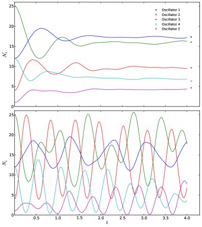
Figure 1: Quantum (top) and classical (bottom) time evolution of the occupation numbers in the toy system described in the text for the initial state $|12,25,4,12,1\rangle$. The dots on the right in the top panel indicate the thermal averages in the quantum case. The quantum system approaches the thermal averages on the expected time scale. The classical system does not equilibrate. The classical evolution tracks the quantum evolution only very briefly.

The top panel of Fig. 1 shows the quantum evolution of the initial state $|{\cal N}_{1},{\cal N}_{2},...,{\cal N}_{5}\rangle=|12,25,4,12,1\rangle$ as an example. The figure shows that the expected values $\langle{\cal N}_{j}\rangle$ move towards the thermal averages on the expected time scale $\tau$, which is of order one given the coupling strengths $\Lambda_{jk}^{ln}$ in the simulation axtherm . The quantum thermal averages are computed by giving equal probability to each system state consistent with the total number of quanta and the total energy in the initial state. They are shown by the dots on the right side of Fig. 1. The bottom panel of Fig. 1 shows the classical evolution of the initial state $(A_{1},A_{2},...,A_{5})=(\sqrt{12},\sqrt{25},\sqrt{4},\sqrt{12},\sqrt{1})$, in which the $N_{j}$ and their time derivatives $\dot{N}_{j}$ have the same initial values as their quantum analogues in the top panel. Fig. 1 shows that the classical evolution tracks the quantum evolution only for a short time compared to $\tau$. Fig. 1 also shows that the classical oscillators do not approach thermal equilibrium on the time scale $\tau$. If the simulation is prolonged, one finds that the classical oscillators do not thermalize even after a very long time. This phenomenon was first noted by Fermi, Pasta and Ulam in 1955 and has been studied by many authors since Fermi .

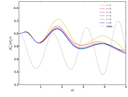
Figure 2: Quantum evolution of the occupation number of the fourth oscillator (solid lines) of the toy system when the initial occupation numbers are $r\times$(6,4,5,4,3) with $r=1,2,...6$. Both axes are rescaled according to the scale invariance of the classical equations of motion. The classical evolution is shown by the dotted line. The figure shows that when $r$ is increased, the quantum evolution approaches a limit which differs from the classical evolution.

Our concern is whether the classical evolution is a good approximation to the quantum evolution. It is not for the initial condition described in the previous paragraph, nor for all the other initial conditions that we simulated. One may wonder whether this due to the occupation numbers being too small. To test this we did a series of simulations in which all the occupation numbers are scaled up by a common factor $r$. The classical evolution remains unchanged under such a rescaling provided time $t$ is rescaled by $1/r$. The quantum evolution is not rescaling invariant for small $r$ but is found in our simulations to approach a rescaling invariant limit when $r$ is increased, as shown in Fig. 2. For the largest system simulated (r=6), the occupation numbers range from 18 to 36. Performing much larger simulations is prohibitively expensive. However, the convergence of the quantum behaviour for increasing r leads us to believe that a further increase of the occupation numbers would not produce any relevant changes. Thus we find that the quantum evolution is different from the classical evolution in the large ${\cal N}$ limit.

One may also ask whether the classical evolution equations give a good approximation to quantum evolution if the initial state is a coherent state, i.e. a state of minimum uncertainty in the $a_{j}$. We tested this and found that it does not. Fig. 3 shows three different evolutions of the initial state (0,12,16,0,0): i) the classical evolution, ii) the quantum evolution, and iii) the quantum evolution of the corresponding coherent state. Evolutions ii) and iii) are similar and different from evolution i).

We conclude that highly degenerate interacting Bosonic systems obey classical equations of motions only on time scales at most of order the relaxation time scale $\tau$. Our simulations had only five oscillators but there is no reason to think that the classical description fares any better when the number of oscillators is increased. Our result is relevant to the cosmology of dark matter axions and axion-like particles because their relaxation rate by gravitational self-interactions becomes, at some point, shorter than the evolution rate of the universe CABEC ; axtherm . When this happens, the commonly made assumption that the axion fluid obeys classical field equations is unjustified. Classical field equations are still valid, of course, as a description of stable or metastable objects in the axion fluid such as flat domain walls axwall , straight strings axstring and Bose stars Tkachev ,Guth ,Braaten ,Davidson since thermalization plays no role for them.

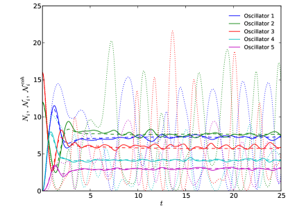
Figure 3: Quantum evolution (solid lines) and classical evolution (dotted) of the occupation numbers for the initial state (0,12,16,0,0). The dashed lines show the quantum evolution of the corresponding coherent state.

We thank Edward Witten, Charles Thorn, Joerg Jaeckel, Adam Christopherson, Gaoli Chen, Sankha Chakrabarty and Yaqi Han for useful discussions, and Mark Hertzberg for pointing out an error in our original version of this paper MH . This work was supported in part by the U.S. Department of Energy under grant No. DE-FG02-97ER41029, and by the Heising-Simons Foundation under grant No. 2015-109.

References

- (1) J. Preskill, M. Wise and F. Wilczek, Phys. Lett. B120 (1983) 127; L. Abbott and P. Sikivie, Phys. Lett. B120 (1983) 133; M. Dine and W. Fischler, Phys. Lett. B120 (1983) 137.
- (2) P. Sikivie and Q. Yang, Phys. Rev. Lett. 103 (2009) 111301.
- (3) O. Erken, P. Sikivie, H. Tam and Q. Yang, Phys. Rev. D85 (2012).
- (4) K. Saikawa and M. Yamaguchi, Phys. Rev. D87 (2013) 085010.
- (5) J. Berges and J. Jaeckel, Phys. Rev. D91 (2015) 025020.
- (6) A. Guth, M. Hertzberg and C. Prescod-Weinstein, Phys. Rev. D92 (2015) 103513.
- (7) E. Braaten, A. Mohapatra and H. Zhang, arXiv:1512.00108.
- (8) S.-J. Sin, Phys. Rev. D50 (1994) 3650; J. Goodman, New Astronomy Reviews 5 (2000) 103; W. Hu, R. Barkana and A. Gruzinov, Phys. Rev. Lett. 85 (2000) 1158; E.W. Mielke and J.A. Vélez Pérez, Phys. Lett. B671 (2009) 174; J.-W. Lee and S. Lim, JCAP 1001 (2010) 007; A. Lundgren et al., Ap. J. 715 (2010) L35; D.J. Marsh and P.G. Ferreira, Phys. Rev. D82 (2010) 103528; T. Harko, Phys. Rev. D83 (2011) 123515; P.-H. Chavanis, Astron. Astrophys. 537 (2012) A127; P. Arias et al., JCAP 1206 (2012) 013; V. Lora et al., JCAP 02 (2012) 011; T. Rindler-Daller and P. Shapiro, MNRAS 422 (2012) 135; D.J. Marsh and J. Silk, MNRAS 437 (2014) 2652; H.-Y. Schive et al., Phys. Rev. Lett. 113 (2014) 261302; B. Bozek, D.J. Marsh, J. Silk and R. Wyse, MNRAS 450 (2015) 209; E. Calabrese and D.N. Spergel, arXiv:1603.07321. P.-H. Chavanis, arXiv:1604.05904.
- (9) P. Sikivie, Phys. Lett. B695 (2011) 22.
- (10) L. Duffy and P. Sikivie, Phys. Rev. D78 (2008) 063508.
- (11) N. Banik, A. Christopherson, P. Sikivie and E. Todarello, Phys. Rev. D91 (2015) 123540.
- (12) E. Fermi, J. Pasta and S. Ulam, Los Alamos National Laboratory Report No. LA-1940, 1955; G.P. Berman and F.M. Israelev, Chaos 15 (2001) 015104.
- (13) P. Sikivie, Phys. Rev. Lett. 48 (1982) 1156.
- (14) A. Vilenkin and A.E. Everett, Phys. Rev. Lett. 48 (1982) 1867.
- (15) I.I. Tkachev, Phys. Lett. B261 (1991) 289.
- (16) S. Davidson and T. Schwetz, Phys. Rev. D93 (2016) 123509.
- (17) M. Hertzberg, arXiv:1609.01342.