Abstract

The interval Distance Geometry Problem (i DGP) consists in finding a realization in $\mathbb{R}^{K}$ of a simple undirected graph $G=(V,E)$ with nonnegative intervals assigned to the edges in such a way that, for each edge, the Euclidean distance between the realization of the adjacent vertices is within the edge interval bounds. In this paper, we focus on the application to the conformation of proteins in space, which is a basic step in determining protein function: given interval estimations of some of the inter-atomic distances, find their shape. Among different families of methods for accomplishing this task, we look at mathematical programming based methods, which are well suited for dealing with intervals. The basic question we want to answer is: what is the best such method for the problem? The most meaningful error measure for evaluating solution quality is the coordinate root mean square deviation. We first introduce a new error measure which addresses a particular feature of protein backbones, i.e. many partial reflections also yield acceptable backbones. We then present a set of new and existing quadratic and semidefinite programming formulations of this problem, and a set of new and existing methods for solving these formulations. Finally, we perform a computational evaluation of all the feasible solver$+$formulation combinations according to new and existing error measures, finding that the best methodology is a new heuristic method based on multiplicative weights updates.
Keywords: distance geometry, protein conformation, mathematical programming.

1 Introduction

The Distance Geometry Problem (DGP) is defined formally as follows: given an integer $K>0$, a simple undirected graph $G=(V,E)$, and an edge weight function $U:E\to\mathbb{R}_{+}$, establish or deny the existence of a vertex realization function $x:V\to\mathbb{R}^{K}$ such that:

$$\forall\{u,v\}\in E\qquad\|x_{u}-x_{v}\|_{2}=U_{uv};$$ (1)

realizations satisfying (1) are called valid realizations. The DGP arises in many important applications: determination of protein conformation from distance data [44], localization of mobile sensors in communication networks [21], synchronization of clocks from phase information [52], control of unmanned submarine fleets [6], spatial logic [22], and more [36]. It is NP-complete when $K=1$ and NP-hard for larger values of $K$ [51]. Notationwise, we let $n=|V|$ and $m=|E|$.

The aim of this paper is to find the quality-wise best and pratically fastest method for solving a DGP variant arising in finding the shape of proteins using incomplete and imprecise distance data. We achieve this through an extensive computational benchmark of many (new and existing) heuristic methods and many instances constructed from Protein Data Bank (PDB) data [11]. First, however, we make a theoretical contribution related to a new solution quality measure which is specially suited to evaluate the solution quality of protein isomers (i.e. proteins which have the same chemical composition but a different shape). This is necessary to evaluating the computationally obtained solutions, since the symmetry group of protein backbones contains partial reflections [37] (these are visible in most molecules, which may occur in nature in their left handed or right handed conformation).

1.1 The number of solutions

Let $\tilde{X}$ be the set of valid realizations of $G$. If $x\in\tilde{X}$, any congruence (translation, rotation, reflection) of $x$ yields another valid realization of $G$. We therefore focus on the quotient set $X=\tilde{X}/\!\sim$, where $x\sim y$ whenever there is a congruence mapping $x$ to $y$.

We have that $X=\varnothing$ if the corresponding DGP instance has no solutions; $G$ is rigid if $|X|$ is finite; $G$ is globally rigid if $|X|=1$; and $G$ is flexible if $|X|$ is uncountable. We note that $|X|$ cannot be countably infinite. By Milnor’s theorem on the Betti numbers of real algebraic varieties [46], the number of connected components of $X$ is bounded above by $2\times 3^{{nK}-1}$. Suppose that $|X|$ is countably infinite: then it cannot be flexible. This implies that incongruent elements of $X$ are on distinct connected components of the manifold containing $X$. Milnor’s theorem shows that there are only finitely many such connected components, which implies that $|X|$ is finite. This result also follows by the cylindrical decomposition theorem of semi-algebraic sets [7, 10].

1.2 Proteins and the Branch-and-Prune algorithm

Our motivating application is finding the shape of protein proteins in space (thus we fix $K=3$) knowing interval estimations of some of the inter-atomic distances [16]. The protein backbone graph $G$ belongs to a specific subclass of Henneberg type I graphs [53], namely there is an order $<$ on $V$ such that, for each $v>3$, $v$ is adjacent to $v-1,v-2,v-3$ [29]. The backbone itself provides such an order on the atoms, although other orders, which may be more convenient to algorithmic efficiency, have been defined [28, 17]. DGP instances with this property form a problem called Discretizable Molecular Distance Geometry Problem (DMDGP), which is also NP-hard [29]. In [35], we proposed a fast and accurate mixed-combinatorial algorithm for solving the DMDGP, called Branch-and-Prune (BP). Unsurprisingly, the BP has exponential complexity in the worst case, but the DMDGP has many interesting properties which hold almost surely:

• $G$ is rigid, so $|X|$ is finite; [35]

• in particular, $|X|$ is a power of two; [39]

• the BP algorithm is Fixed-Parameter Tractable (FPT) on the DMDGP [37], and in all the protein instances we tested, the parameter was always fixed at the same constant, yielding polytime behaviour.

By “almost surely” we mean that the set of weighted input graphs for which the above properties may not hold has Lebesgue measure zero in the set of all weighted input graphs (assuming the weights to be real numbers). The BP algorithm relies on the given distances being precise; unfortunately, however, inter-atomic distance data measured through Nuclear Magnetic Resonance (NMR) are subject to experimental errors, modelled as real intervals $[L,U]$ assigned to all edges $\{u,v\}$ whenever $v-u\geq 3$ in the vertex order. To overcome this difficulty, two research directions have been pursued: (i) the discretization of the uncertainty intervals [30]; (ii) the analytical description, using Clifford algebra, of the locus of vertex $v$ when the edge $\{v,v-3\}$ is weighted by an interval [27]. The formulation study in this paper moves a first step towards a third direction: the integration of purely continuous techniques within mixed-combinatorial algorithms such as BP. To this end, in this paper we pursue a computational study of some these techniques.

1.3 The interval DGP

This brings us to the interval Distance Geometry Problem (i DGP), which is a variant of the DGP defined as follows: the edge function is an interval function $[L,U]:E\to\mathbb{IR}_{+}$, where $L,U$ are two nonnegative functions from $E\to\mathbb{R}_{+}$ such that $L_{uv}\leq U_{uv}$ for each $\{u,v\}\in E$, $\mathbb{IR}_{+}$ is the set of nonnegative real intervals, and Eq. (1) is replaced by:

$$\forall\{u,v\}\in E\qquad L_{uv}\leq\|x_{u}-x_{v}\|_{2}\leq U_{uv}.$$ (2)

Note that Eq. (2) is often written as:

$$\forall\{u,v\}\in E\qquad L_{uv}^{2}\leq\|x_{u}-x_{v}\|_{2}^{2}\leq U^{2}_{uv}.$$ (3)

As explained later, Eq. (3) minimizes the chances that numerical solvers, which rely on the floating-point representation of real numbers, might stumble upon a negative representation of zero, thereby raising a “not a number” (NaN) error upon calculating the square root. Note that the i DGP contains (and hence generalizes) the DGP, since the latter corresponds to the case $L=U$.

1.4 Aim of this paper

Most solution techniques for solving i DGP instances require a continuous search in Euclidean space, even if the given graph is rigid. The most direct approach is to formulate the i DGP as a Mathematical Program (MP), which can then be solved by a MP solver. The aim of this paper is to determine the best solver$+$formulation combination for the i DGP. To this end, we need to know: (a) how to evaluate the quality of the solutions computed by the solvers; (b) which formulations to employ; (c) which solvers to employ. We therefore introduce new and existing error measures, formulations and solvers, before proceeding to evaluate them all computationally. Since we want our algorithms to be fast and scale well, we focus on heuristic approaches. This means that we forsake a proof of exactness, so evaluating these algorithms require test sets with given (trusted) solutions. Such test sets can be put together using the PDB.

1.5 Solution quality evaluation

The simplest measures used for evaluation DGP solution quality are based on computing the average or maximum relative error of the realization with respect to the given distance value on the edges. The drawback of these simple edge-based measures is that even a small error might correspond (in sufficiently large proteins) to a wrong protein shape. Even worse, plotting the DGP solution versus the trusted solution usually yields nothing to the human eye, since the alignment is likely to be completely off.

A more meaningful measure is provided by Procrustes analysis [24], also called coordinate root mean square deviation (cRMSD) [43]. Informally, this is the error derived by the best alignment, via translations and rotations, of a DGP solution to the trusted solution. It provides a visual tool for a human to evaluate the error, so even when the error is non-zero the visualization helps determine whether the error is due to floating point issues or structural differences.

Unfortunately, for protein backbones there is an added difficulty: their symmetry group includes at least one partial reflection (starting from the fourth atom along the backbone), and may include many more [39, 37, 34]: in general, the partial reflection group structure is a cartesian product of cyclic groups of order two, yielding an exponential number of elements. All of these symmetric solutions are isomers. They are equivalent from the point of view of the simple, edge-based error measures, but they may have very different cRMSD values with respect to the trusted solution. Again, visualizing a trusted solution and a DGP solution from a heuristic method with a low cRMSD might yield structures which look nothing like each other.

The first contribution of this paper is the definition of a modified error measure that extends the cRMSD in that it aligns two structures in the best possible way using translations, rotations and partial reflections, and which allows us to properly evaluate the protein backbone solutions proposed by DGP heuristics. Our new measure could be described as a “cRMSD modulo isomers”.

1.6 Innovations and outcomes

To sum up, the innovations introduced in this paper are: (i) the new cRMSD modulo isomers; (ii) some new MP formulations for the iDGP; (iii) the concept of “pointwise formulation” to be used in alternating-type algorithms; (iv) an adaptation of the Multiplicative Weights Update (MWU) algorithm to the iDGP. We conclude that the MWU algorithm with its pointwise formulation is the best combination, and that the new “square factoring” MP formulation, used within either a pure MultiStart (MS) or a Variable Neighbourhood Search (VNS) heuristic, is second best.

1.7 Structure of the paper

The rest of the paper is organized as follows. In Sect. 2, we define error measures to meaningfully compare protein backbones found algorithmically with those stored in PDB files [11], and introduce a new cRMSD type measure modulo certain partial reflection isomers. In Sect. 3, we list several formulations, relaxations and variants for the i DGP, some of which are new. In Sect. 4, we propose a new algorithm for solving the i DGP: namely, an adaptation of the Multiplicative Weights Update method [4]. In Sect. 5, we discuss comparative computational results, which show that, on average, our newly proposed algorithm provides the best quality solutions.

2 Error measures for realizations of protein graphs

Since we aim at ascertaining which formulation(s) can provide the best and/or fastest bound, we need a method to benchmark quality and speed with respect to any solution algorithm. We benchmark speed by simply measuring CPU time.

Benchmarking solution quality is more complicated. In the Turing Machine (TM) model, decision problems are in NP whenever feasible instances can be certified feasible in polynomial time. Although the DGP and i DGP are NP-hard decision problems, they are not known to be in NP: feasible instances of the DGP and i DGP can in general yield realizations with irrational components, for which polynomially-sized representations are not generally available (some simple ideas have been tried in [8] but failed to prove membership of the DGP to NP). The methods employed in this paper replace irrational numbers by floating point numbers, and, as such, do not provide a valid certificate. On the other hand, this is the situation with all real number computations that need to be carry out efficiently over medium to large-scale problems. Instead, we compute feasibility errors for the floating point solutions we obtain.

2.1 The edge error

Given a realization $x^{\ast}:V\to\mathbb{R}^{K}$, we can measure the error of $x^{\ast}$ with respect to a given i DGP instance by assigning an $\ell_{2}$-norm error to each edge $\{u,v\}$ of the graph $G=(V,E)$, given by [38]:

$$\alpha_{uv}(x^{\ast})=\max\left(0,L_{uv}-\|x^{\ast}_{u}-x^{\ast}_{v}\|_{2}\right)+\max\left(0,\|x^{\ast}_{u}-x^{\ast}_{v}\|_{2}-U_{uv}\right).$$ (4)

We remark that the corresponding error for non-interval DGP instances is:

$$\beta_{uv}(x^{\ast})=\left|\|x^{\ast}_{u}-x^{\ast}_{v}\|_{2}-U_{uv}\right|.$$

Accordingly, we define the edge error as follows:

$$\eta_{uv}(x^{\ast})=\left\{\begin{array}[]{rl}\alpha_{uv}(x^{\ast})&\mbox{if the instance is {\it i}\,DGP}\\ \beta_{uv}(x^{\ast})&\mbox{if the instance is DGP.}\end{array}\right.$$

We can now define the average error associated to the instance graph $G$ and a realization $x^{\ast}$ as:

$$\Phi(x^{\ast},G)=\frac{1}{|E|}\sum_{\{u,v\}\in E}\eta_{uv}(x^{\ast}),$$ (5)

and the maximum error as:

$$\Psi(x^{\ast},G)=\max_{\{u,v\}\in E}\eta_{uv}(x^{\ast}).$$ (6)

The above are absolute edge error measures. Relative error measures also exist, where each term $L_{uv}-\|x_{u}-x_{v}\|_{2}$ is replaced by $\frac{L_{uv}-\|x_{u}-x_{v}\|_{2}}{|L_{uv}|}$ (and similary for $\|x_{u}-x_{v}\|_{2}-U_{uv}$. Whether one or the other is used depends on the application at hand, and how poorly scaled the input data $L,U$ are. In the case of proteins, bounds are generall well scaled, as they are often between $1$ and $6$Å; so absolute error measures are more appropriate.

2.2 The coordinate root mean square deviation

The edge errors go a long way in determining when a realization $x^{\ast}$ is not valid. In many applications, however, we know a priori that a problem instance should feasible. Take e.g. the reconstruction of protein conformations from inter-atomic distances: the protein certainly exists (this is also the case when localizing sensors in wireless networks: the network is being measured, so it exists). Furthermore, we might have a given (precise or approximate) realization $\bar{x}$. In this setting, we want to evaluate the error with respect to the given realization $\bar{x}$.

An obvious way to adapt the edge error to this situation is to compute the average, over edges in $E$, of an absolute $\ell_{2}$-norm distance difference:

$$\Delta(x^{\ast},\bar{x})=\frac{1}{|E|}\sum_{\{u,v\}\in E}\left|\,\|x^{\ast}_{u}-x^{\ast}_{v}\|_{2}-\|\bar{x}_{u}-\bar{x}_{v}\|_{2}\,\right|.$$ (7)

Unfortunately this approach is wrong, since different congruent realizations yield different error values, making the comparison impossible.

To this end, the cRMSD is often used instead: i.e., translate both $x^{\ast}$ and $\bar{x}$ so that their centroids $\gamma(x^{\ast})=\gamma(\bar{x})=0$, where the centroid is the vector $\gamma(x)\in\mathbb{R}^{K}$ defined as:

$$\gamma(x)=\sum_{v\leq K}x_{v},$$ (8)

and then find the congruence $\rho$ (consisting of a rotation composed with at most one reflection) such that $\|x^{\ast}-\rho(\bar{x})\|$ is minimum. Note that the norm $\|\cdot\|$ on $\mathbb{R}^{Kn}$ is induced by the $\ell_{2}$-norm in $\mathbb{R}^{K}$:

$$\|x^{\ast}-\bar{x}\|=\sum_{v\in V}\|x_{v}^{\ast}-\bar{x}_{v}\|_{2}.$$ (9)

The cRMSD between $x^{\ast}$ and $\bar{x}$ is defined as $\min_{\rho}\|x^{\ast}-\rho(\bar{x})\|$.

2.3 Distance error modulo isometries

Although the cRMSD is widely used in computational geometry, it still falls short in one of the properties of molecules, namely isomers, which are molecules having the same chemical formula but different 3D structure.

If we consider protein backbones only, their graphs $G=(V,E)$ possess a further structural property. They have an order $<$ on $V$ such that:

1. the first $K$ vertices in the order form a clique in $G$ (clique property);

2. each vertex $v>K$ is adjacent to $v-1,\ldots,v-K$ (contiguous trilateration order property).

Although protein backbones have $K=3$, we develop the theory for general $K$. DGP instances having these properties are also collectively known as ^KDMDGP, which are a subclass of Henneberg type I graphs [25]. Contiguous trilateration orders are also known as cTOP or ^KDMDGP orders [17]. The edges induced by these properties in a ^KDMDGP graph are called discretization edges, and the edges which are not discretization edges are called pruning edges.

Many mathematical aspects of the ^KDMDGP have been investigated in the past (see [39, 37, 34]). The problem itself is NP-hard. The automorphism group of $X$ generally contains a subgroup $\mathscr{G}_{P}$ consisting of partial reflections $g_{v}$, called the pruning group, such that the action of $g_{v}$ over a realization $x\in X$ is:

$$g_{v}(x)=(x_{1},\ldots,x_{v-1},R_{x}^{v}(x_{v}),\ldots,R_{x}^{v}(x_{n})),$$ (10)

where $R_{x}^{v}$ is the reflection with respect to the affine subspace spanned by $x_{v-1}$, $\ldots$, $x_{v-K}$, and where $v$ ranges over a vertex set

$$Z=V\smallsetminus(\{1,\ldots,K\}\cup\bigcup_{\{u,w\}\in E\atop u+K<w}\{u+K+1,\ldots,w\}),$$

or, in other words, $v$ must not be “covered” by any pruning edge.

2.1 Example

Consider the DGP instance with $V=\{1,2,3,4\}$,

$$E=\{\{1,2\},\{1,3\},\{2,3\},\{2,4\},\{3,4\}\}$$

consisting of two triangles on $\{1,2,3\}$ and $\{2,3,4\}$, and $K=2$. There is a partial reflection $\rho_{1}$ fixing $1,2$ and reflecting $3,4$ across the line through $1,2$, and another partial reflection $\rho_{2}$ fixing $1,2,3$ and reflecting $4$ across the line through $1,2,3$. The range of the pruning edge $\{1,4\}$ is $\{1+K+1,\ldots,4\}=\{4\}$. Therefore, if we add $\{1,4\}$ to $E$, $Z=\{3\}$, which means that the pruning group of this instance has the single generator $\rho_{1}$.

The protein backbone isomers of a valid realization $\bar{x}$ are given by the orbit $\mathscr{G}_{P}x=\{g_{v}(x)\;|\;v\in Z\}$. It turns out that all backbone isomers in $\mathscr{G}_{P}x$ are valid realizations of the given DGP instance $G$. So we might obtain a realization $x^{\ast}$ which is a valid isomer (and hence has zero edge errors), but has a large cRMSD with the given (different) isomer $\bar{x}$.

A serious issue arises when considering i DGP instances, however: if the cRMSD between $x^{\ast}$ and $\bar{x}$ is positive, is it due to the “slack” induced by the interval edge weights, or is it due to the fact that $x^{\ast}$ and $\bar{x}$ are different isomers of essentially the same backbone (a similar issue was described in [43])? This motivates us to define the following problem:

Distance Error Modulo Isometries (DEMI). Given integers $n,K$ with $n\geq K$, two $n$-point realizations $x,y\in\mathbb{R}^{Kn}$ such that the centroids $\gamma(x)=\gamma(y)=0$, and a description of a pruning group $\mathscr{G}_{P}$, find the rotation $\rho$ and a partial reflection composition $g\in\mathscr{G}_{P}$ such that $\|x-g\rho(y)\|$ is minimum.

Note that groups can be described by listing their elements, or by a set of generators (and possibly relations) which, when multiplied together up to closure, are guaranteed to generate the whole group. The latter description is usually much shorter than the former.

We let $\partial(x,y)$ be the minimum value of $\|x-g\rho(y)\|$ which solves the DEMI. We note that $\partial$ is not a semimetric (hence not even a metric), since $\partial(x,y)$ can be zero even though $x\not=y$ (just take $y$ as a partial reflection of $x$).

2.3.1 Complexity of DEMI

The computational complexity class of DEMI depends on the description of the pruning group. If it is given explicitly, by listing all the partial reflection compositions in $\mathscr{G}_{P}$, then the trivial Algorithm 1 solves the problem in polynomial time for fixed $K$. For a realization $x\in\mathbb{R}^{Kn}$ and an integer $h\leq n$, let $x[h]$ be the partial realization $(x_{i}\;|\;1\leq i\leq h)$.

1:  Find a congruence $\rho$ minimizing $\|x[K]-y[K]\|$

2:  Let $\partial(x,y)=\min\{\|x-g\rho(y)\|\;|\;g\in\mathscr{G}_{P}\}$

Algorithm 1 SolveDEMI$(x,y{\bf,\mathscr{G}_{P}})$

Step 1 takes a polynomial amount of time for fixed $K$ (an $O(n^{K-2}\log n)$ algorithm was described in [2]), but more efficient methods exist for $K=3$, see [5, 19]. Step 2 depends linearly on the order of the pruning group, which was shown in [34] to be $2^{|Z|}$. Since $Z$ is usually small in practice (see Sect. 2.3.2) and on average (see Sect. 2.3.3), assuming the input to DEMI to be the explicit list of all partial reflection compositions is not out of place.

We have not been able to prove that DEMI can be solved in polynomial time (for fixed $K$) if its input is $x$, $n$, and the compact group generators description $Z$, nor that DEMI is NP-hard under the same conditions. We leave this as an open question.

2.3.2 Empirical observations on the size of $Z$

In this section we exhibit empirical evidence to the effect that $|Z|$ is rarely large. First, we note that $|Z|\geq 1$: this follows by the definition of $Z=\{v>K\;|\nexists\{u,w\}\in E\;(u+K<v\leq w)\}$, since $v=K+1$ is obviously always in $Z$ (this can also be shown by other means [29, Sect. 2.1]).

Figures 1-2 show the mean and standard deviations of $|Z|$ relative to samples of 500 randomly generated ^KDMDGP instances for each value of $K\in\{2,3\}$ and various values of the edge sparsity $s$. The generation procedure is as follows: given $n=|V|$ and $K$, we initially generate a ^KDMDGP instance with all the necessary discretization edges in its edge set $E$ (there are $K(K-1)/2+(n-K)K$ of them), but no pruning edges. Then we loop over all $\{i,j\}$ which are not discretization edges, and with given probability $s$ we insert a pruning edge in $E$. So $s$ is in fact the density of the pruning edges.

$s/K$	$2$	$3$
$0.1$
$0.2$
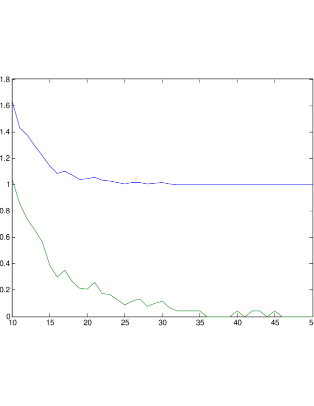
$0.3$

Figure 1: In each picture: mean (top curve) and standard deviation (bottom curve) of the pruning group size as a function of $n$ for fixed values of $K=2$ (left column), $K=3$ (right column), and the edge sparsity $s$ (values in $\{0.1,0.2,0.3\}$ in top, middle and bottom rows).

The exact dependency of $|Z|$ on the number of pruning edges is given in [37], and it is used to show that the BP algorithm is FPT. It should be clear by definition that the denser the graph, the smaller $Z$ must be. Figures 1-2 show (empirically) that $|Z|$ tends to 1 very fast and very reliably as $n$ and $s$ increase, with $n,s$ as small as, respectively, $20$ and $0.3$. Large graphs with $|Z|>1$ are very rare.

$n/K$	$2$	$3$
$10$
$15$
$20$

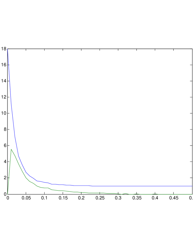
Figure 2: In each picture: mean (top curve) and standard deviation (bottom curve) of the pruning group size as a function of the edge sparsity $s$ for fixed values of $K=2$ (left column), $K=3$ (right column), and $n$ (values in $\{10,15,20\}$ in top, middle and bottom rows).

It is interesting to note that the standard deviation of $|Z|$ as a function of the sparsity $s$ has a maximum in $[0,0.05]$ (see Fig. 2). This phenomenon is analyzed below in more detail.

2.3.3 Expectation and variance of $|Z|$

As explained in Sect. 2.3, ^KDMDGP instances consist of a backbone subgraph (a minimal graph satisfying the clique and contiguous trilateration order properties) and some pruning edges. Accordingly, random ^KDMDGP graphs $G=(V,E)$ are generated as follows:

• a backbone which only depends on $K,n$ and determines the order on $V$;

• for each pair $\{u,w\}$ which is not a discretization edge, we independently add $\{u,w\}$ as a pruning edge in $E$ with probability $s\in[0,1]$.

Now consider the subset $Z\subseteq V$, defined as in Sect. 2.3 as

$$Z=\{v>K\,|\,\nexists\{u,w\}\in E\;(u+K<v\leq w)\}.$$

We consider $|Z|$ as a random variable depending on the edge probability $s$ (also known as the sparsity of the ^KDMDGP graph $G$), and compute its expected value. In the following, $\mbox{\sf P}(\cdot)$ is the probability of an event, $\mbox{\sf E}(\cdot)$ is the expectation of a random variable and $\mbox{\sf Var}(\cdot)$ is its variance.

2.2 Proposition

$\mbox{\sf E}(|Z|)\leq 1+(n-K-1)(1-s)^{n-K-1}$.

Proof.

For all $v\in\{K+1,\ldots,n\}$ define $\mathcal{X}_{v}=0$ if $v\notin Z$ and $1$ if $v\in Z$. Then $|Z|=\sum\limits_{v=K+1}^{n}\mathcal{X}_{v}$, which implies:

$$\mbox{\sf E}(|Z|)=\sum\limits_{v=K+1}^{n}\mbox{\sf E}(\mathcal{X}_{v})=\sum_{v=K+1}^{n}\mbox{\sf P}(v\in Z).$$

Now, for any $v\in\{K+1,\ldots,n\}$ there are $v-K-1$ choices of $u$ with $u+K<v$, and there are $n-v+1$ choices of $w$ with $v\leq w$. Therefore, there are $(v-K-1)(n-v+1)$ possible choices of the pruning edge $\{u,w\}$ such that $u+K<v\leq w$. Moreover, $v\in Z$ if all these pairs are not added to the graph. Thus,

$$\mbox{\sf P}(v\in Z)=(1-s)^{(v-K-1)(n-v+1)},$$

and hence:

$$\mbox{\sf E}(|Z|)=\sum_{v=K+1}^{n}(1-s)^{(v-K-1)(n-v+1)}.$$

Finally, we remark that (a) the first term of the sum is 1, and (b) $(1-s)<1$, so we can replace all the terms of the sum by the second largest one, and obtain:

$$\mbox{\sf E}(|Z|)\leq 1+(n-K-1)(1-s)^{n-K-1},$$ (11)

as claimed. ∎∎

The RHS of Eq. (11) converges to 1 as $s\to 1$ with $n,K$ fixed, and as $n\to\infty$ with $s,K$ fixed, which is consistent with the empirical results of Sect. 2.3.2. We are therefore justified in making the qualitative statements that, for random DMGDP, $|Z|\approx 1$.

We now discuss the variance. Since $\mbox{Var}(|Z|)=\mbox{Var}(\sum_{v=K+1}^{n}\mathcal{X}_{v})$, then by a property of sum of correlated variables [55], we have:

$$\mbox{Var}(|Z|) =\sum_{v=K+1}^{n}\mbox{Var}(\mathcal{X}_{v})+2\sum_{k+1\leq v_{1}<v_{2}\leq n}\mbox{Cov}(\mathcal{X}_{v_{1}},\mathcal{X}_{v_{2}})$$

$$=\sum_{v=K+2}^{n}\mbox{Var}(\mathcal{X}_{v})+2\sum_{k+2\leq v_{1}<v_{2}\leq n}\mbox{Cov}(\mathcal{X}_{v_{1}},\mathcal{X}_{v_{2}})$$

(this follows from $$\mbox{E}(\mathcal{X}_{K+1})=1 \mbox{E}(\mathcal{X}_{K+1}\mathcal{X}_{v})=\mbox{E}(\mathcal{X}_{v}) v$$ and for all )

$$=\sum_{v=K+2}^{n}\mbox{E}(\mathcal{X}_{v})+\sum_{k+2\leq v_{1}<v_{2}\leq n}\mbox{E}(\mathcal{X}_{v_{1}}\mathcal{X}_{v_{2}})+$$

$$-\sum_{v=K+2}^{n}[\mbox{E}(\mathcal{X}_{v})]^{2}-2\sum_{k+2\leq v_{1}<v_{2}\leq n}\mbox{E}(\mathcal{X}_{v_{1}})\mbox{E}(\mathcal{X}_{v_{2}}).$$

By definition of $Z$, two vertices $v_{1}$ and $v_{2}$ are in $Z$ if all pairs $\{u,w\}$ such that either $u+K<v_{1}\leq w$ or $u+K<v_{2}\leq w$ are not edges of $G$. Assume $v_{1}<v_{2}$, then there are:

$$(v_{1}-K-1)(n-v_{1}+1)+(v_{2}-K-1)(n-v_{2}+1)-(v_{1}-K-1)(n-v_{2}+1)$$

$$=\ (v_{1}-K-1)(n-v_{1}+1)+(v_{2}-v_{1})(n-v_{2}+1)$$

such edges (by counting all pairs of each type and subtracting the number of doubly counted ones). So, the probability that $v_{1},v_{2}\in Z$ is

$$(1-s)^{(v_{1}-K-1)(n-v_{1}+1)+(v_{2}-v_{1})(n-v_{2}+1)}.$$

This implies

$$\mbox{\sf Var}(|Z|) =\sum_{v=K+2}^{n}(1-s)^{(v-K-1)(n-v+1)}-\sum_{v=K+2}^{n}(1-s)^{2(v-K-1)(n-v+1)}+$$

$$\quad+2\sum_{K+2\leq v_{1}<v_{2}\leq n}(1-s)^{(v_{1}-K-1)(n-v_{1}+1)+(v_{2}-v_{1})(n-v_{2}+1)}\ -$$

$$\quad-2\sum_{K+2\leq v_{1}<v_{2}\leq n}(1-s)^{(v_{1}-K-1)(n-v_{1}+1)+(v_{2}-K-1)(n-v_{2}+1)}.$$

To simplify the analysis of $\mbox{\sf Var}(|Z|)$, we provide an upper bound.

2.3 Lemma

For all $s\in(0,1)$ and $k\geq 1$, we have $\sum\limits_{i=1}^{k-1}(1-s)^{i(k-i)}<\frac{2(1-s)^{k-1}}{s}$.

Proof.

For each $1\leq i<\lfloor\frac{k}{2}\rfloor$ we have the estimate

$$(i+1)(k-i-1)=ik+k-i^{2}-2i-1=i(k-i)+k-2i-1\geq i(k-i)+1.$$ (12)

Therefore,

$$\sum_{i=1}^{k-1}(1-s)^{i(k-i)} \leq 2\;\sum_{i=1}^{\lfloor\frac{k}{2}\rfloor}(1-s)^{i(k-i)}$$

$$\leq 2((1-s)^{k-1}+(1-s)^{k}+(1-s)^{k+1}+\ldots+(1-s)^{k-2+\lfloor\frac{k}{2}\rfloor})$$

$$<2(1-s)^{k-1}\sum_{i=0}^{\infty}(1-s)^{i}$$

$$=\frac{2(1-s)^{k-1}}{s}.$$

The second inequality follows because of estimate (12). ∎∎

We can now improve the estimate for the variance (where $n,K$ only appear in the exponent):

$$0 <\mbox{\sf Var}(|Z|)$$

$$<\sum_{v_{2}=K+2}^{n}\!\!\!\!\!(1-s)^{(v_{2}-K-1)(n-v_{2}+1)}+2\!\!\!\!\!\!\!\!\sum_{K+2\leq v_{1}<v_{2}\leq n}\!\!\!\!\!\!\!\!(1-s)^{(v_{1}-K-1)(n-v_{1}+1)+(v_{2}-v_{1})(n-v_{2}+1)}$$

$$<\sum_{i=1}^{n-K-1}(1-s)^{i(n-K-i)}+2\!\!\!\!\sum_{K+2\leq v_{1}\leq n}\left((1-s)^{(v_{1}-K-1)(n-v_{1}+1)}\sum_{i=1}^{n-v_{1}}(1-s)^{i(n-v_{1}-i+1)}\right)$$

$$<\frac{2}{s}(1-s)^{(n-K-1)}+\frac{4}{s}\sum_{K+2\leq v_{1}\leq n}\big{[}(1-s)^{(v_{1}-K-1)(n-v_{1}+1)}(1-s)^{n-v_{1}}\big{]}\qquad\mbox{(Lemma \ref{lemma ZTASUA})}$$

$$=\frac{2}{s}(1-s)^{(n-K-1)}+\frac{4}{s(1-s)}\sum_{i=2}^{n-K}(1-s)^{i(n-K-i+1)}$$

$$<\frac{2}{s}(1-s)^{(n-K-1)}+\frac{4}{s(1-s)}(\frac{2}{s}-1)(1-s)^{n-K}\qquad\mbox{(Lemma \ref{lemma ZTASUA})}$$

$$=\left(\frac{8}{s^{2}}-\frac{2}{s}\right)(1-s)^{n-K-1}.$$

For example, with $s=0.2$, $n=35$, $K=2$, the estimate yields $\left(\frac{8}{s^{2}}-\frac{2}{s}\right)(1-s)^{n-K-1}=0.15$. With $s=0.3$, $n=25$, $K=2$, we get $\left(\frac{8}{s^{2}}-\frac{2}{s}\right)x(1-s)^{n-K-1}=0.03$.

Fig. 2 shows that the standard deviation (and hence the variance) of $|Z|$ has a maximum when $s$ is close to zero. Fixing $n$ and $K$, consider $\mbox{\sf Var}(|Z|)$ as a function $f(t)$ of $1-s$, let $\tau(k)=kt^{k}$, and rewrite $\mbox{\sf Var}(|Z|)$ as:

$$\mbox{\sf Var}(|Z|)=f(t) =\sum_{v=K+2}^{n}t^{(v-K-1)(n-v+1)}-\sum_{v=K+2}^{n}t^{2(v-K-1)(n-v+1)}+$$

$$\quad+2\sum_{K+2\leq v_{1}<v_{2}\leq n}t^{(v_{1}-K-1)(n-v_{1}+1)+(v_{2}-v_{1})(n-v_{2}+1)}-$$

$$\quad-2\sum_{K+2\leq v_{1}<v_{2}\leq n}t^{(v_{1}-K-1)(n-v_{1}+1)+(v_{2}-K-1)(n-v_{2}+1)}.$$

Taking the derivative of $f(t)$, we have:

$$f^{\prime}(t) =t^{-1}\left(\sum_{v=K+2}^{n}\tau((v-K-1)(n-v+1))-\sum_{v=K+2}^{n}\tau(2(v-K-1)(n-v+1))\;+\right.$$

$$\quad+2\sum_{K+2\leq v_{1}<v_{2}\leq n}\tau\big{(}(v_{1}-K-1)(n-v_{1}+1)+(v_{2}-v_{1})(n-v_{2}+1)\big{)}\;-$$

$$\left.\quad-2\sum_{K+2\leq v_{1}<v_{2}\leq n}\tau((v_{1}-K-1)(n-v_{1}+1)+(v_{2}-K-1)(n-v_{2}+1))\right).$$

Consider the derivative of $\tau$ with respect to $k$, $\tau^{\prime}(k)=(kt^{k})^{\prime}=t^{k}(1+k\ln(t))$, and take for example $k\geq 20$ and $t\leq 0.95$. We have $(1+k\ln(t))\leq 1+20\ln(0.95)=-0.026<0$. Therefore, when $t<0.95$, $\tau(k)$ is a decreasing function on the set $\{k\;|\;k\geq 20\}$. It means that, whenever $n-K-1\geq 20$, $\tau((v-K-1)(n-v+1))\geq\tau(2(v-K-1)(n-v+1))$ for each $v\in\{K+2,\ldots,n\}$, and $\tau((v_{1}-K-1)(n-v_{1}+1)+(v_{2}-v_{1})(n-v_{2}+1))\geq\tau((v_{1}-K-1)(n-v_{1}+1)+(v_{2}-K-1)(n-v_{2}+1))$ for each $v_{1}<v_{2}\in\{K+2,\ldots,n\}$, since all values under $\tau$ are at least $20$. We therefore have that $f^{\prime}(t)\geq 0$ for all $t<0.95$, i.e., whenever $s\in[0.05,1]$, $\mbox{\sf Var}(|Z|)$ decreases as $s$ increases. In other words, the maximum of $\mbox{\sf Var}(|Z|)$ can only be attained on $[0,0.05]$.

We can generalize this example to the following result.

2.4 Lemma

For fixed $n,K$, the maximum of $\mbox{\sf Var}(|Z|)$ can only be attained at $s\in[0,\frac{1}{n-K-1}]$.

Proof.

We have

$$\tau^{\prime}(k)<0\Leftrightarrow 1+k\ln(t)<0\Leftrightarrow\ln(\frac{1}{t})>\frac{1}{k}\Leftrightarrow\frac{1}{t}>e^{1/k}\Leftrightarrow t<e^{-1/k}\Leftrightarrow s>1-e^{-1/k}.$$

Since

$$e^{-1/k}=1-\frac{1}{k}+\frac{1}{2!k^{2}}-\frac{1}{3!k^{3}}+\ldots>1-\frac{1}{k},$$

we have $1-e^{-1/k}<\frac{1}{k}$. Therefore, if $s>\frac{1}{k}$ we have $\tau^{\prime}(k)<0$. So, when $s>\frac{1}{n-K-1}$, we have $\tau^{\prime}(k)<0$ for all $k\geq n-K-1$. Now the same argument as in the example above shows that $\mbox{\sf Var}(|Z|)$ decreases on the set $[\frac{1}{n-K-1},\infty)$. ∎∎

2.3.4 Computing DEMI measures in practice

We believe we made a convincing argument that we can safely use Alg. 1 to solve DEMI instances. There is, however, a glitch: none of the PDB instances we consider actually comes with a pre-defined cTOP order. For some of them, the protein backbone is a cTOP order. For others this is not the case. The state of the art in automatically finding cTOP orders in graphs is severely limited [17], and certainly does not scale to hundreds of vertices easily. Thus the DEMI measure $\partial(x,y)$ of a realization $x$ with respect to a given realization $y$ will not be computed for all instances we test in Sect. 5, but only for some (see Table 10).

3 New and existing i DGP formulations

All formulations we consider are box-constrained to bounds $x\in[M^{L},M^{U}]^{Kn}$, which have to be large enough to accommodate a worst-case realization with the given distances. One could take for example $M^{L}=-\frac{1}{2}\sum_{\{u,v\}\in E}U_{uv}$ and $M^{U}=-M^{L}$, and then tighten these bounds using some pre-processing techniques [9]. We do not write these bounds explicitly in the formulations below. Notationwise, $\mathbf{M}=[M^{L},M^{U}]^{m}$ and $\mathbf{M}^{+}=\mathbf{M}\cap[0,+\infty]$.

Most formulations come with variants. A common variant, which we refer to as the square root variant, is the following: replace $\|x_{u}-x_{v}\|_{2}^{2}$ by $\|x_{u}-x_{v}\|_{2}$ and squared distance bounds by distance bounds. In such variants, because of floating point issues, $\sqrt{\alpha}$ is implemented as $\sqrt{\alpha+\delta}$, where $\delta$ is a constant in $O(10^{-10})$.

In all of our formulations, aside from the semidefinite programming (SDP) ones, we fix the centroid at the origin, which means that we find solutions modulo translations. This seems to improve the overall reliability and convergence speed of the heuristic solution algorithms we use. It is interesting that this ceases to be the case if we also impose no rotation by fixing the first $K$ vertices, in which case the algorithms find much worse local optima.

3.1 Validation

With each formulation, we present performances and results on a single PDB instance called tiny, which describes a graph $G_{\mbox{\scriptsize\tt tiny}}=(V,E)$ with $|V|=37$, $|E|=335$ and $K=3$. Fig. 3 shows a heat map of the partial Euclidean Distance Matrix (pEDM) and the correct realization (found in the PDB file) in $\mathbb{R}^{K}$ using two types of plots.

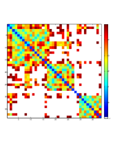
Figure 3: The tiny instance: a heat map of the pEDM (upper left) and the correct realization in $\mathbb{R}^{K}$ shown by the Jmol molecular visualization software (lower left) and in a Euclidean space plot, using the natural vertex order (right). The axes of the two 3D plots are not aligned to minimize overlap. The atom which appears disconnected in the Jmol plot corresponds to vertex 28 in the Euclidean plot, and the nine atoms in a pentagonal arrangement correspond to vertices 29-37.

These validation experiments consist in solving the tiny instance using three different Global Optimization (GO) methods. The first method is a deterministic GO solver based on spatial Branch-and-Bound (sBB) [9], which we run for at most 900s. The second method is a stochastic matheuristic called Variable Neighbourhood Search (VNS), described in [32] with some adaptations from [41]. The third method is a straightforward MultiStart (MS) algorithm, which is possibly the simplest stochastic metaheuristic, and consists of deploying a certain number of local descents from randomly sampled initial points. Both VNS and MS were allowed to run for at most 20s of user CPU time (but terminated whenever they found an optimum with average error less than $10^{-6}$). The results report the average edge error $\Phi$ (see Eq. (5)), the maximum edge error $\Psi$ (see Eq. (6)), the DEMI measure $\partial$, and the CPU time in seconds. All statistics referring to stochastic algorithms are averaged over 10 runs.

These validation experiments were conducted on a single core of a two-core Intel i7 CPU running at 2.0GHz with 8GB RAM under the Darwin Kernel v. 13.3.0. Our sBB solver of choice is Couenne [9] in its default setting. We used AMPL [23] to implement the VNS and MS algorithm, and Ipopt [18, 54] as a local solver. The SDP formulations were modelled using YalMIP [42] running under MATLAB [45] and solved using Mosek [48].

The point of these preliminary experiments is to visually show how the DEMI error measure $\partial$ impacts structural differences versus floating point errors. Each 3D plot contains two realizations (seen from the angle which best emphasizes their differences): the trusted solution found in the PDB, and the output of the corresponding algorithm. Floating point errors can be remarked when two realizations are almost aligned but not quite superimposed. Structural errors are evident when no alignment is visible.

3.2 Exact formulations

These formulations will yield a valid realization at every global optimum.

3.2.1 Penalty minimization

This formulation minimizes the sum of non-negative penalties $s_{uv}$ deriving from the fact that $\|x_{u}-x_{v}\|_{2}$ is smaller than $L_{uv}$ or larger than $U_{uv}$:

$$\left.\begin{array}[]{rrcl}\min\limits_{s\in\mathbf{M}^{+},x}&\sum\limits_{\{u,v\}\in E}s_{uv}&&\\ \forall\{u,v\}\in E&L^{2}_{uv}-\|x_{u}-x_{v}\|_{2}^{2}&\leq&s_{uv}\\ \forall\{u,v\}\in E&\|x_{u}-x_{v}\|_{2}^{2}-U^{2}_{uv}&\leq&s_{uv}\\ \forall k\leq K&\sum\limits_{v\in V}x_{vk}&=&0.\end{array}\right\}$$ (13)

Variants: (i) replace $\sum$ with $\max$; (ii) use different variables $s^{L},s^{U}$ to represent penalties w.r.t. $L,U$; (iii) replace the objective by any positive linear form in the penalty variables.

This formulation and its variants have the property that an optimum is global if and only if the objective function value is identically zero. An unconstrained and weighted version of this formulation appeared in [47]. The performance of the penalty minimization formulation and its variants on the tiny instance is shown in Table 1.

	Original			Var. (i)			Var. (ii)			Var. (iii)
Solver	$\Phi$	$\Psi$	CPU	$\Phi$	$\Psi$	CPU	$\Phi$	$\Psi$	CPU	$\Phi$	$\Psi$	CPU
Couenne	0	0	38.89	0	0	146	0	0	22.05	$\infty$	$\infty$	900
$x_{\mbox{\tiny\tt tiny}}$ and $x_{\mbox{\tiny DEMI}}$										(No solution)
$\partial$	0.3540			2.9834			0.6072			$\infty$
VNS	0	0	2.27	0.01	0.19	2.76	0.01	0.15	1.09	0	0	3.48
$x_{\mbox{\tiny\tt tiny}}$ and $x_{\mbox{\tiny DEMI}}$
$\partial$	0.4024			1.1480			1.5853			1.5464
MS	0	0	1.90	0	0	2.28	0	0	1.82	0	0	1.54
$x_{\mbox{\tiny\tt tiny}}$ and $x_{\mbox{\tiny DEMI}}$
$\partial$	0.3108			0.5983			3.6933			0.4156

Table 1: Performance of penalty minimization on tiny. For each solver and formulation (variant), we report the edge errors $\Phi,\Psi$, the CPU time, a 3D plot of the solution $x_{\mbox{\tt\scriptsize tiny}}$ given in the PDB file versus the solution $x_{\mbox{\scriptsize DEMI}}$ found by solving the DEMI instance with $x=x_{\mbox{\tt\scriptsize tiny}}$ and $y$ given by the solution of the solver, and the corresponding DEMI measure $\partial(x,y)=\min\limits_{g,\rho}\|x-g\rho(y)\|$.

3.2.2 Square factoring

This formulation has been adapted to the interval case from [20]. It exploits the identity $\|x_{u}-x_{v}\|_{2}^{2}=(x_{u}-x_{v})(x_{u}-x_{v})$:

$$\left.\begin{array}[]{rrcl}\min\limits_{x,\sigma\in\mathbf{M}^{K},\tau\in\mathbf{M}^{K}}&\sum\limits_{\{u,v\}\in E}\sum\limits_{k\leq K}(\sigma_{uvk}-\tau_{uvk})^{2}&&\\ \forall\{u,v\}\in E,k\leq K&x_{uk}-x_{vk}&=&\sigma_{uvk}\\ \forall\{u,v\}\in E&\sum\limits_{k\leq K}\sigma_{uvk}\tau_{uvk}&\geq&L_{uv}^{2}\\ \forall\{u,v\}\in E&\sum\limits_{k\leq K}\sigma_{uvk}\tau_{uvk}&\leq&U_{uv}^{2}\\ \forall k\leq K&\sum\limits_{v\in V}x_{vk}&=&0.\end{array}\right\}$$ (14)

We propose no variants for this formulation. The performance of the square factoring formulation on the tiny instance is shown in Table 2.

Solver	$\Phi$	$\Psi$	CPU
Couenne	0	0	3.11
$x_{\mbox{\tiny\tt tiny}}$ and $x_{\mbox{\tiny DEMI}}$
$\partial$	6.3182
VNS	0.01	0.02	4.05
$x_{\mbox{\tiny\tt tiny}}$ and $x_{\mbox{\tiny DEMI}}$
$\partial$	13.6406
MS	0	0	2.31
$x_{\mbox{\tiny\tt tiny}}$ and $x_{\mbox{\tiny DEMI}}$
$\partial$	0.6072

Table 2: Performance of square factoring on tiny. For each solver, we report the edge errors $\Phi,\Psi$, the CPU time, a 3D plot of the solution $x_{\mbox{\tt\scriptsize tiny}}$ given in the PDB file versus the solution $x_{\mbox{\scriptsize DEMI}}$ found by solving the DEMI instance with $x=x_{\mbox{\tt\scriptsize tiny}}$ and $y$ given by the solution of the solver, and the corresponding DEMI measure $\partial(x,y)=\min\limits_{g,\rho}\|x-g\rho(y)\|$.

3.3 Relaxations

These are formulations which relax some feasibility constraints. The obtained solution may or may not be a valid (feasible) solution to the given instance. One should always therefore verify that the solution satisfies (2). On the other hand, if a relaxation is infeasible, then so must be the original i DGP instance.

3.3.1 Convexity and concavity

This formulation, adapted to the interval case from [20], exploits the convexity and concavity of the equations in Eq. (3) separately:

$$\left.\begin{array}[]{rrcl}\max\limits_{x}&\sum\limits_{\{u,v\}\in E}\|x_{u}-x_{v}\|_{2}^{2}&&\\ \forall\{u,v\}\in E&\|x_{u}-x_{v}\|_{2}^{2}&\leq&U_{uv}^{2}\\ \forall k\leq K&\sum\limits_{v\in V}x_{vk}&=&0.\end{array}\right\}$$ (15)

Variants: replace the objective with a positively weighted version thereof.

Eq. (15) is an exact reformulation (in the sense of [31]) of

$$\min_{x}\sum\limits_{\{u,v\}\in E}(\|x_{u}-x_{v}\|^{2}-U_{uv}^{2})^{2},$$ (16)

which is possibly the best known Mathematical Programming (MP) formulation of the (non-interval) DGP so far. That Eq. (16) and Eq. (15) have the same solutions can be intuitively visualized the edges $\{u,v\}$ of the underlying graph $G$ as a set of interconnected cables, each of length $U_{uv}$: the objective of Eq. (15) “pulls” the adjacent vertices $u,v$ apart as far as possible. As a result, all cables can be straightened if and only if the DGP has a valid solution. A formal proof of this fact is given elsewhere [40].

If the given instance is an i DGP one, however, Eq. (15) is a relaxation of the lower bounding constraints: by attempting to maximize the distance between adjacent points, one hopes that $\|x_{u}-x_{v}\|_{2}\geq L_{uv}$ will hold, but this need not necessarily be the case. The performance of the convexity and concavity formulation and its variants on the tiny instance is shown in Table 3.

	Original			Var. (i)
Solver	$\Phi$	$\Psi$	CPU	$\Phi$	$\Psi$	CPU
Couenne	0	0.03	1.78	0	0.03	1.53
$x_{\mbox{\tiny\tt tiny}}$ and $x_{\mbox{\tiny DEMI}}$
$\partial$	2.0211			3.6479
VNS	0	0.33	8.80	0	0.36	8.94
$x_{\mbox{\tiny\tt tiny}}$ and $x_{\mbox{\tiny DEMI}}$
$\partial$	2.0211			2.3988
MS	0	0.33	20.19	0	0.35	20.12
$x_{\mbox{\tiny\tt tiny}}$ and $x_{\mbox{\tiny DEMI}}$
$\partial$	2.0211			2.8338

Table 3: Performance of convexity and concavity on tiny. For each solver and formulation (variant), we report the edge errors $\Phi,\Psi$, the CPU time, a 3D plot of the solution $x_{\mbox{\tt\scriptsize tiny}}$ given in the PDB file versus the solution $x_{\mbox{\scriptsize DEMI}}$ found by solving the DEMI instance with $x=x_{\mbox{\tt\scriptsize tiny}}$ and $y$ given by the solution of the solver, and the corresponding DEMI measure $\partial(x,y)=\min\limits_{g,\rho}\|x-g\rho(y)\|$.

3.3.2 Semidefinite programming relaxation

This is a natural SDP relaxation, similar to many which already appeared in the literature, where $\|x_{u}-x_{v}\|_{2}^{2}$ is linearized to $X_{uu}+X_{vv}-2X_{uv}$:

$$\left.\begin{array}[]{rrcl}\max\limits_{X\succeq 0}&\sum\limits_{\{u,v\}\in E}(X_{uu}+X_{vv}-2X_{uv})&&\\ \forall\{u,v\}\in E&X_{uu}+X_{vv}-2X_{uv}&\geq&L^{2}_{uv}\\ \forall\{u,v\}\in E&X_{uu}+X_{vv}-2X_{uv}&\leq&U^{2}_{uv},\end{array}\right\}$$ (17)

where $X\succeq 0$ means that $X$ is required to be positive semidefinite. Several SDP formulations for the DGP have been proposed in the literature over the years, see e.g. [56, 1, 13, 14]. Our formulation, which addresses the i DGP, is directly inspired by those in [12], since it employs a linearization of the constraints in Eq. (3). As objective function, we employ a linearization of $\sum_{\{u,v\}\in E}\|x_{u}-x_{v}\|^{2}$, which is unusual. We observed empirically that this yields a good performance on datasets arising from protein conformation.

Variants: replace the objective with $\min\mbox{Tr}(X)$ as a proxy to rank minimization [15]. The performance of the SDP relaxation and its variant on the tiny instance is shown in Table 4.

	Original			Var. (i)
Solver	$\Phi$	$\Psi$	CPU	$\Phi$	$\Psi$	CPU
Mosek	0.0153	0.3140	1.37	0.4704	2.4810	1.35
$x_{\mbox{\tiny\tt tiny}}$ and $x_{\mbox{\tiny DEMI}}$
$\partial$	2.3972			15.6098

Table 4: Performance of semidefinite programming on tiny. For each formulation (variant), we report the edge errors $\Phi,\Psi$, the CPU time, a 3D plot of the solution $x_{\mbox{\tt\scriptsize tiny}}$ given in the PDB file versus the solution $x_{\mbox{\scriptsize DEMI}}$ found by solving the DEMI instance with $x=x_{\mbox{\tt\scriptsize tiny}}$ and $y$ given by the solution of the solver, and the corresponding DEMI measure $\partial(x,y)=\min\limits_{g,\rho}\|x-g\rho(y)\|$.

3.3.3 Yajima’s SDP relaxation

This formulation was proposed in [56]. The term $2\sum_{\{u,v\}\in E}X_{uv}$ added to the objective function is equal to $\mbox{Tr}(\mathbf{1}X)$ (where $\mathbf{1}$ is the all-one matrix) and has a regularization purpose, ensuring that $\mbox{Tr}(\mathbf{1}X)=0$ and hence that $\mbox{rk}(X)\leq n-1$.

$$\left.\begin{array}[]{rrcl}\min\limits_{s\in\mathbf{M}^{+},X\succeq 0}&\sum\limits_{\{u,v\}\in E}(s_{uv}-(X_{uu}+X_{vv}-2X_{uv})+L^{2}_{uv})&+&2\sum\limits_{\{u,v\}\in E}X_{uv}\\ \forall\{u,v\}\in E&(X_{uu}+X_{vv}-2X_{uv})-L^{2}_{uv}&\leq&s_{uv}\\ \forall\{u,v\}\in E&2(X_{uu}+X_{vv}-2X_{uv})-L^{2}_{uv}-U^{2}_{uv}&\leq&s_{uv}\end{array}\right\}$$ (18)

We propose no variants for this formulation. The performance of Yajima’s SDP relaxation on the tiny instance is shown in Table 5.

	Original
Solver	$\Phi$	$\Psi$	CPU
Mosek	0.3864	2.6086	1.65
$x_{\mbox{\tiny\tt tiny}}$ and $x_{\mbox{\tiny DEMI}}$
$\partial$	27.3586

Table 5: Performance of Yajima’s SDP on tiny. We report the edge errors $\Phi,\Psi$, the CPU time, a 3D plot of the solution $x_{\mbox{\tt\scriptsize tiny}}$ given in the PDB file versus the solution $x_{\mbox{\scriptsize DEMI}}$ found by solving the DEMI instance with $x=x_{\mbox{\tt\scriptsize tiny}}$ and $y$ given by the solution of the solver, and the corresponding DEMI error $\partial(x,y)=\min\limits_{g,\rho}\|x-g\rho(y)\|$.

3.4 A pointwise reformulation

Pointwise reformulations are only exact for a specific set of values assigned to certain parameters. Typically, replacing variables or entire terms by parameters makes it possible to obtain formulations for which there exist very efficient solution methods. This reformulation will be used in a stochastic search setting (see Sect. 4 below) where the global search phase occurs over the parameter values.

We replace the term $(x_{uk}-x_{vk})^{2}=(x_{uk}-x_{vk})(x_{uk}-x_{vk})$ by a linear term $\theta_{uvk}(x_{uk}-x_{vk})$ whenever it occurs in Eq. (3) and (15) in a nonconvex way:

$$\left.\begin{array}[]{rrcl}\max\limits_{x}&\sum\limits_{\{u,v\}\in E}\sum\limits_{k\leq K}\theta_{uvk}(x_{uk}-x_{vk})&&\\ \forall\{u,v\}\in E&\|x_{u}-x_{v}\|_{2}^{2}&\leq&U_{uv}^{2}\\ \forall\{u,v\}\in E&\sum\limits_{k\leq K}\theta_{uvk}(x_{uk}-x_{vk})&\geq&L_{uv}^{2}.\end{array}\right\}$$ (19)

It should be clear that for each solution $x^{\ast}$ of Eq. (3), there is a parameter matrix $\theta^{\ast}\in\mathbb{R}^{mK}$ such that $x^{\ast}$ is a feasible solution of Eq. (19): it suffices to choose $\theta_{uvk}^{\ast}=(x^{\ast}_{uk}-x^{\ast}_{vk})$ for each $\{u,v\}\in E$ and $k\leq K$. Note that Eq. (19) is a convex MP, and can therefore be solved efficiently. We let $\mbox{\sf PtwCvx}(\theta)$ be the solution of Eq. (19) with input parameters $\theta$.

4 A new i DGP algorithm

In this section we discuss an adaptation to the i DGP of the well-known MWU method [4]. As explained in [4], the MWU is in fact a meta-algorithm: it has been rediscovered along the years applied to many different optimization problems. Differently from most meta-heuristics, the MWU is as much a theoretical tool as a practical method, insofar as it provides a “generic” asymptotic performance guarantee which works for all problems where the MWU applies. The performance guarantee proof can be modified according to the specific features of the given problem to yield theoretical results. Among the problems listed in [4], possibly the most interesting for the GO community are the Plotkin-Shmoys-Tardos LP feasibility approximation algorithm [50] and the SDP approximation algorithm in [3].

The MWU is applied to a multi-iteration setting over a given horizon $\{1,\ldots,T\}$ where, at each iteration $t\leq T$, $m$ “advisors” express an opinion about a certain decision. The advisors’ opinion yield a gain/loss vector $\psi^{t}=(\psi^{t}_{i}\;|\;i\leq m)$ in $[-1,1]^{m}$. The MWU method associates a discrete distribution $\rho^{t}=(\rho^{t}_{i}\;|\;i\leq m)$ on the advisors, which is updated using the rule

$$\omega^{t}_{i}=\omega^{t-1}_{i}(1-\eta\psi_{i}^{t-1})$$ (20)

for each $t>1$, where $\rho^{t}_{i}=\frac{\omega^{t}_{i}}{\sum_{\ell}\omega^{t}_{i}}$ and $\eta\leq\frac{1}{2}$ is a user-defined parameter. This distribution essentially measures the reliability of each advisor. The method then stochastically takes the decision given by advisor $i$ with probability $\rho^{t}_{i}$. The average gain/loss made by MWU is therefore given by the weighted average $\Omega^{t}=\psi^{t}\cdot\rho^{t}$. It is shown in [4] that the following bound holds:

$$\sum_{t\leq T}\Omega^{t}\leq\sum_{t\leq T}\psi_{\ell}^{t}+\eta\sum_{t\leq T}|\psi_{\ell}^{t}|+\frac{\ln m}{\eta},$$ (21)

where $\ell$ is the index of the best advisor on average over all iterations. For fixed $m$ and $T\to\infty$, Eq. (21) states that the cumulative gain/loss made by the MWU method is bounded by a (piecewise) linear function of the gain/loss made by the best advisor, which is somewhat counterintuitive, given that $\ell$ is not known in advance.

4.1 The MWU method in the i DGP setting

We now reinterpret the MWU method in the setting of the i DGP, which aims to solve the problem via the pointwise reformulation Eq. (19). Consider a loop over $T$ iterations: the convex pointwise reformulation Eq. (19) is solved at each iteration and efficiently yields a candidate realization $\bar{x}$. This is then refined using $\bar{x}$ as a starting point to a local Nonlinear Programming (NLP) solver applied to the penalty minimization formulation of Eq. (13), which yields a current iterate $x$.

We now explain how $x$ is used to stochastically update $\theta$ at iteration $t\leq T$ along the lines of the MWU method (see the summary in Fig. 4):

• let $(D_{uv})=(\|x_{u}-x_{v}\|\;|\;u,v\in V)$ be the distance matrix corresponding to $x$;

• for each $\{u,v\}\in E$ and $t\leq T$, let:

  $$\psi_{uv}^{t}=\frac{\alpha_{uv}}{\max\limits_{\{w,z\}\in E}\alpha_{wz}}$$ (22)

  be the relative error of $D$ with respect to $[L,U]$, where $\alpha_{uv}$ is defined in Eq. (4) — note that $\psi^{t}$ is a scaled edge error vector with every component in $[0,1]$;

• for each $\{u,v\}\in E$ and $1<t\leq T$ let

  $$\omega_{uv}^{t}=\omega_{uv}^{t-1}(1-\eta\psi_{uv}^{t-1});$$ (23)

  Figure 4: The update of $\theta$ from a candidate realization $x$ at each iteration $t$ of the MWU method. The oracle $\mbox{\sf PtwCvx}(\theta)$ solves the pointwise reformulation Eq. (19) parametriezd with $\theta$, and uses the solution as a starting point to a local NLP algorithm solving an exact formulation of the i DGP, say Eq. (13).

• let $\theta_{uvk}$ be a random value sampled from the uniform distribution on $[0,\omega_{uv}(x_{uk}-x_{vk})]$.

We remark that the distribution $\rho^{t}$ is defined in terms of the edge weights $\omega^{t}$:

$$\rho_{uv}^{t}=\frac{\omega_{uv}^{t}}{\sum\limits_{\{w,z\}\in E}\omega_{wz}^{t}}.$$ (24)

The MWU method applied to the i DGP is given as Alg. 2.

1:  let $\omega^{0}=1$

2:  let $x$ be the output of a local NLP solver applied to Eq. (13)

3:  let $x^{\prime}=x$ be the best solution so far

4:  for $t\leq T$ do

5:     derive $\theta$ from $x$ as explained above

6:     compute a new candidate realization $\bar{x}=\mbox{\sf PtwCvx}(\theta)$

7:     let $x$ be the solution returned by a local NLP solver on Eq. (13) with $\bar{x}$ as starting point

8:     if $x$ is an improvement with respect to $x^{\prime}$ according to the average error $\Omega^{t}$, let $x=x^{\prime}$

9:  end for

Algorithm 2 $\mbox{\sc MultiplicativeWeightsUpdate}(\eta,T)$

4.2 The MWU approximation guarantee for the i DGP

One specific feature of the i DGP is that the “advisors” never yield gains but only a cost vector $\psi^{t}$ having components in $[0,1]$. This allows us to prove the following result:

4.1 Proposition

After $T$ iterations of the MWU method, the following relationship holds:

$$\min_{t\leq T}\Omega^{t}\leq\frac{1}{T}\left(\frac{\ln m}{\eta}+(1+\eta)\min_{\{u,v\}\in E}\sum_{t\leq T}\psi_{uv}^{t}\right).$$ (25)

Proof.

By Line 8 in Alg. 2, $\min\limits_{t\leq T}\Omega^{t}$ is the per-edge error (weighted by the distribution $p^{t}$) associated to $x^{\prime}$. From Eq. (21), because $\psi_{uv}^{t}\geq 0$ for all $\{u,v\}\in E,t\leq T$, we get $\psi_{uv}^{t}=|\psi_{uv}^{t}|$, whence, by definition of $\ell$ in Eq. (21):

$$\sum_{t\leq T}\Omega^{t}\leq(1+\eta)\min_{\{u,v\}\in E}\sum_{t\leq T}\psi_{uv}^{t}+\frac{\ln m}{\eta}.$$

Since $x^{\prime}$ is the realization with lowest error over all $t\leq T$, then $T\min\limits_{t\leq T}\Omega^{t}\leq\sum\limits_{t\leq T}\Omega^{t}$, which implies:

$$T\min_{t\leq T}\Omega^{t}\leq(1+\eta)\min_{\{u,v\}\in E}\sum_{t\leq T}\psi_{uv}^{t}+\frac{\ln m}{\eta}.$$

Dividing through by $T$ yields the result. ∎∎

We remark that the RHS of Eq. (21) is the average weighted error of the best realization found by the MWU in $T$ iterations. Prop. 25 states that this error is in the order of a linear function of the smallest scaled error (see Eq. (22)) over all edges.

4.3 Pointwise reformulation feasibility

Although the pointwise reformulation is exact for a certain value of $\theta$, it may fail to even be feasible for certain other values of $\theta$. Since this would be an issue for the MWU method, we further relax it to the following (always feasible) form:

$$\left.\begin{array}[]{rrcl}\max\limits_{x,s}&\sum\limits_{\{u,v\}\in E}\left(\sum\limits_{k\leq K}\theta_{uvk}(x_{uk}-x_{vk})-s_{uv}\right)&&\\ \forall\{u,v\}\in E&\|x_{u}-x_{v}\|_{2}^{2}&\leq&U_{uv}^{2}\\ \forall\{u,v\}\in E&\sum\limits_{k\leq K}\theta_{uvk}(x_{uk}-x_{vk})&\geq&L_{uv}^{2}-s_{uv}\\ &s&\geq&0.\end{array}\right\}$$ (26)

5 Computational assessment

The aim of this section is to present results obtained by four solvers (MS, VNS, MWU, and Mosek) over 19 different formulations, for each of 61 i DGP instances. Since not every solver can be applied to every formulation, and sometimes errors are generated for combinations of solver$+$formulation with some of the instances, the number of measure vectors is less than $4\times 19\times 61$.

5.1 Solver$+$formulation combinations

More precisely, we apply MS and VNS to Eq. (13) and its 4 variants (the square root variant and 3 explicitly listed ones), Eq. (14) and its square root variant, Eq. (15) and its positively weighted objective function variant, for a total of 9 formulations. We apply MWU to Eq. (19), and Mosek to Eq. (17) and its trace variant, and to Eq. (18). We therefore consider 22 different solver$+$formulation combinations.

Unlike in the validation experiments, we did not consider the sBB solver as most instances are excessively difficult. The rest of the solver set-up is the same. The solvers MS, VNS, MWU, which are all implemented in AMPL, solve NLP subproblems at each iteration using the local NLP solver Ipopt. The SDP formulations were modelled using YalMIP running under MATLAB and solved using Mosek. Like the validation experiments, all results were obtained on an Intel i7 CPU running at 2.0GHz with 8GB RAM under the Darwin Kernel v. 13.3.0.

5.2 User-configurable parameters

Each of the MP solvers was given at most 20s of user CPU time, excluding the time taken by Ipopt. Each call to Ipopt was also limited to 20s; however, the Ipopt documentation warns that its stopwatch is not checked regularly, but only after certain operations, which on certain instances appear to take place very rarely. This is apparent in Table 9, where many solvers exceed the 20s CPU time limit. Mosek was given no time limit, since we wanted to find the optimal solution of the SDP.

All tolerances in the AMPL code were set to $1\times 10^{-6}$. Ipopt was used in its default configuration. The VNS maximum neighbourhood radius and the maximum number of local searches deployed in each neighbourhood were both set to $5$. The $\eta$ parameter in MWU was set to $0.5$ (its maximum value) after some preliminary testing. Mosek was used in its default configuration.

5.3 Instances

Instances were obtained from a selection of PDB files by extracting all the atomic coordinates, computing all of the inter-atomic distances, and discarding all those distances exceeding $5$Å (so as to mimic NMR data). More precisely, covalent bonds and angles are known fairly precisely; since each covalent angle is incident to two covalent bonds, the remaining side of the triangle they define can also be computed precisely. Other known distances can be found through NMR experiments, which yield an interval measurement. We extracted the protein backbone from each considered PDB dataset, computed all precise distances, and then we replace all other distances $d_{uv}$ smaller than $5$Å by the interval $[d_{uv}-0.1d_{uv},d_{uv}+0.1d_{uv}]$.

The mean pruning group generator size $|Z|$ over the test instances is 1.78 and the standard deviation is 4.92, but this is due to a single outlier with $|Z|=34$. Removing the outlier, we have mean $|Z|$ 1.04 and standard deviation 0.30, consistent with Sect. 2.3.2. The sparsity of the pruning edges over the test instances is 0.14.

Table 6 reports the instance names, their sizes, and whether they are classified as easy or hard (last column), see Sect. 5.5.

Instance	$|V|$	$|E|$	Hard?
100d	489	5741	H
1guu-1	150	959	H
1guu-4000	150	968	H
1guu	150	955	H
1PPT	302	3102	H
2erl-frag-bp1	39	406
2kxa	177	2711	H
C0020pdb	107	999	H
C0030pkl	198	3247	H
C0080create.1	60	681	H
C0080create.2	60	681	H
C0150alter.1	37	335	H∗
C0700odd.1	18	39
C0700odd.2	18	39
C0700odd.3	18	39
C0700odd.4	18	39
C0700odd.5	18	39
C0700odd.6	18	39
C0700odd.7	18	39
C0700odd.8	18	39
C0700odd.9	18	39
C0700odd.A	18	39
C0700odd.B	18	39
C0700odd.C	36	242
C0700odd.D	36	242
C0700odd.E	36	242
C0700odd.F	18	39
C0700.odd.G	36	308
C0700.odd.H	36	308
cassioli-protein-130731	281	4871	H
GM1_sugar	68	610	H

Instance	$|V|$	$|E|$	Hard?
helix_amber	392	6265	H
labelplot	37	49	E
lavor11_7-1	11	47
lavor11_7-2	11	47
lavor11_7-b	11	47
lavor11_7	11	47
lavor11	11	40
lavor30_6-1	30	192
lavor30_6-2	30	202	H∗
lavor30_6-3	30	195	H∗
lavor30_6-4	30	191	H∗
lavor30_6-5	30	195
lavor30_6-6	30	195
lavor30_6-7	30	195
lavor30_6-8	30	193
mdgp4-heuristic	4	6
mdgp4-optimal	4	6
names	86	849	H
odd01	18	39
odd02	36	308
pept	107	999	H
res_0	108	1410	H
res_1000	108	1506	H
res_2000	108	1404	H
res_2kxa	177	2627	H
res_3000	108	1487	H
res_5000	108	1392	H
small02	36	242
tiny	37	335	H∗
water	648	11939	H

Table 6: The test set: 61 instances, from the PDB and [26], their sizes, and the estimated difficulty of solution.

5.4 Weeding out obvious losers

Not every combination of solver and formulation variant is worth considering. Those which find a solution with high average edge error $\Phi$ and/or maximum edge error $\Psi$ should be excluded. We proceeded to record $\Phi,\Psi$, and seconds of user CPU time for every combination on every instance, and we computed the average values (over all instances) of $\Phi,\Psi$, and CPU time.

The statistics for the MS, MWU, and VNS solvers are shown in Fig. 5 (more precisely, if $\mu$ is an average, we plotted $\log(1+\mu)$). All variants involving square roots perform really poorly in terms of edge errors.

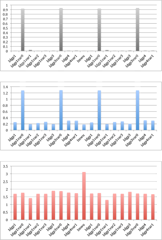
Figure 5: Histogram plots of the statistic $\log(1+\mu)$ whenever $\mu$ is the average of $\Phi$ (top), $\Psi$ (middle), and CPU time (bottom) over all instances, for each relevant combination of solver$+$formulation, with “solver” in MS (left), MWU (middle) and VNS (right).

The statistics for the Mosek solver, limited to instances where $n\leq 200$ because of RAM limitations, are given below.

Formulation	$\Phi$	$\Psi$	CPU
sdprel	0.037	0.516	51
sdprel1	0.123	0.678	45
yajima	0.113	0.717	45

The relevant figure in this table is that the SDP relaxation sdprel has much lower average edge error than the other formulations, lower maximum error, and slightly higher CPU time.

These tests show that, on average, the SDP trace variant, Yajima’s relaxation, and all square root variants are not worth considering. The reason why introducing square roots results in performance losses may be related to the use of the same local subsolver (Ipopt) within all global optimization solver, since it carries out most floating point computations.

A remark about Yajima’s relaxation: although it was introduced specifically for the i DGP, it was originally solved using an ad-hoc interior point method. Even though our results show it underperforms on average with respect to Mosek, this does not negate the (good) results reported in [56].

We call bad the solver$+$formulation combinations we excluded, and good the rest. The good combinations are shown below, marked by a “1” in the corresponding entry.

Formulation			Solver
Description	Notation	Name	MS	MWU	VNS	Mosek
(13)	(13)	Idgp1	1		1
(13) variant (i)	(13).1	Idgp1var1	1		1
(13) variant (ii)	(13).2	Idgp1var2	1		1
(13) variant (iii)	(13).3	Idgp1var3	1		1
(14)	(14)	Idgp3	1		1
(15)	(15)	Idgp4	1		1
(15) variant (i)	(15).1	Idgp4var1	1		1
(19)	(19)	Imwu		1
(17)	(17)	sdprel				1

5.5 Focusing on the hard instances

We also make a qualitative distinction between easy and hard instances. We call an instance easy if at least one third of the good combinations find a solution with $\Phi,\Psi$ approximately zero within 1s of user CPU time, and hard the rest. The classification is reported in the last column of Table 5: hard instances are marked “H”. We marked H^∗ the instances which are “borderline hard”, i.e., there is at least one good combination which finds a solution with $\Phi,\Psi$ approximately zero within 1s of user CPU time.

The computational results below will focus on the hard instances for $\Phi,\Psi$; because of excessive computational requirements, however, we shall relax this constraint for the results on the DEMI measure $\partial$.

5.6 Testing heuristics without averages

When benchmarking heuristic algorithms, such as MS, VNS, or MWU, it is customary to present results based on a number of runs (the higher the better) of the same instance. Because of the complexity of this computational comparison, and the absolute time taken to perform it, it was ungainly for us to multiply this effort by a significant factor (say 10 or 100). Does this mean that our results are unreliable? Though it could be argued that the instance-by-instance results are in fact unreliable, as can be gleaned by the difference in $\partial$ measure for the tiny instance in Sect. 3 and those in Table 10, we think the averages (reported in Tables 7-10) are not. Since we never claim in our computational comparisons that one method is best for a certain instance, but only suggest first and second best over all tested instances, we think our computational benchmark is significant.

5.7 Comparative results on edge errors and CPU

In this section we discuss an overarching comparison yielding an overall “winner”. Our most meaningful measure, if $\Phi$ and $\Psi$ are nonzero, is the DEMI measure $\partial(\cdot,y)$, where $y$ is a given solution of the ^KDMDGP instance being solved. By Sect. 2.3.4, however, we are not able to compute it for every instance, and hence we focus on $\Phi,\Psi$ for our global comparison, and only look at $\delta$ on a subset of instances (Sect. 5.8).

Tables 7-9 report the average edge errors $\Phi$, the maximum edge error $\Psi$, and the CPU time taken by the good combinations when solving hard instances.

Instance	$\mbox{\tt mosek}\atop\mbox{\tt sdprel}$	$\mbox{\tt ms}\atop\mbox{\tt Idgp1}$	$\mbox{\tt ms}\atop\mbox{\tt Idgp1var1}$	$\mbox{\tt ms}\atop\mbox{\tt Idgp1var2}$	$\mbox{\tt ms}\atop\mbox{\tt Idgp1var3}$	$\mbox{\tt ms}\atop\mbox{\tt Idgp3}$	$\mbox{\tt ms}\atop\mbox{\tt Idgp4}$	$\mbox{\tt ms}\atop\mbox{\tt Idgp4var1}$	$\mbox{\tt mwu}\atop\mbox{\tt Imwu}$	$\mbox{\tt vns}\atop\mbox{\tt Idgp1}$	$\mbox{\tt vns}\atop\mbox{\tt Idgp1var1}$	$\mbox{\tt vns}\atop\mbox{\tt Idgp1var2}$	$\mbox{\tt vns}\atop\mbox{\tt Idgp1var3}$	$\mbox{\tt vns}\atop\mbox{\tt Idgp3}$	$\mbox{\tt vns}\atop\mbox{\tt Idgp4}$	$\mbox{\tt vns}\atop\mbox{\tt Idgp4var1}$
100d	NA	0.076	0.208	0.07	0.104	0.124	0.127	0.125	0.0932	0.124	0.222	0.111	0.138	0.124	0.129	0.143
1PPT	NA	0.0925	0.209	0.0969	0.131	0.0742	0.0994	0.107	0.0787	0.0769	0.227	0.07	0.0891	0.0974	0.13	0.164
1guu	NA	0.000348	0.000408	0.000106	0.00242	0.00141	0.0132	0.0188	0.00033	0.00144	0.00129	0.000792	8.33e-05	0.00	0.0134	0.0181
1guu-1	0.297	0.00745	0.012	0.00467	0.00716	0.00	0.0178	0.0102	0.0103	0.00345	0.00682	0.00574	0.0118	0.00319	0.0177	0.0214
1guu-4000	0.285	0.00654	0.0213	0.00401	0.0101	0.00387	0.0201	0.0315	0.0149	0.00704	0.0171	0.0077	0.0216	0.00	0.0158	0.0242
2kxa	NA	0.063	0.432	0.0479	0.045	0.136	0.0711	0.0312	0.01	0.0285	0.34	0.085	0.0676	0.137	0.122	0.0689
C0020pdb	0.02	0.0376	0.148	0.0388	0.0776	0.0464	0.0702	0.062	0.0435	0.0248	0.144	0.0438	0.0452	0.0527	0.079	0.0354
C0030pkl	0.0245	0.0509	0.46	0.042	0.159	0.0374	0.104	0.0802	0.02	0.0456	0.25	0.0329	0.075	0.141	0.0568	0.108
C0080create.1	0.0248	0.00	0.00	0.00	0.00	0.00416	0.00523	0.0049	0.00	0.00	0.121	0.00	0.00	0.034	0.00523	0.00516
C0080create.2	0.0248	0.00	0.0169	0.00	0.00	0.00	0.00523	0.00551	0.00	0.00	0.0306	0.00	0.00387	0.0321	0.00523	0.00486
C0150alter.1	0.0169	0.00	0.00	0.00	0.00	0.00	0.00159	0.00169	0.00	0.00	0.00	0.00	0.00	0.00	0.00159	0.0021
GM1_sugar	0.0187	0.00	0.0525	0.000893	0.015	0.00	0.00504	0.00552	1.92e-06	0.0111	0.0246	0.00	0.00962	0.0279	0.00507	0.00459
cassioli…	NA	0.0345	0.357	0.00	0.0423	0.0485	0.0553	0.0938	0.00685	0.0383	0.191	0.0584	0.0762	0.0797	0.0784	0.0757
helix_amber	NA	0.0451	0.418	0.0516	0.0872	0.0889	0.0523	0.12	0.0453	0.0461	0.324	0.01	0.0574	0.135	0.0848	0.104
lavor30_6-2	0.0643	0.00	0.00	0.00	0.00	0.00	0.0108	0.0157	0.00	0.00	0.00	0.00	0.00	0.00	0.011	0.0134
lavor30_6-3	0.0902	0.00	0.00	0.00	0.00	0.00	0.0101	0.0113	0.00312	0.00	0.00	0.00	0.00	0.00	0.0101	0.00926
lavor30_6-4	0.139	0.00	0.00	0.00	0.00	0.00	0.0103	0.0114	0.00	0.00	0.00	0.00319	0.00	0.00	0.0103	0.013
names	0.0238	0.00658	0.148	0.015	0.0172	0.0566	0.0115	0.00434	0.0142	0.00	0.0877	0.0212	0.0315	0.0688	0.0349	0.00768
pept	0.0419	0.0575	0.104	0.0256	0.0685	0.0339	0.0567	0.0629	0.0755	0.0647	0.114	0.0175	0.0496	0.0517	0.0329	0.01
res_0	NA	0.0318	0.119	0.0248	0.0483	0.0247	0.0727	0.0446	0.0604	0.026	0.163	0.01	0.0552	0.0227	0.0482	0.0478
res_1000	NA	0.02	0.109	0.0373	0.0191	0.0602	0.0811	0.0855	0.0424	0.018	0.191	0.0216	0.0282	0.081	0.0666	0.0526
res_2000	NA	0.0119	0.177	0.0236	0.0397	0.0669	0.0472	0.0524	0.00	0.0496	0.0884	0.0322	0.0215	0.129	0.0688	0.0472
res_2kxa	NA	0.0487	0.14	0.0693	0.051	0.0448	0.0558	0.0792	0.0377	0.0563	0.303	0.0578	0.0963	0.0508	0.02	0.0202
res_3000	NA	0.0347	0.191	0.00338	0.0506	0.0905	0.0539	0.0316	0.00	0.0335	0.0616	0.0256	0.046	0.0471	0.0345	0.0508
res_5000	NA	0.0504	0.158	0.0395	0.0316	0.0231	0.0446	0.0582	0.00	7.91e-05	0.132	0.0355	0.0676	0.121	0.0313	0.0294
tiny	0.0132	0.00	0.00	0.00	0.00	0.00	0.00475	0.0047	0.00	0.00	0.00	0.00	0.00	0.00	0.00475	0.00493
water	NA	0.23	0.492	0.229	0.272	0.336	0.13	0.232	0.227	0.215	0.438	0.212	0.215	0.291	0.163	0.242
Average	0.078	0.033	0.147	0.031	0.047	0.048	0.046	0.052	0.029	0.032	0.129	0.032	0.045	0.064	0.047	0.049

Table 7: $\Phi$ statistics: blue indicates best.

We remark that the MWU algorithm is best with respect to the edge errors $\Phi$ and $\Psi$, and the worst with respect to CPU time. However, since CPU time is of least consequence in protein conformation computations, CPU time information has a much lower priority than solution quality.

Instance	$\mbox{\tt mosek}\atop\mbox{\tt sdprel}$	$\mbox{\tt ms}\atop\mbox{\tt Idgp1}$	$\mbox{\tt ms}\atop\mbox{\tt Idgp1var1}$	$\mbox{\tt ms}\atop\mbox{\tt Idgp1var2}$	$\mbox{\tt ms}\atop\mbox{\tt Idgp1var3}$	$\mbox{\tt ms}\atop\mbox{\tt Idgp3}$	$\mbox{\tt ms}\atop\mbox{\tt Idgp4}$	$\mbox{\tt ms}\atop\mbox{\tt Idgp4var1}$	$\mbox{\tt mwu}\atop\mbox{\tt Imwu}$	$\mbox{\tt vns}\atop\mbox{\tt Idgp1}$	$\mbox{\tt vns}\atop\mbox{\tt Idgp1var1}$	$\mbox{\tt vns}\atop\mbox{\tt Idgp1var2}$	$\mbox{\tt vns}\atop\mbox{\tt Idgp1var3}$	$\mbox{\tt vns}\atop\mbox{\tt Idgp3}$	$\mbox{\tt vns}\atop\mbox{\tt Idgp4}$	$\mbox{\tt vns}\atop\mbox{\tt Idgp4var1}$
100d	NA	3.21	2.09	3.45	3.91	2.47	4.05	3.85	3.05	4.29	2.05	3.9	3.7	2.58	3.62	3.81
1PPT	NA	3.31	2.14	2.87	3.56	2.12	3.53	3.76	2.66	3.28	1.93	4.01	3.0	2.79	3.5	3.71
1guu	NA	0.332	0.0167	0.0667	0.517	0.0603	0.965	1.36	0.143	0.36	0.053	0.345	0.0629	0.00	1.33	1.19
1guu-1	3.2	0.394	0.233	0.45	0.813	0.06	1.23	0.677	0.453	0.38	0.0846	0.44	1.22	0.101	0.948	1.0
1guu-4000	2.97	1.48	0.564	0.912	1.29	0.151	1.49	1.58	0.95	1.27	0.256	1.62	1.75	0.08	1.0	3.03
2kxa	NA	3.62	2.13	3.57	2.7	2.59	3.32	2.38	1.21	3.37	2.01	2.76	3.51	3.04	3.76	3.59
C0020pdb	0.898	1.99	1.86	2.1	2.01	0.89	3.35	2.07	1.45	1.93	1.4	2.48	2.48	0.81	3.22	2.57
C0030pkl	1.27	3.83	2.35	2.75	3.74	1.35	3.59	4.0	1.62	3.51	2.55	3.42	3.72	1.78	3.42	3.58
C0080create.1	0.546	0.00	0.00	0.00	0.00	0.304	0.272	0.254	0.00	0.00	1.71	0.00	0.00	0.953	0.272	0.314
C0080create.2	0.546	0.00	0.406	0.00	0.00	0.00	0.272	0.211	0.00	0.00	0.618	0.00	0.911	1.04	0.272	0.313
C0150alter.1	0.443	0.00	0.00	0.00	0.00	0.00	0.0856	0.176	0.00	0.00	0.00	0.00	0.00	0.00	0.0856	0.142
GM1_sugar	0.474	0.00	0.505	0.32	1.54	0.00	0.31	0.312	0.00117	1.13	0.309	0.00	1.19	0.635	0.55	0.419
cassioli…	NA	3.16	2.59	0.00	3.57	2.64	3.27	3.84	1.67	3.3	2.36	3.39	3.65	1.76	3.54	3.85
helix_amber	NA	3.39	2.69	2.99	3.57	3.65	3.76	3.56	2.77	3.52	2.12	3.39	3.88	2.15	3.84	3.52
lavor30_6-2	0.959	0.00	0.00	0.00	0.00	0.00	0.414	0.418	0.00	0.00	0.00	0.00	0.00	0.00	0.374	0.369
lavor30_6-3	1.42	0.00	0.00	0.00	0.00	0.00	0.4	0.307	0.314	0.00	0.00	0.00	0.00	0.00	0.4	0.332
lavor30_6-4	2.1	0.00	0.00	0.00	0.00	0.00	0.362	0.368	0.00	0.00	0.00	0.314	0.00	0.00	0.362	0.508
names	0.951	0.845	1.86	0.807	1.77	2.26	1.03	0.29	0.928	0.295	1.28	1.7	1.44	1.51	3.09	0.978
pept	1.66	3.43	0.699	1.47	2.59	1.62	2.02	3.02	1.99	2.39	1.96	2.66	3.56	0.887	2.72	0.35
res_0	NA	2.85	1.03	2.89	3.36	0.82	3.02	3.2	2.19	2.47	2.16	2.47	2.1	0.824	3.0	3.11
res_1000	NA	2.49	1.83	2.68	2.59	1.86	2.82	3.21	2.3	2.75	2.04	2.67	2.94	2.3	3.24	2.63
res_2000	NA	1.42	2.26	2.79	2.16	1.2	3.19	2.58	0.00	3.21	1.25	2.07	2.12	2.08	2.62	2.22
res_2kxa	NA	3.29	2.07	3.3	2.81	2.26	2.91	3.17	2.53	3.19	2.42	3.35	3.68	1.65	2.63	2.72
res_3000	NA	2.8	1.35	0.867	3.28	1.78	2.91	3.17	0.00	2.73	1.08	1.87	2.9	1.8	3.09	3.55
res_5000	NA	3.39	2.06	3.66	2.1	1.16	2.8	2.81	0.00	0.11	1.78	2.77	2.55	1.72	2.32	2.68
tiny	0.306	0.00	0.00	0.00	0.00	0.00	0.334	0.318	0.00	0.00	0.00	0.00	0.00	0.00	0.334	0.385
water	NA	4.13	2.66	4.17	4.46	4.9	4.03	3.86	3.77	3.82	2.57	4.3	3.82	4.1	4.23	3.86
Average	1.267	1.828	1.237	1.560	1.939	1.265	2.064	2.028	1.111	1.752	1.259	1.849	2.007	1.281	2.140	2.027

Table 8: $\Psi$ statistics: blue indicates best.

We can therefore make the following claim.

The MWU algorithm is the best solver on average.

Instance	$\mbox{\tt mosek}\atop\mbox{\tt sdprel}$	$\mbox{\tt ms}\atop\mbox{\tt Idgp1}$	$\mbox{\tt ms}\atop\mbox{\tt Idgp1var1}$	$\mbox{\tt ms}\atop\mbox{\tt Idgp1var2}$	$\mbox{\tt ms}\atop\mbox{\tt Idgp1var3}$	$\mbox{\tt ms}\atop\mbox{\tt Idgp3}$	$\mbox{\tt ms}\atop\mbox{\tt Idgp4}$	$\mbox{\tt ms}\atop\mbox{\tt Idgp4var1}$	$\mbox{\tt mwu}\atop\mbox{\tt Imwu}$	$\mbox{\tt vns}\atop\mbox{\tt Idgp1}$	$\mbox{\tt vns}\atop\mbox{\tt Idgp1var1}$	$\mbox{\tt vns}\atop\mbox{\tt Idgp1var2}$	$\mbox{\tt vns}\atop\mbox{\tt Idgp1var3}$	$\mbox{\tt vns}\atop\mbox{\tt Idgp3}$	$\mbox{\tt vns}\atop\mbox{\tt Idgp4}$	$\mbox{\tt vns}\atop\mbox{\tt Idgp4var1}$
100d	NA	612.0	63.30	312.0	375.0	345.0	307.0	319.0	8230.0	316.0	65.2	359.0	290.0	1010.0	441.0	188.0
1PPT	NA	87.1	25.90	52.4	70.8	926.0	55.8	61.0	2292.1	54.9	31.7	62.0	77.6	262.0	98.3	95.7
1guu	NA	21.1	20.1	22.4	20.6	26.6	20.6	20.3	64.3	10.9	20.4	20.9	20.5	6.03	21.5	21.3
1guu-1	1020.0	22.1	20.20	20.7	20.6	21.6	20.7	20.6	70.63	21.1	20.3	22.2	20.5	20.20	20.20	20.20
1guu-4000	816.0	21.1	20.4	22.5	21.9	21.9	22.4	20.6	84.66	21.1	20.4	22.7	21.0	22.9	20.9	20.10
2kxa	NA	26.6	21.90	29.7	31.7	227.0	36.2	32.1	2018.66	101.0	28.6	29.8	30.5	74.3	36.2	50.3
C0020pdb	135.0	22.0	20.2	23.8	20.00	25.3	24.8	22.0	198.66	22.0	21.2	20.8	20.4	20.4	20.8	24.8
C0030pkl	4440.0	60.8	26.1	51.4	47.3	69.8	23.60	54.0	3108.14	51.4	25.0	57.7	85.5	72.8	43.5	27.0
C0080create.1	12.7	4.52	1.22	2.28	2.91	21.4	20.2	20.4	55.31	17.1	2.99	2.81	3.35	21.1	20.2	20.1
C0080create.2	12.7	3.95	20.1	8.1	4.39	3.92	20.5	20.3	51.90	18.3	20.2	2.14	7.24	20.6	20.4	20.1
C0150alter.1	4.32	2.76	1.75	1.28	0.67	1.85	20.2	20.2	17.31	7.72	1.47	0.888	7.66	12.3	7.78	5.57
GM1_sugar	15.6	13.8	20.4	20.7	21.7	9.15	21.3	20.1	53.28	7.83	20.1	20.8	20.0	20.1	20.0	20.4
cassioli…	NA	120.0	33.60	171.0	121.0	572.0	175.0	88.3	7842.0	186.0	34.2	104.0	100.0	67.5	87.5	81.1
helix_amber	NA	210.0	80.30	193.0	147.0	267.0	168.0	112.0	12628.8	222.0	101.0	259.0	209.0	157.0	221.0	91.7
lavor30_6-2	3.04	1.39	1.36	2.12	1.36	1.51	20.0	20.0	7.82	0.444	2.32	0.34	0.427	9.98	4.08	2.52
lavor30_6-3	3.11	2.87	0.8	1.7	0.962	0.68	20.0	20.0	7.18	3.62	1.84	3.14	2.6	11.9	2.61	2.08
lavor30_6-4	3.05	1.34	0.653	1.45	0.31	1.94	20.0	20.0	7.46	1.59	2.67	1.55	6.88	0.332	0.412	0.37
names	44.1	20.4	21.9	21.7	21.4	23.5	21.7	20.5	104.0	22.9	4.59	15.4	22.1	37.4	20.3	20.9
pept	105.0	22.7	21.0	24.9	22.9	22.2	22.7	20.5	171.2	17.40	21.0	23.1	20.2	20.1	20.4	20.3
res_0	NA	20.3	21.6	23.0	22.0	27.1	26.4	20.4	263.51	22.6	21.0	20.7	21.8	24.0	10.10	21.5
res_1000	NA	23.6	23.8	22.6	23.0	21.0	21.1	25.3	342.46	23.3	21.2	22.4	21.5	23.6	21.7	20.60
res_2000	NA	23.0	20.8	26.3	20.6	77.6	21.3	20.7	245.08	22.5	20.5	22.4	20.5	90.8	20.10	21.4
res_2kxa	NA	28.1	20.30	30.5	33.0	43.9	30.2	26.4	1614.6	42.6	24.5	28.5	37.0	31.3	26.7	36.4
res_3000	NA	24.0	20.7	24.0	23.5	28.4	20.6	29.2	270.56	20.7	22.4	22.2	26.5	21.0	20.00	20.00
res_5000	NA	22.0	20.4	22.8	21.0	21.8	21.0	21.0	224.83	24.7	20.6	20.20	22.0	20.4	22.8	21.1
tiny	4.89	2.51	2.11	0.813	4.45	3.19	20.0	20.1	18.16	0.772	3.9	0.686	5.4	0.50	5.51	0.821
water	NA	1530.0	937.0	1800.0	1800.0	1800.0	1800.0	1520.0	38597.0	1800.0	542.00	1800.0	1800.0	1890.0	1600.0	1800.0
Average	472.822	109.261	55.107	108.635	107.409	170.790	111.159	96.852	2910.0	113.351	41.529	109.828	108.154	146.983	105.703	99.050

Table 9: CPU time statistics: blue indicates best.

Given the consequential CPU time difference between MWU and the other solvers, it is worth ranking the solver$+$formulation combinations by $\Phi,\Psi$, and CPU time (see below).

Rank	$\Phi$		$\Psi$		CPU
1	mwu+Imwu	0.029	mwu+Imwu	1.111	vns+Idgp1var1	41.53
2	ms+Idgp1var2	0.031	ms+Idgp1var1	1.237	ms+Idgp1var1	55.11
3	vns+Idgp1	0.032	vns+Idgp1var1	1.259	ms+Idgp4var1	96.85
4	vns+Idgp1var2	0.032	ms+Idgp3	1.265	vns+Idgp4var1	99.05
5	ms+Idgp1	0.033	mosek+sdprel	1.267	vns+Idgp4	105.70
6	vns+Idgp1var3	0.045	vns+Idgp3	1.281	ms+Idgp1var3	107.41
7	ms+Idgp4	0.046	ms+Idgp1var2	1.560	vns+Idgp1var3	108.15
8	ms+Idgp1var3	0.047	vns+Idgp1	1.752	ms+Idgp1var2	108.63
9	vns+Idgp4	0.047	ms+Idgp1	1.828	ms+Idgp1	109.26
10	ms+Idgp3	0.048	vns+Idgp1var2	1.849	vns+Idgp1var2	109.83
11	vns+Idgp4var1	0.049	ms+Idgp1var3	1.939	ms+Idgp4	111.16
12	ms+Idgp4var1	0.052	vns+Idgp1var3	2.007	vns+Idgp1	113.35
13	vns+Idgp3	0.064	vns+Idgp4var1	2.027	vns+Idgp3	146.98
14	mosek+sdprel	0.078	ms+Idgp4var1	2.028	ms+Idgp3	170.79
15	vns+Idgp1var1	0.129	ms+Idgp4	2.064	mosek+sdrel	472.82
16	ms+Idgp1var1	0.147	vns+Idgp4	2.140	mwu+Imwu	27669

This ranking shows that mwu+Imwu has the only consistent ranking in both $\Phi$ and $\Psi$. It also shows that no other solver$+$formulation combination has the same desirable property of approximately equal rank w.r.t. both $\Phi$ and $\Psi$. The issue is not only relative: values of $\Phi$ higher than $0.1$ and of $\Psi$ higher than $1.5$ may well imply that the realization is fundamentally wrong, and the only combinations with $\Phi<0.1$ and $\Psi<1.5$ are ms+Idgp3, vns+Idgp3, mosek+sdprel. However, the statistics for the latter were computed on a subset of instances (all those with $n\leq 200$) due to the high RAM requirements of Mosek when applied to large instances (see Sect. 5.4). Based on these observations, we claim that:

the formulation Idgp3 in Eq. (14), when used with MS or VNS, is second best.

We observe that the usual trade-off between quality and efficiency is also at play: solving Eq. (14) takes longest over all formulations solved by both MS and VNS.

5.8 Results on DEMI

Table 10 reports the results on the DEMI measure. Note that the instances in the test set are not the same as for the tests on $\Phi,\Psi$, and CPU (Tables 7-9). As mentioned in Sect. 2.3.4, it is not always possible to determine a cTOP order automatically (or disprove that one exists) in acceptable amounts of CPU time, which is a requirement for computing the DEMI measure. Table 10 includes all instances for which this task could be carried out within 150s of CPU time.

Although it is clear that the SDP relaxation Eq. (17) scores the best performance in terms of the DEMI measure, we mentioned above that the Mosek solver is unable to scale up to desired sizes. We must therefore resort to the second best, which happens to be the MWU algorithm, consistently with Sect. 5.7. We also observe that VNS attains lower average DEMI measure values more often than MS.

We recall that the DEMI measure values for tiny differ from those given in Sect. 3 for the reasons given in Sect. 5.6.

6 Conclusion

Our main aim is to find the best general-purpose continuous search methods for solving i DGP instances. To answer this question, we need: (i) a set of benchmarking measures; (ii) a set of i DGP formulations; (iii) a set of methods; (iv) extensive computational results. Since a preliminary study [33] showed that two standard metaheuristics and the existing benchmark measures were insufficient, we decided to introduce a new measure and a new method.

Accordingly, this paper presents several notions: (a) a coordinate root mean square deviation modulo partial reflections (called DEMI measure), for benchmarking the performance of i DGP algorithms on protein isomers; (b) a zoo of mathematical programming formulations for the i DGP; (c) a new method for solving the i DGP, based on the well-known Multiplicative Weights Update (MWU) algorithm; (d) a complex computational benchmark for the best formulation-based methods on the hardest instances.

Our study shows that, on average:

• the new MWU-based heuristic yields i DGP solutions of highest quality with respect to existing measures;

• the Square Factoring formulation in Eq. (14) is second best;

• as concerns the new DEMI measure, the SDP relaxation in Eq. (17) is best, but only on a limited set of instances, whereas the MWU-based heuristic is second best.

Future research directions for the topics presented in this paper include: (i) the algorithmic exploitation of the DEMI measure for more effective pruning within the Branch-and-Prune algorithm; (ii) the insertion of a limited diving device within the Branch-and-Prune: instead of branching in order to find possible positions of the next atom in the order, it would be desirable to realize a considerable number of successive atoms by means of one of the continuous methods presented in this paper.

Instance	$\mbox{\tt mosek}\atop\mbox{\tt sdprel}$	$\mbox{\tt ms}\atop\mbox{\tt Idgp1}$	$\mbox{\tt ms}\atop\mbox{\tt Idgp1var1}$	$\mbox{\tt ms}\atop\mbox{\tt Idgp1var2}$	$\mbox{\tt ms}\atop\mbox{\tt Idgp1var3}$	$\mbox{\tt ms}\atop\mbox{\tt Idgp3}$	$\mbox{\tt ms}\atop\mbox{\tt Idgp4}$	$\mbox{\tt ms}\atop\mbox{\tt Idgp4var1}$	$\mbox{\tt mwu}\atop\mbox{\tt Imwu}$	$\mbox{\tt vns}\atop\mbox{\tt Idgp1}$	$\mbox{\tt vns}\atop\mbox{\tt Idgp1var1}$	$\mbox{\tt vns}\atop\mbox{\tt Idgp1var2}$	$\mbox{\tt vns}\atop\mbox{\tt Idgp1var3}$	$\mbox{\tt vns}\atop\mbox{\tt Idgp3}$	$\mbox{\tt vns}\atop\mbox{\tt Idgp4}$	$\mbox{\tt vns}\atop\mbox{\tt Idgp4var1}$
1guu-1	132.083	116.038	163.411	145.938	158.154	256.755	127.979	196.529	132.709	121.270	112.595	248.200	242.633	313.398	182.382	98.386
1guu	228.757	202.573	210.966	181.700	138.726	209.438	184.057	161.057	153.964	135.907	218.604	172.713	126.893	215.186	201.001	242.788
2erl-frag-bp1	4.203	0.205	26.066	26.118	26.119	26.119	2.841	2.302	0.208	26.119	0.210	0.221	10.312	16.053	2.841	3.403
2kxa	7.954	104.331	109.387	59.612	107.329	74.355	138.700	64.190	15.169	51.538	98.227	152.011	104.147	82.440	101.206	106.075
C0150alter.1	2.105	0.511	0.403	3.412	0.610	0.522	3.028	2.158	0.564	2.598	0.246	5.464	0.240	0.250	3.028	2.910
C0700.odd.G	5.690	38.839	15.052	27.131	15.474	15.159	9.485	7.726	35.427	23.890	0.848	7.142	15.183	2.549	9.485	4.876
C0700.odd.H	5.690	0.520	7.389	7.809	7.391	15.156	9.485	29.485	9.005	27.733	0.422	25.227	0.462	17.623	9.485	10.781
C0700odd.C	5.566	38.284	26.107	49.372	26.033	2.191	20.498	28.260	18.467	25.222	19.999	58.306	24.686	24.708	20.498	27.363
C0700odd.D	5.566	1.795	24.602	40.674	20.131	21.033	30.645	33.841	26.072	21.885	19.998	36.257	19.982	1.799	30.645	26.527
C0700odd.E	5.566	40.742	3.314	57.546	19.257	26.192	30.645	31.231	21.049	19.770	4.451	23.424	24.777	24.647	20.498	13.691
lavor11_7-1	5.970	4.326	0.067	6.800	3.813	0.057	3.232	1.886	4.274	2.203	0.047	4.267	0.109	0.056	3.232	2.752
lavor11_7-2	6.509	0.066	0.076	0.649	1.154	0.079	2.924	2.901	7.366	0.084	0.080	0.485	0.348	0.075	2.924	1.048
lavor11_7-b	5.970	4.274	5.905	3.730	4.273	0.058	3.232	3.237	4.277	0.379	0.681	1.487	0.603	0.096	3.232	2.874
lavor11_7	5.970	0.194	0.072	0.064	0.215	2.130	3.232	3.538	6.555	0.076	0.053	4.028	0.064	0.056	3.232	3.653
lavor11	5.103	0.135	0.128	7.131	4.966	0.942	2.960	7.190	6.642	0.077	6.634	5.603	6.638	0.136	2.960	5.932
lavor30_6-1	32.441	32.157	13.647	30.050	13.649	14.926	21.203	24.563	26.190	14.949	2.286	35.156	16.135	15.448	21.203	22.334
lavor30_6-2	28.787	8.366	10.833	1.565	0.253	11.120	25.772	24.558	29.555	28.764	10.835	0.241	17.135	0.243	12.306	8.709
lavor30_6-3	37.932	42.267	16.883	34.249	30.305	34.248	41.663	7.342	55.839	41.242	16.878	38.034	2.153	16.082	41.663	34.898
lavor30_6-4	16.717	5.142	18.835	12.490	4.558	7.403	5.436	4.149	18.840	1.045	15.509	16.838	15.494	10.353	5.436	19.329
lavor30_6-5	22.715	31.712	15.159	25.267	1.847	26.029	26.834	26.800	44.336	23.498	1.838	15.800	13.133	16.565	26.834	28.453
lavor30_6-7	32.540	41.196	2.035	41.597	2.443	32.357	29.950	17.784	52.537	42.098	40.102	41.153	2.035	20.193	29.950	43.134
lavor30_6-8	10.389	44.385	2.041	42.796	44.901	12.187	45.894	48.735	44.294	44.276	2.136	24.175	2.086	29.897	45.894	46.677
mdgp4-heuristic	0.460	0.894	0.190	0.120	0.557	0.116	0.460	0.460	0.445	0.338	0.345	0.037	0.655	0.119	0.460	0.460
mdgp4-optimal	1.423	0.054	0.066	0.037	0.038	0.026	0.660	0.660	0.707	0.463	0.224	0.033	0.033	0.025	0.660	0.660
res_0	7.933	206.560	149.633	120.930	157.351	46.055	101.755	92.769	75.056	136.851	137.643	149.057	131.249	196.041	79.722	136.753
res_1000	8.151	24.677	82.179	99.962	170.710	122.709	114.645	142.391	99.926	46.920	119.482	85.413	38.340	77.778	121.924	60.485
res_2000	13.866	202.930	125.860	130.671	176.975	97.516	139.965	111.010	0.732	41.158	115.147	95.563	175.189	86.838	134.238	118.871
res_2kxa	11.008	106.131	72.845	94.618	82.791	145.808	83.657	90.800	149.216	110.327	90.640	64.137	118.709	104.359	38.168	35.297
res_3000	9.294	144.285	106.614	48.903	93.328	82.502	80.058	38.559	9.557	117.402	44.590	134.721	70.533	121.108	36.592	165.878
res_5000	7.633	101.283	122.206	105.803	51.874	100.349	99.724	102.613	6.202	44.859	125.495	99.729	61.313	103.984	44.655	82.487
small02	5.566	31.324	14.138	23.329	23.036	25.506	20.498	28.181	2.307	57.688	24.687	62.995	24.689	23.558	30.645	17.314
tiny	2.397	17.715	5.758	18.174	2.189	18.246	2.651	3.720	21.402	4.406	8.322	11.334	7.218	1.864	2.651	7.964
Averages	681.954	1593.911	1351.867	1448.247	1390.450	1427.289	1413.768	1340.625	1078.889	1215.035	1239.254	1619.251	1273.176	1523.527	1269.650	1382.762

Table 10: DEMI measure statistics: blue indicates best. Although the best on average is Mosek on sdprel, this combination was unable to scale up to desired sizes. We therefore also emphasized the second best: MWU on Imwu.

References

- [1] A. Alfakih, A. Khandani, and H. Wolkowicz. Solving Euclidean distance matrix completion problems via semidefinite programming. Computational Optimization and Applications, 12:13–30, 1999.
- [2] H. Alt, K. Mehlhorn, H. Wagener, and E. Welzl. Congruence, similarity and symmetries of geometric objects. Discrete Computational Geometry, 3:237–256, 1988.
- [3] S. Arora, E. Hazan, and S. Kale. Fast algorithms for approximate semidefinite programming using the multiplicative weights update method. In Foundations of Computer Science, volume 46 of FOCS, pages 339–348. IEEE, 2005.
- [4] S. Arora, E. Hazan, and S. Kale. The multiplicative weights update method: a meta-algorithm and applications. Theory of Computing, 8:121–164, 2012.
- [5] M. Atkinson. An optimal algorithm for geometrical congruence. Journal of Algorithms, 8:159–172, 1987.
- [6] A. Bahr, J. Leonard, and M. Fallon. Cooperative localization for autonomous underwater vehicles. International Journal of Robotics Research, 28(6):714–728, 2009.
- [7] S. Basu, R. Pollack, and M.-F. Roy. Algorithms in real algebraic geometry. Springer, New York, 2006.
- [8] N. Beeker, S. Gaubert, C. Glusa, and L. Liberti. Is the distance geometry problem in NP? In Mucherino et al. [49].
- [9] P. Belotti, J. Lee, L. Liberti, F. Margot, and A. Wächter. Branching and bounds tightening techniques for non-convex MINLP. Optimization Methods and Software, 24(4):597–634, 2009.
- [10] R. Benedetti and J.-J. Risler. Real algebraic and semi-algebraic sets. Hermann, Paris, 1990.
- [11] H. Berman, J. Westbrook, Z. Feng, G. Gilliland, T. Bhat, H. Weissig, I.N. Shindyalov, and P. Bourne. The protein data bank. Nucleic Acid Research, 28:235–242, 2000.
- [12] P. Biswas. Semidefinite programming approaches to distance geometry problems. PhD thesis, Stanford University, 2007.
- [13] P. Biswas, T. Lian, T. Wang, and Y. Ye. Semidefinite programming based algorithms for sensor network localization. ACM Transactions in Sensor Networks, 2:188–220, 2006.
- [14] P. Biswas, T.-C. Liang, K.-C. Toh, T.-C. Wang, and Y. Ye. Semidefinite programming approaches for sensor network localization with noisy distance measurements. IEEE Transactions on Automation Science and Engineering, 3:360–371, 2006.
- [15] E. Candès, T. Strohmer, and V. Voroninski. PhaseLift: Exact and stable signal recovery from magniture measurements via convex programming. Communications on Pure and Applied Mathematics, 66(8):1241–1274, 2012.
- [16] A. Cassioli, B. Bordeaux, G. Bouvier, A. Mucherino, R. Alves, L. Liberti, M. Nilges, C. Lavor, and T. Malliavin. An algorithm to enumerate all possible protein conformations verifying a set of distance constraints. BMC Bioinformatics, page 16:23, 2015.
- [17] A. Cassioli, O. Günlük, C. Lavor, and L. Liberti. Discretization vertex orders for distance geometry. Discrete Applied Mathematics, 197:27–41, 2015.
- [18] COIN-OR. Introduction to IPOPT: A tutorial for downloading, installing, and using IPOPT, 2006.
- [19] E. Coutsias, C. Seok, and K. Dill. Using quaternions to calculate rmsd. Journal of Computational Chemistry, 25(15):1849–1857, 2004.
- [20] C. D’Ambrosio, Vu Khac Ky, C. Lavor, L. Liberti, and N. Maculan. Computational experience on distance geometry problems 2.0. In L. Casado, I. Garcia, and E. Hendrix, editors, Mathematical and applied Global Optimization, volume XII of Global Optimization Workshop, pages 97–100, Malaga, 2014. University of Malaga.
- [21] Y. Ding, N. Krislock, J. Qian, and H. Wolkowicz. Sensor network localization, Euclidean distance matrix completions, and graph realization. Optimization and Engineering, 11:45–66, 2010.
- [22] H. Du, N. Alechina, K. Stock, and M. Jackson. The logic of NEAR and FAR. In T. Tenbrink et al., editor, COSIT, volume 8116 of LNCS, pages 475–494, Switzerland, 2013. Springer.
- [23] R. Fourer and D. Gay. The AMPL Book. Duxbury Press, Pacific Grove, 2002.
- [24] C. Goodall. Procrustes methods in the statistical analysis of shape. Journal of the Royal Statistical Society B, 53(2):285–339, 1991.
- [25] L. Henneberg. Die Graphische Statik der starren Systeme. Teubner, Leipzig, 1911.
- [26] C. Lavor. On generating instances for the molecular distance geometry problem. In L. Liberti and N. Maculan, editors, Global Optimization: from Theory to Implementation, pages 405–414. Springer, Berlin, 2006.
- [27] C. Lavor, R. Alves, W. Figuereido, A. Petraglia, and N. Maculan. Clifford algebra and the discretizable molecular distance geometry problem. Advances in Applied Clifford Algebras, 25:925–942, 2015.
- [28] C. Lavor, J. Lee, A. Lee-St. John, L. Liberti, A. Mucherino, and M. Sviridenko. Discretization orders for distance geometry problems. Optimization Letters, 6:783–796, 2012.
- [29] C. Lavor, L. Liberti, N. Maculan, and A. Mucherino. The discretizable molecular distance geometry problem. Computational Optimization and Applications, 52:115–146, 2012.
- [30] C. Lavor, L. Liberti, and A. Mucherino. The interval Branch-and-Prune algorithm for the discretizable molecular distance geometry problem with inexact distances. Journal of Global Optimization, 56:855–871, 2013.
- [31] L. Liberti. Reformulations in mathematical programming: Definitions and systematics. RAIRO-RO, 43(1):55–86, 2009.
- [32] L. Liberti and M. Dražic. Variable neighbourhood search for the global optimization of constrained NLPs. In Proceedings of GO Workshop, Almeria, Spain, 2005.
- [33] L. Liberti and C. Lavor. Solving large-scale distance geometry problems exactly versus approximately. In Optimization Society, Proceedings of the Annual Conference, Houston, 2014. INFORMS.
- [34] L. Liberti, C. Lavor, J. Alencar, and G. Abud. Counting the number of solutions of kDMDGP instances. In F. Nielsen and F. Barbaresco, editors, Geometric Science of Information, volume 8085 of LNCS, pages 224–230, New York, 2013. Springer.
- [35] L. Liberti, C. Lavor, and N. Maculan. A branch-and-prune algorithm for the molecular distance geometry problem. International Transactions in Operational Research, 15:1–17, 2008.
- [36] L. Liberti, C. Lavor, N. Maculan, and A. Mucherino. Euclidean distance geometry and applications. SIAM Review, 56(1):3–69, 2014.
- [37] L. Liberti, C. Lavor, and A. Mucherino. The discretizable molecular distance geometry problem seems easier on proteins. In Mucherino et al. [49].
- [38] L. Liberti, C. Lavor, A. Mucherino, and N. Maculan. Molecular distance geometry methods: from continuous to discrete. International Transactions in Operational Research, 18:33–51, 2010.
- [39] L. Liberti, B. Masson, C. Lavor, J. Lee, and A. Mucherino. On the number of realizations of certain Henneberg graphs arising in protein conformation. Discrete Applied Mathematics, 165:213–232, 2014.
- [40] L. Liberti and L. Mencarelli. A multiplicative weights update algorithm for MINLP, 2014. Working paper.
- [41] L. Liberti, N. Mladenović, and G. Nannicini. A recipe for finding good solutions to MINLPs. Mathematical Programming Computation, 3:349–390, 2011.
- [42] J. Löfberg. YALMIP: A toolbox for modeling and optimization in MATLAB. In Proceedings of the International Symposium of Computer-Aided Control Systems Design, volume 1 of CACSD, Taipei, 2004. IEEE.
- [43] V. Maiorov and G. Crippen. Significance of root-mean-square deviation in comparing three-dimensional structures of globular proteins. Journal of Molecular Biology, 235:625–634, 1994.
- [44] T. Malliavin, A. Mucherino, and M. Nilges. Distance geometry in structural biology. In Mucherino et al. [49].
- [45] The MathWorks, Inc., Natick, MA. MATLAB R2014a, 2014.
- [46] J. Milnor. Topology from the differentiable viewpoint. University Press of Virginia, Charlottesville, 1969.
- [47] J. Moré and Z. Wu. Distance geometry optimization for protein structures. Journal of Global Optimization, 15:219–234, 1999.
-
[48]
Mosek ApS.
The mosek manual, Version 7 (Revision 114), 2014.
(www.mosek.com). - [49] A. Mucherino, C. Lavor, L. Liberti, and N. Maculan, editors. Distance Geometry: Theory, Methods, and Applications. Springer, New York, 2013.
- [50] S. Plotkin, D. Shmoys, and É. Tardos. Fast approximation algorithm for fractional packing and covering problems. Mathematics of Operations Research, 20:257–301, 1995.
- [51] J. Saxe. Embeddability of weighted graphs in -space is strongly NP-hard. Proceedings of 17th Allerton Conference in Communications, Control and Computing, pages 480–489, 1979.
- [52] A. Singer. Angular synchronization by eigenvectors and semidefinite programming. Applied and Computational Harmonic Analysis, 30:20–36, 2011.
- [53] T.-S. Tay and W. Whiteley. Generating isostatic frameworks. Structural Topology, 11:21–69, 1985.
- [54] A. Wächter and L. Biegler. On the implementation of an interior-point filter line-search algorithm for large-scale nonlinear programming. Mathematical Programming, 106(1):25–57, 2006.
- [55] Wikipedia. Variance, Sum of correlated variables, 2016. [Online; accessed 160622].
- [56] Y. Yajima. Positive semidefinite relaxations for distance geometry problems. Japan Journal of Industrial and Applied Mathematics, 19:87–112, 2002.