Microcalorimeter pulse analysis by means of principle component decomposition

Abstract

The X-ray integral field unit for the Athena mission consists of a microcalorimeter transition edge sensor pixel array. Incoming photons generate pulses which are analyzed in terms of energy, in order to assemble the X-ray spectrum. Usually this is done by means of optimal filtering in either time or frequency domain.

In this paper we investigate an alternative method by means of principle component analysis. This method attempts to find the main components of an orthogonal set of functions to describe the data.

We show, based on simulations, what the influence of various instrumental effects is on this type of analysis. We compare analyses both in time and frequency domain. Finally we apply these analyses on real data, obtained via frequency domain multiplexing readout.

1 INTRODUCTION

The proposed X-ray integral field unit (X-IFU)[1] for the Athena[2] mission uses a microcalorimeter array as a 2-dimensional detection device, capable of retrieving high resolution spectra for each imaging element. Each pixel contains a transition edge sensor (TES) which records the energy pulses of incoming X-ray photons. The XIFU detector will have of order 4000 pixels in the array. At SRON we develop a TES-pixel readout scheme by means of frequency domain multiplexing [3].

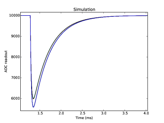
Figure 1: Shape of ideal model pulses, without any systematic instrumental effects, but with some independent noise added. The energy of the pulses is drawn from the expected Mn-K_α distribution

The recorded pulses will have to be analyzed in terms of incoming photon energy. Usually this is done by means of optimal filtering[4], fitting a pulse shape in the time, or frequency domain using appropriate weights based on the noise spectrum. In this paper we use an alternate way of processing by means of principle component analysis (PCA). PCA attempts to find the main components in an orthogonal set of shapes (eigenvectors) which describe the measured pulses. The main eigenvalues, or projections of the pulse onto the main eigenvectors, will have a relation with the incoming photon energy. Ideally only one main component should represent energy and the other components should represent other effects present in the data, but in practice several parameters are mixed in the different components. Projecting a data vector onto an eigenvector (the in-product) can also be seen as multiplying the data vector with a weights vector. As such the PCA method can be seen as a modification of the optimal filtering method, in the sense that PCA derives a best set of weights instead of taking them directly from noise spectrum, for a (set of) component(s) which measure the energy.

Previously Busch et al.[5] have reported on the application of this method to real microcalorimeter data pulses of photons, in time domain DC readout mode. They found this method to be quite promising to obtain the best energy resolution.

Here we report on the application of this method to simulated data, in order to investigate the relation of different effects present in the data on the components found by PCA. In addition we apply PCA to microcalorimeter data obtained at SRON from a multi-pixel array by means of frequency domain multiplexing (FDM). We compare analyses both in time and frequency domain. We aim to minimize the number of relevant components, ideally to obtain the smallest set of components which relate to the energy of the photons, in other words, to maximize the isolation of a component representing the energy.

2 DATA SIMULATION

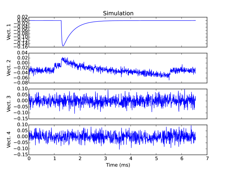
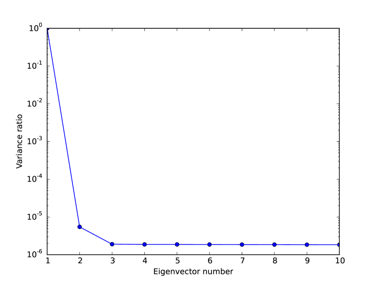
Figure 2: PCA components of ideal pulses. Only the first component, which resembles the pulse shape, and which corresponds to energy is relevant.

Figure 3: Variance ratio of the ideal pulse components, which corresponds to the relative importance. Only the first component matters.

For the simulations, energies are drawn at random from a distribution function for the Mn-K_α X-ray line as published by Holzer[6]. Pulses are generated using exponential rise and fall times representing the SRON detectors and are scaled according to energy. This signal represents the ideal case. On top of this, instrumental effects are added:

• The baseline level is modified using a drifting linear slope and offset

• A drifting gain factor which changes the pulse level plus a partial offset

• A changing pulse start time, correlated with the energy, to mimic the constant trigger threshold with respect to the changing amplitude of the pulse

• A non-linear, saturation relation between input and ’recorded’ signal

• Added noise to the signal

These modifications can be given any magnitude to study the effect of these disturbances on the components found by the PCA. The results of the PCA are analyzed in terms of the fitted instrumental resolution (convolution width) on top of the Holzer[6] natural line width. The fitting method uses the C-stat[7, 8] statistics to cope with the limited number of counts in each spectral bin.

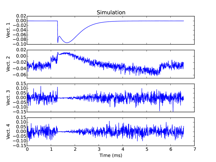
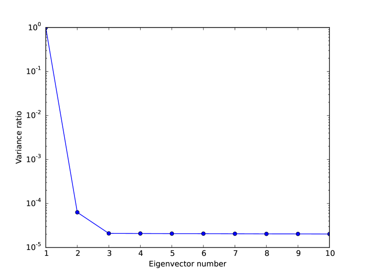
Figure 4: PCA components of saturated pulses.

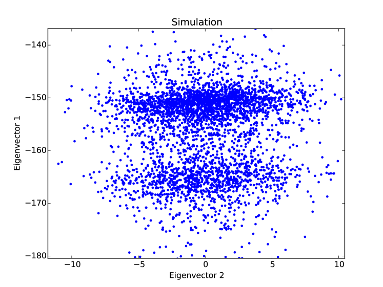
Figure 5: Variance ratio of the saturated pulse components

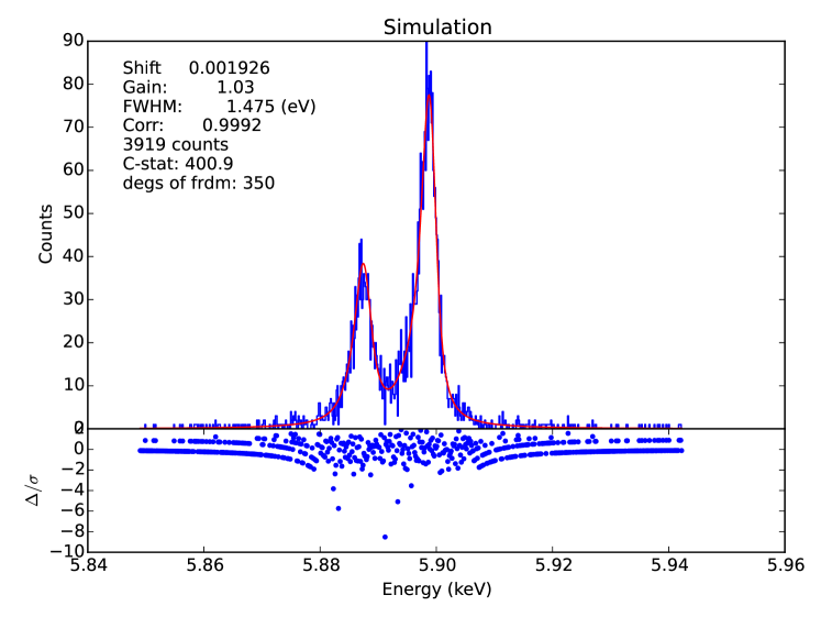
Figure 6: Correlation between the first two PCA components.

Figure 7: Fit of the instrumental resolution on the Mn-K_α line.

Figure 1 shows the ideal modelled pulse shape. PCA analysis (fig 3) shows that only one component is relevant (fig 3). This first component appears like a copy of the basic pulse shape. There appears to be some structure in the second component, but its relevance is only $5\times 10^{-6}$ with respect to the first component. In addition, this relevance can be lowered to any arbitrary low number by decreasing the noise level. This is to be expected, since the only parameters which discriminates the pulses is the energy, and no further instrumental effects are present. The fitted instrumental resolution on the Mn-K_α lines is consistent with no instrumental broadening effect (0.0 eV).

When saturating effects (fig 7) in the signal are introduced, things start to look different. Relevance of the second component now rises to $6\times 10^{-5}$ (fig. 7). The shape of the first component also changes, and there is a slight correlation between first and second components (fig. 7). Instrumental resolution is now fitted at 1.5 eV.

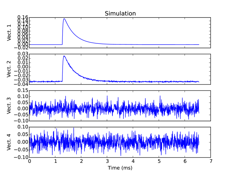
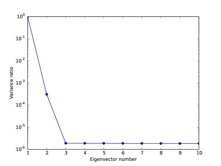
Figure 8: PCA components of pulses subject to gain drifts.

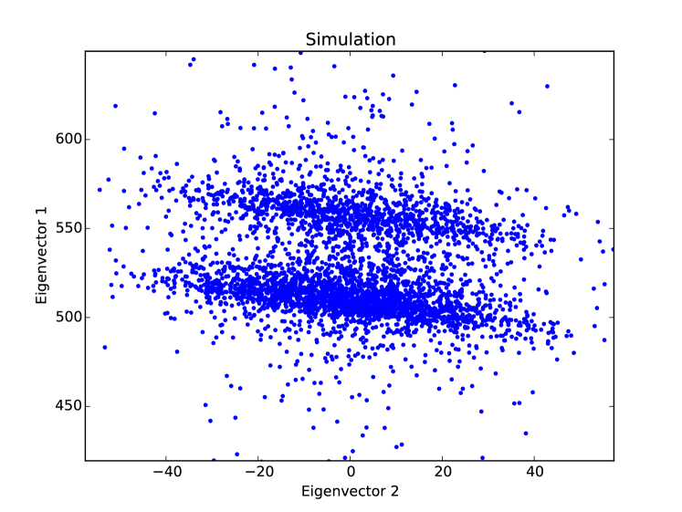
Figure 9: Variance ratio of the gain drift pulses

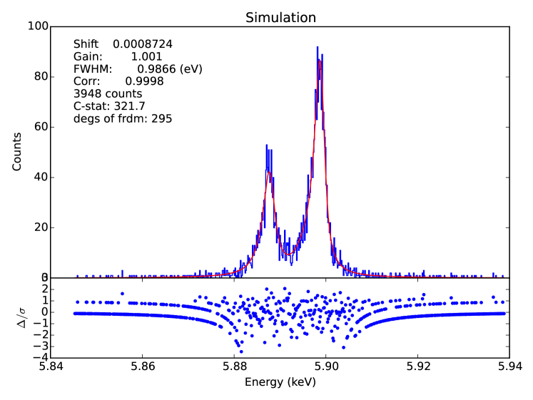
Figure 10: Correlation between the first two PCA components.

Figure 11: Fit of the instrumental resolution on the Mn-K_α line.

Gain drifts show their effects in figures 11 to 11. The second component also matters here at a level of $3\times 10^{-4}$, but the PCA is quite able to cope with this effect. Final instrumental resolution is fitted at about 1 eV.

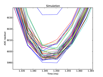
Figure 12: Differences between identical pulses, as shown on the top of the pulse, due to the unequal moments of sampling the pulses.

Final effect is a drift of the pulse with respect to the sampling times. When the pulse is not highly over sampled, the actual pulse shape seems to differ (see figure12). This does not mean that the pulse is under sampled, since proper interpolation can restore the correct pulse form at any position. However this requires significant additional computing resources. With this effect the direct PCA in time domain breaks down. Figures 16 to 16 show the effects for very limited drifts. More than two components now become relevant. There is also clear correlation between the first and second components and this correlation is not linear (fig. 16). Instrumental resolution suffers (2.8 eV, fig. 16).

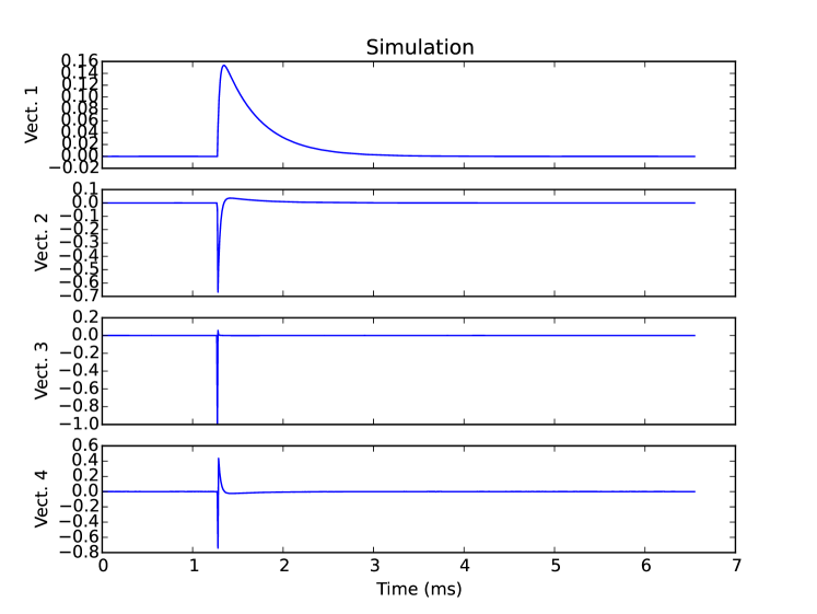
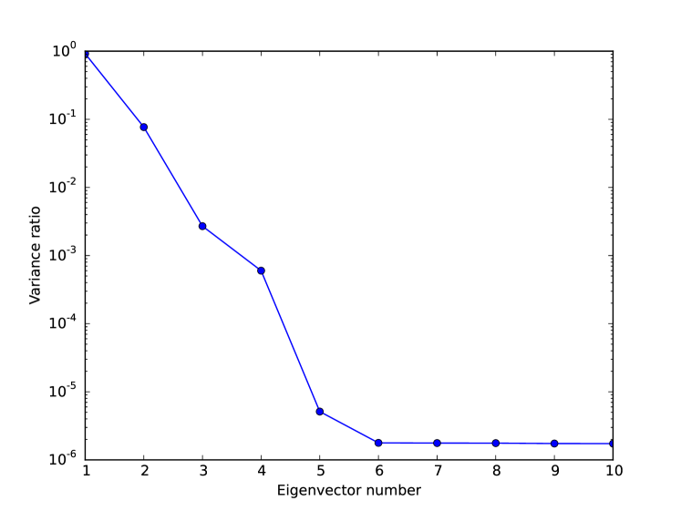
Figure 13: PCA components of pulses subject to sampling jitter.

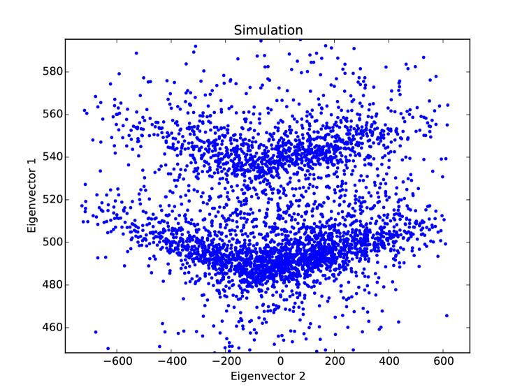
Figure 14: Variance ratio of the sampling jitter pulses

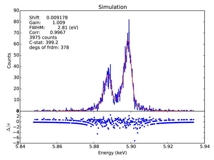
Figure 15: Correlation between the first two PCA components.

Figure 16: Fit of the instrumental resolution on the Mn-K_α line.

3 FREQUENCY DOMAIN ANALYSIS

Apart from analysis in the time domain, PCA can also be done in the frequency domain. Using the power spectrum of the pulse instead of the pulse itself, has the advantage that the phase of the pulse becomes irrelevant. This is confirmed in the simulation analysis. Using the same simulation parameters as before, in the case of saturation and gain drifts the PCA analyses in the frequency domain do not make much difference. Although in the relative importance of the various components only the first component plays a role and other components are all at the same low level (around or below $1\times 10^{-5}$, see figures 18 and 18) the final instrumental resolutions obtained are similar to the time domain case above.

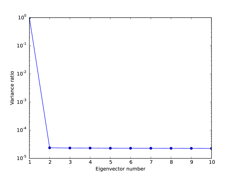
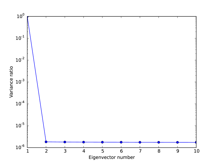
Figure 17: Relative importance of components for the saturated pulses, analyzed in the frequency domain. Compare figure 7 for the time domain. The second component is now significantly lower and at the same level as the higher components.

Figure 18: Relative importance of components for the gain drifted pulses, analyzed in the frequency domain. Compare figure 11 for the time domain. The second component is now significantly lower and at the same level as the higher components.

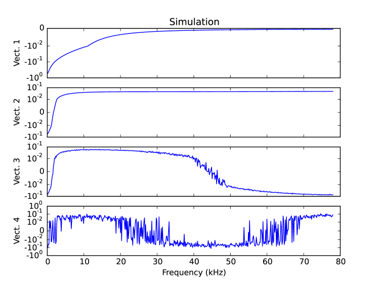
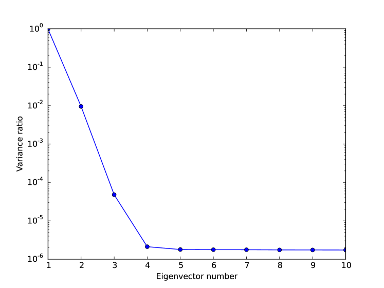
Figure 19: PCA components of pulses subject to sampling jitter, analyzed in frequency domain.

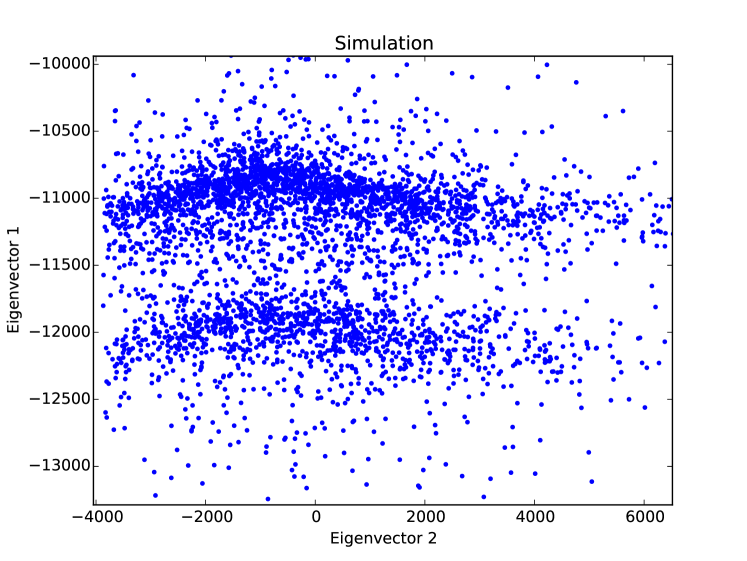
Figure 20: Variance ratio of the sampling jitter pulses in frequency domain.

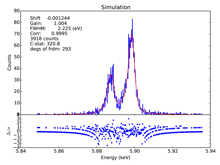
Figure 21: Correlation between the first two PCA frequency domain components.

Figure 22: Fit of the instrumental resolution on the Mn-K_α line.

The major difference is in the pulses with the sample drifts (figures 22 to 22). Since the drifts only affect the position, or phase of the pulse, in frequency domain the effect of this drift is suppressed. The higher components are at least a factor of 10 lower then for the time domain (fig 22). Some correlation between the first components still exists (fig. 22), but the final instrumental resolution obtained is significantly better (2.2 eV, see fig. 22).

4 APPLICATION TO REAL DATA

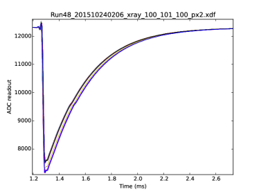
Figure 23: Sample of real pulses from a pixel array read out by means of frequency domain multiplexing. The onset of the pulse is disturbed by a high frequency oscillation.

A set of data was obtained from one pixel within a pixel array, on which multiple pixels were read out by means of frequency domain multiplexing. The readout circuit was not ideal, in the sense that the onset of the pulse was disturbed by a high frequency oscillation (see figure 23). This cause of this is still under investigation. The noise NEP of the signal was around 2.3 eV.

PCA analysis was done both in time domain and frequency domain. Figures 27 to 27 show the time domain results while figures 31 to 31 show the frequency domain results. Here, the time domain analysis completely breaks down, while the frequency domain analysis yields acceptable results. It appears the frequency domain PCA yields about (within the uncertainty of around 0.1 eV) the same final instrumental resolution as the standard optimal filtering in the frequency domain. Depending on sampling frequency, analysis in the frequency domain does have clear advantages.

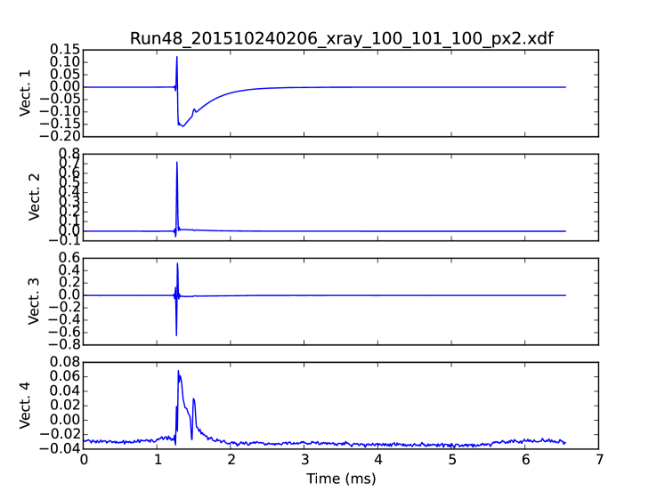
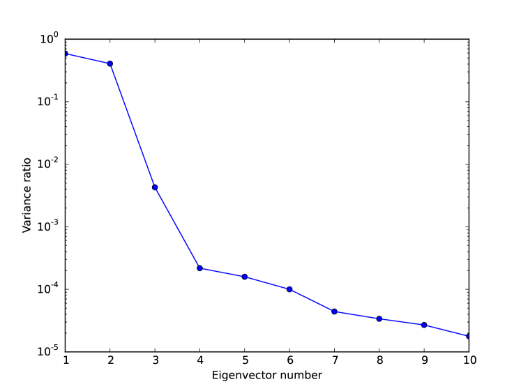
Figure 24: PCA components of real data pulses in time domain.

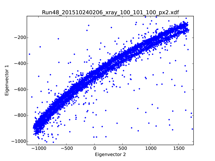
Figure 25: Variance ratio of the real data pulse components

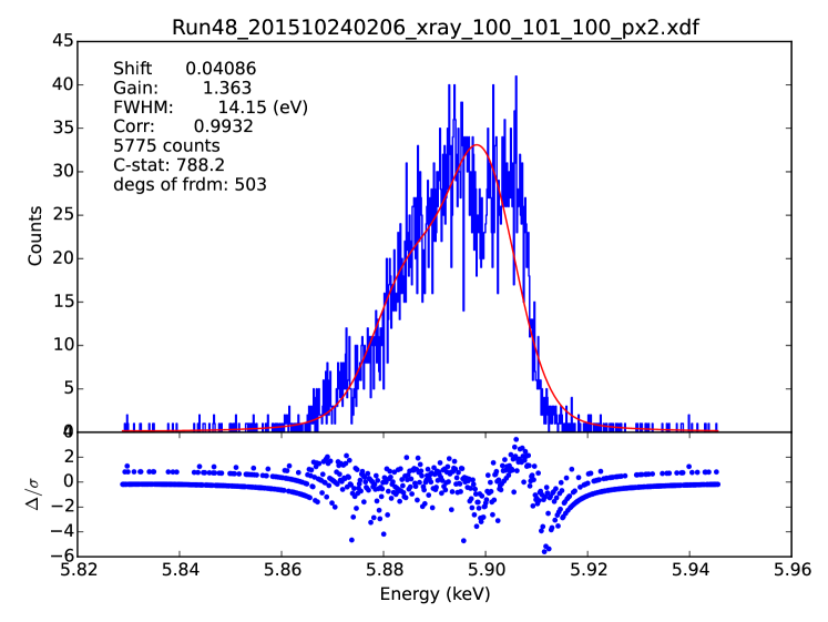
Figure 26: Correlation between the first two PCA components.

Figure 27: Fit of the instrumental resolution on the Mn-K_α line, on the time domain PCA analysis. Clearly this time domain analysis shows bad instrumental resolution.

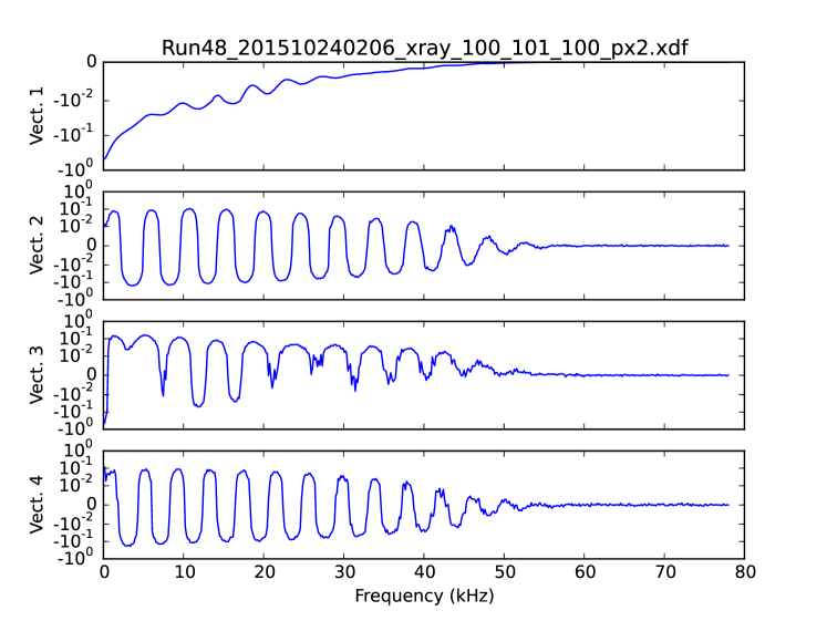
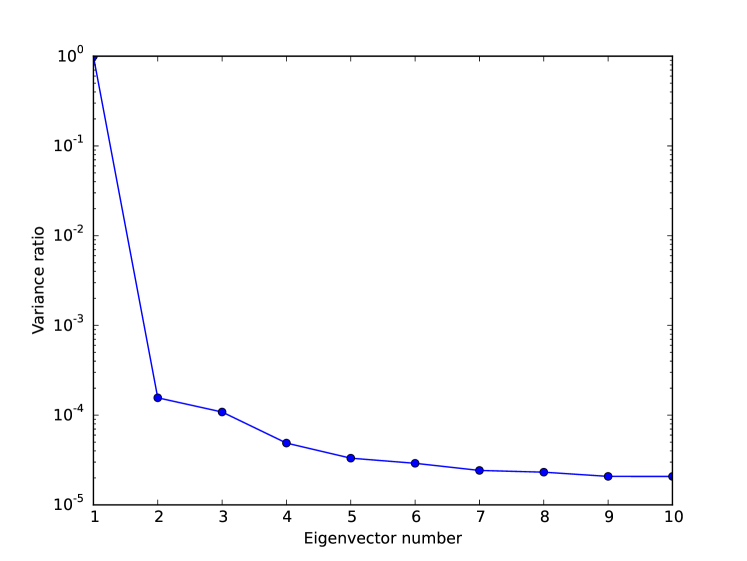
Figure 28: PCA components of real data pulses in frequency domain.

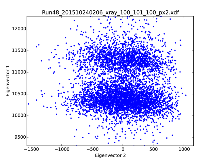
Figure 29: Variance ratio of the real data pulses in frequency domain

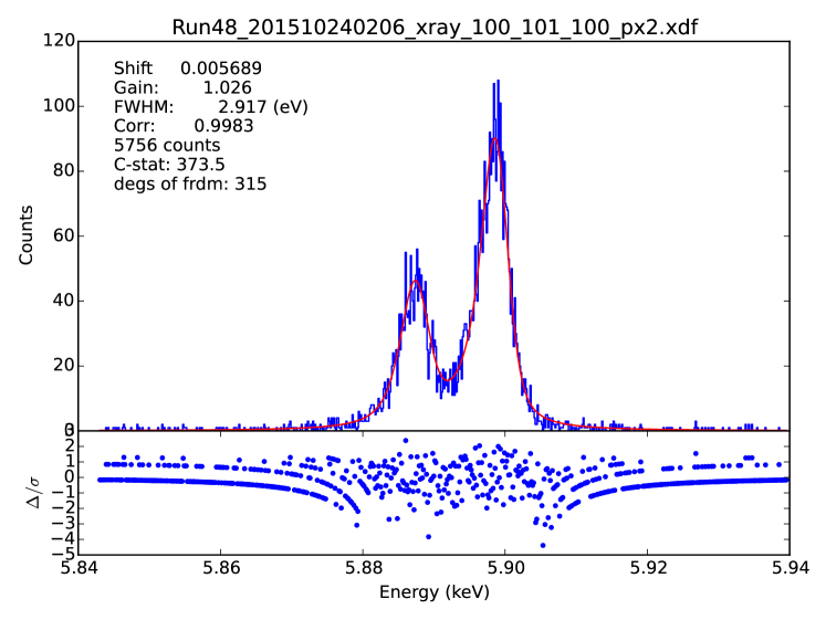
Figure 30: Correlation between the first two PCA components in frequency domain.

Figure 31: Fit of the instrumental resolution on the Mn-K_α line on the frequency domain PCA analysis. The instrumental resolution obtained shows a great improvement with respect to the time domain analysis (fig. 27) on the same data.

5 CONCLUSIONS

We performed PCA analysis on simulated data, both in time and frequency domain to study instrumental effects, and applied this analysis on real data from a multi pixel array obtained via frequency domain multiplexing. We conclude the following:

• Different instrumental effects can be recognized in the different PCA components obtained

• The relative importance of the different components in PCA analysis offers diagnostics on the possibility to separate different instrumental effects from photon energy

• PCA clearly shows that analysis in the frequency domain directly eliminates the problems with sampling phase and offers to obtain better energy resolution in a more efficient way

References

- [1] Barret, D., den Herder, J. W., Piro, L., Ravera, L., Den Hartog, R., Macculi, C., Barcons, X., Page, M., Paltani, S., Rauw, G., Wilms, J., Ceballos, M., Duband, L., Gottardi, L., Lotti, S., de Plaa, J., Pointecouteau, E., Schmid, C., Akamatsu, H., Bagliani, D., Bandler, S., Barbera, M., Bastia, P., Biasotti, M., Branco, M., Camon, A., Cara, C., Cobo, B., Colasanti, L., Costa-Kramer, J. L., Corcione, L., Doriese, W., Duval, J. M., Fabrega, L., Gatti, F., de Gerone, M., Guttridge, P., Kelley, R., Kilbourne, C., van der Kuur, J., Mineo, T., Mitsuda, K., Natalucci, L., Ohashi, T., Peille, P., Perinati, E., Pigot, C., Pizzigoni, G., Pobes, C., Porter, F., Renotte, E., Sauvageot, J. L., Sciortino, S., Torrioli, G., Valenziano, L., Willingale, D., de Vries, C., and van Weers, H., “The Hot and Energetic Universe: The X-ray Integral Field Unit (X-IFU) for Athena+,” ArXiv e-prints (Aug. 2013).
- [2] Nandra, K., Barret, D., Barcons, X., Fabian, A., den Herder, J.-W., Piro, L., Watson, M., Adami, C., Aird, J., Afonso, J. M., and et al., “The Hot and Energetic Universe: A White Paper presenting the science theme motivating the Athena+ mission,” ArXiv e-prints (June 2013).
- [3] den Hartog, R., Beyer, J., Boersma, D., Bruijn, M., Gottardi, L., Hoevers, H., Hou, R., Kiviranta, M., de Korte, P., van der Kuur, J., et al., “Frequency domain multiplexed readout of tes detector arrays with baseband feedback,” IEEE Transactions on Applied Superconductivity 21, 289–293 (2011).
- [4] Szymkowiak, A., Kelley, R., Moseley, S., and Stahle, C., “Signal processing for microcalorimeters,” Journal of Low Temperature Physics 93(3-4), 281–285 (1993).
- [5] Busch, S., Adams, J., Bandler, S., Chervenak, J., Eckart, M., Finkbeiner, F., Fixsen, D., Kelley, R., Kilbourne, C., Lee, S.-J., et al., “Progress towards improved analysis of tes x-ray data using principal component analysis,” Journal of Low Temperature Physics , 1–7 (2015).
- [6] Hölzer, G., Fritsch, M., Deutsch, M., Härtwig, J., and Förster, E., “K 1, 2 and k 1, 3 x-ray emission lines of the 3 d transition metals,” Physical Review A 56(6), 4554 (1997).
- [7] Wheaton, W. A., Dunklee, A. L., Jacobsen, A. S., Ling, J. C., Mahoney, W. A., and Radocinski, R. G., “Multiparameter linear least-squares fitting to Poisson data one count at a time,” ApJ 438, 322–340 (Jan. 1995).
- [8] Cash, W., “Parameter estimation in astronomy through application of the likelihood ratio,” ApJ 228, 939–947 (Mar. 1979).