CGC/saturation approach: a new impact-parameter dependent model in the next-to-leading order of perturbative QCD.

Abstract

This paper is the first attempt to build CGC/saturation model based on the next-to-leading order corrections to linear and non-linear evolution in QCD. We assume that the renormalization scale is the saturation momentum and found that the scattering amplitude has geometric scaling behaviour deep in the saturation domain with the explicit formula of this behaviour at large $\tau=r^{2}Q^{2}_{s}$. We built a model that include this behaviour, as well as the ingredients that has been known: (i) the behaviour of the scattering amplitude in the vicinity of the saturation momentum, using the NLO BFKL kernel; (ii) the pre-asymptotic behaviour of $\ln\left(Q^{2}_{s}\left(Y\right)\right)$, as function of $Y$ and (iii) the impact parameter behaviour of the saturation momentum, which has exponential behaviour $\propto\exp\left(-\,m\,b\right)$ at large $b$. We demonstrated that the model is able to describe the experimental data for the deep inelastic structure function. Despite this, our model has difficulties that are related to the small value of the QCD coupling at $Q_{s}\left(Y_{0}\right)$ and the large values of the saturation momentum, which indicate the theoretical inconsistency of our description.

1 Introduction.

This paper is the next step (see Ref. CLP ) in our attempt to find an approach, based on Color Glass Condensate/saturation effective theory for high energy QCD (see Ref. KOLEB for a review), which includes the impact parameter dependance of the scattering amplitude. Unfortunately, at the moment, our efforts reduce to building a model which incorporates the main features of the solution of the CGC/saturation equations, and also contains a number of phenomenological parameters for the non-perutbative QCD description of the large impact parameter dependance of the scattering amplitude.

We are doomed to build models to introduce the main features of the CGC/saturation approach, since the CGC/saturation equations do not reproduce the correct behavior of the scattering amplitude at large impact parameters (see Ref. KW ; FIIM ). Such failure leads to the conclusion: we cannot trust the solution of the CGC/saturation equations, without the long distance non-perturbative corrections at large impact parameters.

Indeed, for the scattering of a dipole with size $r$, with the nucleus, the CGC/saturation equations JIMWLK ; BK (see Eq.2.6 in Ref. KLT ) can be rewritten for $N\left(r,Y,Q_{T}=0\right)=\int d^{2}b\,N\left(r,Y,b\right)$ using the natural assumption that $r\,\ll\,R_{A}$ , where $R_{A}$ is the size of the nucleus. $N\left(r,Y,Q_{T}=0\right)$ is the infrared safe observable in perturbative QCD and, hence, we can expect that non-perturbative corrections for it, will be small. The radius of the dipole increases with energy growth, but from high energy phenomenology we learned that this increase is of the order $\alpha^{\prime}_{I\!\!P}\,Y\ll R_{A}$ for $Y\leq 40$. Implicitly, we assume that the non-perturbative corrections change the power like increase with energy of the interaction radius, that follows from perturbative QCD KW ; FIIM , to a logarithmic one, we believe that this change does not lead to the violation of the CGC/saturation equations.

However, for the interaction with a proton, we do not even have this, rather weak, argument and for a hadron target we anticipate large corrections to the CGC/saturation equations . Real progress in theoretical understanding of confinement of quarks and gluon has not yet been made , and as a result, we do not know how to change the CGC/saturation equations to incorporate confinement. We have to build a model which includes both theoretical knowledge that stems from the CGC/saturation equations, and the phenomenological large $b$ behavior, which do not contradict theoretical restrictions FROI ; BRLE .

Numerous attempts have been made over the past two decades (see Refs. CLP ; SATMOD0 ; SATMOD1 ; BKL ; SATMOD2 ; IIM ; SATMOD3 ; SATMOD4 ; SATMOD5 ; SATMOD6 ; SATMOD7 ; SATMOD8 ; SATMOD9 ; SATMOD10 ; SATMOD11 ; SATMOD12 ; SATMOD13 ; SATMOD14 ; SATMOD15 ; SATMOD16 ; SATMOD17 ) to build such models. Therefore, we clarify, in the introduction, the aspects of our model which are different.

The main difference of his paper from others, is that we use the nonlinear Balitsky-Kovchegov(BK) equation in the next-to-leading order (NLO) of perturbative QCD, that has been proven in Ref. NLOBK1 ; NLOBK2 ; NLOBK3 . The form of BK equation in the NLO shows that we can apply the method, suggested in Ref. LETU , for determining the behavior of the solution to BK equation deep inside the saturation region. This behavior in the NLO is given in this paper. It shows geometric scaling behaviour as in the leading order of perturbative QCD, for the renormalization scale which is equal to the saturation momentum $Q_{s}$.

We only introduce the non-perturbative impact parameter behavior in the saturation momentum, accordingly to the spirit of the geometric scaling behavior of the scattering amplitude BALE ; GS , and to the semi-classical solution to the CGC/saturation equations BKL . Similar assumptions for the non-perturbative $b$-behavior of the scattering amplitude, is typical for most models on the market (see Refs. SATMOD5 ; SATMOD6 ; SATMOD7 ; SATMOD8 ; SATMOD9 ; SATMOD12 ; SATMOD17 ). In the choice of the $b$ behavior we follow the procedure, suggested in Ref. CLP :

$$Q^{2}_{s}\left(b,Y\right)\,\propto\,\left(S\left(b,m\right)\right)^{\frac{1}{\bar{\gamma}}}$$ (1.1)

where $S\left(b\right)$ is the Fourier image of $S\left(Q_{T}\right)=1/\left(1+\frac{Q^{2}_{T}}{m^{2}}\right)^{2}$ and the value of $\bar{\gamma}$ we will discuss below. Such $b$ dependance results in the large $b$-dependence of the scattering amplitude, in the vicinity of the saturation scale which is proportional to $\exp\left(-mb\right)$ at $b\gg 1/m$, in accordance of the Froissart theorem FROI . In addition, we reproduce the large $Q_{T}$ dependence of this amplitude proportional to $Q^{-4}_{T}$ which follows from the perturbative QCD calculation BRLE .

In building our model we follow the strategy, suggested in Ref. IIM , which consists of matching the behavior of the scattering dipole amplitude deep in the saturation domain, that is found using the method of Ref. LETU , and the behavior of the scattering amplitude in the vicinity of the saturation scale KOLEB ; IIML ; MUT . In this paper, we follow the procedure of Ref. CLP ; CLM which allows us to combine the exact form of the solution inside the saturation domain and in the vicinity of the saturation scale. In Refs. SATMOD0 ; SATMOD1 ; BKL ; SATMOD2 ; IIM ; SATMOD3 ; SATMOD4 ; SATMOD5 ; SATMOD6 ; SATMOD7 ; SATMOD8 ; SATMOD9 ; SATMOD10 ; SATMOD11 ; SATMOD12 ; SATMOD13 ; SATMOD14 ; SATMOD15 ; SATMOD16 ; SATMOD17 only the characteristic behavior of the solution but not the exact form for it, was used.

We find the behavior of the amplitude in the vicinity of the saturation scale, using the NLO corrections to the BFKL Pomeron, calculated in Ref. BFKLNLO and the re-summation, suggested in Ref. SALAM . Such behavior has been discussed in Refs. T ; KMRS . In searching the parameters of the amplitude we use the procedure , suggested in Ref. KMRS , for full NLO kernel SALAM as it has been explored in Ref. T .

2 Theoretical input

2.1 General formula

The general formula for deep inelastic processes takes the form (see Fig. 1 and Ref. KOLEB for the review and references therein)

$$N\left(Q,Y;b\right)\,\,=\,\,\int\frac{d^{2}r}{4\,\pi}\int^{1}_{0}dz\,|\Psi_{\gamma^{*}}\left(Q,r,z\right)|^{2}\,N\left(r,Y;b\right)$$ (2.2)

where $Y\,=\,\ln\left(1/x_{Bj}\right)$ and $x_{Bj}$ is the Bjorken $x$. $z$ is the fraction of energy carried by quark. $Q$ is the photon virtuality. $b$ denotes the impact parameter of the scattering amplitude.

Eq. (2.2) splits the calculation of the scattering amplitude into two stages: calculation of the wave functions, and estimates of the dipole scattering amplitude.

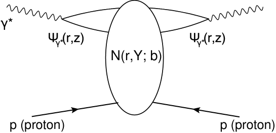
Figure 1: The graphic representation of Eq. (2.2) for the scattering amplitude. $Y=\ln\left(1/x_{Bj}\right)$ and $r$ is the size of the interacting dipole. $z$ denotes the fraction of energy that is carried by one quark. $b$ denotes the impact parameter of the scattering amplitude

2.2 Saturation momentum in the NLO

It is well known that the energy dependance of the saturation momentum can be found from the solution of the linear BFKL equation GLR ; BALE ; IIML ; MUT ; PEMU . In the leading order BFKL the saturation momentum $Q_{s}$ at large values of rapidity has the following form

$$Q^{2}_{s}\,\,\propto\,\,e^{\lambda Y}~{}~{}~{}~{}~{}\mbox{where}~{}~{}~{}\lambda\,\,=\,\,\bar{\alpha}_{S}\frac{\chi\left(\gamma_{cr}\right)}{1-\gamma_{cr}}~{}~{}~{}~{}\mbox{and}~{}~{}~{}\chi^{LO}\left(\gamma\right)\,=\,2\,\psi\left(1\right)\,-\,\psi\left(\gamma\right)\,-\,\psi\left(1-\gamma\right)$$ (2.3)

where $\psi\left(z\right)$ is the digamma function. $\gamma_{cr}$ is the solution of the equation

$$\frac{\chi\left(\gamma_{cr}\right)}{1-\gamma_{cr}}\,\,=\,\Big{|}\frac{d\chi\left(\gamma_{cr}\right)}{d\gamma_{cr}}\Big{|}$$ (2.4)

In the NLO, the spectrum of the BFKL equation has been found in Ref. BFKLNLO and it has the following form:

$$\omega\left(\gamma\right)\,\,=\,\,\bar{\alpha}_{S}\,\chi^{LO}\left(\gamma\right)\,\,+\,\,\bar{\alpha}_{S}^{2}\,\chi^{NLO}\left(\gamma\right)$$ (2.5)

The explicit form of $\chi^{NLO}\left(\gamma\right)$ is given in Ref. BFKLNLO (see Appendix 1). However, $\chi^{NLO}\left(\gamma\right)$ turns out to be singular at $\gamma\to 1$, $\chi^{NLO}\left(\gamma\right)\,\propto\,1/(1-\gamma)^{3}$. Such singularities indicate that we have to calculate higher order corrections to obtain a reliable result. The procedure to re-sum high order corrections is suggested in Ref. SALAM . The resulting spectrum of the BFKL equation in the NLO, can be found from the solution of the following equation SALAM ; T

$$\omega\,=\,\bar{\alpha}_{S}\left(\chi_{0}\left(\omega,\gamma\right)\,+\,\omega\,\frac{\chi_{1}\left(\omega,\gamma\right)}{\chi_{0}\left(\omega,\gamma\right)}\right)$$ (2.6)

where

$$\chi_{0}\left(\omega,\gamma\right)\,\,=\,\,\chi^{LO}\left(\gamma\right)\,-\,\frac{1}{1\,-\,\gamma}\,+\,\frac{1}{1\,-\,\gamma\,+\,\omega}$$ (2.7)

and

$$\chi_{1}\left(\omega,\gamma\right)\,\,=$$ (2.8)

$$\,\,\chi^{NLO}\left(\gamma\right)\,+\,F\left(\frac{1}{1-\gamma}\,-\,\frac{1}{1\,-\,\gamma\,+\,\omega}\right)\,+\,\frac{A_{T}\left(\omega\right)\,-\,A_{T}\left(0\right)}{\gamma^{2}}\,+\,\frac{A_{T}\left(\omega\right)-b}{\left(1\,-\,\gamma\,+\,\omega\right)^{2}}\,-\,\frac{A_{T}\left(0\right)-b}{\left(1\,-\,\gamma\right)^{2}}$$

Functions $\chi^{NLO}\left(\gamma\right)$ and $A_{T}\left(\omega\right)$ as well as the constants ($F$ and $b$) are presented in the Appendix A.

Denoting the solution of Eq. (2.6) $\omega^{NLO}\left(\gamma\right)$ we see that Eq. (2.4) for $\gamma_{cr}$ takes the form

$$\frac{\omega^{NLO}\left(\gamma_{cr}\right)}{1-\gamma_{cr}}\,\,=\,\Big{|}\frac{d\omega^{NLO}\left(\gamma_{cr}\right)}{d\gamma_{cr}}\Big{|}$$ (2.9)

This equation was firstly derived in Ref. GLR in the semi-classical approximation for the dipole scattering amplitude. In this approximation the amplitude appears as the wave packet and Eq. (2.9) is the condition that the phase velocity of this wave packet is equal to the group velocity. This condition determines the special line (critical line) which gives the saturation scale. In Refs. BALE ; KMRS Eq. (2.9) was derived beyond of the semi-classical approximation.

To find $\omega^{NLO}\left(\gamma_{cr}\right)$ and $\gamma_{cr}$ we do not need to solve Eq. (2.5)explicitly . We can solve the system of two equations:

$$\omega_{cr}\, = \,\bar{\alpha}_{S}\left(\chi_{0}\left(\omega_{cr},\gamma_{cr}\right)\,+\,\omega\,\frac{\chi_{1}\left(\omega_{cr},\gamma_{cr}\right)}{\chi_{0}\left(\omega_{cr},\gamma_{cr}\right)}\right)$$ (2.10)

$$\frac{\omega_{cr}}{1-\gamma_{cr}}\, = \,\bar{\alpha}_{S}\left(\chi_{0}\left(\omega_{cr},\gamma_{cr}\right)\,+\,\omega\,\frac{\chi_{1}\left(\omega_{cr},\gamma_{cr}\right)}{\chi_{0}\left(\omega_{cr},\gamma_{cr}\right)}\right)^{\prime}_{\gamma}\Bigg{/}\Bigg{(}1\,-\,\bar{\alpha}_{S}\left(\chi_{0}\left(\omega_{cr},\gamma_{cr}\right)\,+\,\omega\,\frac{\chi_{1}\left(\omega_{cr},\gamma_{cr}\right)}{\chi_{0}\left(\omega_{cr},\gamma_{cr}\right)}\right)^{\prime}_{\omega}\Bigg{)}$$

where $\omega_{cr}\equiv\omega^{NLO}\left(\gamma_{cr}\right)$. In Fig. 2 we plot the solution to this set of equations. One can see that both $\gamma_{cr}$ and $\lambda$ differ from the leading order estimates.

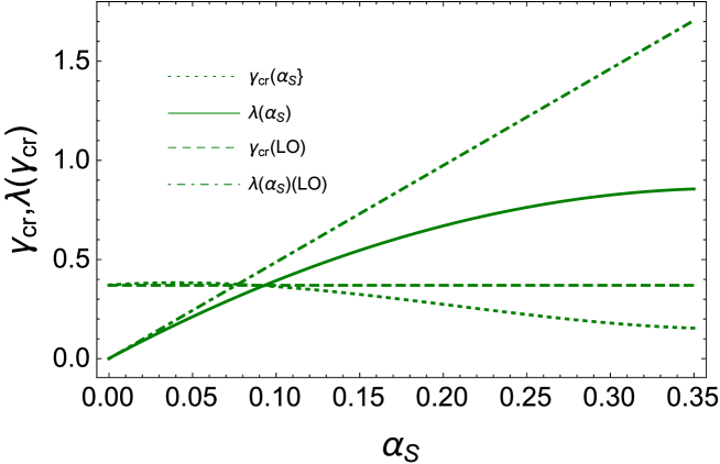
Figure 2: $\lambda(\gamma_{cr})$ and $\gamma_{cr}$ versus $\alpha_{S}$.

Fig. 3 shows the solution of Eq. (2.6) in the form $\gamma=\gamma\left(\omega\right)$. One can see that $\gamma=\gamma\left(\omega\right)\to 0$ at $\omega\to 1$. This property means that we have energy conservation in the NLO, while in the LO $\gamma\propto\bar{\alpha}_{S}\neq 0$ at $\omega\to 0$, indicating the energy violation of the order of $\bar{\alpha}_{S}$.

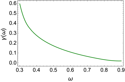
Figure 3: $\gamma$ versus $\omega$ for $\bar{\alpha}_{S}=0.15$.

The simple energy(rapidity) dependance of Eq. (2.3) only holds at large values of $Y$. The first two corrections lead to following expression

$$\ln\left(Q^{2}_{s}(Y)/Q^{2}_{s}(Y_{0},b)\right)\,=\,\lambda^{eff}\left(\bar{\alpha}_{S},Y,Y_{0}\right)\,\left(Y\,-\,Y_{0}\right)\,\,=$$ (2.11)

$$~{}~{}~{}~{}~{}~{}~{}~{}~{}~{}~{}~{}~{}\lambda(\gamma_{cr})\,(Y-Y_{0})\,\,-\,\,\frac{3}{2(1-\gamma_{cr})}\,\ln(Y/Y_{0})\,-\,\frac{3}{(1-\gamma_{cr})^{2}}\,\sqrt{\frac{2\,\pi}{\omega^{\prime\prime}(\gamma_{cr})}}\,\left(\frac{1}{\sqrt{Y}}\,-\,\frac{1}{\sqrt{Y_{0}}}\,\right)\,\,+\,\,{\cal O}\Big{(}\frac{1}{Y}\Big{)}$$

where $\omega^{\prime\prime}(\gamma_{cr})=d^{2}\omega(\gamma)/(d\gamma)^{2}$ at $\gamma=\gamma_{cr}$, the values of $\lambda\left(\gamma_{cr}\right)$ and $\gamma_{cr}$ have been discussed above. $Y_{0}$ is the value of rapidity from which we start the evolution. The first term was found in Ref. GLR , the second in Ref. MUT and the third in Ref. PEMU . In Fig. 4 $\ln\left(Q_{s}\left(b,Y\right)\Big{/}Q_{s}\left(b,Y=Y_{0}\right)\right)$ is plotted at different values of $\bar{\alpha}_{S}$ in the region of $Y\leq 12$ where the most experimental data are available. In this plot we take into account that the running QCD coupling has to be taken at scale $Q_{s}\left(Y\right)$ as we will argue in the next section, or in other words we use

$$\bar{\alpha}_{S}\left(Q_{s}\right)\,\,\frac{\bar{\alpha}_{S0}}{1\,+\,\bar{\alpha}_{S0}\,b\,\lambda_{cr}\,\left(Y-Y_{0}\right)}$$ (2.12)

where $\bar{\alpha}_{S0}$ =$\bar{\alpha}_{S}\left(Q_{0}\right)$ is the QCD coupling at the scale $Q_{0}=Q_{s}\left(Y=Y_{0}\right)$ (see Eq. (2.25)).

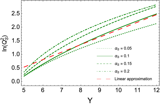
Figure 4: $\ln\left(Q_{s}\left(b,Y\right)\Big{/}Q_{s}\left(b,Y=Y_{0}\right)\right)$ versus $Y$ at different values of $\bar{\alpha}_{S}$.$Y_{0}=4.6$. For linear approximation we plot $0.7\,\lambda_{cr}\left(Y-Y_{0}\right)$ at $\bar{\alpha}_{S}=0.1$.

One can see that the corrections to $\ln\left(Q_{s}\left(b,Y\right)\Big{/}Q_{s}\left(b,Y=Y_{0}\right)\right)\,\,=\,\,\lambda_{cr}\,\left(Y-Y_{0}\right)$ are essential and they lead to $\lambda^{eff}\,\approx\,0.7\,\lambda_{cr}$. However, they turn out to be smaller than it was estimated in Ref.T , perhaps because the last term in Eq. (2.11) was not taken into account.

Eq. (2.11) shows that while we know the energy dependance theoretically, the value of $Q^{2}_{s}(Y_{0},b)$ is our phenomenological input which we will discuss below.

2.3 Scattering amplitude in the vicinity of the saturation scale

In the region where $r^{2}\,Q^{2}_{s}\left(Y,b\right)\,\approx\,\,1$ (in the vicinity of the saturation scale) the scattering amplitude has a well known behavior IIML ; MUT ; KOLEB

$$N\left(r,Y;b\right)\,\,=\,\,N_{0}\left(r^{2}\,Q^{2}_{s}\left(b\right)\right)^{1-\gamma_{cr}}$$ (2.13)

where $\gamma_{cr}$ is the solution to Eq. (2.10).

The amplitude of Eq. (2.13) shows a geometric scaling behavior as a function of one variable $\tau=r^{2}\,Q^{2}_{s}\left(b\right)$. Such behavior is proved inside the saturation region BALE ; LETU where $\tau\,\geq\,1$. However, it actually holds outside of the saturation region for $\tau\,\leq\,1$ IIML . In Ref. IIML it is shown that the first corrections due to a violation of the geometric scaling behavior, can be taken into account by replacing $1-\gamma_{cr}$ in Eq. (2.13) by the following expression

$$1\,-\,\gamma_{cr}\,\,\to\,\,1\,-\,\gamma_{cr}\,\,-\,\,\frac{1}{2\,\kappa\,\lambda\,Y}\,\ln\ \left(r^{2}\,Q^{2}_{s}\left(b\right)\right)$$ (2.14)

where $\lambda=\bar{\alpha}_{S}\chi\left(\gamma_{cr}\right)/\left(1-\gamma_{cr}\right)$ and $\kappa\,=\,\chi^{\prime\prime}\left(\gamma_{cr}\right)/\chi^{\prime}\left(\gamma_{cr}\right)$.

2.4 The scattering amplitude deep inside the saturation region ($r^{2}\,Q^{2}\left(b,Y\right)\,\gg\,1$)

The non-linear Balitsky-Kovchegov equation has been derived in the NLO, and it takes the form NLOBK1 ; NLOBK2 ; NLOBK2

$$\frac{\mathrm{d}S_{12}}{\mathrm{d}Y}\!= \frac{\bar{\alpha}_{S}}{2\pi}\!\int\!\!\mathrm{d}^{2}x_{3}\frac{x_{12}^{2}}{x_{13}^{2}x_{23}^{2}}\Bigg{\{}1\!+\!\bar{\alpha}_{S}b\left(\ln x_{12}^{2}\mu^{2}\!-\!\frac{x_{13}^{2}\!-\!x_{23}^{2}}{x_{12}^{2}}\ln\frac{x_{13}^{2}}{x_{23}^{2}}\right)$$

$$+\bar{\alpha}_{S}\left(\frac{67}{36}\!-\!\frac{\pi^{2}}{12}\!-\!\frac{5}{18}\,\frac{N_{f}}{N_{c}}\!-\!\frac{1}{2}\ln\frac{x_{13}^{2}}{x_{12}^{2}}\ln\frac{x_{23}^{2}}{x_{12}^{2}}\right)\Bigg{\}}\left(S_{13}S_{32}\!-\!S_{12}\right)$$

$$+\frac{\bar{\alpha}_{S}^{2}}{8\pi^{2}}\int\frac{\mathrm{d}^{2}x_{3}\,\mathrm{d}^{2}x_{4}}{x_{34}^{4}}\Bigg{\{}-2+\frac{x_{13}^{2}x_{24}^{2}+x_{14}^{2}x_{23}^{2}-4x_{12}^{2}x_{34}^{2}}{x_{13}^{2}x_{24}^{2}-x_{14}^{2}x_{23}^{2}}$$

$$\ln\frac{x_{13}^{2}x_{24}^{2}}{x_{14}^{2}x_{23}^{2}}+\frac{x_{12}^{2}x_{34}^{2}}{x_{13}^{2}x_{24}^{2}}\left(1+\frac{x_{12}^{2}x_{34}^{2}}{x_{13}^{2}x_{24}^{2}-x_{14}^{2}x_{23}^{2}}\right)\ln\frac{x_{13}^{2}x_{24}^{2}}{x_{14}^{2}x_{23}^{2}}\Bigg{\}}\left(S_{13}S_{34}S_{42}-S_{13}S_{32}\right)$$ (2.15)

in Eq. (2.4) $x_{ik}\,=\,\boldsymbol{x}_{i}\,-\,\boldsymbol{x}_{j}$, $\mu$ is the renormalization scale for the running QCD coupling and all other constants are defined in Appendix A. $S_{ij}$ is the S-matrix for scattering of a dipole of size $x_{ij}$, with the target.

One can see that in the region where $S_{ij}\to 0$, all terms except the first one, which is proportional to $S_{12}$, are small and can be neglected. In other words , in the region where $S_{12}\,\gg\,S_{13}\,S_{32}\,\gg\,S_{13}S_{34}S_{42}$ we can reduce Eq. (2.4) to the following linear equation LETU

$$\frac{\mathrm{d}S_{12}}{\mathrm{d}Y}\!=$$ (2.16)

$$-\,\,\frac{\bar{\alpha}_{S}}{2\pi}\!\int\!\!\mathrm{d}^{2}x_{3}\frac{x_{12}^{2}}{x_{13}^{2}x_{23}^{2}}\Bigg{\{}1\!+\!\bar{\alpha}_{S}b\left(\ln x_{12}^{2}\mu^{2}\!-\!\frac{x_{13}^{2}\!-\!x_{23}^{2}}{x_{12}^{2}}\ln\frac{x_{13}^{2}}{x_{23}^{2}}\right)+\bar{\alpha}_{S}\left(\frac{67}{36}\!-\!\frac{\pi^{2}}{12}\!-\!\frac{5}{18}\,\frac{N_{f}}{N_{c}}\!-\!\frac{1}{2}\ln\frac{x_{13}^{2}}{x_{12}^{2}}\ln\frac{x_{23}^{2}}{x_{12}^{2}}\right)\Bigg{\}}S_{12}$$

where $S_{12}\,\equiv\,1\,-\,N\left(x_{12},b,Y\right)$.

The integral over $x_{3}$ is taken in the Appendix B and Eq. (2.16) can be written in the form

$$\frac{\mathrm{d}\ln S_{12}}{\mathrm{d}Y}\!=\displaystyle{-\bar{\alpha}_{S}\left[1+\bar{\alpha}_{S}\,b\ln(\mu^{2}x_{12}^{2})+\bar{\alpha}_{S}\left(\frac{67}{36}-\frac{\pi^{2}}{12}-5\frac{N_{f}}{N_{c}}\right)\right]\ln(Q_{s}^{2}x_{12}^{2})+\frac{\bar{\alpha}_{S}^{2}b}{2}\ln^{2}Q_{s}^{2}x_{12}^{2}+\frac{\bar{\alpha}_{S}\zeta(3)}{16}}$$ (2.17)

In Eq. (2.17) almost all terms are function of $z\,=\,\ln\left(x^{2}_{12}\,Q^{2}_{s}\right)$, except the term $\bar{\alpha}_{S}\,b\ln(\mu^{2}x_{12}^{2})\ln(Q_{s}^{2}x_{12}^{2})$. Introducing the new renormalization point $Q^{2}_{s}$ instead of $\mu^{2}$ the equations reduces to the following one

$$\frac{\mathrm{d}\ln S_{12}}{\mathrm{d}Y}\! =$$

$$\displaystyle{-\bar{\alpha}_{S}\left(Q_{s}\right)\left[1+\frac{3}{2}\bar{\alpha}_{S}\left(Q_{s}\right)\,b\ln(Q_{s}^{2}x_{12}^{2})+\bar{\alpha}_{S}(Q_{s})\left(\frac{67}{36}-\frac{\pi^{2}}{12}-5\frac{N_{f}}{N_{c}}\right)\right]\ln(Q_{s}^{2}x_{12}^{2})+\frac{\bar{\alpha}_{S}(Q_{s})\zeta(3)}{16}}$$

Replacing $Y$ by $z\,=\,\ln\left(Q^{2}_{s}x^{2}_{12}\right)\,=\,\bar{\alpha}_{S}\left(Q_{s}\right)\,\varrho\,(Y-Y_{0})$ Eq. (2.4) takes the form

$$\frac{\mathrm{d}\ln S_{12}}{\mathrm{d}z}=\displaystyle{-\frac{1}{\varrho}\Bigg{(}\left[1+\frac{3}{2}\bar{\alpha}_{S}\left(Q_{s}\right)bz+\bar{\alpha}_{S}(Q_{s})\,\left(\frac{67}{36}-\frac{\pi^{2}}{12}-5\frac{N_{f}}{N_{c}}\right)\right]z+\frac{\zeta(3)}{16}}\Bigg{)}$$ (2.19)

Integration over $z$ leads to

$$\ln S_{12}=\displaystyle{-\frac{1}{2\,\varrho}\Bigg{(}\left[z+\bar{\alpha}_{S}\left(Q_{s}\right)bz^{2}+\bar{\alpha}_{S}(Q_{s})\,z\,\left(\frac{67}{36}-\frac{\pi^{2}}{12}-5\frac{N_{f}}{N_{c}}\right)\right]z+\frac{\zeta(3)}{8}}\,z\Bigg{)}$$ (2.20)

Eq. (2.20) shows a geometric scaling behavior, being a function of one variable $z$. However, this scaling behavior only holds, if we choose the renormalization scale $\mu=Q_{s}$.

Finally,

$$1-N\left(z\right)\, = \,e^{-{\cal Z}\left(z\right)}$$ (2.21)

with $${\cal Z}\left(z\right)\,=\,\frac{1}{2\,\varrho}\,\Bigg{(}\left[z+\bar{\alpha}_{S}\left(Q_{s}\right)bz^{2}+\bar{\alpha}_{S}(Q_{s})\,z\,\left(\frac{67}{36}-\frac{\pi^{2}}{12}-5\frac{N_{f}}{N_{c}}\right)\right]z-\,\frac{\zeta(3)}{8}\,z\Bigg{)}$$

where we replace $\varrho$ by $\varrho\,=\,\lambda_{cr}\left(\bar{\alpha}_{S}\right)/\bar{\alpha}_{S}$.

2.5 Matching at $r^{2}\,Q^{2}\left(b,Y\right)\,=\,1$

In section 2.3 we saw that the amplitude in the vicinity of the saturation scale has a geometric scaling behavior ( see Eq. (2.13)) as well as the amplitude at $r^{2}Q^{2}_{s}\gg 1$, as has been shown in the previous section. The first observation is that we can match these two amplitude, only if we assume that the renormalization scale $\mu=Q_{s}$. Practically , it means that we have to replace $\bar{\alpha}_{S}$ in section 2.3 by $\bar{\alpha}_{S}\left(Q_{s}\right)$ . This generates an additional $Y$ dependence, diminishing the value of $\lambda_{cr}$ at large values of $Y$.

The general matching conditions have the form of two following equations at $z=z_{m}$: We match these two solution at $z=z_{m}$ where

$$N^{0<z\ll 1}\left(z=z_{m}\right)\,=\,N^{z\gg 1}\left(z=z_{m}\right);~{}~{}~{}~{}~{}~{}~{}~{}~{}~{}~{}\frac{dN^{0<z\ll 1}\left(z=z_{m}\right)}{dz_{m}}\,=\,\frac{dN^{z\gg 1}\left(z=z_{m}\right)}{dz_{m}};~{}$$ (2.22)

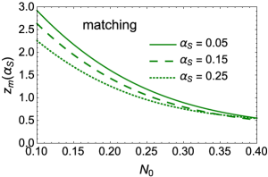
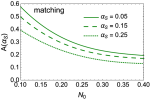
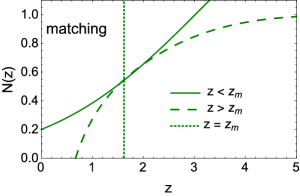
Fig. 5-a	Fig. 5-b	Fig. 5-c

Figure 5: Matching procedure: function $z_{m}\left(N_{0},\bar{\alpha}_{S}\right)$ (Fig. 5 -a), function $A\left(N_{0},\bar{\alpha}_{S}\right)$ (Fig. 5-b) and the example of the resulting function for $N_{0}=0.1$ and $\bar{\alpha}_{S}=0.15$ ( Fig. 5-c) .

These two equations determined the value of the amplitude and the point of matching. The additional restriction is that $z_{m}\ll 1$ , or, in other words $z_{m}$ should be in the vicinity of the saturation scale. A problem is that it is impossible to satisfy Eq. (2.22) without modifying the solution of Eq. (2.21). Most models in the past followed the suggestion of Ref. IIM and instead of Eq. (2.21), the modified solution

$$1\,-\,N\left(z\right)\,=\,e^{-C{\cal Z}\left(z\right)}$$ (2.23)

was introduced, in which the value of constant $C$ was determined by the matching conditions of Eq. (2.22). In Ref. CLM the correction to the asymptotic solution of Eq. (2.21) was found, which allows us to use the solution of Eq. (2.21) without an arbitrary unjustified constant $C$. This solution takes the form

$$N^{z\,\gg\,1}\left(z\right) \,=\, 1-2\,Ae^{-{\cal Z}}\,\,-\,A^{2}\,\frac{1}{{\cal Z}}\,e^{-2{\cal Z}}\,\,+\,\,{\cal O}\left(e^{-3{\cal Z}}\right)$$ (2.24)

$${\cal Z} = {\cal Z}\left({Eq.~{}(\ref{BKLT5})},z\to z-\frac{1}{2}A\sqrt{\varrho\,\pi/2}-2\psi(1)\right)$$

where $\psi(x)$ is the digamma function (see Ref. RY formula 8.360 - 8.367).

The second term in Eq. (2.24) is the solution given in Ref. LETU , in which the theoretically unknown constant $A$ is introduced, both as the coefficient in front, and as correction to the argument. The third term is the next order correction at large $z$. In Ref. CLM ; CLP it has been demonstrate that using Eq. (2.24), we can solve Eq. (2.22) and find $z_{m}$.

2.6 Impact parameter dependance of the saturation scale

So far we have introduced only one phenomenalogical parameter $N_{0}$: the value of the scattering amplitude at $r^{2}\,Q^{2}_{s}=1$. However, we need to specify the value of the saturation scale at $Y=Y_{0}$. It includes the value of the saturation scale and its dependence on the impact parameter $b$. Both can only be estimated in non-perturbative QCD. Due to the embryonic stage of our understanding of non-perturbative QCD contribution, we can only suggest a phenomenological parameterization.

For $Q_{s}\left(Y=Y_{0},b\right)$ we use the following expression

$$Q^{2}_{s}\left(Y=Y_{0},b\right)\,\,=\,\,Q^{2}_{0}\,S\left(b\right)\,\,=\,\,Q^{2}_{0}\,\left(m\,b\,K_{1}\left(m\,b\right)\right)^{1/(1-\gamma_{cr})}$$ (2.25)

The value of $m$ has to be find from the fitting of the experimental data. We expect that $m\approx 0.5\div 0.85\,GeV$ since $m=0.72\,GeV$ is the scale for the electromagnetic form factor of proton, while $m\approx 0.5\,GeV$ is the scale for so called gluon mass GLMASS.

We differ from other models in that Eq. (2.25) leads to $Q^{2}_{s}\left(Y=Y_{0},b\right)\,\xrightarrow{mb\,\gg\,1}\exp\left(-mb/(1-\gamma_{cr})\right)$, providing the correct large $b$ behavior of the scattering amplitude. It should be stressed that the exponential decrease at large $b$, follows from a general theoretical approach, based on analyticity and unitarity of the scattering amplitude (see FROI ). Therefore, $Q^{2}_{s}\left(Y=Y_{0},b\right)\,\propto\exp\left(-b^{2}/B\right)$ that was used in other models (see Refs. SATMOD5 ; SATMOD6 ; SATMOD7 ; SATMOD8 ; SATMOD9 ; SATMOD12 ; SATMOD17 ) are in the direct contradiction with theory. The behavior of the amplitude at large $b$ determines the energy dependance of the interaction radius, leading to $R\propto(1/m)Y$ for the exponential decrease, and $R\propto(1/m)\sqrt{Y}$ for the Gaussian $b$ dependance. Such a difference , leads to a fast increase of the scattering amplitude for our parameterization and it will effect the predictions at high energy.

Eq. (2.25) gives the amplitude in the vicinity of the saturation scale, which is proportional to $S\left(b\right)$ and generates the behavior $1/\left(1+\frac{Q^{2}_{T}}{m^{2}}\right)^{2}$, where $Q_{T}$ is the momentum transfer. At large $Q_{T}$ the amplitude in our parameterization is proportional ($A\propto 1/Q^{4}_{T}$) as it follows from the perturbative QCD calculation BRLE , but cannot be reproduced with the Gaussian distribution.

2.7 Wave functions

The wave function in the master equation (see Eq. (2.2)) is the main source of theoretical uncertainties: even in the case of deep inelastic processes, we can trust the wave function of perturbative QCD only, at rather large values of $Q^{2}\,\geq\,Q^{2}_{0}$ with $Q^{2}_{0}\approx 0.7GeV^{2}$ (see Ref. GLMTC ). The expression for $(\Psi^{*}\Psi)^{\gamma^{*}}\equiv\Psi_{\gamma^{*}}\left(Q,r,z\right)\,\Psi_{\gamma^{*}}\left(Q,r,z\right)$ is well known (see Ref. KOLEB and references therein)

$$(\Psi^{*}\Psi)_{T}^{\gamma^{*}} =\frac{2N_{c}}{\pi}\alpha_{\mathrm{em}}\sum_{f}e_{f}^{2}\left\{\left[z^{2}+(1-z)^{2}\right]\epsilon^{2}K_{1}^{2}(\epsilon r)+m_{f}^{2}K_{0}^{2}(\epsilon r)\right\},$$ (2.26)

$$(\Psi^{*}\Psi)_{L}^{\gamma^{*}} =\frac{8N_{c}}{\pi}\alpha_{\mathrm{em}}\sum_{f}e_{f}^{2}Q^{2}z^{2}(1-z)^{2}K_{0}^{2}(\epsilon r),$$ (2.27)

where T(L) denotes the polarization of the photon and $f$ is the flavours of the quarks. $\epsilon^{2}\,\,=\,\,m^{2}_{f}\,\,+\,\,Q^{2}z(1-z)$.

3 Fitting $F_{2}$ and values of the parameters

The most accurate experimental data available are for the deep inelastic structure function $F_{2}$ HERA1 , which we will attempt to fit using the model. As has been mentioned, we can trust our model in the restricted kinematic region, which we choose in the following way: $0.85\,GeV^{2}\leq Q^{2}\leq 60\,GeV^{2}$ and $x\,\leq\,0.01$. The lower limit of $Q^{2}$ stems from non-perturbative correction to the wave function of the virtual photon, while the upper limit originates from the restriction $x\,\leq\,0.01$. This restriction can be translated to the value of $Y_{0}$ in our theoretical formulae leading to $Y_{0}=4.6$. Actually we view $Y_{0}$ as the parameter of the fit (see Table 1).

$\bar{\alpha}_{S0}$	$N_{0}$	$Y_{0}$	m ($GeV$)	$Q^{2}_{0}$ ($GeV^{2}$)	$m_{u}$(MeV)	$m_{d}$(MeV)	$m_{s}$(MeV)	$m_{c}$(GeV)	$\chi^{2}/d.o.f.$
0.133	0.1075	3.77	0.83	3.0	2.3	4.8	95	1.4	183/153 =1.2
0.143	0.0915	3.73	0.67	2.6	140	140	140	1.4	242/153 = 1.58

Table 1: Parameters of the model. $\bar{\alpha}_{S0}$, $N_{0}$, $m$ and $Q^{2}_{0}$ are fitted parameters. The masses of quarks are chosen as they are shown in the table. Two sets are related to two choices of the quark masses: the current masses and the masses of light quarks are equal to $140\,MeV$ which is the typical infra-red cutoff in our approach.

Energy dependance of the saturation scale $Q_{s}$ and $\tau=r^{2}\,Q^{2}_{s}\left(b,Y\right)$ dependance of the scattering amplitude are determined by Eq. (2.11) and Eq. (2.22). One can see that both depend on $\bar{\alpha}_{S}\left(Q_{s}\right)$ for which we use Eq. (2.12). From this equation one can see that we have two fitting parameters: $\bar{\alpha}_{S0}$ and $Q^{2}_{0}$. In principle, $\bar{\alpha}_{S0}$ is the running QCD coupling at $Q^{2}=Q^{2}_{0}$, but we consider both $\bar{\alpha}_{S0}$ and $Q^{2}_{0}$ as independent fitting parameters, since we do not want to fix the value of $\Lambda_{\rm QCD}$. We have two dimensional parameters: $Q_{0}$, which determines the value of $Q_{s}^{2}$, and $m$ which determines its dependance on impact parameters $b$ ( see section 2.6). $N_{0}$ is the value of the scattering amplitude at $\tau=1$. In principle, the value of $N_{0}$ can be calculated using the linear evolution equation with the initial conditions. However, it depends on the phenomenological parameters of this initial condition. So we choose $N_{0}$ as a fitting parameter.

It is worth mentioning that $\lambda_{cr},\gamma_{cr}$ are not the fitting parameters as they are in the leading order models. We recall that

$$\ln\left(Q^{2}_{s}\left(b,Y\right)\Big{/}Q^{2}_{s}\left(b,Y=Y_{0}\right)\right)\,=\,d_{0}\left(\bar{\alpha}_{S}\right)\,Y\,\,+\,d_{1}\left(\bar{\alpha}_{S}\right)\ln\left(Y/Y_{0}\right)\,-\,d_{2}\left(\bar{\alpha}_{S}\right)\left(\frac{1}{\sqrt{Y}}\,-\,\frac{1}{\sqrt{Y_{0}}}\right)$$ (3.28)

where function $d_{i}$ are shown in Fig. 6. In Eq. (3.28) $Y=\ln\left(1/x\right)$, where $x$ is the Bjorken $x=Q^{2}/s$ for the deep inelastic scattering with the light quarks ( $Q$ is the photon virtuality and $s$ is the energy squared of collision). For the charm quark we consider $Y_{c}=\ln\left(1/x_{c}\right)$ with $x_{c}\,=\,(1+4\,m^{2}_{c}/Q^{2})\,x$.

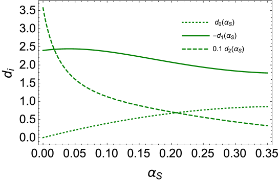
Figure 6: Function $d_{i}(\bar{\alpha}_{S})$ of Eq. (3.28) versus $\bar{\alpha}_{S}$.

We do not regard masses of the quark as fitting parameters and consider two sets of these masses. In the first set we take the current masses (see the first row of Table 1), and we consider this as the most reliable fit, based on the consistent theoretical approach. It should be mentioned that for the description of the interaction with $c$-quark we use $Y=\ln\left(1/x_{c}\right)$ with $x_{c}=x/(1+4\,m^{2}_{c}/Q^{2})$. We also make a fit putting all masses of light quarks (second row of Table 1) to be equal to 140 MeV. We view this mass as a typical infra-red cutoff that we introduce to take into account the unknown mechanism of confinement.

Table 1 gives the values of the fitting parameters, and Fig. 7 demonstrates the quality of the fit. One can see that we describe the data quite well but we have to admit that the quality of the fit is worse than in our model based on leading order QCD estimatesCLP , in which we fitted the value of $\lambda_{cr}$. $\chi^{2}/d.o.f=1.3$ in this fit against $\chi^{2}/d.o.f=1.15$ in the fit of Ref.CLP . However, the main complication of this model is that it gives rather a large value of $Q_{0}^{2}$ (see Fig. 8) which is in sharp contradiction to the value of the saturation momentum, from all other model description of the experimental dataCLP ; SATMOD0 ; SATMOD1 ; BKL ; SATMOD2 ; IIM ; SATMOD3 ; SATMOD4 ; SATMOD5 ; SATMOD6 ; SATMOD7 ; SATMOD8 ; SATMOD9 ; SATMOD10 ; SATMOD11 ; SATMOD12 ; SATMOD13 ; SATMOD14 ; SATMOD15 ; SATMOD16 ; SATMOD17 . The large value of $Q^{2}_{0}$ is in agreement with small values of $\bar{\alpha}_{S0}$, we note that $\bar{\alpha}_{S0}=0.28$ for $\Lambda_{\rm QCD}=158\,MeV$ instead of $\bar{\alpha}_{S0}=0.13$ from our fit.

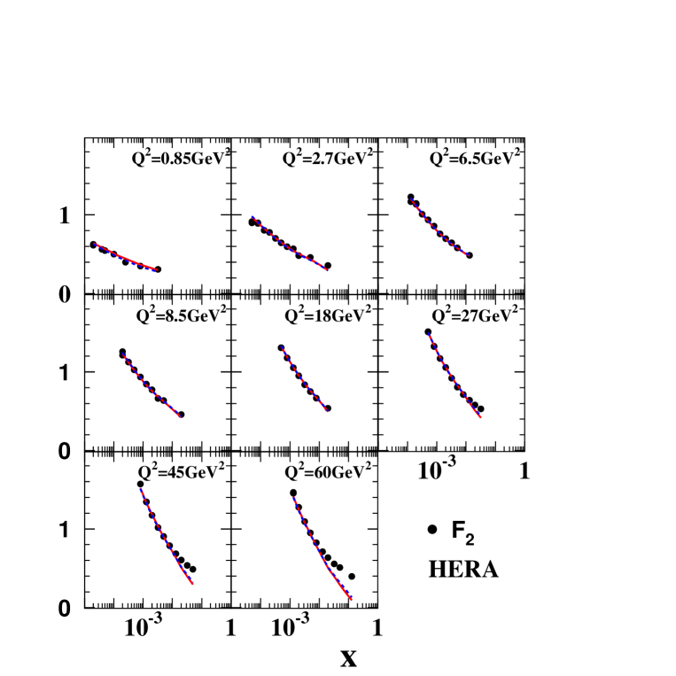
Figure 7: Our fit of $F_{2}$ with the values of parameters given by Table 1. The first set of parameters is shown in solid red curves while the second in blue dotted lines. The data is taken from Ref. HERA1 .

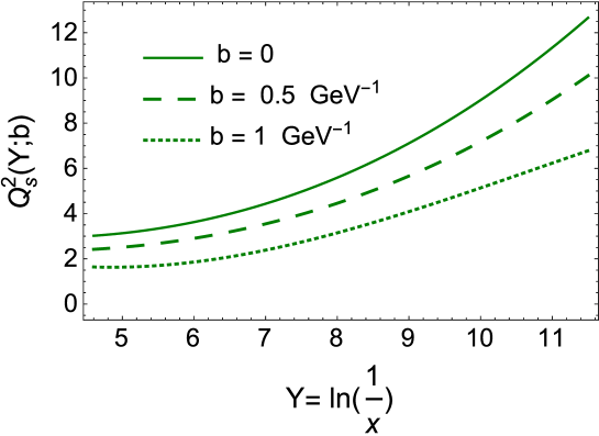
Figure 8: The value of the saturation momentum $Q^{2}_{s}\left(x,b\right)$ versus $x$ at fixed $b$ for the parameters given by Table 1.

The value of $m$ is larger than the typical mass in the electro-magnetic form factor of the proton, but we do not expect that it to be the same. Note that the decrease of $Q^{2}_{s}$ at large $b$ is proportional to $\exp\left(-\frac{m}{1-\gamma_{cr}}\,b\right)=\exp\left(-1.6\left(GeV^{-1}\right)\,b\right)$. On the other hand the behavior of amplitude on $b$ differs from the saturation scale. In Fig. 9 one can see that both the saturation, and the violation of the geometric scaling behavior influence the resulting b-dependence of scattering amplitude. Saturation flattens the $b$-dependence at small values of $b$, while the large $b$ behaviour shows a more rapid decrease than the $b$-dependence of the saturation scale (see Fig. 9).

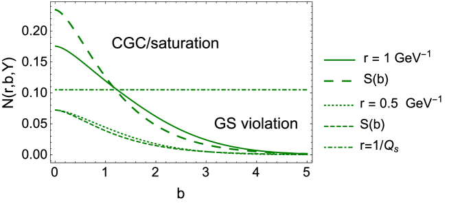
Figure 9: The $b$-dependence of the scattering amplitude for the parameters given by Table 1. $S\left(b\right)$ is given by Eq. (1.1).

It should be stressed that in the framework of our parametrization of the $b$-dependence of the saturation momentum, the scattering amplitude decreases as $\exp\left(-mb\right)$ while in all other models on the market it has a Gaussian behavior: $\exp\left(-m^{2}\,b^{2}\right)$.

Figure 10: The $x$-dependence of $F^{c\bar{c}}_{2}$ at small values of $Q^{2}\,<\,0.85\,GeV^{2}$ for the parameters given by Table 1. The red (upper) line corresponds to set 1(upper row of Table 1) while the blue one (low) is the description with set 2. The data are taken from Ref.HERAFL1 ; HERAFL2 .

Fig. 10 we present the comparison between our fit of $F_{2}$ with two sets of parameters at low values of $Q$. The set with large masses of quarks leads to a much better description illustrating the the non-perturbative corrections to the wave function of the virtual photon are essential at $Q^{2}\,<\,0.85\,GeV^{2}$.

$\mathbf{F_{2}^{c\bar{c}}}$ : The contribution of the $c\bar{c}$ pair to the deep inelastic structure function can be calculated with the same theoretical accuracy as the inclusive $F_{2}$. In Fig. 11 we compare the HERA data on $F^{cc}_{2}$ HERA2 with the theoretical predictions. One can see that the agreement is reasonable.

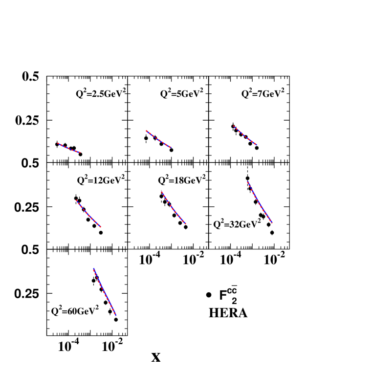
Figure 11: The $x$-dependence of $F^{c\bar{c}}_{2}$ at fixed values of $Q^{2}$: $0.85\,\leq\,Q^{2}\,\leq\,60\,GeV^{2}$ for the parameters given in Table 1. The data are taken from Ref. HERA2 .

$\mathbf{F_{L}}$ : $F_{L}$ can be calculated to the same accuracy as $F^{c\bar{c}}_{2}$, and the comparison with the scant data available HERAFL1 ; HERAFL2 is plotted in Fig. 12. Two sets produce the same quality of the descriptions since the values of $Q$ are rather large.

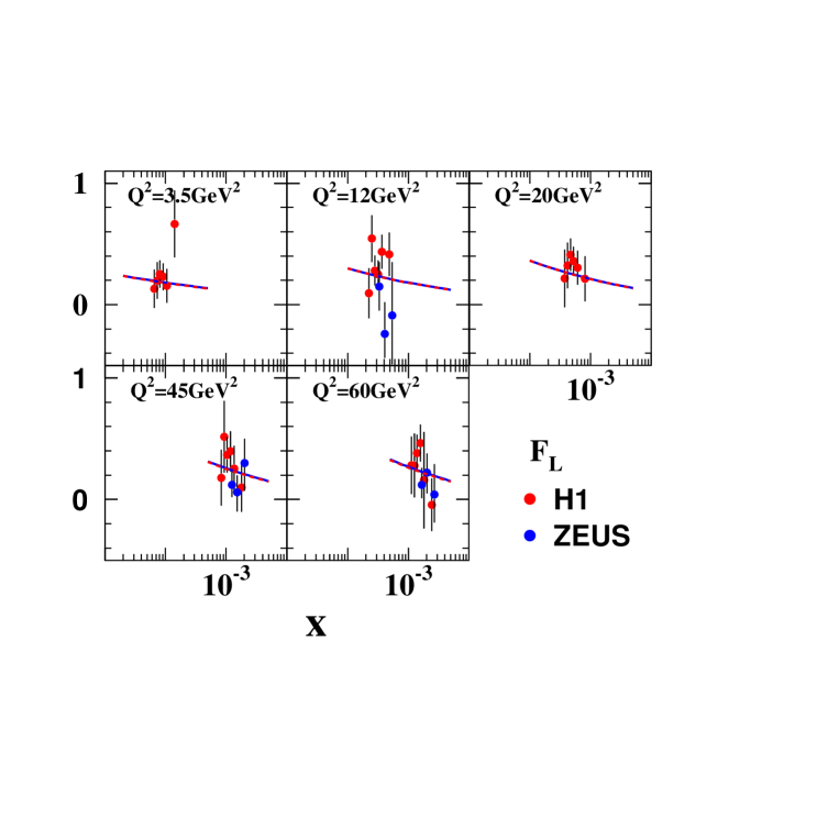
Figure 12: The $x$-dependence of $F_{L}$ at fixed values of $Q^{2}$: $0.85\,\leq\,Q^{2}\,\leq\,60\,GeV^{2}$ for the parameters given in Table 1. The red (blue) lines correspond to set 1 and set 2 fits. The data are taken from Ref. HERAFL2 .

4 Conclusions

In this paper we make the first attempt to include everything, that we have learned about the next-to-leading corrections of perturbative QCD, into the CGC/saturation model. In the paper we obtained two new theoretical results: (i) using the approach suggested in Ref.LETU , we obtained asymptotic behaviour of the solution to the Balitsky - Kovchegov equation in the NLO of perturbative QCD NLOBK1 ; NLOBK2 ; NLOBK2 deep inside of the saturation domain; and (ii) the geometric scaling behaviour of the scattering amplitude, which holds only if $\tau=r^{2}\,Q_{s}^{2}\left(Y;b\right)$ is determined in pQCD with the renormalization scale $Q_{s}\left(Y;b\right)$.

In the model we include several known ingredients: (i) the behaviour of the scattering amplitude in the vicinity of the saturation momentum, using the NLO BFKL kernel; (ii) the pre-asymptotic behaviour of $\ln\left(Q^{2}_{s}\left(Y\right)\right)$ as function of $Y$ and (iii) the impact parameter behaviour of the saturation momentum which has exponential behaviour $\propto\exp\left(-\,m\,b\right)$ at large $b$.

In comparison with the models on the market SATMOD0 ; SATMOD1 ; BKL ; SATMOD2 ; IIM ; SATMOD3 ; SATMOD4 ; SATMOD5 ; SATMOD6 ; SATMOD7 ; SATMOD8 ; SATMOD9 ; SATMOD10 ; SATMOD11 ; SATMOD12 ; SATMOD13 ; SATMOD14 ; SATMOD15 ; SATMOD16 ; SATMOD17 , we add the NLO corrections both deep in the saturation domain and in the vicinity of the saturation scale, as well as two crucial ingredients follow Ref.CLP : the correct solution to the non-linear (BK) equation BK in the saturation region, and impact parameter distribution that leads to exponential decrease of the saturation momentum at large impact parameters and to power-like decrease at large transfer momentum that follows from perturbative QCD.BRLE .

In spite of the fact that we describe the experimental data fairly we are aware that our description is worse than in the CGC/saturation models based on the leading order QCD approach. The main difficulties are related to the small value of the QCD coupling at $Q_{s}\left(Y_{0}\right)$, and the large values of the saturation momentum, which show the theoretical inconsistency of our description.

We cannot avoid the main assumption that the non-perturbative $b$ dependence is absorbed in the impact parameter behaviour of the saturation scale. However we are planning to improve the matching procedure given by Eq. (2.22), assuming the geometric scaling behaviour of the scattering amplitude as it stems from the form of $z$ dependence at large $z$ of the scattering amplitude found in this paper.

5 Acknowledgements

We thank our colleagues at Tel Aviv university and UTFSM for encouraging discussions. Our special thanks go to Asher Gotsman, Alex Kovner and Misha Lublinsky for elucidating discussions on the subject of this paper. This research was supported by the BSF grant 2012124, by Proyecto Basal FB 0821(Chile) , Fondecyt (Chile) grants 1130549 and 1140842, CONICYT grant PIA ACT1406 and by DGIP/USM grant 11.15.41.

Appendix A Resumed kernel of the NLO BFKL equation

For completeness of presentation we collect in this appendix all formulae for the NLO kernel of the BFKL equation, BFKLNLO resumed accordingly to the procedure, suggested in Ref. SALAM .

$$\chi^{NLO}\left(f\right)\, = \,-\frac{1}{4}\Bigg{(}2b\left(\chi^{\prime}(f)+\chi(f)^{2}\right)+\chi^{\prime\prime}(f)-\left(\frac{67}{9}-\frac{\pi^{2}}{3}-\frac{10}{9}\right)\chi(f)$$

$$+ \frac{\pi^{2}\cos(\pi f)\left(\frac{(3f(1-f)+2)\left(\frac{N_{f}}{N_{c}^{3}}+1\right)}{(3-2f)(2f+1)}+3\right)}{(1-2f)\sin^{2}(\pi f)}+4\phi(f)-\frac{\pi^{3}}{\sin(\pi f)}-6\zeta(3)\Bigg{)}$$

$$- \frac{1}{2}\chi(f)\chi^{\prime}(f)+\frac{\chi(f)}{(1-f)^{2}}$$ (A.30)

$$\phi(f)\, = \,\sum_{n=1}^{\infty}(-1)^{n}\left(\frac{\psi(-f+n+2)-\psi(1)}{(-f+n+1)^{2}}+\frac{\psi(f+n+1)-\psi(1)}{(f+n)^{2}}\right)$$ (A.31)

$$A_{GG}\left(\omega\right) = b-\frac{1}{\omega+1}+\frac{1}{\omega+2}-\frac{1}{\omega+3}-\left(\psi(\omega+2)-\psi(1)\right)$$

$$A_{QG}\left(\omega\right) = \frac{N_{f}}{N_{c}+2}\,\left(-\frac{2}{\omega+2}+\frac{2}{\omega+3}+\frac{1}{\omega+1}\right)$$

$$AA\left(\omega\right)\, = A_{GG}(\omega)+\frac{C_{f}}{N_{c}}\,A_{QG}(\omega)$$ (A.32)

$$b\,=\,\frac{11N_{c}\,-\,2N_{f}}{12\,N_{c}};~{}~{}~{}~{}C_{F}\,=\,\frac{N^{2}_{c}-1}{2\,N_{c}};~{}~{}~{}F=\frac{N_{f}}{6\,N_{c}}\left(\frac{5}{3}+\frac{13}{6N^{2}_{c}}\right);$$

$$\bar{\alpha}_{S}\left(p^{2}\right)\,\,=\,\,\frac{1}{b\,\ln\left(p^{2}/\Lambda_{QCD}^{2}\right)}\,\,=\,\,\frac{\bar{\alpha}_{S}(\mu)}{1\,+\,b\,\bar{\alpha}_{S}(\mu)\,\ln\left(p^{2}/\mu^{2}\right)}$$ (A.33)

In Ref. KMRS a very elegant form of $\chi_{1}\left(\omega,\gamma\right)$i was suggested which coincides with Eq. (2.6) to within $7\%$. The equation for $\omega$ takes the form

$$\omega\,=\,\bar{\alpha}_{S}\left(1-\omega\right)\left(\frac{1}{f}+\frac{1}{1-f+\omega}\,+\,\underbrace{\left(2\psi(1)-\psi\left(2-f\right)-\psi\left(1+f\right)\right)}_{\mbox{ high twist contributions}}\right)$$ (A.34)

One can see that $\gamma(\omega)\to 0$ when $\omega\to 1$ as follows from energy conservation.

In Fig. 13 we plot the values of $\lambda_{cr}$ and $\gamma_{cr}$ for the full kernel of Eq. (2.6) and for the simplified kernel of Eq. (A.34) suggested in Ref. KMRS . One can see that in spite of the fact that the simplified kernel coincides with the full one to within $7\%$, the difference in $\lambda_{cr}$ and in $\gamma_{cr}$ are much larger.

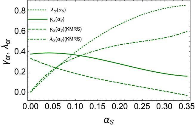
Figure 13: $\lambda(\gamma_{cr})$ and $\gamma_{cr}$ versus $\alpha_{S}$ for the full NLO kernel of Eq. (2.6) and for the kernel of Eq. (A.34).

Appendix B Calculation of integrals for the solution in the saturation region

In this appendix we take the integral of Eq. (2.16), which has the form

$$\frac{dS_{12}}{dY}=-\frac{\bar{\alpha}_{S}}{2\pi}K(Q_{s,}x_{12})\,S_{12}$$ (B.35)

where

$$K(Q_{s},x_{12})=$$ (B.36)

$$\int d^{2}x_{3}\frac{x^{2}_{12}}{x^{2}_{13}x^{2}_{23}}\left[1+\bar{\alpha}_{S}b\left(\ln(\mu^{2}x^{2}_{12})-\frac{x^{2}_{13}-x^{2}_{23}}{x^{2}_{12}}\ln\frac{x^{2}_{13}}{x^{2}_{23}}\right)+\bar{\alpha}_{S}\left(\frac{67}{36}-\frac{\pi^{2}}{12}-\frac{5}{18}\frac{N_{f}}{N_{c}}-\frac{1}{2}\ln\frac{x_{13}^{2}}{x_{12}^{2}}\ln\frac{x_{23}^{2}}{x_{12}^{2}}\right)\right]$$

Introducing the following notations

$$\begin{array}[]{rcl}I_{1}&=&\displaystyle{\int d^{2}x_{3}\frac{x^{2}_{12}}{x^{2}_{13}x^{2}_{23}}\left[1+\bar{\alpha}_{S}b\ln(\mu^{2}x^{2}_{12})+\bar{\alpha}_{S}\left(\frac{67}{36}-\frac{\pi^{2}}{12}-\frac{5}{18}\frac{N_{f}}{N_{c}}\right)\right]}\\ I_{2}&=&\displaystyle{\bar{\alpha}_{S}b\int d^{2}x_{3}\frac{x^{2}_{12}}{x^{2}_{13}x^{2}_{23}}\left[\frac{x^{2}_{23}-x^{2}_{13}}{x^{2}_{12}}\ln\left(\frac{x_{13}}{x_{23}}\right)\right]}\\ I_{3}&=&\displaystyle{-\frac{\bar{\alpha}_{S}}{2}\int d^{2}z_{3}\frac{x^{2}_{12}}{x^{2}_{13}x^{2}_{23}}\ln\frac{x_{13}^{2}}{x_{12}^{2}}\ln\frac{x_{23}^{2}}{x_{12}^{2}}}\end{array}$$

we have

$$K(Q_{s}z_{12})=I_{1}+I_{2}+I_{3}$$

Using the symmetry of the integrand with respect to $x_{13}\leftrightarrow x_{32}$ we obtain

$$\begin{array}[]{rcl}I_{2}&=&\displaystyle{\alpha\beta\int d^{2}x_{3}\frac{1}{x^{2}_{13}}\ln\left(\frac{x_{13}}{x_{23}}\right)-\bar{\alpha}_{S}b\int d^{2}x_{3}\frac{1}{x^{2}_{23}}\ln\left(\frac{x_{13}}{x_{23}}\right)}\\ &=&\displaystyle{\alpha\beta\int d^{2}x_{3}\frac{1}{x^{2}_{13}}\ln\left(\frac{x_{13}}{x_{23}}\right)+\bar{\alpha}_{S}b\int d^{2}x_{3}\frac{1}{x^{2}_{23}}\ln\left(\frac{x_{23}}{x_{13}}\right)}\\ &=&\displaystyle{\alpha\beta\int d^{2}x_{13}\frac{1}{x^{2}_{13}}\ln\left(\frac{x_{13}}{x_{23}}\right)+\bar{\alpha}_{S}b\int d^{2}x_{23}\frac{1}{x^{2}_{23}}\ln\left(\frac{x_{23}}{x_{13}}\right)}=\displaystyle{2\alpha\beta\int d^{2}x_{13}\frac{1}{x^{2}_{13}}\ln\left(\frac{x_{13}}{x_{23}}\right)}\end{array}$$ (B.37)

$I_{i}$ in polar coordinates take the form

$$\begin{array}[]{rcl}I_{1}&=&\displaystyle{\frac{1}{2}\int_{r_{0}^{2}}^{r_{1}^{2}}\frac{dr^{2}}{r^{2}}\int_{0}^{2\pi}\frac{1}{1+r^{2}-2r\cos\theta}d\theta\left[1+\bar{\alpha}_{S}b\ln(\mu^{2}x^{2}_{12})+\bar{\alpha}_{S}\left(\frac{67}{36}-\frac{\pi^{2}}{12}-\frac{5}{18}\frac{N_{f}}{N_{c}}\right)\right]};\\ \\ I_{2}&=&\displaystyle{\bar{\alpha}_{S}b\int_{r_{0}^{2}}^{r_{1}^{2}}\frac{dr^{2}}{r^{2}}\int_{0}^{2\pi}\ln\left(\frac{r^{2}}{1+r^{2}-2r\cos\theta}\right)d\theta};\\ I_{3}&=&\displaystyle{-\frac{\bar{\alpha}_{S}}{4}\int_{r_{0}^{2}}^{r_{1}^{2}}\frac{dr^{2}}{r^{2}}\int_{0}^{2\pi}\frac{1}{1+r^{2}-2r\cos\theta}\ln(r^{2})\ln(1+r^{2}-2r\cos\theta)d\theta}\end{array}$$ (B.38)

where $r^{2}=x^{2}_{13}/x^{2}_{12}$, $r_{0}^{2}=1/Q_{s}^{2}z_{12}^{2}$ and $r^{2}_{1}=1-1/Q_{s}^{2}z_{12}^{2}$. We use the following representations to take integral over the angle (see Ref. RY formulae 1.448, 1.511,3.613):

$$\begin{array}[]{rcl}\displaystyle{\int_{0}^{2\pi}\frac{\cos(n\theta)}{1+r^{2}-2r\cos\theta}d\theta}&=&\displaystyle{\frac{\Gamma(n+1)2\pi}{\Gamma(1)n!}r^{n}\ _{2}F_{1}(1,n+1;n+1,r^{2})=2\pi\frac{r^{n}}{1-r^{2}}}\\ \ln(1+r^{2}-2r\cos\theta)&=&-2\displaystyle{\sum_{n=1}^{\infty}\frac{\cos(n\theta)}{n}r^{n}};~{}~{}~{}~{}~{}~{}~{}~{}\ln(1-r^{2})=\displaystyle{-\sum_{n=1}^{\infty}\frac{r^{2n}}{n}}\end{array}$$ (B.39)

Using (B.39) for $Q_{s}^{2}z_{12}^{2}\gg 1$ we obtain

$$\begin{array}[]{rcl}I_{1}&=&\displaystyle{\pi\int_{r_{0}^{2}}^{r_{1}^{2}}dr^{2}\frac{1}{r^{2}(1-r^{2})}\left[1+\bar{\alpha}_{S}b\ln(\mu^{2}x_{12}^{2})+\bar{\alpha}_{S}\left(\frac{67}{36}-\frac{\pi^{2}}{12}-5\frac{N_{f}}{N_{c}}\right)\right]}\\ \\ &=&\displaystyle{2\pi\left[1+\bar{\alpha}_{S}b\ln(\mu^{2}x_{12}^{2})+\bar{\alpha}_{S}\left(\frac{67}{36}-\frac{\pi^{2}}{12}-5\frac{N_{f}}{N_{c}}\right)\right]\ln(Q_{s}^{2}x_{12}^{2})}\\ I_{2}&=&\displaystyle{2\pi\bar{\alpha}_{S}b\int_{r_{0}^{2}}^{r_{1}^{2}}dr^{2}\frac{\ln r^{2}}{r^{2}}d\theta}\,=\,\displaystyle{-\pi\bar{\alpha}_{S}b\ln^{2}Q_{s}^{2}x_{12}^{2}}\\ I_{3}&=&\displaystyle{-\frac{\bar{\alpha}_{S}}{4}\int_{r_{0}^{2}}^{r_{1}^{2}}dr^{2}\frac{\ln(r^{2})}{r^{2}}\int_{0}^{2\pi}\frac{1}{1+r^{2}-2r\cos\theta}\ln(1+r^{2}-2r\cos\theta)d\theta}\\ \\ &=&\displaystyle{-\frac{\bar{\alpha}_{S}}{4}\int_{r_{0}^{2}}^{r_{1}^{2}}dr^{2}\frac{\ln(r^{2})}{r^{2}}(-2)\sum_{n=1}^{\infty}\frac{r^{n}}{n}\int_{0}^{2\pi}\frac{\cos\theta}{1+r^{2}-2r\cos\theta}d\theta}\\ \\ &=&\displaystyle{-\frac{\bar{\alpha}_{S}}{4}\int_{r_{0}^{2}}^{r_{1}^{2}}dr^{2}\frac{\ln(r^{2})}{r^{2}}(-2)\sum_{n=1}^{\infty}\frac{r^{n}}{n}\left(\frac{2\pi r^{n}}{1-r^{2}}\right)d\theta}\\ \\ &=&\displaystyle{-\frac{2\pi\bar{\alpha}_{S}}{2}\int_{r_{0}^{2}}^{r_{1}^{2}}dr^{2}\frac{\ln(r^{2})\ln(1-r^{2})}{r^{2}(1-r^{2})}d\theta}\,=\,\displaystyle{-\frac{2\pi}{16}\zeta(3)}\end{array}$$ (B.40)

Hence, we obtain the following expression

$$-\frac{\bar{\alpha}_{S}}{2\pi}K(Q_{s}z_{12}) =$$

$$\displaystyle{-\bar{\alpha}_{S}\left[1+\bar{\alpha}_{S}b\ln(\mu^{2}z_{12}^{2})+\bar{\alpha}_{S}\left(\frac{67}{36}-\frac{\pi^{2}}{12}-5\frac{N_{f}}{N_{c}}\right)\right]\ln(Q_{s}^{2}z_{12}^{2})+\frac{\bar{\alpha}_{S}^{2}\beta}{2}\ln^{2}Q_{s}^{2}z_{12}^{2}+\frac{\bar{\alpha}_{S}\zeta(3)}{16}}$$

which we have used in section 2.4.

References

- (1) C. Contreras, E. Levin and I. Potashnikova, arXiv:1508.02544 [hep-ph].
- (2) Yuri V Kovchegov and Eugene Levin, “ Quantum Choromodynamics at High Energies", Cambridge Monographs on Particle Physics, Nuclear Physics and Cosmology, Cambridge University Press, 2012 .
- (3) A. Kovner and U. A. Wiedemann, Phys. Rev. D 66, 051502 (2002) [hep-ph/0112140]; Phys. Rev. D 66, 034031 (2002) [hep-ph/0204277]; Phys. Lett. B 551, 311 (2003) [hep-ph/0207335].
- (4) E. Ferreiro, E. Iancu, K. Itakura and L. McLerran, Nucl. Phys. A 710, 373 (2002) [hep-ph/0206241].
- (5) J. Jalilian-Marian, A. Kovner, A. Leonidov and H. Weigert, Phys. Rev. D59, 014014 (1999), [arXiv:hep-ph/9706377]; Nucl. Phys. B504, 415 (1997), [arXiv:hep-ph/9701284]; J. Jalilian-Marian, A. Kovner and H. Weigert, Phys. Rev. D59, 014015 (1999), [arXiv:hep-ph/9709432]; A. Kovner, J. G. Milhano and H. Weigert, Phys. Rev. D62, 114005 (2000), [arXiv:hep-ph/0004014] ; E. Iancu, A. Leonidov and L. D. McLerran, Phys. Lett. B510, 133 (2001); [arXiv:hep-ph/0102009]; Nucl. Phys. A692, 583 (2001), [arXiv:hep-ph/0011241]; E. Ferreiro, E. Iancu, A. Leonidov and L. McLerran, Nucl. Phys. A703, 489 (2002), [arXiv:hep-ph/0109115]; H. Weigert, Nucl. Phys. A703, 823 (2002), [arXiv:hep-ph/0004044].
- (6) I. Balitsky, [arXiv:hep-ph/9509348]; Phys. Rev. D60, 014020 (1999) [arXiv:hep-ph/9812311]; Y. V. Kovchegov, Phys. Rev. D60, 034008 (1999), [arXiv:hep-ph/9901281].
- (7) A. Kormilitzin, E. Levin and S. Tapia, Nucl. Phys. A 872, 245 (2011) doi:10.1016/j.nuclphysa.2011.09.021 [arXiv:1106.3268 [hep-ph]].
-
(8)
M. Froissart,
Phys. Rev. 123 (1961) 1053;
A. Martin, “Scattering Theory: Unitarity, Analitysity and Crossing." Lecture Notes in Physics, Springer-Verlag, Berlin-Heidelberg-New-York, 1969. - (9) G. P. Lepage and S. J. Brodsky, Phys. Rev. Lett. 43 (1979) 545; Phys. Rev. Lett. 43 (1979) 1625.
- (10) K. J. Golec-Biernat and M. Wusthoff, Phys. Rev. D 60 (1999) 114023 [hep-ph/9903358]; Phys. Rev. D 59 (1998) 014017; [hep-ph/9807513].
- (11) J. Bartels, K. J. Golec-Biernat and H. Kowalski, Phys. Rev. D 66 (2002) 014001 [hep-ph/0203258].
- (12) S. Bondarenko, M. Kozlov and E. Levin, Nucl. Phys. A 727 (2003) 139 [hep-ph/0305150].
- (13) H. Kowalski and D. Teaney, Phys. Rev. D 68 (2003) 114005 [hep-ph/0304189].
- (14) E. Iancu, K. Itakura and S. Munier, Phys. Lett. B 590 (2004) 199 [hep-ph/0310338].
- (15) H. Kowalski, L. Motyka and G. Watt, Phys. Rev. D 74 (2006) 074016 [hep-ph/0606272].
- (16) H. Kowalski, T. Lappi and R. Venugopalan, Phys. Rev. Lett. 100 (2008) 022303 [arXiv:0705.3047 [hep-ph]].
- (17) H. Kowalski, T. Lappi, C. Marquet and R. Venugopalan, Phys. Rev. C 78 (2008) 045201 [arXiv:0805.4071 [hep-ph]].
- (18) G. Watt and H. Kowalski, Phys. Rev. D 78 (2008) 014016 [arXiv:0712.2670 [hep-ph]].
- (19) E. Levin and A. H. Rezaeian, Phys. Rev. D 82 (2010) 014022 [arXiv:1005.0631 [hep-ph]].
- (20) A. H. Rezaeian, Phys. Lett. B 718 (2013) 1058 [arXiv:1210.2385 [hep-ph]].
- (21) E. Levin and A. H. Rezaeian, Phys. Rev. D 83 (2011) 114001 [arXiv:1102.2385 [hep-ph]].
- (22) E. Levin and A. H. Rezaeian, Phys. Rev. D 82 (2010) 054003 [arXiv:1007.2430 [hep-ph]].
- (23) D. Boer, M. Diehl, R. Milner, R. Venugopalan, W. Vogelsang, D. Kaplan, H. Montgomery and S. Vigdor et al., arXiv:1108.1713 [nucl-th].
- (24) T. Lappi and H. Mantysaari, Phys. Rev. C 83 (2011) 065202 [arXiv:1011.1988 [hep-ph]].
- (25) T. Toll and T. Ullrich, Phys. Rev. C 87 (2013) 2, 024913 [arXiv:1211.3048 [hep-ph]].
- (26) P. Tribedy and R. Venugopalan, Nucl. Phys. A 850 (2011) 136 [Nucl. Phys. A 859 (2011) 185] [arXiv:1011.1895 [hep-ph]].
- (27) P. Tribedy and R. Venugopalan, Phys. Lett. B 710 (2012) 125 [Phys. Lett. B 718 (2013) 1154] [arXiv:1112.2445 [hep-ph]].
- (28) A. H. Rezaeian, M. Siddikov, M. Van de Klundert and R. Venugopalan, PoS DIS 2013 (2013) 060 [arXiv:1307.0165 [hep-ph]]; Phys. Rev. D 87 (2013) 3, 034002 [arXiv:1212.2974].
- (29) A. H. Rezaeian and I. Schmidt, Phys. Rev. D 88 (2013) 074016 [arXiv:1307.0825 [hep-ph]].
- (30) I. Balitsky, Phys. Rev. D 75 (2007) 014001, [hep-ph/0609105].
- (31) Y. V. Kovchegov and H. Weigert, Nucl. Phys. A 784 (2007) 188, [hep-ph/0609090].
- (32) I. Balitsky and G. A. Chirilli, Phys. Rev. D 77 (2008) 014019, [arXiv:0710.4330 [hep-ph]]; I. Balitsky and G. A. Chirilli, Nucl. Phys. B 822 (2009) 45 [arXiv:0903.5326 [hep-ph]]; Phys. Rev. D 88 (2013) 111501 [arXiv:1309.7644 [hep-ph]].
- (33) E. Levin and K. Tuchin, Nucl. Phys. B 573, 833 (2000) [hep-ph/9908317]; Nucl. Phys. A 691, 779 (2001) [hep-ph/0012167]; 693, 787 (2001) [hep-ph/0101275].
- (34) J. Bartels, E. Levin, Nucl. Phys. B387 (1992) 617-637.
- (35) A. M. Stasto, K. J. Golec-Biernat, J. Kwiecinski, Phys. Rev. Lett. 86 (2001) 596-599, [hep-ph/0007192]; L. McLerran, M. Praszalowicz, Acta Phys. Polon. B42 (2011) 99, [arXiv:1011.3403 [hep-ph]] B41 (2010) 1917-1926, [arXiv:1006.4293 [hep-ph]]; M. Praszalowicz, Acta Phys. Polon. B 42 (2011) 1557 [arXiv:1104.1777 [hep-ph]]; M. Praszalowicz and T. Stebel, JHEP 1303 (2013) 090 [arXiv:1211.5305 [hep-ph]]; L. McLerran, M. Praszalowicz and B. Schenke, Nucl. Phys. A 916 (2013) 210 [arXiv:1306.2350 [hep-ph]]; M. Praszalowicz, Phys. Lett. B 727 (2013) 461 [arXiv:1308.5911 [hep-ph]]; L. McLerran and M. Praszalowicz, Phys. Lett. B 741 (2015) 246 [arXiv:1407.6687 [hep-ph]].
- (36) C. Contreras, E. Levin and R. Meneses, JHEP 1410 (2014) 138 [arXiv:1406.1212 [hep-ph]].
- (37) E. Iancu, K. Itakura and L. McLerran, Nucl. Phys. A 708 (2002) 327 [hep-ph/0203137].
- (38) A. H. Mueller and D. N. Triantafyllopoulos, Nucl. Phys. B 640 (2002) 331 [hep-ph/0205167].
- (39) V. S. Fadin and L. N. Lipatov, Phys. Lett. B 429 (1998) 127 [hep-ph/9802290]; M. Ciafaloni and G. Camici, Phys. Lett. B 430 (1998) 349 [hep-ph/9803389].
- (40) G. P. Salam, JHEP 9807 (1998) 019 doi:10.1088/1126-6708/1998/07/019 [hep-ph/9806482]; M. Ciafaloni, D. Colferai and G. P. Salam, Phys. Rev. D 60 (1999) 114036 doi:10.1103/PhysRevD.60.114036 [hep-ph/9905566], M. Ciafaloni, D. Colferai, G. P. Salam and A. M. Stasto, Phys. Rev. D 68 (2003) 114003, [hep-ph/0307188].
- (41) D. N. Triantafyllopoulos, Nucl. Phys. B 648 (2003) 293 [hep-ph/0209121].
- (42) V. A. Khoze, A. D. Martin, M. G. Ryskin and W. J. Stirling, Phys. Rev. D 70 (2004) 074013 [hep-ph/0406135].
- (43) L. V. Gribov, E. M. Levin and M. G. Ryskin, Phys. Rep. 100 (1983) 1.
- (44) S. Munier and R. B. Peschanski, Phys. Rev. D 70 (2004) 077503 [hep-ph/0401215]; Phys. Rev. D 69 (2004) 034008 [arXiv:hep-ph/0310357]; Phys. Rev. Lett. 91 (2003) 232001 [arXiv:hep-ph/0309177].
- (45) I. Gradstein and I. Ryzhik, Table of Integrals, Series, and Products, Fifth Edition, Academic Press, London, 1994.
- (46) E. Gotsman, E. Levin, U. Maor and E. Naftali, Eur. Phys. J. C 14 (2000) 511 [hep-ph/0001080].
- (47) F. D. Aaron et al. [H1 and ZEUS Collaborations], JHEP 1001 (2010) 109 [arXiv:0911.0884 [hep-ex]].
- (48) H. Abramowicz et al. [H1 and ZEUS Collaborations], Eur. Phys. J. C 73 (2013) 2, 2311 [arXiv:1211.1182 [hep-ex]].
- (49) V. Andreev et al. [H1 Collaboration], Eur. Phys. J. C 74 (2014) 4, 2814 [arXiv:1312.4821 [hep-ex]]; F. D. Aaron et al. [H1 Collaboration], Phys. Lett. B 665 (2008) 139 [arXiv:0805.2809 [hep-ex]].
- (50) H. Abramowicz et al. [ZEUS Collaboration], Phys. Rev. D 90 (2014) 7, 072002 [arXiv:1404.6376 [hep-ex]]; S. Chekanov et al. [ZEUS Collaboration], Phys. Lett. B 682 (2009) 8 [arXiv:0904.1092 [hep-ex]].