The interior rotation of a sample of $\gamma$ Doradus stars from ensemble modelling of their gravity mode period spacings

CONTEXT Gamma Doradus stars (hereafter $\gamma$ Dor stars) are known to exhibit gravity- and/or gravito-intertial modes that probe the inner stellar region near the convective core boundary. The non-equidistant spacing of the pulsation periods is an observational signature of the stars’ evolution and current internal structure and is heavily influenced by rotation.
AIMS We aim to constrain the near-core rotation rates for a sample of $\gamma$ Dor stars, for which we have detected period spacing patterns.
METHODS We combined the asymptotic period spacing with the traditional approximation of stellar pulsation to fit the observed period spacing patterns using $\chi^{2}$-optimisation. The method was applied to the observed period spacing patterns of a sample of stars and used for ensemble modelling.
RESULTS For the majority of stars with an observed period spacing pattern we successfully determined the rotation rates and the asymptotic period spacing values, though the uncertainty margins on the latter were typically large. This also resulted directly in the identification of the modes corresponding with the detected pulsation frequencies, which for most stars were prograde dipole gravity and gravito-inertial modes. The majority of the observed retrograde modes were found to be Rossby modes. We further discuss the limitations of the method due to the neglect of the centrifugal force and the incomplete treatment of the Coriolis force.
CONCLUSION Despite its current limitations, the proposed methodology was successful to derive the rotation rates and to identify the modes from the observed period spacing patterns. It forms the first step towards detailed seismic modelling based on observed period spacing patterns of moderately to rapidly rotating $\gamma\,$Dor stars.

1 Introduction

Gamma Dor stars are early F- to late A-type stars (with $1.4\,M_{\odot}\lesssim M\lesssim 2.0\,M_{\odot}$) which exhibit non-radial gravity and/or gravito-inertial mode pulsations (e.g. Kaye et al. 1999). This places them directly within the transition region between low-mass stars with a convective envelope and intermediate-mass stars with a convective core, where the CNO-cycle becomes increasingly important relative to the pp-chain as the dominant hydrogen burning mechanism (e.g. Silva Aguirre et al. 2011). The pulsations in $\gamma$ Dor stars are excited by the flux blocking mechanism at the bottom of the convective envelope (Guzik et al. 2000; Dupret et al. 2005), though the $\kappa$ mechanism has been linked to $\gamma$ Dor type pulsations as well (Xiong et al. 2016). The oscillations predominantly trace the radiative region near the convective core boundary. As a result these pulsators are ideal to characterise the structure of the deep stellar interior.

As shown by Tassoul (1980), high order ($n\gg l$) gravity modes are asymptotically equidistant in period for non-rotating chemically homogeneous stars with a convective core and a radiative envelope. This study was further expanded upon by Miglio et al. (2008). The authors found characteristic dips to be present in the period spacing series when the influence of a chemical gradient is included in the analysis. The periodicity of the deviations is related to the location of the chemical gradient, while the amplitude of the dips was found to be indicative of the steepness of the gradient. Bouabid et al. (2013) further improved upon the study by including the effects of both diffusive mixing and rotation, which they introduced using the traditional approximation. The authors concluded that the mixing processes partially wash out the chemical gradients inside the star, resulting in a reduced amplitude for the dips in the spacing pattern. Stellar rotation introduces a shift in the pulsation frequencies, leading to a slope in the period spacing pattern. Zonal and prograde modes, as seen by an observer in an inertial frame of reference, were found to have a downward slope, while the pattern for the retrograde high order modes has an upward slope.

Over the past decade the observational study of pulsating stars has benefitted tremendously from several space-based photometric missions, such as MOST (Walker et al. 2003), CoRoT (Auvergne et al. 2009) and Kepler (Koch et al. 2010). While typically only a handful of modes could be resolved using ground-based data, the space missions have provided us with near-continuous high S/N observations of thousands of stars on a long time base, resulting in the accurate determination of dozens to hundreds of pulsation frequencies for many targets. In particular, this has proven to be invaluable for $\gamma$ Dor stars, as their gravity and/or gravito-inertial mode frequencies form a very dense spectrum in the range of 0.3 to 3 $\rm d^{-1}$. Period spacing patterns have now been detected for dozens of $\gamma$ Dor stars (e.g. Chapellier et al. 2012; Kurtz et al. 2014; Bedding et al. 2015; Saio et al. 2015; Keen et al. 2015; Van Reeth et al. 2015; Murphy et al. 2016).

In this study we focus on the period spacing patterns detected by Van Reeth et al. (2015) in a sample of 68 $\gamma$ Dor stars with spectroscopic characterisation and aim to derive the stars’ internal rotation rate and the asymptotic period spacing value of the series. This serves as a first step for future detailed analyses of differential rotation, similar to the studies which have previously been carried out in slow rotators among g-mode pulsators interpreted recently in terms of angular momentum transport by internal gravity waves (e.g., Triana et al. 2015; Rogers 2015). In this paper we present a grid of theoretical models, which we use as a starting point (Section 2), and explain our methodology to derive the rotation frequency (Section 3). The method is illustrated with applications on synthetic data (Section 4.1), a slowly rotating star with rotational splitting, KIC 9751996, and a fast rotator with a prograde and a retrograde period spacing series, KIC 12066947 (Section 4.2). We then analyse the sample as a whole (Section 4.3), before moving on to the discussion and plans for future in-depth modelling of individual targets (Section 5).

2 Grid of stellar models and pulsation frequencies

We first computed a rough grid of theoretical stellar models to gain further insight into the internal structure and properties of $\gamma$ Dor stars. To allow for a complete understanding, the models were purposely kept relatively simple. We did not include any rotational effects into the equilibrium models, allowing us to assume spherical symmetry and compute 1-dimensional models with the 1D MESA stellar evolution code (v7385; Paxton et al. 2011, 2013, 2015). The convection was treated using the mixing length theory with $\alpha_{\rm MLT}=1.8$ and the Ledoux criterion with $\alpha_{\rm sc}=0.01$. A single diffusive mixing coefficient was defined in the radiative region and fixed at a value of $1\,cm^{2}s^{-1}$. We used the solar metallicity values given by Asplund et al. (2009) and OPAL type I opacity tables (Rogers & Nayfonov 2002). The varying parameter values of the models in the grid are given in Table 1.

For each of the models in our grid we also computed the asymptotic period spacing

$$\Delta\Pi_{l}=\frac{\Pi_{0}}{\sqrt{l(l+1)}},$$ (1)

with

$$\Pi_{0}=2\pi^{2}\left(\int_{r_{1}}^{r_{2}}N\frac{\mathrm{d}r}{r}\right)^{-1},$$ (2)

as derived by Tassoul (1980) for high-order gravity modes. Here $l$ is the spherical degree of the pulsation mode, $r$ is the distance from the stellar center, $N$ is the Brunt-Väisälä frequency and the boundaries of the mode trapping region are marked by $r_{1}$ and $r_{2}$ (Aerts et al. 2010). While $\Delta\Pi_{l}$ is smaller for larger values of $l$ (Eq. 1), $\Delta\Pi_{l}$ also changes as the star evolves. We have therefore calculated the probability of observing different spacing values using the stellar ages in our grid models. As shown in Fig. 1, we typically expect $\Delta\Pi_{l}$ values on the order of 3100 $s$ and 1800 $s$ for $l=1$ and $l=2$ respectively, which in turn implies $\Pi_{0}$ is on the order of $4400\,s$. In addition, there are strong linear correlations for $\Delta\Pi_{l}$ between models with different values of $M$, $Z$, $X$, $f_{\rm ov}$ and $\alpha_{\rm ov}$, assuming a fixed hydrogen abundance $X_{c}$ in the convective core.

As shown by Bouabid et al. (2013) and as observed by Van Reeth et al. (2015), gravity-mode period spacing patterns are heavily influenced by rotation. We therefore introduced the influence of rotation on the pulsation periods using the traditional approximation (Eckart 1960; Lee & Saio 1987; Townsend 2005). In this framework the $\theta$-component of the rotation vector is ignored (Lee & Saio 1997) and it is assumed that the star is sufficiently slowly rotating, so the effects of the centrifugal force can be neglected. While this particular assumption may not always be applicable, gravity-modes and gravito-inertial modes are mostly sensitive to the stellar properties near the convective core, where the rotational deformation of the star remains limited. This is illustrated in Fig. 2, which shows both the Brunt-Väisälä frequency $N$ and the rotational kernel $K_{nl}$ for the lowest- and highest-order mode of the stellar model discussed in Sec. 4.1. Both functions correlate with the sensitivity of the pulsations to the different regions in the star and peak near the convective core boundary. The rotational kernel $K_{nl}$ specifically indicates the sensitivity of the pulsations to the local stellar rotation profile. Thus, the rotational frequencies deduced from pulsational properties throughout this paper correspond with the near-core interior rotation rates.

Ballot et al. (2012) showed that the traditional approximation continues to perform adequately if the spin parameter $|s|\leq 2$ (see Ballot et al. 2012, Fig. 2), with

$$s=\frac{2f_{\rm rot}}{f_{co}},$$ (3)

where $f_{\rm rot}$ ($=\Omega/2\pi$) and $f_{co}$ are the stellar rotation frequency and the pulsation frequency in the corotating frame respectively. Thanks to the assumptions made in the traditional approximation, the computational requirements for the effects of rotation are dramatically reduced. In this work, we used the traditional approximation module from the 1D pulsation code GYRE v4.3 (Townsend & Teitler 2013), and follow the approach described by Ballot et al. (2012) and Bouabid et al. (2013). These authors show that, within the traditional approximation, an asymptotic pulsation period series can be rewritten for a rotating star as

$$P_{nlm,co}=\frac{\Pi_{0}}{\sqrt{\lambda_{l,m,s}}}(n+\alpha_{g}),$$ (4)

where $P_{nlm,co}$ is the pulsation period of radial order $n$, spherical degree $l$ and azimuthal order $m$ in the corotating frame. In this paper, we adopt the convention that $m>0$ corresponds with prograde modes and $m<0$ with retrograde modes, respectively. In this equation, $\lambda_{l,m,s}$ is the eigenvalue of the Laplace tidal equation depending on $l$, $m$, and the spin parameter $s$, while the phase term $\alpha_{g}$ depends on the internal stellar properties at the boundaries of the pulsation mode cavity and can be taken to be 0.5 for stars with a convective core and a convective envelope, such as $\gamma$ Dor stars. In the limit of a non-rotating star, where $s=0$, this expression reduces to

$$P_{nl}=\frac{\Pi_{0}}{\sqrt{l(l+1)}}(n+\alpha_{g}),$$ (5)

in agreement with Eq. (1) and as derived by Tassoul (1980). For each of the models in our grid, we computed the $l=1$ and $l=2$ mode frequencies for radial orders ranging from 5 to 120.

parameter	begin	end	step size
mass $M$ [$M_{\odot}$]	1.4	2.0	0.05
metallicity $Z$	0.010	0.018	0.004
exp. core overshooting $f_{ov}$	0.001	0.03	0.0075
step core overshooting $\alpha_{ov}$	0.01	0.3	0.075
initial hydrogen abundance $X_{i}$	0.69	0.73	0.02

Table 1: The parameter values of the computed grid of 1170 MESA evolutionary tracks, consisting of some 900,000 models.

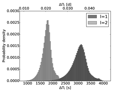
Figure 1: The distributions of the asymptotic period spacing values $\Delta\Pi_{l}$ for spherical degree $l=1$ and $2$, computed for the MESA evolution tracks with the input parameters provided in Table 1. For the computation of the distributions the ages and evolution rates of the stellar models were taken into account.

Figure 2: The Brunt-Väisälä frequency $N$ (top) and the rotational kernel $K_{nl}$ (bottom) for the lowest- and highest-order mode of the stellar model discussed in Sec. 4.1. The inset shows a zoom of $K_{nl}$. Both functions correlate with the sensitivity of the gravity-mode pulsations to the different regions inside the star.

3 Methodology

As we have discussed in the previous section, the influence of rotation on the pulsation frequencies depends on the values of both $l$ and $m$, while the asymptotic spacing $\Delta\Pi_{l}$ is dependent of the value of $l$ (Eq. 1). It is therefore necessary to have a pulsation mode identification if we wish to constrain the rotation profile of the observed star properly.

To derive a reliable estimate of the rotation rate of a $\gamma$ Dor star with one or more observed period spacing patterns, we consider all the possible combinations of $l$ and $m$-values for the mode identification of the GYRE pulsation frequencies computed for the MESA models in our grid. For each combination of (l,m), we compute the asymptotic spacing value $\Delta\Pi_{l}$, as expressed in Eq. (1) and subsequently correct it in the framework of the traditional approximation according to Eq. (5). This is illustrated graphically in Fig. 3. Because the application of a rotational frequency shift does not introduce dips into the period spacing patterns, we do not need to take them into account at this point. A uniform period spacing series is sufficient for our needs.

The pulsation frequencies in this series are then rotationally shifted using the traditional approximation, as described by Eq. 4 and assuming the star is rigidly rotating. The values of the pulsation periods in the inertial reference frame are then obtained by

$$P_{\rm inert}=\frac{1}{f_{co}+mf_{\rm rot}}.$$ (6)

This introduces a slope into the model spacing series, as shown in Fig. 3. The resulting pattern is subsequently fitted to the observed period spacing series using $\chi^{2}$-minimisation, optimising for the variables $\Delta\Pi_{l}$ and $f_{rot}$. Finally, we select the best solution for all studied $l$ and $m$ values, taking into account the theoretical expectations for the asymptotic spacing $\Delta\Pi_{l}$, as shown in Fig. 1 and derived from our model grid in Sec. 2. From this fit, we then obtain estimates for the rotation rate $f_{rot}$ and the asymptotic spacing $\Delta\Pi_{l}$, as well as a mode identification.

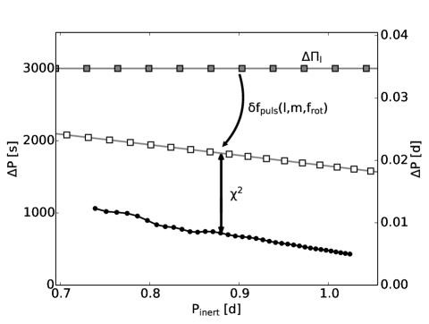
Figure 3: Illustration of our methodology to derive the rotation rate $f_{\rm rot}$ and asymptotic spacing $\Delta\Pi_{l}$ from an observed period spacing pattern (black dots). An equidistant spacing series (grey squares) is defined, rotationally shifted (white squares) and fitted to the observed pattern using $\chi^{2}$-minimisation, optimising for the variables $l$, $m$, $\Delta\Pi_{l}$ and $f_{rot}$.

4 Applications

4.1 Synthetic data

To illustrate our method we first analyse a simulated period spacing pattern. The simulated data were computed using the MESA and GYRE codes with the input values provided in Table 2, further taking ($l$,$m$) = (1,1). For the computation of the evolution track itself the influence of rotation was not taken into account. The rotation was only included in the GYRE computations using the traditional approximation module. The computed pattern is shown in Fig. 4 and the values of the pulsation periods are listed in the appendix in Table 4.

The results of our analysis are shown in Figs. 4 to 6. As we can see in Fig. 4 we fitted the simulated data nicely when we excluded the dips in the pattern from the analysis and assumed ($l$,$m$) = (1,1). However, similar good results were obtained when we treated the pulsations as (2,1)-modes or (2,2)-modes during our analysis, as illustrated in Fig. 5. In other words, we cannot obtain a clear mode identification if we base ourselves solely on the obtained $\chi^{2}$-values. This problem is solved when we look back to the expected values of the asymptotic spacing $\Delta\Pi_{l}$ for different values of $l$, which we previously showed in Fig. 1. It is clear that the found values for $\Delta\Pi_{l}$ are far too large for $l=2$. We can therefore safely identify the simulated data as (1,1)-modes, and obtain $f_{\rm rot}=0.664\pm 0.013\,d^{-1}$ and $\Delta\Pi_{l=1}=3020\pm 190\,s$.

It is important to exclude any significant dips in the period spacing structure from this analysis. In our technique, we do not take the influence of chemical gradients in the stellar interior into account. As shown by Miglio et al. (2008), these result in non-uniform deviations from the asymptotic spacing series. Because we can only observe a small part of a period spacing pattern, any non-uniform variations in the pattern will change the measured mean spacing and/or the measured slope of the pattern. This, in turn, will influence our analysis. By ignoring significant non-uniform variations in the period spacing structure, we limit their influence on the analysis, so that we obtain results which are correct within or on the order of $1\sigma$. For our simulated data set this is illustrated with the 2-dimensional $\chi^{2}$-distribution shown in Fig. 6. While we ignored the large dip in the period spacing structure (as seen in Fig. 4), the remaining non-uniform variations still impacted the analysis. As a result, there is a small offset between the input values of the data set and the 1$\sigma$-confidence interval for the obtained solution.

parameter	values
mass $M$ [$M_{\odot}$]	1.63
metallicity $Z$	0.016
initial hydrogen abundance $X_{i}$	0.71
mixing length parameter $\alpha_{MLT}$	1.8
step core overshooting $\alpha_{ov}$	0.18
mixing coefficient $D$ [$cm^{2}s^{-1}$]	0.8
$T_{\rm eff}$ [K]	7047
$\log g$ [dex]	4.34
$[M/H]$ [dex]	0.094
$v_{\rm eq}$ [km $\rm s^{-1}$]	69.38
$f_{\rm rot}$ [$\rm d^{-1}$]	0.674
$\Delta\Pi_{l=1}$ [$s$]	3186.5
central hydrogen abundance $X_{c}$	0.357

Table 2: The parameter values of the simulated period spacing pattern. Top: the input parameters of the MESA evolution track. Bottom: the parameters of the model for which the pulsation periods were computed.

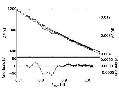
Figure 4: Top: the input period spacing pattern (black dots and grey triangles) with the best-fitting pattern (white squares) as obtained from the $\chi^{2}$-minimisation in Fig.6 assuming ($l$,$m$) = (1,1). The black part of the input patterns was used to determine $f_{rot}$ and $\Delta\Pi_{l}$, while the grey section was excluded. Bottom: the residuals of the fit.

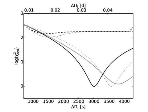
Figure 5: The best $\chi^{2}$-values for the synthetic data shown in Fig. 2 for each ($l,m$)-combination, as a function of the asymptotic spacing $\Delta\Pi_{l}$. The black and light grey lines correspond to $l=1$ and $l=2$ respectively, while the modes with $m=0$ are indicated with dashed lines, $m=1$ with full lines and $m=2$ with the dash-dotted line.

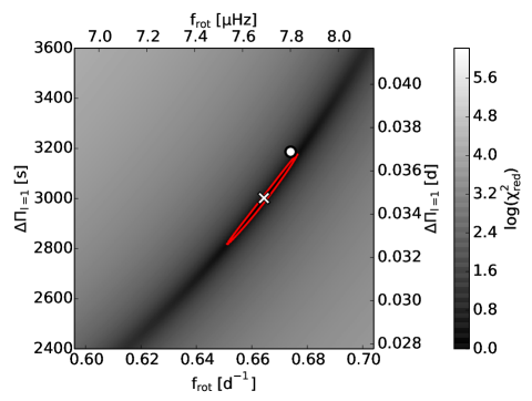
Figure 6: $\log(\chi^{2}_{\rm red})$ for the simulated period spacing series assuming $l=1$, as a function of the asymptotic period spacing $\Delta\Pi_{l}$ and the rotation rate $f_{rot}$. The white dot indicates the input values, while the white cross and the red boundary indicate the found solution and its 1$\sigma$-uncertainty margins respectively.

4.2 A slow and a fast rotator

In our sample we have one slowly rotating star, KIC 9751996, for which we detected period spacing series with rotational splitting, delivering immediately the $m$-values of the modes. In order to further validate our proposed methodology, we have applied it to KIC 9751996. In a first step, we only analysed the prograde period spacing pattern to test the reliability of our method. Assuming ($l$,$m$) = (1,1), this led us to find $f_{\rm rot}=0.07\pm 0.02\,d^{-1}$, which is shown in the top of Fig. 7. However, assuming $l=1,m=0$ for the treated series, we found $f_{\rm rot}=0.19\pm 0.03\,d^{-1}$ for a similar $\chi^{2}$ value. The challenge in this case is that the shift and the slope in the period spacing pattern are almost negligibly small compared to the non-uniform period spacing variations due to a chemical gradient. This was resolved when we fit the prograde, zonal and retrograde dipole modes simultaneously, as shown in Fig. 8. Not only did this allow us to formally identify the $(l,m,n)$-values of the modes, it also resulted in a much higher precision for the rotation rate $f_{\rm rot}=0.0696\pm 0.0008\,d^{-1}$ and the spacing $\Delta\Pi_{l=1}=3086\pm 6\,s$ (See Fig. 7). Interestingly, we have another indication for this derived rotation rate independently. Both in the series of the prograde modes and of the retrograde modes, we have a pulsation period which does not seem to follow the pattern, at values of 0.8 days and 0.9 days, respectively. These modes are likely trapped, which has influenced their pulsation period. When the periods of these retrograde and prograde modes are converted to their values in the corotating reference frame using the derived rotation rate, we find the pulsation periods are almost equal, which is consistent with the interpretation of trapped pulsation modes.

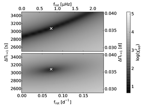
Figure 7: $\log(\chi^{2}_{\rm red})$ for the observed period spacing series of KIC 9751996, assuming $l=1$, as a function of the asymptotic period spacing $\Delta\Pi_{l}$ and the rotation rate $f_{rot}$. The white crosses indicate the optimal found solutions. Top: the $\chi^{2}$-distribution that we find by only analysing the detected prograde series. Bottom: the $\chi^{2}$-distribution obtained by fitting the prograde, zonal and retrograde spacing series simultaneously.

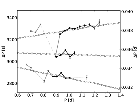
Figure 8: The observed period spacing patterns (black dots and grey triangles) for the retrograde (top), zonal (middle) and prograde (bottom) modes of KIC 9751996. The black parts of the input patterns were used to determine $f_{rot}$ and $\Delta\Pi_{l}$, while the grey sections were excluded. The white squares indicate the modes of the optimal model in the grid when all three series are fitted simultaneously.

Next we also analysed the period spacing patterns of KIC 12066947, a fast rotating star for which both a prograde and a retrograde period spacing series were detected. While we were able to fit the pattern of prograde modes to derive a rotation rate $f_{rot}$, the observed retrograde series presented us with a challenge. We found these to correspond with Rossby modes rather than “classical” gravity or gravito-inertial modes. Rossby modes can only occur in rotating stars and originate from the interaction between the stellar rotation and toroidal modes (e.g. Papaloizou & Pringle 1978; Townsend 2003b). Our identification of the retrograde modes as Rossby modes is illustrated in the top panel of Fig. 9, where we show the observed period spacing patterns for both the detected prograde and retrograde series, as well as the spacings predicted by the most suitable model in the grid, by assuming the values for $f_{rot}$ and $\Delta\Pi_{l}$ obtained by modelling the prograde series. For the calculation of the period series in the case of Rossby modes, $\Pi_{0}$ was derived from $\Delta\Pi_{l}$ using Eq. (1), and this value was subsequently filled into Eq. (4). The appropriate eigenvalues $\lambda$ were computed using the asymptotic approximation derived by Townsend (2003b), i.e. Eq. (37) in that study. This equation is valid when $\lambda\neq m^{2}$, as is the case here. The expected values of $\lambda$ for Rossby modes are three to four orders of magnitude smaller than for retrograde gravito-inertial modes, which allowed us to identify the observed pulsations. However, as Townsend (2003b) pointed out, the asymptotic approximation does not converge well to the numerical solution in the case of such modes. The possibility to compute Rossby modes has currently not yet been included in the publicly available version of GYRE. As a consequence, we could not do a reliable quantitative analysis of the retrograde series at this point and limited ourselves to the analysis of the prograde series to derive $f_{\rm rot}$. However, several qualitative arguments can be made in favour of Rossby modes as a correct identification. From the upward slope and the small average period spacing of the observed pattern, we derive that these modes are retrograde in the corotating frame with $|f_{co}|<f_{rot}$, which is completely in line with the theoretical expectations. Furthermore, the observed spin parameter values are larger for the retrograde than for the prograde modes, e.g., the values of the dominant modes of both series are $15.8\,\pm 0.4$ and $7.7\,\pm 0.1$, respectively. This indicates that in the corotating frame the pulsation frequencies of the retrograde modes are smaller than those of the prograde modes, which in turn can be explained by the small values of the eigenvalues $\lambda$. Finally, Townsend (2003b) also notes that, compared to the retrograde gravito-inertial modes, Rossby modes are less equatorially confined as the stellar rotation rate increases. As a result, the latter can be expected to be less influenced by the geometrical cancellation effects, though the effect is still present. For KIC 12066947, we find that the dominant prograde and Rossby modes are confined within equatorial bands with a width of 77.2° and 53.5° respectively.

For a fast rotating star such as KIC 12066947, we also have to take into acccount rotational deformation. The centrifugal force leads to a lower effective gravity at the equator than at the pole. This influences the Brunt-Väisälä frequency, which affects the pulsations. In the case of KIC 12066947, we could roughly estimate the deformation of the star, using equation A.6 from Maeder & Meynet (2000). In this analysis we evaluated the observed spectroscopic parameter values and asymptotic spacing $\Delta\Pi_{l}$ using the models in our MESA grid and took the best matching model ($M=1.5M_{\odot}$, $Z=0.014$, $X_{i}=0.69$, $X_{c}=0.452$, $\alpha_{\rm ov}=0.01$) as a guess for the stellar structure. We found that $f_{\rm rot}/f_{\rm rot,crit}=0.78$ and $R_{\rm pole}/R_{\rm eq}=0.88$. A two-dimensional treatment of the rotation is clearly needed to quantify the impact of the rotation on the modes, which will allow us to improve our constraints on $f_{\rm rot}$ and $\Delta\Pi_{l}$.

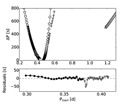
Figure 9: Top: The observed period spacing patterns (black dots and grey triangles) for the prograde (left) and retrograde (right) modes of KIC 12066947. The black part of the pattern was used to determine $f_{rot}$ and $\Delta\Pi_{l}$, while the grey section was excluded. The white squares indicate the model fit, assuming we are dealing with gravito-inertial modes and using the $f_{rot}$ and $\Delta\Pi_{l}$ values obtained from the analysis of the marked prograde series. The white diamonds indicate the model computed for Rossby waves using the same $f_{rot}$ and $\Delta\Pi_{l}$ values, assuming $m=-1$ and $k=-2$ in the k-based indexing scheme by Lee & Saio (1997). Bottom: The residuals of the fit to the prograde period spacing series.

4.3 Sample study

Subsequently, we also applied our methodology to the other stars in our sample. This led to the mode identification and the determination of the rotation rate $f_{\rm rot}$ for the period spacing series of 40 stars in our sample. Six additional sample stars only exhibit retrograde modes and fast rotation, and cannot be quantitatively analysed with our current methodology. In the case of the remaining four stars, the difference of the best $\chi^{2}$-value for different ($l$,$m$) combinations is too small, so no unique solution could be determined.

For the 40 stars which were successfully analysed, the results are listed in the appendix in Table LABEL:tab:param. The vast majority of the studied stars were found to exhibit prograde dipole modes. For fourteen targets in the sample we had detected multiple series. In principle, these are prime targets to look for differential rotation. However, for ten of them the second detected period spacing pattern corresponds to Rossby modes, for which we still need to develop a suitable computational tool to arrive at appropriate numerical values, as discussed in Section 4.2. For the remainder of this study, we assign the values of $f_{\rm rot}$ and $\Delta\Pi_{l}$ which we obtained from the prograde series to the retrograde series of the same star. Because formal mode identification of these retrograde pulsations is currently not possible, they are marked as “R” in Table LABEL:tab:param. For two other stars we have both a zonal and prograde dipole series, while for a third we have prograde dipole and quadrupole modes. Finally, KIC 9751996, the slowly rotating star we discussed in Sec. 4.2, is the only target for which we have a series of rotationally split multiplets. For each of these last four stars, we were able to use the multiple detected period spacing patterns to refine the obtained $f_{\rm rot}$ and $\Delta\Pi_{l}$.

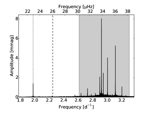
Figure 10: Part of the frequency spectrum of KIC 7365537. The light grey area shows the location of the pulsation modes which form the detected period spacing pattern of this star. The dashed line marks the value of the derived rotation frequency $f_{\rm rot}$, while the dotted line indicates the solitary high-amplitude mode which was found.

There are several stars for which a single high-amplitude mode was detected, which does not belong to a period spacing series and which differs from the rotation frequency. In Fig. 10 we show the frequency spectrum of KIC 7365537 as an example. For these modes the identification in Table LABEL:tab:param is marked “S”. Because our method can not be applied to these single modes, we again use the values of $f_{\rm rot}$ and $\Delta\Pi_{l}$ which were derived from the prograde series in the same star, in the subsequent analysis. The selection of series of modes in some stars versus the presence of single modes in others also tells us a great deal about their respective stellar structure. It has been suggested by Dziembowski & Pamyatnykh (1991) that such single high-amplitude modes could occur due to mode trapping effects. However, detailed theoretical modelling of each of these individual stars is required to confirm this.

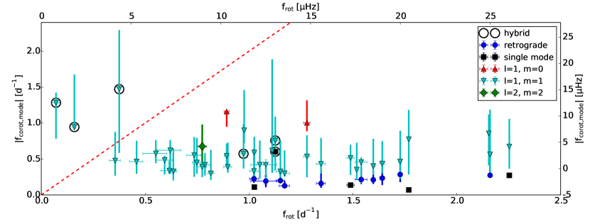
Figure 11: The dominant pulsation frequency $f_{dom,corot}$ in the corotating frame as a function of the rotation frequency $f_{rot}$ for the identified g-mode pulsations of 40 stars in the sample. The thick vertical lines indicate the full extent of the detected spacing series. The dashed red line marks where the pulsations pass from the superinertial regime (above the line) into the subinertial regime (below the line).

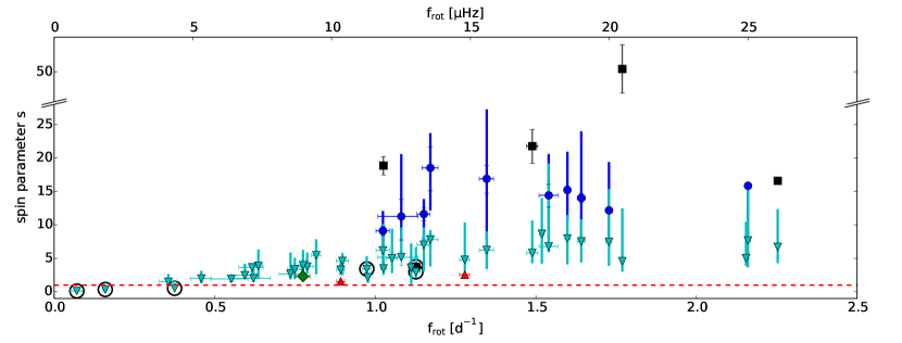
Figure 12: The absolute value of the spin parameter $s$ for the detected period spacing series of the stars in our sample, as a function of the rotation frequency $f_{rot}$. The dashed red line marks where the pulsations pass from the superinertial regime (below the line) into the subinertial regime (above the line). The used symbols are the same as in Fig. 11.

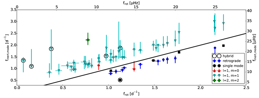
Figure 15: The dominant pulsation frequency $f_{dom,inert}$ in the inertial frame as a function of the rotation frequency $f_{rot}$ for the identified g-mode pulsations of 40 stars in the sample. The thick vertical lines indicate the full extent of the detected spacing series. The full black line indicates where $f_{\rm inert}$ is equal to $f_{\rm rot}$.

Fig. 11 illustrates the frequency $f_{\rm dom,corot}$ of the dominant mode of each detected series in the corotating frame with respect to the computed rotation frequency. An alternative version of Fig. 11 in the inertial reference frame is included in the appendix in Fig. 15. For the majority of the stars, we obtain similar values of $f_{\rm dom,corot}$ between 0.15 and 0.75 $\rm d^{-1}$. This can be linked to the convective flux blocking excitation mechanism. Dupret et al. (2005) and Bouabid et al. (2013) remarked that, in order for the mode excitation mechanism to be efficient, the thermal timescale $\tau_{th}$ at the bottom of the convective envelope has to be on the order of the pulsation periods in the corotating frame. From this information and the content of Fig. 11, we can then also derive that both the detected retrograde spacing series and single modes likely have azimuthal order $m=-1$, because only $|m|=1$ led to similar $f_{\rm dom,corot}$ values for the series of different stars. While these results are consistent, we note that the observed pulsation periods in the corotating frame are typically larger than the theoretical values computed by Bouabid et al. (2013). For the retrograde Rossby modes this can be linked to the correspondingly low eigenvalues $\lambda$ of the Laplace tidal equation. However, the same discrepancy is observed for the prograde modes as well, though to a lesser degree. This discrepancy may point towards limitations of the current theory of mode excitation in $\gamma$ Dor stars for moderate to fast rotators or may be caused by the limited applicability of the traditional approximation for these rotation rates. Further research on this topic is required.

In Fig. 12 we show the spin parameter $s$, as defined in Eq. (3) and listed in the last column of Table LABEL:tab:param, as a function of the measured rotation frequency $f_{\rm rot}$. The spin parameter $s$ is a measure of the impact of rotation on the pulsation frequency and is inversely proportional to the pulsation frequency $f_{\rm co}$ in the corotating frame. Once again, the Rossby modes (marked with dark blue dots) have small values for the eigenvalue $\lambda$. In addition, despite the fact that both prograde sectoral modes and Rossby modes are less easily confined in a band around the equator, the effect is still significant for these high values of $s$ (Townsend 2003b). This implies many of the stars in our sample are seen at moderate to high inclination angles. We further note that our observed values of $s$ are on average much larger than the values quoted in theoretical papers in the literature (e.g. Townsend 2003a; Ballot et al. 2012).

Fig. 13 offers a closer look at the three slowest rotating stars in our sample, one of which is KIC 9751996 already discussed in Sec. 4.2. These three stars have comparable properties. They are slow rotators, placing them in the superinertial regime, and they are hybrid $\gamma$ Dor/$\delta$ Sct pulsators. Each of them exhibits variability in the frequency range between 5 $\rm d^{-1}$ and 8 $\rm d^{-1}$. These striking similarities suggest there is a link between the stars’ low rotation rates and their hybrid properties, marking them as interesting targets for follow-up research.

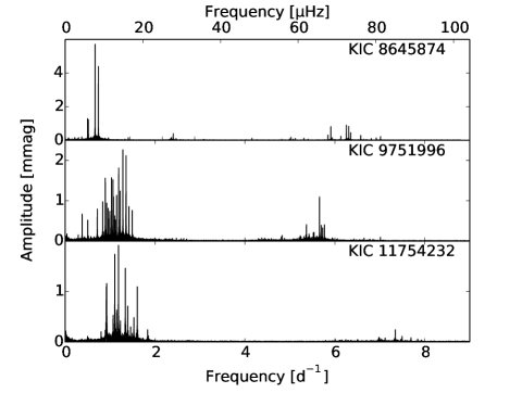
Figure 13: A section of the Fourier spectra of the three slowest rotating stars in our sample. These are our only stars in the superinertial regime, and all three are hybrid $\gamma$ Dor/$\delta$ Sct pulsators with variability between 5 $\rm d^{-1}$ and 8 $\rm d^{-1}$.

4.3.1 Statistical analysis

Finally, we also look for correlations between the parameter values of our stars, similar to the multivariate statistical analysis which was carried out by Van Reeth et al. (2015). In this work, we again use the spectroscopic fundamental parameter values obtained by Van Reeth et al. (2015) in our analysis. We also include the detected values of the variables $f_{\rm rot}$, $\Delta\Pi_{l}$, $R\sin\,i=v\sin\,i/f_{\rm rot}$ and the dominant pulsation frequency $f_{\rm dom}$ (both in the corotating and the inertial reference frame). For consistency, we limit ourselves to the parameter values derived from the identified prograde dipole mode series of 40 stars in the sample. The results of our multivariate statistical study are summarised in Table 3.

Most of the correlations presented previously by Van Reeth et al. (2015) were indicative of the strong relation between the observed gravity-mode pulsations and the stellar rotation. In retrospect, these can now be linked to the identification of most pulsations as prograde dipole gravity, gravito-inertial or retrograde Rossby modes with $|m|=1$. In particular, those previous results are echoed in our current work by the detected correlations between $f_{\rm rot}$ and $v\sin i$, and $f_{\rm rot}$ and $f_{\rm dom,inert}$. The strong correlation between $f_{\rm rot}$ and $v\sin i$ is illustrated in Fig. 14. The previously detected correlations between $v\sin i$ and the mean period spacing $\langle\Delta P\rangle$, the mean pulsation period $\langle P\rangle$ and the mean slope $\langle\frac{\mathrm{d}\Delta P}{\mathrm{d}P}\rangle$ of the observed series discussed in Van Reeth et al. (2015) are now also reflected in similar correlations with $f_{\rm rot}$. We do find a level of scatter in the relationship between these parameters and the rotation rate $f_{\rm rot}$, originating from the large variety of radial orders of the detected modes, the limited lengths of some of the observed series and from non-uniform variations in the period spacing patterns covered by our sample. Moreover, we have assumed a constant rotation rate throughout the stars to deduce $f_{\rm rot}$, which is simplistic compared to predictions based on numerical simulations (Rogers 2015). Allowing for a variety of non-uniform interior rotation profiles will likely complicate the correlations.

Van Reeth et al. (2015) also found a smaller contribution of $T_{\rm eff}$ to the multivariate correlation with $f_{\rm dom,inert}$ and $v\sin i$. While this contribution drops when we replace $v\sin i$ with $f_{\rm rot}$, there is a weak correlation between $T_{\rm eff}$ and $R\sin i$. Indeed, as a star ages, its temperature $T_{\rm eff}$ drops and its radius increases. A similar weak correlation was found between $f_{\rm rot}$ and $\log\,g$, indicating that as the star evolves and its radius increases, both the surface gravity and the rotation rate decrease. The correlation between $R\sin i$ and $\log\,g$ was not significant, likely due to the relatively large uncertainties.

In contrast, we did not find correlations between the asymptotic spacing $\Delta\Pi_{l}$ and any of the other parameters. The uncertainty margins on the value of $\Delta\Pi_{l}$ are likely too large for a proper correlation to be unravelled. Multivariate correlations were not detected either.

Table 3: Results of the linear regression analysis. We list the coefficients of the covariates for the different correlations as well as their $p$-values (obtained from a $t$-test) and $R^{2}$ values.

Explanatory variable	Dependent variable	Intercept ($\sigma$)	Estimate ($\sigma$)	$p$-value	$R^{2}$
$f_{\rm rot}$ [$\rm d^{-1}$]	$v\sin i$ [$\rm km\,s^{-1}$]	0(16)	74(5)	$<0.0001$	0.859
$f_{\rm rot}$ [$\rm d^{-1}$]	$f_{\rm dom,inert}$ [$\rm d^{-1}$]	0.7(0.3)	0.90(0.08)	$<0.0001$	0.780
$f_{\rm rot}$ [$\rm d^{-1}$]	$\langle P\rangle$ [$\rm d$]	0.9(0.1)	-0.22(0.06)	$<0.0001$	0.630
$f_{\rm rot}$ [$\rm d^{-1}$]	$\langle\Delta P\rangle$ [$\rm d$]	0.017(0.005)	-0.009(0.002)	$<0.0001$	0.508
$f_{\rm rot}$ [$\rm d^{-1}$]	$\langle\frac{\mathrm{d}\Delta P}{\mathrm{d}P}\rangle$	-0.013(0.006)	-0.013(0.001)	$<0.0001$	0.479
$T_{\rm eff}$ [K]	$R\sin i$ [$R_{\odot}$]	573(10)	-0.08(0.02)	0.0001	0.357
$\log\,g$ [dex]	$f_{\rm rot}$ [$\rm d^{-1}$]	-5.8(0.4)	1.7(0.4)	0.0002	0.332

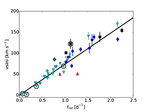
Figure 14: The correlation between the spectroscopic $v\sin i$ values and the values of the rotation rate $f_{\rm rot}$ which were derived in this study. The black line indicates the corresponding linear fit, for which the coefficients are listed in Table 3. The used symbols are the same as in Fig. 11. For all of the stars a series of prograde dipole modes was detected. If another series was detected as well, the symbol of the corresponding mode identification was used.

5 Discussion and conclusions

In this paper, we have presented methodology to derive the near-core interior rotation rate $f_{\rm rot}$ from an observed period spacing pattern and to perform mode identification for the pulsations in the series. In a first step, we considered all combinations of $l$- and $m$-values for mode identification. For each pair of $(l,m)$we consider the asymptotic spacing $\Delta\Pi_{l}$ and compute the corresponding equidistant model period spacing pattern as described by Tassoul (1980). Using the traditional approximation, the frequencies of the model pattern are subsequently shifted for an assumed rotation rate $f_{\rm rot}$ and the chosen $l$ and $m$. The optimal values of $\Delta\Pi_{l}$, $f_{\rm rot}$, $l$ and $m$ are then determined by fitting the model pattern to the observed period spacing series using least-squares optimisation and taking into account that different values of $\Delta\Pi_{l}$ are expected for different values of $l$.

In most cases this method is reasonably successful. For slow rotators it may be difficult to find the correct value for the azimuthal order $m$, though this problem is solved when we have multiple series with different $l$ and $m$ values. By fitting these series simultaneously, not only do we obtain the mode identification, but the values for $\Delta\Pi_{l}$ and $f_{\rm rot}$ are also a lot more precise than in the case where we do not detect multiplets. In the case where we are dealing with a moderate to fast rotator, the retrograde modes were found to be Rossby modes, which arise due to the interaction between the stellar rotation and toroidal modes. In this study, we have used the asymptotic approximation derived by Townsend (2003b) to compute their eigenvalues $\lambda$ of the Laplace tidal equation. A complete numerical treatment of these modes is required to exploit them quantitatively. A complete and detailed analysis of such stars with multiple gravity-mode period spacings will allow us to study possible differential rotation in $\gamma$ Dor stars, ultimately leading to proper observational constraints on rotational chemical mixing and angular momentum transport mechanisms.

From the ensemble modelling of the gravity-mode period spacings of the stars in our sample, we found that there is a large range in the stellar rotation rates. Interestingly, only three out of forty targets were found to be in the superinertial regime. These three stars, KIC 8645874, KIC 9751996 and KIC 11754232, are hybrid $\gamma$ Dor/$\delta$ Sct stars which exhibit variability in the frequency range from 5 $\rm d^{-1}$ to 8 $\rm d^{-1}$. This indicates that these stars’ low rotation rates are likely linked to their hybrid character, making them prime targets for further asteroseismological analysis. The other stars were found to be in the subinertial regime. Their pulsation frequencies in the corotating frame are typically confined in the narrow range between 0.15 and 0.75 $\rm d^{-1}$. This is in agreement with the theoretical expectation that $\gamma$ Dor pulsation frequencies in the corotating frame are on the order of the thermal timescale $\tau_{th}$ at the bottom of the convective envelope (Bouabid et al. 2013). However, this frequency range does not agree with the predicted values by Bouabid et al. (2013). With the exception of the three stars in the superinertial regime, we find that on average the observed modes have longer pulsation periods in the corotating frame than theory predicts. This is also reflected in the high spin parameter values we derived for many of the stars. The high spin parameters detected for the retrograde Rossby modes are linked to the low eigenvalues $\lambda$ of these modes as already found on theoretical grounds by Townsend (2003b).

The global results for the mode identification are consistent with existing spectroscopic studies. The majority of the modes were found to be prograde dipole modes. This is in line with the results obtained by Townsend (2003a) for heat-driven gravity modes in slowly pulsating B stars. In addition, we found single high-amplitude modes, as opposed to a series, to be present in several stars. They are consistent with retrograde Rossby modes with $m=-1$. They are likely heavily influenced by mode trapping, and as a result contain valuable information about these stars’ internal structure.

We conducted a linear regression analysis on the combined spectroscopic and photometric parameter values for the sample. The strong correlation between $v\sin i$ and $f_{\rm rot}$ independently confirmed the reliability of the obtained rotation rates. We also detected weak correlations between $R\sin i=v\sin i/f_{\rm rot}$ and $T_{\rm eff}$ and between $\log\,g$ and $f_{\rm rot}$. Indeed, as a star with a convective core evolves on the main sequence, its radius increases, and its temperature and rotation rate decrease.

Despite the limitations of the traditional approximation, the results we obtained in this work are consistent and offer the first estimates of the interior rotation frequencies for a large sample of $\gamma\,$Dor stars. The large observed spin parameter values indicate that the pulsations are constrained in a waveguide around the equator (Townsend 2003a, b). This in turn implies that the vast majority of the stars should be seen at moderate to high inclination angles, which is also what we can indirectly derive from the relation between the observed $v\sin i$ and $f_{\rm rot}$ in Fig. 14. From the grid of theoretical models in Section 2, we find radii between 1.3 $R_{\odot}$ and 3 $R_{\odot}$. For many stars in our sample, this results in inclination angle estimates on the order of or above 50 °. Two of the stars for which lower inclination angle estimates were found, KIC 4846809 and KIC 9595743, are also the stars for which we detected zonal dipole modes. This is consistent with expectations for the geometrical cancellation effects of the pulsations.

These ensemble analyses now form an ideal starting point for detailed asteroseismological modelling of individual targets in the sample. This, in turn, will allow us to place constraints on the shape and extent of the convective core overshooting and the diffusive mixing processes in the radiative near-core regions, and by extension on the evolution of the convective core itself as it was recently achieved for a hybrid $\delta\,$Sct — $\gamma\,$Dor binary (Schmid & Aerts 2016) and also for a slowly (Moravveji et al. 2015) and a moderately (Moravveji et al. 2016) rotating gravity-mode pulsator of $\sim$ 3.3 $M_{\odot}$.

Appendix A Simulated period spacing pattern

Table 4: The pulsation periods (in days; in the inertial reference frame) of the simulated data in Section 4.1, with the used 1$\sigma$ uncertainty margins.

$P_{\rm inert}$ [$d$]	$\sigma_{P}$	$P_{\rm inert}$ [$d$]	$\sigma_{P}$
0.73912	0.00004	0.91909	0.00002
0.751414	0.000008	0.92658	0.00006
0.76322	0.00005	0.93385	0.00004
0.774892	0.000007	0.94088	0.00001
0.78640	0.00003	0.94772	0.00001
0.79748	0.00006	0.95442	0.00007
0.80785	0.00001	0.96100	0.00004
0.81753	0.00005	0.96745	0.00006
0.82691	0.00004	0.97373	0.00006
0.83618	0.00004	0.97984	0.00001
0.84513	0.00006	0.98579	0.00006
0.85371	0.00003	0.99161	0.00008
0.86220	0.00006	0.99732	0.00003
0.87080	0.00003	1.00292	0.00008
0.87937	0.00004	1.00839	0.00005
0.88773	0.00008	1.01372	0.00009
0.89582	0.00003	1.01891	0.00004
0.903689	0.000007	1.02400	0.00008
0.91144	0.00001	1.02898	0.00006

Appendix B Stellar rotation rates and mode identification

Table 5: The rotation rates $f_{\rm rot}$ and the asymptotic period spacings $\Delta\Pi_{l}$ which were computed from the observed period spacing patterns, as well as the mode identification and the dominant pulsation frequency for each series. For the latter we also computed the spin parameter $s$, listed in the final column. The pulsation mode patterns which are marked with “R” are retrograde modes, which are most likely Rossby modes. The pulsation modes which are marked with “S” are single high-amplitude peaks which were present in the frequency spectra, but clearly separate from the detected period spacing patterns. Neither the retrograde pulsation modes nor the single peaks were actually used in the computations. The corresponding rotation rates and asymptotic period spacings were obtained from the prograde series observed for the same star.

KIC	$l$	$m$	$f_{\rm dom,inert}$		$f_{\rm rot}$		$\Delta\Pi_{l}$		$|s|$
			[$\rm d^{-1}$]	[$\mu$Hz]	[$\rm d^{-1}$]	[$\mu$Hz]	[s]	[d]
2710594	$1$	$1$	$1.35536^{+0.00001}_{-0.00001}$	$15.68706^{+0.00012}_{-0.00012}$	$1.02^{+0.02}_{-0.02}$	$11.8^{+0.2}_{-0.3}$	$3370^{+330}_{-310}$	$0.039^{+0.004}_{-0.004}$	$6.2^{+0.5}_{-0.5}$
	R	R	$0.79908^{+0.00002}_{-0.00002}$	$9.24856^{+0.00022}_{-0.00022}$	$1.02^{+0.02}_{-0.02}$	$11.8^{+0.2}_{-0.3}$	$3370^{+330}_{-310}$	$0.039^{+0.004}_{-0.004}$	$9.1^{+0.7}_{-0.6}$
3448365	$1$	$1$	$1.500157^{+0.000009}_{-0.000009}$	$17.36293^{+0.00010}_{-0.00010}$	$1.08^{+0.05}_{-0.07}$	$12.5^{+0.6}_{-0.8}$	$3020^{+1160}_{-970}$	$0.03^{+0.01}_{-0.01}$	$5.2^{+0.9}_{-1.2}$
	R	R	$0.88877^{+0.00001}_{-0.00001}$	$10.28675^{+0.00016}_{-0.00016}$	$1.08^{+0.05}_{-0.07}$	$12.5^{+0.6}_{-0.8}$	$3020^{+1160}_{-970}$	$0.03^{+0.01}_{-0.01}$	$11^{+4}_{-3}$
4846809	$1$	$1$	$1.81324^{+0.00001}_{-0.00001}$	$20.98662^{+0.00014}_{-0.00014}$	$1.28^{+0.01}_{-0.02}$	$14.8^{+0.2}_{-0.2}$	$2930^{+140}_{-150}$	$0.034^{+0.002}_{-0.002}$	$4.8^{+0.2}_{-0.2}$
	$1$	$0$	$1.00410^{+0.00002}_{-0.00002}$	$11.62156^{+0.00024}_{-0.00024}$	$1.28^{+0.01}_{-0.02}$	$14.8^{+0.2}_{-0.2}$	$2930^{+140}_{-150}$	$0.034^{+0.002}_{-0.002}$	$2.55^{+0.03}_{-0.03}$
5114382	$1$	$1$	$1.47927^{+0.00002}_{-0.00002}$	$17.12115^{+0.00020}_{-0.00020}$	$1.15^{+0.02}_{-0.02}$	$13.3^{+0.2}_{-0.2}$	$3070^{+300}_{-290}$	$0.036^{+0.003}_{-0.003}$	$7.0^{+0.5}_{-0.6}$
	R	R	$0.95265^{+0.00002}_{-0.00002}$	$11.02607^{+0.00018}_{-0.00018}$	$1.15^{+0.02}_{-0.02}$	$13.3^{+0.2}_{-0.2}$	$3070^{+300}_{-290}$	$0.036^{+0.003}_{-0.003}$	$11.6^{+1.0}_{-0.9}$
5522154	$1$	$1$	$3.009858^{+0.000008}_{-0.000008}$	$34.83632^{+0.00009}_{-0.00009}$	$2.154^{+0.004}_{-0.004}$	$24.93^{+0.05}_{-0.05}$	$3350^{+40}_{-30}$	$0.0388^{+0.0004}_{-0.0004}$	$5.03^{+0.03}_{-0.03}$
5708550	$1$	$1$	$1.11550^{+0.00001}_{-0.00001}$	$12.91091^{+0.00014}_{-0.00014}$	$0.82^{+0.01}_{-0.02}$	$9.4^{+0.2}_{-0.2}$	$3330^{+240}_{-220}$	$0.039^{+0.003}_{-0.003}$	$5.5^{+0.4}_{-0.4}$
5788623	$1$	$1$	$0.77895^{+0.00001}_{-0.00001}$	$9.01558^{+0.00014}_{-0.00014}$	$0.40^{+0.04}_{-0.05}$	$4.6^{+0.5}_{-0.5}$	$2800^{+480}_{-440}$	$0.032^{+0.006}_{-0.005}$	$2.1^{+0.4}_{-0.5}$
6468146	$1$	$1$	$1.545700^{+0.000005}_{-0.000005}$	$17.89004^{+0.00005}_{-0.00005}$	$0.97^{+0.01}_{-0.01}$	$11.3^{+0.1}_{-0.2}$	$3000^{+110}_{-110}$	$0.035^{+0.001}_{-0.001}$	$3.4^{+0.1}_{-0.1}$
6468987	$1$	$1$	$1.998989^{+0.000004}_{-0.000004}$	$23.13644^{+0.00005}_{-0.00005}$	$1.598^{+0.009}_{-0.008}$	$18.49^{+0.10}_{-0.09}$	$3730^{+120}_{-100}$	$0.043^{+0.001}_{-0.001}$	$8.0^{+0.2}_{-0.2}$
	R	R	$1.387598^{+0.000009}_{-0.000009}$	$16.06016^{+0.00011}_{-0.00011}$	$1.598^{+0.009}_{-0.008}$	$18.49^{+0.10}_{-0.09}$	$3730^{+120}_{-100}$	$0.043^{+0.001}_{-0.001}$	$15.2^{+0.5}_{-0.6}$
6678174	$1$	$1$	$1.12777^{+0.00002}_{-0.00002}$	$13.05290^{+0.00020}_{-0.00020}$	$0.55^{+0.05}_{-0.06}$	$6.4^{+0.6}_{-0.7}$	$3370^{+710}_{-620}$	$0.039^{+0.008}_{-0.007}$	$1.9^{+0.4}_{-0.4}$
6935014	$1$	$1$	$1.20670^{+0.00001}_{-0.00001}$	$13.96648^{+0.00014}_{-0.00014}$	$0.79^{+0.02}_{-0.02}$	$9.1^{+0.2}_{-0.3}$	$3180^{+310}_{-300}$	$0.037^{+0.004}_{-0.003}$	$3.8^{+0.3}_{-0.3}$
6953103	$1$	$1$	$1.287597^{+0.000008}_{-0.000008}$	$14.90274^{+0.00009}_{-0.00009}$	$0.74^{+0.03}_{-0.04}$	$8.5^{+0.4}_{-0.4}$	$3560^{+490}_{-440}$	$0.041^{+0.006}_{-0.005}$	$2.7^{+0.3}_{-0.3}$
7023122	$1$	$1$	$1.876108^{+0.000003}_{-0.000003}$	$21.71421^{+0.00003}_{-0.00003}$	$0.977^{+0.005}_{-0.005}$	$11.30^{+0.06}_{-0.06}$	$3380^{+40}_{-30}$	$0.0391^{+0.0004}_{-0.0004}$	$2.17^{+0.03}_{-0.03}$
7365537	$1$	$1$	$2.925633^{+0.000004}_{-0.000004}$	$33.86150^{+0.00004}_{-0.00004}$	$2.253^{+0.003}_{-0.003}$	$26.07^{+0.03}_{-0.03}$	$3340^{+30}_{-30}$	$0.0387^{+0.0003}_{-0.0003}$	$6.70^{+0.04}_{-0.04}$
	S	S	$1.981016^{+0.000006}_{-0.000006}$	$22.92843^{+0.00006}_{-0.00006}$	$2.253^{+0.003}_{-0.003}$	$26.07^{+0.03}_{-0.03}$	$3340^{+30}_{-30}$	$0.0387^{+0.0003}_{-0.0003}$	$16.6^{+0.2}_{-0.2}$
7380501	$1$	$1$	$0.96329^{+0.00001}_{-0.00001}$	$11.14922^{+0.00012}_{-0.00012}$	$0.64^{+0.01}_{-0.01}$	$7.4^{+0.2}_{-0.2}$	$2860^{+180}_{-170}$	$0.033^{+0.002}_{-0.002}$	$3.9^{+0.2}_{-0.3}$
7434470	$1$	$1$	$2.542409^{+0.000006}_{-0.000006}$	$29.42603^{+0.00007}_{-0.00007}$	$1.769^{+0.005}_{-0.005}$	$20.47^{+0.06}_{-0.06}$	$3020^{+50}_{-50}$	$0.0349^{+0.0006}_{-0.0005}$	$4.57^{+0.04}_{-0.04}$
	S	S	$1.698729^{+0.000001}_{-0.000001}$	$19.66122^{+0.00002}_{-0.00002}$	$1.769^{+0.005}_{-0.005}$	$20.47^{+0.06}_{-0.06}$	$3020^{+50}_{-50}$	$0.0349^{+0.0006}_{-0.0005}$	$50^{+3}_{-4}$
7583663	$1$	$1$	$1.47213^{+0.00001}_{-0.00001}$	$17.03853^{+0.00017}_{-0.00017}$	$1.17^{+0.02}_{-0.03}$	$13.6^{+0.3}_{-0.3}$	$3120^{+390}_{-360}$	$0.036^{+0.005}_{-0.004}$	$7.8^{+0.8}_{-0.9}$
	R	R	$1.044741^{+0.000008}_{-0.000008}$	$12.09190^{+0.00009}_{-0.00009}$	$1.17^{+0.02}_{-0.03}$	$13.6^{+0.3}_{-0.3}$	$3120^{+390}_{-360}$	$0.036^{+0.005}_{-0.004}$	$19^{+3}_{-3}$
7746984	$1$	$1$	$2.00305^{+0.00002}_{-0.00002}$	$23.18341^{+0.00019}_{-0.00019}$	$1.49^{+0.02}_{-0.02}$	$17.2^{+0.2}_{-0.2}$	$3130^{+250}_{-230}$	$0.036^{+0.003}_{-0.003}$	$5.8^{+0.3}_{-0.3}$
	S	S	$1.35180^{+0.00001}_{-0.00001}$	$15.64582^{+0.00014}_{-0.00014}$	$1.49^{+0.02}_{-0.02}$	$17.2^{+0.2}_{-0.2}$	$3130^{+250}_{-230}$	$0.036^{+0.003}_{-0.003}$	$22^{+3}_{-2}$
7939065	$1$	$1$	$1.728171^{+0.000007}_{-0.000007}$	$20.00198^{+0.00008}_{-0.00008}$	$1.111^{+0.006}_{-0.006}$	$12.86^{+0.07}_{-0.07}$	$3000^{+40}_{-40}$	$0.0347^{+0.0005}_{-0.0005}$	$3.60^{+0.05}_{-0.05}$
8364249	$1$	$1$	$1.869376^{+0.000005}_{-0.000005}$	$21.63629^{+0.00005}_{-0.00005}$	$1.519^{+0.007}_{-0.008}$	$17.58^{+0.08}_{-0.09}$	$3090^{+110}_{-110}$	$0.036^{+0.001}_{-0.001}$	$8.7^{+0.2}_{-0.2}$
8375138	$1$	$1$	$2.077771^{+0.000007}_{-0.000007}$	$24.04828^{+0.00008}_{-0.00008}$	$1.64^{+0.01}_{-0.01}$	$19.0^{+0.1}_{-0.1}$	$2930^{+150}_{-150}$	$0.034^{+0.002}_{-0.002}$	$7.5^{+0.3}_{-0.3}$
	R	R	$1.407115^{+0.000010}_{-0.000010}$	$16.28606^{+0.00011}_{-0.00011}$	$1.64^{+0.01}_{-0.01}$	$19.0^{+0.1}_{-0.1}$	$2930^{+150}_{-150}$	$0.034^{+0.002}_{-0.002}$	$14.0^{+0.7}_{-0.6}$
8645874	$1$	$1$	$1.847014^{+0.000004}_{-0.000004}$	$21.37747^{+0.00005}_{-0.00005}$	$0.375^{+0.002}_{-0.002}$	$4.34^{+0.02}_{-0.02}$	$3200^{+10}_{-10}$	$0.0371^{+0.0001}_{-0.0001}$	$0.510^{+0.003}_{-0.003}$
8836473	$1$	$1$	$1.88341^{+0.00001}_{-0.00001}$	$21.79871^{+0.00012}_{-0.00012}$	$1.13^{+0.01}_{-0.01}$	$13.0^{+0.2}_{-0.2}$	$2900^{+100}_{-100}$	$0.034^{+0.001}_{-0.001}$	$2.98^{+0.09}_{-0.09}$
	S	S	$0.52525^{+0.00001}_{-0.00001}$	$6.07932^{+0.00015}_{-0.00015}$	$1.13^{+0.01}_{-0.01}$	$13.0^{+0.2}_{-0.2}$	$2900^{+100}_{-100}$	$0.034^{+0.001}_{-0.001}$	$3.75^{+0.04}_{-0.04}$
9210943	$1$	$1$	$2.190853^{+0.000004}_{-0.000004}$	$25.35710^{+0.00005}_{-0.00005}$	$1.728^{+0.007}_{-0.010}$	$19.99^{+0.09}_{-0.11}$	$3340^{+80}_{-100}$	$0.0386^{+0.0010}_{-0.0012}$	$7.5^{+0.2}_{-0.2}$
	R	R	$1.443566^{+0.000009}_{-0.000009}$	$16.70794^{+0.00011}_{-0.00011}$	$1.728^{+0.007}_{-0.010}$	$19.99^{+0.09}_{-0.11}$	$3340^{+80}_{-100}$	$0.0386^{+0.0010}_{-0.0012}$	$12.2^{+0.3}_{-0.3}$
9480469	$1$	$1$	$1.994822^{+0.000010}_{-0.000010}$	$23.08821^{+0.00011}_{-0.00011}$	$1.54^{+0.03}_{-0.03}$	$17.8^{+0.3}_{-0.3}$	$2990^{+410}_{-360}$	$0.035^{+0.005}_{-0.004}$	$6.8^{+0.5}_{-0.6}$
	R	R	$1.32598^{+0.00001}_{-0.00001}$	$15.34704^{+0.00012}_{-0.00012}$	$1.54^{+0.03}_{-0.03}$	$17.8^{+0.3}_{-0.3}$	$2990^{+410}_{-360}$	$0.035^{+0.005}_{-0.004}$	$14^{+2}_{-2}$
9595743	$1$	$1$	$1.43459^{+0.00002}_{-0.00002}$	$16.6040^{+0.0002}_{-0.0002}$	$0.89^{+0.01}_{-0.01}$	$10.3^{+0.1}_{-0.1}$	$3050^{+110}_{-110}$	$0.035^{+0.001}_{-0.001}$	$3.3^{+0.1}_{-0.1}$
	$1$	$0$	$1.16055^{+0.00002}_{-0.00002}$	$13.43228^{+0.00019}_{-0.00019}$	$0.89^{+0.01}_{-0.01}$	$10.3^{+0.1}_{-0.1}$	$3050^{+110}_{-110}$	$0.035^{+0.001}_{-0.001}$	$1.54^{+0.02}_{-0.02}$
9751996	$1$	$1$	$1.35387^{+0.00002}_{-0.00002}$	$15.6698^{+0.0002}_{-0.0002}$	$0.0696^{+0.0008}_{-0.0008}$	$0.805^{+0.010}_{-0.010}$	$3086^{+6}_{-6}$	$0.03572^{+0.00007}_{-0.00007}$	$0.11^{+0.03}_{-0.03}$
	$1$	$0$	$1.02805^{+0.00002}_{-0.00002}$	$11.8987^{+0.0002}_{-0.0002}$	$0.0696^{+0.0008}_{-0.0008}$	$0.805^{+0.010}_{-0.010}$	$3086^{+6}_{-6}$	$0.03572^{+0.00007}_{-0.00007}$	$0.14^{+0.03}_{-0.03}$
	$1$	$-1$	$1.28331^{+0.00002}_{-0.00002}$	$14.8531^{+0.0002}_{-0.0002}$	$0.0696^{+0.0008}_{-0.0008}$	$0.805^{+0.010}_{-0.010}$	$3086^{+6}_{-6}$	$0.03572^{+0.00007}_{-0.00007}$	$0.11^{+0.03}_{-0.03}$
10256787	$1$	$1$	$1.077489^{+0.000008}_{-0.000008}$	$12.47094^{+0.00009}_{-0.00009}$	$0.59^{+0.04}_{-0.04}$	$6.9^{+0.4}_{-0.5}$	$2730^{+560}_{-490}$	$0.032^{+0.006}_{-0.006}$	$2.5^{+0.3}_{-0.4}$
10467146	$1$	$1$	$0.954976^{+0.000009}_{-0.000009}$	$11.05297^{+0.00011}_{-0.00011}$	$0.62^{+0.03}_{-0.04}$	$7.1^{+0.4}_{-0.5}$	$2940^{+600}_{-540}$	$0.034^{+0.007}_{-0.006}$	$3.6^{+0.6}_{-0.7}$
11080103	$1$	$1$	$1.241393^{+0.000005}_{-0.000005}$	$14.36797^{+0.00006}_{-0.00006}$	$0.62^{+0.05}_{-0.06}$	$7.2^{+0.6}_{-0.7}$	$3360^{+880}_{-730}$	$0.039^{+0.010}_{-0.008}$	$2.0^{+0.3}_{-0.4}$
11099031	$1$	$1$	$1.61508^{+0.00001}_{-0.00001}$	$18.69302^{+0.00014}_{-0.00014}$	$1.025^{+0.009}_{-0.009}$	$11.87^{+0.10}_{-0.10}$	$3560^{+100}_{-110}$	$0.041^{+0.001}_{-0.001}$	$3.48^{+0.08}_{-0.08}$
	S	S	$0.916646^{+0.000009}_{-0.000009}$	$10.60933^{+0.00010}_{-0.00010}$	$1.025^{+0.009}_{-0.009}$	$11.87^{+0.10}_{-0.10}$	$3560^{+100}_{-110}$	$0.041^{+0.001}_{-0.001}$	$19^{+1}_{-1}$
11294808	$1$	$1$	$1.16617^{+0.00001}_{-0.00001}$	$13.49738^{+0.00014}_{-0.00014}$	$0.77^{+0.02}_{-0.02}$	$9.0^{+0.2}_{-0.3}$	$2770^{+350}_{-320}$	$0.032^{+0.004}_{-0.004}$	$4.0^{+0.3}_{-0.4}$
	$2$	$2$	$2.2247^{+0.0007}_{-0.0007}$	$25.749^{+0.008}_{-0.008}$	$0.77^{+0.02}_{-0.02}$	$9.0^{+0.2}_{-0.3}$	$1600^{+200}_{--190}$	$0.019^{+0.002}_{-0.002}$	$2.3^{+0.2}_{-0.2}$
11456474	$1$	$1$	$1.471468^{+0.000006}_{-0.000006}$	$17.03088^{+0.00007}_{-0.00007}$	$1.05^{+0.02}_{-0.02}$	$12.2^{+0.2}_{-0.2}$	$2810^{+250}_{-240}$	$0.033^{+0.003}_{-0.003}$	$5.0^{+0.3}_{-0.3}$
11721304	$1$	$1$	$0.92287^{+0.00002}_{-0.00002}$	$10.68141^{+0.00020}_{-0.00020}$	$0.46^{+0.03}_{-0.03}$	$5.3^{+0.4}_{-0.4}$	$3080^{+430}_{-400}$	$0.036^{+0.005}_{-0.005}$	$2.0^{+0.3}_{-0.3}$
11754232	$1$	$1$	$1.10338^{+0.00001}_{-0.00001}$	$12.77065^{+0.00017}_{-0.00017}$	$0.159^{+0.007}_{-0.007}$	$1.84^{+0.08}_{-0.09}$	$3130^{+20}_{-20}$	$0.0362^{+0.0002}_{-0.0003}$	$0.34^{+0.02}_{-0.02}$
11826272	$1$	$1$	$0.83370^{+0.00001}_{-0.00001}$	$9.64927^{+0.00013}_{-0.00013}$	$0.36^{+0.02}_{-0.03}$	$4.1^{+0.3}_{-0.3}$	$2950^{+290}_{-280}$	$0.034^{+0.003}_{-0.003}$	$1.5^{+0.2}_{-0.2}$
11907454	$1$	$1$	$1.77890^{+0.00001}_{-0.00001}$	$20.58915^{+0.00016}_{-0.00016}$	$1.35^{+0.02}_{-0.02}$	$15.6^{+0.2}_{-0.3}$	$3050^{+290}_{-280}$	$0.035^{+0.003}_{-0.003}$	$6.2^{+0.4}_{-0.4}$
	R	R	$1.187153^{+0.000008}_{-0.000008}$	$13.74020^{+0.00009}_{-0.00009}$	$1.35^{+0.02}_{-0.02}$	$15.6^{+0.2}_{-0.3}$	$3050^{+290}_{-280}$	$0.035^{+0.003}_{-0.003}$	$17^{+2}_{-2}$
11917550	$1$	$1$	$1.287680^{+0.000008}_{-0.000008}$	$14.90371^{+0.00010}_{-0.00010}$	$0.90^{+0.02}_{-0.02}$	$10.4^{+0.2}_{-0.2}$	$2900^{+220}_{-210}$	$0.034^{+0.003}_{-0.002}$	$4.6^{+0.3}_{-0.3}$
11920505	$1$	$1$	$1.198844^{+0.000009}_{-0.000009}$	$13.87550^{+0.00010}_{-0.00010}$	$0.75^{+0.02}_{-0.02}$	$8.7^{+0.2}_{-0.3}$	$2980^{+260}_{-250}$	$0.035^{+0.003}_{-0.003}$	$3.3^{+0.2}_{-0.3}$
12066947	$1$	$1$	$2.72379^{+0.00001}_{-0.00001}$	$31.52539^{+0.00015}_{-0.00015}$	$2.160^{+0.008}_{-0.008}$	$25.00^{+0.09}_{-0.10}$	$2950^{+70}_{-70}$	$0.0342^{+0.0008}_{-0.0008}$	$7.7^{+0.1}_{-0.1}$
	R	R	$1.88748^{+0.00002}_{-0.00002}$	$21.8459^{+0.0002}_{-0.0002}$	$2.160^{+0.008}_{-0.008}$	$25.00^{+0.09}_{-0.10}$	$2950^{+70}_{-70}$	$0.0342^{+0.0008}_{-0.0008}$	$15.8^{+0.4}_{-0.4}$

Appendix C Sample analysis

References

• Aerts et al. (2010) Aerts, C., Christensen-Dalsgaard, J., & Kurtz, D. W. 2010, Asteroseismology, Astronomy and Astrophsyics Library, Springer Berlin Heidelberg
• Asplund et al. (2009) Asplund, M., Grevesse, N., Sauval, A. J., & Scott, P. 2009, ARA&A, 47, 481
• Auvergne et al. (2009) Auvergne, M., Bodin, P., Boisnard, L., et al. 2009, A&A, 506, 411
• Ballot et al. (2012) Ballot, J., Lignières, F., Prat, V., Reese, D. R., & Rieutord, M. 2012, in Astronomical Society of the Pacific Conference Series, Vol. 462, Progress in Solar/Stellar Physics with Helio- and Asteroseismology, ed. H. Shibahashi, M. Takata, & A. E. Lynas-Gray, 389
• Bedding et al. (2015) Bedding, T. R., Murphy, S. J., Colman, I. L., & Kurtz, D. W. 2015, in European Physical Journal Web of Conferences, Vol. 101, European Physical Journal Web of Conferences, 01005
• Bouabid et al. (2013) Bouabid, M.-P., Dupret, M.-A., Salmon, S., et al. 2013, MNRAS, 429, 2500
• Chapellier et al. (2012) Chapellier, E., Mathias, P., Weiss, W. W., Le Contel, D., & Debosscher, J. 2012, A&A, 540, A117
• Dupret et al. (2005) Dupret, M.-A., Grigahcène, A., Garrido, R., Gabriel, M., & Scuflaire, R. 2005, A&A, 435, 927
• Dziembowski & Pamyatnykh (1991) Dziembowski, W. A. & Pamyatnykh, A. A. 1991, A&A, 248, L11
• Eckart (1960) Eckart, G. 1960, Hydrodynamics of oceans and atmospheres, Pergamon Press, Oxford
• Guzik et al. (2000) Guzik, J. A., Kaye, A. B., Bradley, P. A., Cox, A. N., & Neuforge, C. 2000, ApJ, 542, L57
• Kaye et al. (1999) Kaye, A. B., Handler, G., Krisciunas, K., Poretti, E., & Zerbi, F. M. 1999, PASP, 111, 840
• Keen et al. (2015) Keen, M. A., Bedding, T. R., Murphy, S. J., et al. 2015, MNRAS, 454, 1792
• Koch et al. (2010) Koch, D. G., Borucki, W. J., Basri, G., et al. 2010, ApJ, 713, L79
• Kurtz et al. (2014) Kurtz, D. W., Saio, H., Takata, M., et al. 2014, MNRAS, 444, 102
• Lee & Saio (1987) Lee, U. & Saio, H. 1987, MNRAS, 224, 513
• Lee & Saio (1997) Lee, U. & Saio, H. 1997, ApJ, 491, 839
• Maeder & Meynet (2000) Maeder, A. & Meynet, G. 2000, A&A, 361, 159
• Miglio et al. (2008) Miglio, A., Montalbán, J., Noels, A., & Eggenberger, P. 2008, MNRAS, 386, 1487
• Moravveji et al. (2015) Moravveji, E., Aerts, C., Pápics, P. I., Triana, S. A., & Vandoren, B. 2015, A&A, 580, A27
• Moravveji et al. (2016) Moravveji, E., Townsend, R. H. D., Aerts, C., & Mathis, S. 2016, ApJ, 823, 130
• Murphy et al. (2016) Murphy, S. J., Fossati, L., Bedding, T. R., et al. 2016, MNRAS, 459, 1201
• Papaloizou & Pringle (1978) Papaloizou, J. & Pringle, J. E. 1978, MNRAS, 182, 423
• Paxton et al. (2011) Paxton, B., Bildsten, L., Dotter, A., et al. 2011, ApJS, 192, 3
• Paxton et al. (2013) Paxton, B., Cantiello, M., Arras, P., et al. 2013, ApJS, 208, 4
• Paxton et al. (2015) Paxton, B., Marchant, P., Schwab, J., et al. 2015, ApJS, 220, 15
• Rogers & Nayfonov (2002) Rogers, F. J. & Nayfonov, A. 2002, ApJ, 576, 1064
• Rogers (2015) Rogers, T. M. 2015, ApJ, 815, L30
• Saio et al. (2015) Saio, H., Kurtz, D. W., Takata, M., et al. 2015, MNRAS, 447, 3264
• Schmid & Aerts (2016) Schmid, V. S. & Aerts, C. 2016, A&A, in press (arXiv:1605.07958)
• Silva Aguirre et al. (2011) Silva Aguirre, V., Ballot, J., Serenelli, A. M., & Weiss, A. 2011, A&A, 529, A63
• Tassoul (1980) Tassoul, M. 1980, ApJS, 43, 469
• Townsend (2003a) Townsend, R. H. D. 2003a, MNRAS, 343, 125
• Townsend (2003b) Townsend, R. H. D. 2003b, MNRAS, 340, 1020
• Townsend (2005) Townsend, R. H. D. 2005, MNRAS, 360, 465
• Townsend & Teitler (2013) Townsend, R. H. D. & Teitler, S. A. 2013, MNRAS, 435, 3406
• Triana et al. (2015) Triana, S. A., Moravveji, E., Pápics, P. I., et al. 2015, ApJ, 810, 16
• Van Reeth et al. (2015) Van Reeth, T., Tkachenko, A., Aerts, C., et al. 2015, ApJS, 218, 27
• Walker et al. (2003) Walker, G., Matthews, J., Kuschnig, R., et al. 2003, Publications of the Astronomical Society of the Pacific, 115, 1023
• Xiong et al. (2016) Xiong, D. R., Deng, L., Zhang, C., & Wang, K. 2016, MNRAS, 457, 3163