A New Method to Optimize Finite Dimensions Thermodynamic Models: application to an Irreversible Stirling Engine

Abstract

Different economical configurations, due for instance to the relative cost of the fuel it consumes, can push a heat engine into operating whether at maximum efficiency or at maximum power produced. Any relevant design of such system hence needs to be based, at least partly, on the knowledge of its specific ”power vs. efficiency” characteristic curve. However, even when a simple model is used to describe the engine, obtained for example thanks to Finite Dimensions Thermodynamics, such characteristic curve is often difficult to obtain and takes an explicit form only for the simplest of these models. When more realistic models are considered, including complex internal subsystems or processes, an explicit expression for this curve is practically impossible to obtain. In this paper, we propose to use the called Graham’s scan algorithm in order to directly obtain the power vs. efficiency curve of a realistic Stirling engine model, which includes heat leakage, regenerator effectiveness, as well as internal and external irreversibilities. Coupled with an adapted optimization routine, this approach allows to design and optimize the same way simple or complex heat engine models. Such method can then be useful during the practical design task of any thermal power converter, almost regardless to its own internal complexity.

PACS numbers : 05.70.Ln, 84.60.Bk, 88.05.Bc, 88.05.De

Keywords : Finite Dimension Thermodynamics; Stirling Engines; Optimization; Convex hull.

1 Introduction

Air Engines, i.e. Stirling and Ericsson ones, can help to solve various energy problems. They can be supplied by different kinds of heat sources (combustion, solar or nuclear energy) and they are usually quiet, at least when compared to Internal Combustion Engines. Benefiting from these good points, such engines can thus be included for instance in domestic cogeneration, i.e. Combined Heating and Power systems [1, 2] or in trigeneration, i.e. Combined Cooling, Heating and Power systems [3]. Stirling engines can also be used for example in solar-power plants [4], in solar-pumping systems [5] or in combined cycle with other machines [6], as e.g. high temperature fuel cells [7, 8].

Air engines operate over closed and regenerative thermodynamic cycles, with typically a permanent gas, as e.g. helium or air as working fluid. It means that, among other complex components, very specific heat exchangers have to be designed in order to exchange the required heat quantities between the working gas and the hot and cold sources of the engine; but also from this gas to itself at a different moment of the cycle, thanks to a regenerator [9].

Before the use of a complete but complex engine model — such as those presented for example in [10, 11] — which requires a lot of information sometimes not already available, a simpler model, based for example on Finite Dimensions Thermodynamics [12, 13] can help to design such systems. This kind of model can thus be used for sort of preliminary designs, for example to obtain a first draft of the relation between the power produced by the engine and its corresponding efficiency, so the usually called ”power vs. efficiency” or $(\eta,\dot{W})$ characteristic curve.

Such curve is really important, because once it is known, the final selected trade-off between a maximum efficiency and a maximum power produced by the whole engine must be obtained as the result of an economical calculation. Broadly explained, the higher the cost of the fuel consumed, the higher the required efficiency for the whole system, although the higher its size and so its investment cost. Indeed, for a heat engine for example, increasing its efficiency means decreasing its internal irreversibilities by decreasing, among other things, the temperature differences within its heat exchangers, and so the sizes of the latter. At the contrary, the lower the cost of the fuel, the higher the power produced in order to decrease the investment cost as far as possible, as already explained by Novikov [14] in 1958 for nuclear plants. The knowledge, for a given engine, of its $(\eta,\dot{W})$ curve, is thus needed to complete successfully such optimization step [15].

Unfortunately, an explicit algebraic expression of such curve, of the form $\dot{W}=f(\eta)$ for example, can be obtained and drawn only for the simplest models of engines. If the complexity of the latter increases, for example because including further subsystems or processes, as regenerator or heat leaks for example, the aforementioned curve can only be obtained in an implicit way, i.e. through the use of the complete model. $\dot{W}$ and $\eta$ are then two different functions of several parameters related to the engine’s design and to its operating conditions. Anyhow, without any dedicated method, this curve is nothing bu easy to obtain.

In this paper, we present a new approach, based on the called Graham’s algorithm, that allows to directly obtained the required characteristic curve with a minimal number of calls for the engine’s model. This approach will be applied to a model of Stirling engine, including different complex subsystems and phenomena.

2 Finite dimension thermodynamics of Stirling engines

Although the search for engine models dealing with maximum rates of useful energy is not really new [16, 17], such idea have been actually widely spread only after the publication of the seminal paper from Curzon and Ahlborn [18] in 1975. Since then, the method commonly called Finite Time Thermodynamics or Finite Dimensions Thermodynamics, have been applied to the optimization of numerous different energy systems [12, 13], including obviously the Stirling engine.

Radcenco et al. [19] studied the basic Stirling cycle composed by definition of four strokes : one isochoric compression, one isochoric expansion and two isothermal heat exchanges. Irreversibilities were supposed to occur during the heat exchange processes only, and were due to the transfer of a heat rate through a difference between two constant temperatures, the ones of the hot and cold thermal reservoirs and the one of the working gas. Blank et al. [20] added a regenerator to a similar model of Stirling engine, the former being considered as a usual countercurrent heat exchanger of limited effectiveness. In another paper, the same authors also introduced possible radiative heat exchange processes with the working gas in considering the same model propelled by solar energy [21]. Popescu et al. [22] generalized such model in incorporating heat leaks phenomena and an non adiabatic regenerator of limited effectiveness. Ladas and Ibrahim [23] took into account the motion of the working gas within the Stirling engine and then related the performances of the whole engine to its rotational speed. Senft [24], after obtaining a general relation for the maximum mechanical efficiency of such heat engine cycle, considering the effect of friction, applied this relation to the specific case of the Stirling engine. He considered limited values for the heat rates exchanged by the working gas and a heat leak between the hot and cold part of the engine [25]. Blank [26] generalized the same approach to a wide family of Stirling-like engine cycles. Over the years, more sophisticated Stirling engine models have been developed using Finite Dimension Thermodynamics, including the effects of pressure drop due to fluid friction inside the engine [27], inefficiencies of compression and expansion strokes [28], presence of dead volumes [29] or even actual geometries of engines [30]. It is worth noting that in all these studies, the power vs. efficiency curve was expressed as an explicit relation $\dot{W}=f(\eta)$ of a variable complexity.

3 Theoretical model

3.1 Heat transfer law

The form of the used heat transfer law influences the results obtained in the modeling of any thermodynamic system. The simplest expression for the heat transfer law is the linear one, that can be used to describe conductive or convective heat transfer processes:

$$\dot{Q}=h\cdot A\cdot\Delta T=K\cdot\Delta T$$ (1)

Where $h$ is the heat transfer coefficient, $A$ a characteristic area, $K=h\cdot A$ a thermal conductance and $\Delta T$ a temperature difference.

The linear law (1) is in good agreement with reality for laminar and turbulent convection and have been widely applied to study endoreversible and irreversible models of machines. However, for systems operating at high temperatures, radiation is the major heat transfer process. The latter is described by the Stefan-Boltzmann law, expressed for two bodies at respective temperatures $T_{1}$ and $T_{2}$, as:

$$\dot{Q}=F\cdot A\cdot\sigma\cdot\left(T_{1}^{4}-T_{2}^{4}\right)$$ (2)

With $F$ the form factor including emittance of the two bodies and view factors, and the Stefan-Boltzmann constant $\sigma=5.67\cdot 10^{-8}\,{\rm W\cdot m}^{-2}\cdot{\rm K}^{-4}$ [31]. Many thermodynamic models, including radiation, have been utilized for internal and external combustion engines, gas turbine cycles and power plants. When a system houses convective as well as radiative heat exchange processes, the Dulong-Petit law may also be useful :

$$\dot{Q}=k\cdot A\cdot\Delta T^{n}$$ (3)

With $k$ and $n$ two specific coefficients which depend on the nature of the heat transfer $n=5/4$ or $n=4/3$ for a natural laminar, or turbulent convection, on a plate respectively [32]. The Dulong-Petit law (3) have been applied to describe heat transfer in models of heat engines and refrigerators [33].

3.2 Thermodynamic cycle

The $(V,p)$ and $(S,T)$ diagrams of a Stirling-like externally and internally irreversible heat engine are shown in Figures 1 and 2, respectively.

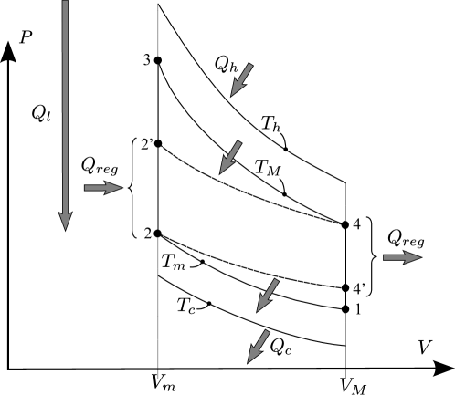
Figure 1: Representations of the Stirling cycle under study in the $(V,p)$ diagram.

The cycle operates between a heat source of constant temperature $T_{h}$ and a cold sink of constant temperature $T_{c}$. This cycle consists of two isothermal processes ($1-2$ and $3-4$) and two isochoric processes ($2-3$ and $4-1$). During the heat rejection process ($1-2$), heat flows from the working gas to a heat sink across the finite temperature difference $T_{m}-T_{c}$ and during the heat addition process ($3-4$), heat is transferred from the high temperature source across the finite difference temperature $T_{h}-T_{M}$. These two processes are thus irreversible.

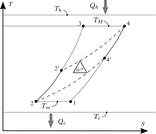
Figure 2: Representations of the Stirling cycle under study in the $(S,T)$ one. $T_{h}$ and $T_{c}$ are respectively the temperatures of the hot and cold heat sources of the engine, while $T_{M}$ and $T_{m}$ the maximum and minimum ones reached by the working gas, respectively. Thanks to a regenerator, a part $Q_{44^{\prime}}$ if the heat $Q_{41}$ rejected by the gas during its cooling process ($4-1$) is salvaged by the same fluid in order to heat up itself from $T_{2}$ to $T_{2^{\prime}}$. The remaining heat quantity $Q_{2^{\prime}3}$ required to reach the high temperature $T_{3}=T_{M}$ is supplied by the heat source at temperature $T_{h}$.

In the present study, the Stirling engine is subjected to significant losses due to heat leaks, directly from the hot source to the cold sink.

Figure 3: Schematic diagram of the system studied. The hot heat source at temperature $T_{h}$ supplies the heat rate $\dot{Q}_{h}$ to the Stirling engine through a hot heat exchanger which raise the working gas temperature at a maximum value $T_{M}$. The engine also rejects a lower heat rate $\dot{Q}_{c}$ to the cold sink at temperature $T_{c}$ through a cold heat exchanger which makes the gas temperature decrease to $T_{m}$. $\dot{Q}_{l}$ is the heat rate which leaks directly from the hot to the cold heat reservoir.

The schematic diagram in Figure 3 presents the only sizable irreversibilities taken to be heat leak between hot source and cold sink and finite rate transfer from them to the engine. All of these heat transfer processes utilize a linear model, similar as (1) because of its simplicity and because this model is as general as possible regarding to the usual practical temperature ranges of such engines.

3.3 Internal irreversibilities

Let us consider now the internal irreversibilities occurring inside the engine itself. They are due to :

• Imperfect heat exchange inside the regenerator with the working gas.

• Heat leak by conduction heat transfer between the hot and cold reservoirs.

• Heat resistances between the working gas and the heat reservoirs.

• Flow frictions between the fluid and the inner walls of the engine.

3.3.1 Regenerator with effectiveness

The regenerator

A regenerator operates as a thermal storage element, alternately absorbing and releasing heat with the working gas [9, 34, 35, 36]. In an ideal, i.e. perfectly regenerated cycle, all of the heat rejected by the working gas in order to heat up the regenerator during the constant volume phase ($4-1$) allows to later heat up the same fluid from its low to its high temperature during the cooling process of the regenerator ($2-3$), see Figure 2. The regenerator is usually designed of a porous media in order to provide the largest contact surface with the working gas. The long-awaited characteristics of such regenerative matrix are: its high heat capacity; its large contact area; its small porous matrix which minimizes the flow losses and, in minimizing dead spaces, improves the ratio of maximum to minimum pressure. In the rest, the heat quantities exchanged with the working gas are supposed to be so by a realistic non adiabatic regenerator, of effectiveness $\alpha$ [37].

The regenerator effectiveness

In general, the effectiveness defines how well a real heat exchanger is performing regarding to an ideal one operating across the same temperature difference [38]. In our case, the regenerator effectiveness $\alpha$ is thus defined as the ratio of the heat $Q_{44^{\prime}}$ rejected (or absorbed $Q_{22^{\prime}}$) by the working gas to the maximum heat $Q_{41}$ rejected (or absorbed $Q_{23}$) during the isothermal process ($4-1$) (or ($2-3$)), as presented in Figures 1 and 2.

Effectiveness $\alpha$ will be henceforth considered to be less than one but with a constant value during the heating and cooling periods, contrary to proposals of different authors [20, 39, 40]. In reality, the gas flow rate is indeed not constant and then the heat transfer coefficient between the solid matrix and the gas varies during each process of the cycle. In such situation, the efficiency cannot be constant during the cycle. Such imperfect regeneration have been modeled for example by Wu et al. [41] and the regenerator effectiveness defined by the ratio of effective and maximal energy stored or released during regenerative process [42, 43, 44].

Mathematical model of the regenerator

For the heating period of the regenerator, the effectiveness is thus:

$$\alpha=\frac{Q_{44^{\prime}}}{Q_{41}}=\frac{m\cdot c_{v}\cdot(T_{4^{\prime}}-T_{M})}{m\cdot c_{v}\cdot(T_{m}-T_{M})}\leq 1$$ (4)

Then, the working gas at the outlet of the heating period of the regenerator is:

$$T_{4^{\prime}}=T_{M}-\alpha\cdot(T_{M}-T_{m})$$ (5)

The heat quantity rejected by the gas during process ($4-1$) of duration $t_{41}$ can be expressed in two different ways:

$$Q_{41} =m\cdot c_{v}\cdot(T_{m}-T_{M})$$ (6)

$$=K_{\text{reg}}\cdot(T_{m}-T_{M})\cdot t_{41}$$ (7)

This amount of heat can be split in two parts $Q_{41}=Q_{44^{\prime}}+Q_{4^{\prime}1}$ with, according to (4), the one not stored by the regenerator:

$$Q_{4^{\prime}1}=(1-\alpha)\cdot Q_{41}$$ (8)

For the cooling period of the regenerator, the same effectiveness is expressed as:

$$\alpha=\frac{Q_{22^{\prime}}}{Q_{23}}=\frac{m\cdot c_{v}\cdot(T_{2^{\prime}}-T_{m})}{m\cdot c_{v}\cdot(T_{M}-T_{m})}$$ (9)

And the regenerator cooling period outlet temperature is:

$$T_{2^{\prime}}=T_{m}+\alpha\cdot(T_{M}-T_{m})$$ (10)

The heat absorbed by the gas during the process ($2-3$) of duration $t_{23}$ is then:

$$Q_{23} =m\cdot c_{v}\cdot(T_{M}-T_{m})$$ (11)

$$=m\cdot\frac{r}{\gamma-1}\cdot(T_{M}-T_{m})$$ (12)

$$=K_{\text{reg}}\cdot(T_{M}-T_{m})\cdot t_{23}$$ (13)

This amount of heat can also be expressed as $Q_{23}=Q_{22^{\prime}}+Q_{2^{\prime}3}$ with:

$$Q_{2^{\prime}3}=(1-\alpha)\cdot Q_{23}$$ (14)

the part not supplied by the regenerator which, using equation (12), can also be written as:

$$Q_{2^{\prime}3}=(1-\alpha)\cdot m\cdot\frac{r}{\gamma-1}\cdot(T_{M}-T_{m})$$ (15)

We can also notice that, considering equations (6), (8), (11) and (14), we have the equality:

$$Q_{2^{\prime}3}=|Q_{4^{\prime}1}|$$ (16)

3.3.2 Heat leak

The heat leak exists because of the stationary heat transfer at a rate characterized by a thermal conductance $K_{l}$, occurring during the overall cycle duration $t_{\text{cycle}}=t_{12}+t_{23}+t_{34}+t_{41}$ [22, 45, 46, 47]. This process is assumed to be linear in temperature difference and so:

$$Q_{l}=K_{l}\cdot(T_{h}-T_{c})\cdot t_{\text{cycle}}$$ (17)

As previously explained, the thermal conductance $K_{l}$ corresponds to the heat transfer area times the overall heat transfer coefficient based on that area, see equation (1).

3.3.3 Irreversibility degree of the cycle

The second law of thermodynamics, applied to an irreversible cycle requires that:

$$\oint_{\text{cycle}}\frac{\delta Q}{T}<0$$ (18)

Then, combining both heat transfer processes and their respective (equivalent) source temperatures, we can write:

$$\left(\frac{Q_{M}}{T_{M}}+\frac{Q_{2^{\prime}3}}{T_{2^{\prime}3}}\right)-\left(\frac{|Q_{m}|}{T_{m}}+\frac{|Q_{4^{\prime}1}|}{T_{4^{\prime}1}}\right)\leq 0$$ (19)

With :

• $Q_{M}$ the amount of heat received by the working gas during the isothermal expansion ($3-4$) occurring at temperature $T_{M}$:

  $$Q_{M}=m\cdot r\cdot T_{M}\cdot\ln(\epsilon)$$ (20)

  Where $\epsilon$ is the compression ratio $\epsilon=\frac{V_{4}}{V_{3}}=\frac{V_{1}}{V_{2}}$ of the engine.

• $|Q_{m}|$ the absolute value of the amount of heat rejected by the gas during the isothermal compression ($1-2$) at temperature $T_{m}$:

  $$|Q_{m}|=m\cdot r\cdot T_{m}\cdot\ln(\epsilon)$$ (21)

Transformations ($2^{\prime}-3$) and ($4^{\prime}-1$) being nothing but isothermal, see Figure 2, temperatures $T_{2^{\prime}3}$ and $T_{4^{\prime}1}$ are mostly of a symbolic nature and must be expressed using the other parameters of the model. The assumption of a perfect gas makes it possible to determine their expressions using equations (5), (6) and (8), and introducing the temperature ratio $\theta=T_{M}/T_{m}$. Starting with $T_{4^{\prime}1}$, we obtain:

$$T_{4^{\prime}1} =\frac{Q_{4^{\prime}1}}{\Delta S_{4^{\prime}1}}=\frac{(1-\alpha)\cdot m\cdot c_{v}\cdot(T_{m}-T_{M})}{m\cdot c_{v}\cdot\ln(T_{m}/T_{4}^{\prime})}$$

$$=T_{m}\cdot\frac{(1-\alpha)\cdot(\theta-1)}{\ln\left(\theta-\alpha\cdot(\theta-1)\right)}$$ (22)

The same approach can be applied to the other equivalent temperature $T_{2^{\prime}3}$, using in this case equations (10) and (11) :

$$T_{2^{\prime}3} =\frac{Q_{2^{\prime}3}}{\Delta S_{2^{\prime}3}}=\frac{(1-\alpha)\cdot m\cdot c_{v}\cdot(T_{M}-T_{m})}{m\cdot c_{v}\cdot\ln(T_{M}/T_{2^{\prime}})}$$

$$=T_{m}\cdot\frac{(1-\alpha)\cdot(\theta-1)}{\ln\left(\frac{\theta}{1+\alpha\cdot(\theta-1)}\right)}$$ (23)

An internal irreversibility parameter $r_{\Delta s}$ can be introduced, which characterizes the degree of internal irreversibility of the cycle [45, 47, 48, 49, 50, 51] :

$$r_{\Delta s}=\frac{S_{4^{\prime}}-S_{2}}{S_{4}-S_{2^{\prime}}}\geq 1$$ (24)

Indeed, the ratio $r_{\Delta s}$ represents the ratio of two entropy differences of the working gas during its heat exchange with the hot source only, so :

$$S_{4}-S_{2^{\prime}}=\frac{Q_{M}}{T_{M}}+\frac{Q_{2^{\prime}3}}{T_{2^{\prime}3}}$$ (25)

for the heating process of the gas ($2^{\prime}-4$), and :

$$S_{4^{\prime}}-S_{2}=\frac{|Q_{m}|}{T_{m}}+\frac{|Q_{4^{\prime}1}|}{T_{4^{\prime}1}}$$ (26)

for the cooling process of the gas ($4^{\prime}-2$), see Figure 2. $r_{\Delta s}$ will take into account all the irreversibilities except those due to heat losses. For $r_{\Delta s}=1$, the heat engine is endoreversible whereas for $r_{\Delta s}>1$, it is internally irreversible. By substituting equations (24), (25), (26), we obtain, instead of equation (19) the following one:

$$\left(\frac{|Q_{m}|}{T_{m}}+\frac{|Q_{4^{\prime}1}|}{T_{4^{\prime}1}}\right)-r_{\Delta s}\cdot\left(\frac{Q_{M}}{T_{M}}+\frac{Q_{2^{\prime}3}}{T_{2^{\prime}3}}\right)=0$$ (27)

Equation (27) has to be solved in order to determine for example $|Q_{m}|$ as a function of the others parameters:

$$|Q_{m}|=T_{m}\cdot\left[r_{\Delta s}\cdot\left(\frac{Q_{M}}{T_{M}}+\frac{Q_{2^{\prime}3}}{T_{2^{\prime}3}}\right)-\frac{|Q_{4^{\prime}1}|}{T_{4^{\prime}1}}\right]$$ (28)

Considering that $Q_{2^{\prime}3}=|Q_{4^{\prime}1}|$, according to (16); using anew the ratio $\theta=\frac{T_{M}}{T_{m}}$; and combining equations (20), (15), (22) and (23), we obtain:

$$|Q_{m}|= T_{m}\cdot\left(r_{\Delta s}\cdot\frac{Q_{M}}{T_{M}}+Q_{2^{\prime}3}\cdot\left(\frac{r_{\Delta s}}{T_{2^{\prime}3}}-\frac{1}{T_{4^{\prime}1}}\right)\right)$$

$$= m\cdot r\cdot T_{m}\cdot\Bigg{[}r_{\Delta s}\cdot\ln\epsilon$$

$$- \frac{\ln\left(\left[\theta-\alpha\cdot\left(\theta-1\right)\right] \cdot\left[\frac{1+\alpha\cdot\left(\theta-1\right)}{\theta}\right]^{r_{\Delta s}}\right)}{\gamma-1}\Bigg{]}$$ (29)

3.4 External irreversibilities

These irreversibilities are due to heat transfer processes between the hot and cold heat reservoirs and the working gas. All heat transfer phenomena are assumed to be linear with temperature differences, according to (1). The heat rate occurring from the hot source at constant temperature $T_{h}$ to the working gas at constant temperature $T_{M}$, with the thermal conductance $K_{h}$ during the period $t_{34}$ requested to accomplish the isothermal expansion ($3-4$) gives:

$$Q_{h} =K_{h}\cdot(T_{h}-T_{M})\cdot t_{34}$$ (30)

$$\text{and }Q_{h} =Q_{M}+Q_{2^{\prime}3}$$ (31)

The other heat rate from the gas at constant temperature $T_{m}$ to the cold sink at constant temperature $T_{c}$ with the thermal conductance $K_{l}$ during the period $t_{12}$ requested to accomplish the isothermal compression ($1-2$) gives:

$$|Q_{c}| =K_{c}\cdot(T_{m}-T_{c})\cdot t_{12}$$ (32)

$$\text{and }|Q_{c}| =|Q_{m}|+|Q_{4^{\prime}1}|$$ (33)

3.5 Stirling engine power and efficiency

The total amount of heat transferred from the hot source, noted $Q_{th}$, is, according to (31), composed by the sum:

$$Q_{th}=Q_{h}+Q_{l}=Q_{M}+Q_{2^{\prime}3}+Q_{l}$$ (34)

The total amount of heat rejected to the cold sink noted $Q_{tc}$ is, using (33):

$$Q_{tc}=|Q_{c}|+Q_{l}=|Q_{m}|+|Q_{4^{\prime}1}|+Q_{l}$$ (35)

Then, the net work $W$ produced by the Stirling engine is, according to the first law of thermodynamics and to the equations (34), (35) and (16):

$$W=Q_{th}-Q_{tc}=Q_{M}-|Q_{m}|$$ (36)

The combination of equations (36), (20) and (29) provides a new expression for work $W$ :

$$W= m\cdot r\cdot T_{m}\cdot\Bigg{[}\left(\theta-r_{\Delta s}\right)\cdot\ln\epsilon$$

$$+ \frac{\ln\left(\left[\theta-\alpha\cdot\left(\theta-1\right)\right]\cdot\left[\frac{1+\alpha\cdot\left(\theta-1\right)}{\theta}\right]^{r_{\Delta s}}\right)}{\gamma-1}\Bigg{]}$$ (37)

The complete cycle period $t_{\text{cycle}}$ is the sum of all the ones of individual processes, and considering equations (32) for ($1-2$), (13) for ($2-3$), (30) for ($3-4$) and (7) for ($4-1$), we can express the former as:

$$t_{\text{cycle}}= t_{12}+t_{23}+t_{34}+t_{41}$$

$$= \frac{|Q_{c}|}{K_{c}\cdot(T_{m}-T_{c})}+\frac{Q_{23}}{K_{\text{reg}}\cdot(T_{M}-T_{m})}$$

$$+\frac{Q_{h}}{K_{h}\cdot(T_{h}-T_{M})}+\frac{Q_{41}}{K_{\text{reg}}\cdot\left(T_{m}-T_{M}\right)}$$ (38)

adding equations (33) and (31) and considering that $Q_{23}=-Q_{41}$, we obtain a new expression for the complete cycle period:

$$t_{\text{cycle}} =\frac{|Q_{m}|+|Q_{4^{\prime}1}|}{K_{c}\cdot(T_{m}-T_{c})}+\frac{Q_{M}+Q_{2^{\prime}3}}{K_{h}\cdot(T_{h}-T_{M})}$$

$$+\frac{2\cdot Q_{23}}{K_{\text{reg}}\cdot(T_{M}-T_{m})}$$ (39)

Combining the previous result with equation (29), we have:

$$t_{\text{cycle}}= m\cdot r\cdot T_{m}\cdot\Bigg{[}\frac{\ln\epsilon+\frac{(1-\alpha)\cdot(\theta-1)}{\gamma-1}}{K_{c}\cdot(T_{m}-T_{c})}$$ (40)

$$+\frac{\theta\cdot\ln\epsilon+\frac{(1-\alpha)\cdot(\theta-1)}{\gamma-1}}{K_{h}\cdot(T_{h}-T_{M})}+\frac{2}{T_{m}\cdot K_{\text{reg}}\cdot(\gamma-1)}\Bigg{]}$$

The total duration of the cycle $t_{\text{cycle}}$ characterizes the capacity of the system to transfer heat from the heat reservoirs towards fluid in a finite time.

Thus, combining equations (37) and (40), the net power produced by the Stirling engine is given by the fraction $\dot{W}=W/t_{\text{cycle}}$. For a simplification and better visualization of the results, a new parameter $\Delta$ is introduced, such as:

$$\begin{cases}\theta=&\frac{T_{M}}{T_{m}}\\ \Delta=&T_{M}-T_{m}\end{cases}\textrm{ and }\begin{cases}T_{M}=&\frac{\theta\cdot\Delta}{\theta-1}\\ T_{m}=&\frac{\Delta}{\theta-1}\end{cases}$$ (41)

the net power $\dot{W}$ thus becomes an explicit function of two variables $\left(\theta,\Delta\right)$ : the equation (42) presented on page 42.

$$\dot{W} =\frac{W}{t_{\text{cycle}}}=\frac{(\theta-r_{\Delta s})\cdot(\gamma-1)\cdot\ln(\epsilon)+\ln\left(\left(\theta-\alpha\cdot(\theta-1)\right)\cdot\left(\frac{1+\alpha\cdot(\theta-1)}{\theta}\right)^{r_{\Delta s}}\right)}{(\theta-1)\cdot\left(\frac{\ln(\epsilon)\cdot(\gamma-1)+(1-\alpha)\cdot(\theta-1)}{K_{c}\cdot\left(\Delta-T_{c}\cdot(\theta-1)\right)}+\frac{\theta\cdot\ln(\epsilon)\cdot(\gamma-1)+(1-\alpha)\cdot(\theta-1)}{K_{h}\cdot\left(T_{h}\cdot(\theta-1)-\theta\cdot\Delta\right)}+\frac{2}{K_{\text{reg}}\cdot\Delta}\right)}$$ (42)

$$\eta= \frac{W}{Q_{th}}=\frac{Q_{M}-|Q_{m}|}{Q_{M}+Q_{2^{\prime}3}+Q_{l}}$$

$$= \frac{(\theta-r_{\Delta s})\cdot(\gamma-1)\cdot\ln(\epsilon)+\ln\left(\left(\theta-\alpha\cdot(\theta-1)\right)\cdot\left(\frac{1+\alpha\cdot(\theta-1)}{\theta}\right)^{r_{\Delta s}}\right)}{\theta\cdot\ln(\epsilon)\cdot(\gamma-1)+(\theta-1)\cdot\left[(1-\alpha)+K_{l}\cdot(T_{h}-T_{c})\cdot\left[\frac{\ln(\epsilon)\cdot(\gamma-1)+(1-\alpha)\cdot(\theta-1)}{K_{c}\cdot\left(\Delta-T_{c}\cdot(\theta-1)\right)}+\frac{\theta\cdot\ln(\epsilon)\cdot(\gamma-1)+(1-\alpha)\cdot(\theta-1)}{K_{h}\cdot\left(T_{h}\cdot(\theta-1)-\theta\cdot\Delta\right)}+\frac{2}{K_{\text{reg}}\cdot\Delta}\right]\right]}$$ (43)

Finally, the thermal efficiency of the Stirling engine cycle $\eta$ also becomes an explicit function of $\left(\theta,\Delta\right)$: the equation (43) page 43.

Equations (42) and (43) are in accordance with the expressions previously determined by Kaushik and Kumar [52, 53], Tlili [37] and Yaqi et al. [54]. Equations (42) and (43) extend the general framework of Finite Dimensions Thermodynamic analysis of a Stirling engine with additional parameters such as $r_{\Delta s}$ , $\alpha$ and $K_{\text{reg}}$ which are not always used in previous works.

3.6 Special cases

3.6.1 Comparison with the reversible Stirling engine

From equations (42) and (43), the perfect regenerative Stirling engine is recovered for:

• No internal irreversibilities i.e. $r_{\Delta s}=1$. The internal flow of fluid does not create entropy, for example because of fluid friction effects.

• No external irreversibilities i.e. $K_{l}=0$ and $K_{h}$, $K_{c}$, and $K_{\text{reg}}$ tending towards infinity. Perfect heat exchange takes place between the exchanger surfaces and the gas, which implies instantaneous heat exchanges and a cycle time equal to zero, according to equation (40). This approach assumes that the boundary walls have the same temperature as the fluid (i.e. $T_{M}=T_{h}$ and $T_{m}=T_{c}$).

• Perfect regeneration i.e. $\alpha=1$. The porous matrix of the regenerator exchanges the heat during the different phases of the thermodynamic cycle with a perfect effectiveness.

For all of these conditions, the net work (37) and the efficiency (43) can be simplified as:

$$W_{\text{rev}}=m\cdot r\cdot(T_{h}-T_{c})\cdot\ln(\epsilon)$$ (44)

and:

$$\eta_{\text{rev}}=1-\frac{T_{c}}{T_{h}}$$ (45)

The resulting efficiency and net work correspond to the reversible Stirling engine [34, 35, 36]. One should notice that the efficiency of (45) is equal to the one obtained with a reversible Carnot heat engine [20, 39, 46].

3.6.2 Comparison with the endoreversible Stirling engine

The endoreversible Stirling engine affected by the irreversibility of finite rate heat transfer and perfect regeneration $(\alpha=1)$ corresponds to an absence of heat leak $(K_{l}=0)$ and an absence of internal irreversibilities ($r_{\Delta s}=1$) [20, 40, 46]. For all of these conditions, the net work of equation (37) can be simplified as:

$$W_{\text{endo}}= \left(\frac{T_{m}}{K_{c}\cdot(T_{m}-T_{c})\cdot(T_{M}-T_{m})}+\right.$$

$$+\frac{T_{M}}{K_{h}\cdot\left(T_{h}-T_{m}\right)\cdot\left(T_{M}-T_{m}\right)}$$

$$\left.+\frac{2}{K_{\text{\text{reg}}}\cdot\ln(\epsilon)\cdot(\gamma-1)}\right)^{-1}$$ (46)

With the same hypotheses, the efficiency of equation (43) becomes the one of an endoreversible Stirling engine at maximum power, so the subscript “mp”:

$$\eta_{\text{endo,mp}}=1-\sqrt{\frac{T_{c}}{T_{h}}}$$ (47)

Expression of (47) is independent on the thermal conductances. It depends only on the temperature of the heat reservoirs i.e. the hot source at $T_{h}$ and the cold sink at $T_{c}$. This result corresponds to the famous thermal efficiency at maximum power, sometimes called “Chambadal-Novikov-Curzon-Ahlborn efficiency” [55, 14, 18, 56] or more recently “Reitlinger efficiency” [17]. The resulting maximum power of equation (42) is in this case:

$$\dot{W}_{\text{endo},\max}=\frac{K_{c}\cdot K_{h}}{K_{c}+K_{h}}\cdot\left(\sqrt{T_{h}}-\sqrt{T_{c}}\right)^{2}$$ (48)

Let us now study the complete and irreversible Stirling engine model.

4 Numerical analysis of the engine model

4.1 Numerical tools

Dealing with large analytical relationships as (42) and (43) impose to use numerical calculations and optimization algorithms. In the past, several similar studies were published on optimization of thermodynamic systems, using for instance Genetic Algorithm (GA) [57, 58, 59, 60] or Particle Swarm Optimization (PSO) [61, 62]. The main advantages of these techniques are their ability to deal with a large number of parameters and to treat multi-objective problems. Furthermore they do not require the calculation of the objective function’s derivative. Their main drawback is however the readability of the obtained results because:

• even if such algorithm provide an optimum, it do not provide the system behaviour in the vicinity of the optimum.

• it do not show where the optimum is localized along the power vs. efficiency curve.

In this paper a framework is proposed to obtain this particular curve and the localization of the optimum power and efficiency along it. Different tools have been used:

• Python as programming language.

• Numpy [63, 64, 65] / Scipy [66]/ Matplotlib [67] as scientific libraries.

• OpenOpt [68] for optimization routines.

Using equations (42) and (43) allow to evaluate the impact of the different parameters on the performances of the model, and eventually to optimize it regarding to power of efficiency. There are two levels of investigation:

1. the working temperatures $T_{M}$ and $T_{m}$.

2. the physical parameters of the engine $r_{\Delta s}$, $\epsilon$, $\alpha$, $K_{h}$, $K_{l}$, $K_{c}$ and $K_{\text{reg}}$; of the gas $\gamma$; and of the surroundings $T_{h}$ and $T_{c}$.

A working framework can then be established:

1. For a fixed set of such parameters, i.e. $r_{\Delta s}$, $\epsilon$, and so on:

   1. Computation of the values of $\dot{W}$ and $\eta$ as a function of $T_{M}$ and $T_{m}$, or conversely of $\Delta$ and $\theta$ (see equation (41)), using equations (42) and (43).

   2. Optimization of $\dot{W}$ and $\eta$ i.e. find the two couples $\left(T_{M},T_{m}\right)$ that maximize the power and the efficiency, respectively.

   3. Report all the calculated points in power vs. efficiency diagram.

   4. Compute the convex hull in order to obtain the shape of this curve, see §4.2.

2. Change the parameters and reassess the steps above, from (a) to (d).

This methodology is summarized in Figure 4.

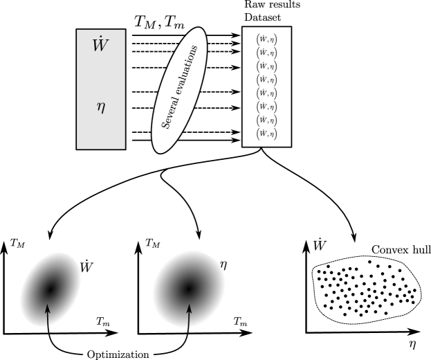
Figure 4: Working framework implemented in Python. Top center: for a fixed set of parameters $r_{\Delta s}$, $\gamma$, $\epsilon$, $T_{c}$, $T_{h}$, $\alpha$, $K_{h}$, $K_{l}$, $K_{c}$ and $K_{\text{reg}}$, several evaluations of $\dot{W}$ and $\eta$, using equations (42) and (43) respectively, are done with different values of $T_{M}$ and $T_{m}$, or conversely of $\Delta$ and $\theta$. Bottom left: once these values are obtained, maximum power and efficiency can be computed, each corresponding to a specific values of $(T_{M},T_{m})$ or $(\Delta,\theta)$, as presented in Figure 6. Bottom right: finally, both couples of values $(\eta,\dot{W})$ are used to draw the “power vs. efficiency” curve, thanks to the convex hull algorithm, as presented in Figure 7.

4.2 Convex hull algorithm

Obtaining the long-awaited power vs. efficiency curve, like the one presented in Figure 7, requires to compute the convex hull (or convex envelope) of a set of points. The convex hull could be defined as the minimal set of points that will define a polygon which includes all the points of the initial set. With a large number of points (around $2150$ in our case) the convex hull is computed thanks to the Graham’s algorithm [69, 70]. This algorithm can be described as follow:

1. Find the center of gravity, noted $G$ of the initial set of points.

2. Compute the counterclockwise angle from $G$ to all other points of the set.

3. Sort the points by angle.

4. Construct the boundary by scanning the points in the sorted order and performing only “right turns” (trim off “left turns”).

To explain the Graham’s scan algorithm, the Figure 5-a presents a simpler example with a small dataset of $15$ points.

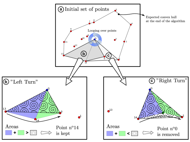
Figure 5: Graham’s scan algorithm, used in this paper to compute power vs. efficiency curve of the model, applied to a simpler example of a set of $15$ points. Top center: once the position of the center of gravity $G$ is known, the counterclockwise angles from $G$ to all these points are calculated and sorted. Thus, thanks to comparisons of triangles surfaces, a point is either kept as a member of the set enveloppe (bottom left) or rejected from the latter (bottom right).

The goal is the determination of a “right turn” or “left turn”. As shown by figure 5-b. A “left turn” can be determined by comparing the areas of several triangles. For a set of 3 points, #13, #14 and #0 in Figure 5-b for example, plus the center of gravity $G$, let’s consider 3 triangles ($G-13-14$, $G-14-0$ and $G-13-0$) and their respective areas.

If the sum of the surfaces of $G-13-14$ and $G-14-0$ is larger than the surface of $G-13-0$: the point $14$ is outside, or in terms of directions, the path $13-14-0$ makes a “left turn”. The rejection of a point, #0 in Figure 5-c, is decided when a “right turn” is detected. This procedure need to be repeated over all the points, in a counterclockwise manner, to ensure the convergence.

For a large dataset of about $2150$ points like the one presented in Figure 7, the Graham’s scan algorithm could be easily parallelized by splitting the original dataset. Each processor will deal with a subset of the original data and a convex hull will be determined for each subset. By merging the different convex hulls a smaller dataset is obtained on which the algorithm is applied. The final convex hull will represent the “power vs. efficiency” curve.

5 Results

At first, a reference case is considered, with a net power $\dot{W}$ and an efficiency $\eta$ which are functions of the maximum and minimum working gas temperatures $T_{M}$ and $T_{m}$, or conversely of $\Delta$ and $\theta$ and with a fixed set of parameters $r_{\Delta s}$, $\gamma$, $\epsilon$, $T_{c}$, $T_{h}$, $\alpha$, $K_{h}$, $K_{l}$, $K_{c}$ and $K_{\text{reg}}$.

Therefore, optimal temperatures that provided maximum power and efficiency are determined and secondly an exhaustive investigation of the impact of $5$ parameters, i.e. $\left(\alpha,K_{l},K_{c},K_{h},K_{\text{reg}}\right)$ for a large range of working gas temperatures is performed.

5.1 Reference case

Table 1: Fixed and adjustable parameters for equations (42) and (43). This particular set of parameters is used to obtain Figures 6 and 7.

	$r_{\Delta s}$	$\gamma$	$\epsilon$	$T_{c}$	$T_{h}$
Fixed	-	-	-	$\mathrm{K}$	$\mathrm{K}$
	1.05	1.4	2	300	1000
	$\alpha$	$K_{h}$	$K_{c}$	$K_{l}$	$K_{\text{reg}}$
Adjustable	-	$\mathrm{W\cdot K^{-1}}$	$\mathrm{W\cdot K^{-1}}$	$\mathrm{W\cdot K^{-1}}$	$\mathrm{W\cdot K^{-1}}$
	0.5005	3000	3000	250	10000

Although many Stirling engines use different working gases, helium was used in our study to maintain compatibility with existing standard cycle calculations. The compression ratio $\epsilon$ and the mass flow was held constant during the cycle. The gas constant for helium is supposed constant at $r=2080\,\mathrm{J\cdot kg^{-1}\cdot K^{-1}}$. The entropic parameter $r_{\Delta s}$ is set to $1.05$. The sink temperature $T_{c}$ is chosen to be at $300\,{\rm K}$ and the hot source temperature $T_{h}$ at $1000\,{\rm K}$. These values are summarized in Table 1.

Hence, for this case the working gas temperatures $\left(T_{M},T_{m}\right)$ will be considered to be adjustable within the range $\left|T_{h}-T_{c}\right|$. For the regenerator effectiveness $\alpha$ and the thermal conductance $K_{i}$, see the lower part of Table 1.

The surfaces of response obtained thanks to such calculation are presented in Figure 6.

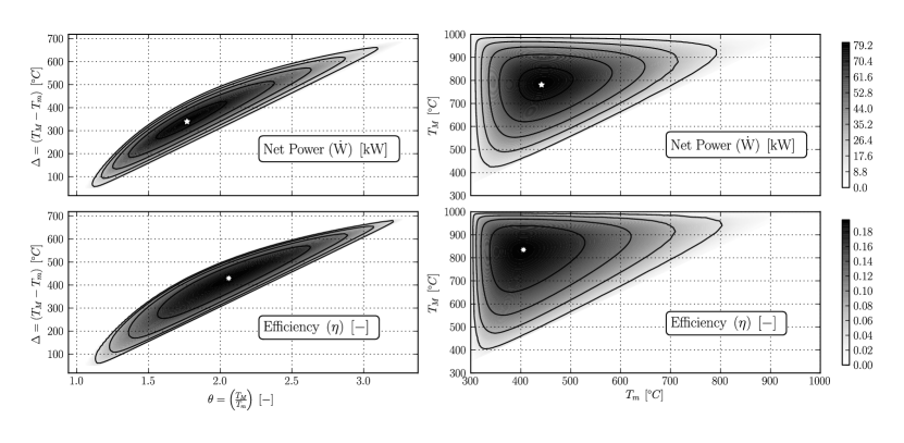
Figure 6: Net power $\dot{W}$ and efficiency $\eta$ as a function of $(\theta,\Delta)$ or $(T_{M},T_{m})$ with the parameters presented in Table 1. The star symbols indicate the optimum $(\bigstar,*)$.

The power of equation (42) and the thermal efficiency of equation (43), respectively presented on the higher and lower parts of Figure 6, are computed regarding to the couple of temperatures $(T_{M},T_{m})$ on the right part of the same figure, and to the parameters $(\Delta,\theta)$ on its left part. For both $\dot{W}$ and $\eta$, an optimum couple of parameters — $(T_{M},T_{m})$ and $(\Delta,\theta)$ — is obtained and drawn, respectively by a symbol $\bigstar$ and $*$.

Once drawn on the $(\eta,\dot{W})$ plan, the same results gives the “power vs. efficiency” curve of Figure 7, on which the maximum net power $\dot{W}_{\max}$ noted by $\bigstar$ and the maximum efficiency $\eta_{\max}$ noted by $*$ are represented.

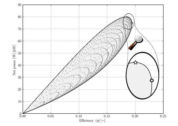
Figure 7: Net power $\dot{W}$ vs. efficiency $\eta$ curve with the parameters of Table 1. The symbol $\bigstar$ indicates the maximum power $\dot{W}_{\max}$ while the symbol $*$ indicates the maximum efficiency $\eta_{\max}$. Numerical values of these optimal parameters are presented in Table 2.

The corresponding temperatures $T_{m}$ and $T_{M}$ are listed in Table 2.

Table 2: Optimal values of the working gas temperature for the reference case, and the resulting maximum power and efficiency.

		Optimum	$T_{m}$	$T_{M}$
$\dot{W}_{\max}$	$\bigstar$	80 kW	442 K	781 K
$\eta_{\max}$	$*$	0.194	405 K	835 K

In terms of temperature, the optimal region is obtained by maintaining the cold and the hot part of the engine in a narrow range of $\sim 50\,{\rm K}$ with a mean value at $T_{m}=423\,{\rm K}$ for the cold side, and with $T_{M}=808\,{\rm K}$ for the hot side.

5.2 Parametric study

A parametric study is conducted in order to observe the effect of the thermal conductances $K_{h}$, $K_{c}$ and $K_{l}$, and of the regenerator conductance $K_{\text{reg}}$ and effectiveness $\alpha$ on the values of both maximal power and maximal efficiency previously obtained on the reference case. For this study, the fixed parameters remain at their previous values presented in Table 1 while the adjustable ones may vary in ranges presented in Table 3.

Table 3: Variation ranges considered for the parametric study. Each parameter is evaluated 17 times within his own range.

	$\alpha$	$K_{h}$	$K_{c}$	$K_{l}$	$K_{\text{reg}}$
	-	$\mathrm{W.K^{-1}}$	$\mathrm{W.K^{-1}}$	$\mathrm{W.K^{-1}}$	$\mathrm{W.K^{-1}}$
minimum	$10^{-3}$	$10^{3}$	$10^{3}$	$10^{-3}$	$5\cdot 10^{3}$
maximum	$1$	$5\cdot 10^{3}$	$5\cdot 10^{3}$	$5\cdot 10^{2}$	$15\cdot 10^{3}$

The variation range of each parameter could be seen as wide at first glance, but it has been chosen to enhance a noticeable change on the net power and efficiency.

For each set of parameters $\alpha$, $K_{h}$, $K_{l}$, $K_{c}$ and $K_{\text{reg}}$, the same as procedure as the reference case is followed:

• Investigation over $T_{m}$ and $T_{M}$ to obtain a similar result as the previous one presented in Figure 6 and Figure 7.

• Numerical optimization to determine the maximum power $\dot{W}_{\max}$ and the maximum efficiency $\eta_{\max}$.

• Each optimum result is characterized by a specific couple of temperatures $T_{m,\text{opt}}$ and $T_{M,\text{opt}}$.

A large amount of data has been processed. With 17 levels for each parameter the total number of cases is $17^{5}\sim 1.4\cdot 10^{6}$. All the combinations and the associate calculations were done, but in the present study only the impact of one parameter at a time is presented, while the others remain at their reference values presented in Table 1.

In Figures 9 and 9, one could observe the influence of each parameter on the optimal net power and on the optimal efficiency, respectively.

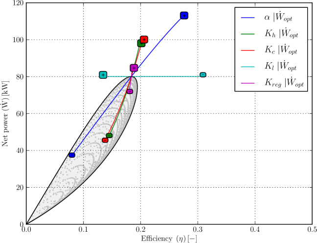
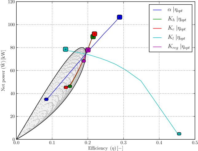
Figure 8: Impact of $\alpha$, $K_{l}$, $K_{c}$, $K_{h}$ and $K_{\text{reg}}$ on the optimal net power $\dot{W}_{\text{opt}}$. Each path is marked by a +⃝ and a -⃝ to indicate the lower and higher value of the selected parameter.

Figure 9: Impact of $\alpha$, $K_{l}$, $K_{c}$, $K_{h}$ and $K_{\text{reg}}$ on the optimal efficiency $\eta_{\max}$. Each path is marked by a +⃝ and a -⃝ to indicate the lower and higher value of the selected parameter.

5.2.1 Influence on optimal net power

At first, it can be observed in Figure 9 that an increase of $\alpha$, $K_{c}$, $K_{h}$ or $K_{\text{reg}}$ enhance both the net power and the associated efficiency. By increasing those parameters, the heat exchange that takes place in the engine tends to an ideal behaviour.

Moreover, from Figure 9, the impact of each parameter $\alpha\gg K_{c}\sim K_{h}\gg K_{\text{reg}}$ on the optimal net power can be analyzed. The regenerator effectiveness $\alpha$ seems to be the key parameter to enhance the performances of the engine. The gain in power is about $45\%$ for a perfect regenerator, while the loss is greater than $50\%$ for a low value of $\alpha$.

The influence of thermal conductances $K_{c}$ and $K_{h}$ on the maximum power produced are similar, from $-40\%$ to about $+25\%$. These influences are stronger than the one of the regenerator conductance $K_{\text{reg}}$ which is almost negligible, from $-10\%$ to $+6\%$.

From a technological and economical points of view, we should keep in mind that great values of thermal conductances suppose very large heat transfer areas or very large coefficients of heat exchange. In fact, such configuration would create much more internal and external irreversibilities and would probably be unacceptable for a real Stirling engine.

The increase of the leak conductance $K_{l}$ corresponds to a larger heat leakage from the hot sink to the cold one. Therefore the efficiency drops dramatically — almost divided by 2 — with a constant optimal net power as predicted by equation (42). $\dot{W}$ is thus independent of $K_{l}$. For heat sources of infinite heat reservoirs, the maximum power does not lead the optimal efficiency, as presented in Figure 9.

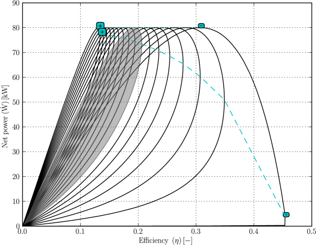
Figure 10: Impact of the leak thermal conductances $K_{l}$ on the convex hull ($-$solid line). Each path is marked by a +⃝ and a -⃝ to indicate the lower and higher value. The dashed line ($--$) corresponds to the change of $K_{l}$ for the optimal net power, same as for Figure 9, and respectively the dotted line ($\cdots$) for the optimal efficiency of Figure 9. The filled grey convex hull is the reference case presented in Figures 7, 9 and 9.

5.2.2 Influence on optimal efficiency

In Figure 9, it can be observed that the parameters $\alpha$, $K_{c}$, $K_{h}$ and $K_{\text{reg}}$ have the same influence on the maximum efficiency $\eta_{\max}$ that they have on the maximum power $\dot{W}_{\max}$, as presented in Figure 9.

About the heat leakage conductance $K_{l}$, the conclusion is not so obvious because an increase of $K_{l}$ both leads to a dramatic loss of the maximum efficiency value and to a relative increase of the net power. The Figure 10 is used for a better understanding of this phenomenon. The “power vs. efficiency” curves are heavily altered by the $K_{l}$ values, going from a lens-shaped curve for high values of $K_{l}$ to a parabolic shaped curve for small values of $K_{l}$. In fact, when $K_{l}$ tends to zero the system tends to the endoreversible engine, as stated in §3.6.2. The opposite case with an increase of $K_{l}$ tends to an Stirling engine which has the ability to produce power but with a very low efficiency. This phenomenon can be explained by the ideal sinks used, of infinite capacities at temperatures $T_{c}$ and $T_{h}$. For any value of $K_{l}$ — even a large one — some heat rate will flow through the Stirling engine. These rates produce a noticeable net power but are negligible in comparaison with the main heat leakage that take place between the hot and cold sink.

6 Conclusion

A thermodynamic analysis of an irreversible realistic Stirling engine model has been carried out and maximum power and maximum efficiency have been obtained numerically in order to provide an estimate of the potential performance bounds for real Stirling engine.

A fully detailed theoretical model is obtained and studied through an innovative method in the Finite Dimension Thermodynamic field. The use of massive computations allows to predict the behaviour of the engine for a large range of its own specific properties. The power and efficiency are easily obtained by using a computational geometry algorithm, the called Graham’s algorithm, that determines the convex hull around the obtained values of the former. This study has shown that the final envelop is fully determined by a set of parameters which are the overall conductances on the hot and cold side and the regenerator properties, i.e. its conductance and effectiveness.

Parametric studies have been conducted with respect to the effect of reservoir temperature, regenerator effectiveness, entropic parameter and reservoir heat conductances. If maximum power and maximum efficiencies increase with the heat source temperature, the different sources of irreversibilities result in a decrease on the performances of the Stirling cycle engine. We demonstrated the key role of the regenerator effectiveness on the performances of the Stirling engine in terms of net power and efficiency. The results of this paper can be used to provide additional insight into the design of irreversible Stirling machine with imperfect regeneration like engines, refrigerators, heat pumps and could be extended to Ericsson machines and any machines with regenerative processes. Additionally the methodology used in this study could be applied in any Finite Dimension Thermodynamic analysis where the analytical expressions are too mathematically complex to be manipulated. Further work should be done to enhance the methodology to be usable to compare the entropy production to the relationship between the maximum power and efficiency and to characterize a dynamic model of a Stirling engine.

Nomenclature

	Notations
$A$	Area, $[{\rm m}^{2}]$
$c_{v}$	Specific heat at constant volume, $[{\rm J\cdot kg}^{-1}\cdot{\rm K}^{-1}]$
$F$	Form factor
$h$	Heat transfer coefficient, $[{\rm W\cdot m}^{-2}\cdot{\rm K}^{-1}]$
$K$	Thermal conductance, $[{\rm W/K}]$
$m$	Mass, $[{\rm kg}]$
$p$	Pressure, $[{\rm bar}]$
$\dot{Q}$	Heat rate, $[{\rm W}]$
$r$	Specific constant of the gas, $[{\rm J\cdot kg}^{-1}\cdot{\rm K}^{-1}]$
$r_{\Delta s}$	Internal irreversibility coefficient
$S$	Entropy, $[{\rm W\cdot K}^{-1}]$
$t$	Time, $[{\rm s}]$
$T$	Temperature, $[{\rm K}]$
$V$	Volume, $[{\rm m}^{3}]$
$\dot{W}$	Mechanical power, $[{\rm W}]$
	Greek symbols
$\alpha$	Regenerator effectiveness
$\Delta$	Difference $T_{M}-T_{m}$
$\epsilon$	Compression ratio of the engine
$\eta$	Energy efficiency
$\theta$	Ratio $T_{M}/T_{m}$.
$\sigma$	Stefan-Boltzmann constant
$\gamma$	Adiabatic index
	Subscripts
$c$	Cold sink
endo	Endoreversible engine
$h$	Hot source
$l$	Heat leak
$m$	Minimum temperature of working gas
$M$	Maximum temperature of working gas
rev	Reversible engine
	Acronyms
FDT	Finite Dimension Thermodynamics
FTT	Finite Time Thermodynamics

References

- Li et al. [2012] T. Li, D. Tang, Z. Li, J. Du, T. Zhou, and Y. Jia. Development and test of a Stirling engine driven by waste gases for the micro-CHP system. Applied thermal engineering, 33-34:119–123, 2012. doi:10.1016/j.applthermaleng.2011.09.020.
- Creyx et al. [2013] M. Creyx, E. Delacourt, C. Morin, B. Desmet, and P. Peultier. Energetic optimization of the performances of a hot air engine for micro-CHP systems working with a Joule or an Ericsson cycle. Energy, 49:229–239, 2013. doi:10.1016/j.energy.2012.10.061.
- Maraver et al. [2013] D. Maraver, A. Sin, J. Royo, and F. Sebastián. Assessment of CCHP systems based on biomass combustion for small-scale applications through a review of the technology and analysis of energy efficiency parameters. Applied Energy, 102:1303–1313, 2013. doi:10.1016/j.apenergy.2012.07.012.
- Kongtragool and Wongwises [2003] B. Kongtragool and S. Wongwises. A review of solar-powered Stirling engines and low temperature differential Stirling engines. Renewable and Sustainable Energy Reviews, 7(2):131–154, 2003. doi:10.1016/S1364-0321(02)00053-9.
- Jokar and Tavakolpour-Saleh [2015] H. Jokar and A. R. Tavakolpour-Saleh. A novel solar-powered active low temperature differential Stirling pump. Renewable Energy, 81:319–337, 2015. doi:10.1016/j.renene.2015.03.041.
- Wang et al. [2016] K. Wang, S. R. Sanders, S. Dubey, F. H. Choo, and F. Duan. Stirling cycle engines for recovering low and moderate temperature heat: A review. Renewable and Sustainable Energy Reviews, 62:89–108, 2016. doi:10.1016/j.rser.2016.04.031.
- Rokni [2013] M. Rokni. Thermodynamic analysis of SOFC (solid oxide fuel cell)–Stirling hybrid plants using alternative fuels. Energy, 61:87–97, 2013. doi:10.1016/j.energy.2013.06.001.
- Gay et al. [2010] C. Gay, D. Hissel, F. Lanzetta, M.-C. Pera, and M. Feidt. Energetic Macroscopic Representation of a Solid Oxide Fuel Cell for Stirling Engine combined cycle in high-efficient powertrains. In IEEE Vehicle Power and Propulsion Conference (VPPC), pages 1–8, Lille, France, September 2010. doi:10.1109/VPPC.2010.5729026.
- Daub [1974] E. E. Daub. The regenerator principle in the Stirling and Ericsson hot air engines. The British Journal for the History of Science, 7(3):259–277, 1974. doi:10.1017/S0007087400013431.
- Dyson et al. [2004] R. W. Dyson, S. D. Wilson, and R. C. Tew. Review of Computational Stirling Analysis Methods. volume 1, pages 511–531, Providence, Rhode Island, August 2004. International Energy Conversion Engineering Conference (IECEC). doi:10.2514/6.2004-5582.
- Touré and Stouffs [2014] A. Touré and P. Stouffs. Modeling of the Ericsson engine. Energy, 76:445–452, 2014. doi:10.1016/j.energy.2014.08.030.
- Chen et al. [1999] L. Chen, C. Wu, and F. Sun. Finite time thermodynamic optimization or entropy generation minimization of energy systems. Journal of Non-Equilibrium Thermodynamics, 24(4):327–359, 1999. doi:10.1515/JNETDY.1999.020.
- Bejan [1996a] A. Bejan. Entropy generation minimization : The new thermodynamics of finite-size devices and finite-time processes. Journal of Applied Physics, 79(3):1191–1218, 1996a. doi:10.1063/1.362674.
- Novikov [1958] I. I. Novikov. The efficiency of atomic power stations. Journal of Nuclear Energy, 7(2):125–128, 1958.
- De Vos [1995] Alexis De Vos. Endoreversible thermoeconomics. Energy conversion and management, 36(1):1–5, 1995. doi:10.1016/0196-8904(94)00040-7.
- Bejan [1996b] A. Bejan. Notes on the History of the Method of Entropy Generation Minimization (Finite Time Thermodynamics). Journal of Non-Equilibrium Thermodynamics, 21(3):239–242, 1996b. doi:10.1515/jnet.1996.21.3.239.
- Vaudrey et al. [2014] A. Vaudrey, F. Lanzetta, and M. Feidt. H. B. Reitlinger and the origins of the efficiency at maximum power formula for heat engines. Journal of Non-Equilibrium Thermodynamics, 39(4):199–203, 2014. doi:10.1515/jnet-2014-0018.
- Curzon and Ahlborn [1975] F. L. Curzon and B. Ahlborn. Efficiency of a Carnot engine at maximum power output. American Journal of Physics, 43:22–24, 1975. doi:10.1119/1.10023.
- Radcenco et al. [1993] V. Radcenco, G. Popescu, V. Apostol, and M. Feidt. Thermodynamique en temps fini appliquée aux machines motrices – Etudes de cas: machine à vapeur et moteur de Stirling. Revue Générale de Thermique, 32(382):509–514, 1993.
- Blank et al. [1994] D. A. Blank, G. W. Davis, and C. Wu. Power Optimization of an Endoreversible Stirling Cycle with Regeneration. Energy, 19(1):125–133, 1994. doi:10.1016/0360-5442(94)90111-2.
- Blank and Wu [1994] D. A. Blank and C. Wu. Power potential of a terrestrial solar-radiant Stirling heat engine. International Journal of Ambient Energy, 15(3):131–139, 1994. doi:10.1080/01430750.1994.9675645.
- Popescu et al. [1996] G. Popescu, V. Radcenco, M. Costa, and M. Feidt. Optimisation thermodynamique en temps fini du moteur de Stirling endo- et exo-irréversible. Revue Générale de Thermique, 35(418-19):656–661, 1996. doi:10.1016/S0035-3159(96)80062-6.
- Ladas and Ibrahim [1994] H. G. Ladas and O. M. Ibrahim. Finite-time view of the Stirling engine. Energy, 19(8):837–843, 1994. doi:10.1016/0360-5442(94)90036-1.
- Senft [1993] J. R. Senft. General Analysis of the Mechanical Efficiency of Reciprocating Heat Engines. Journal of the Franklin Institute, 330(5):967–984, 1993. doi:10.1016/0016-0032(93)90088-C.
- Senft [1998] J. R. Senft. Theoretical limits on the performance of Stirling engines. International journal of energy research, 22(11):991–1000, 1998. doi:10.1002/(SICI)1099-114X(199809)22:11<991::AID-ER427>3.0.CO;2-U.
- Blank [1998] D. A. Blank. Universal power optimized work for reciprocating internally reversible Stirling-like heat engine cycles with regeneration and linear external heat transfer. Journal of Applied Physics, 84(5):2385–2392, 1998. doi:10.1063/1.368364.
- Costea et al. [1999] M. Costea, S. Petrescu, and C. Harman. The effect of irreversibilities on solar Stirling engine cycle performance. Energy conversion and management, 40(15):1723–1731, 1999. doi:10.1016/S0196-8904(99)00065-5.
- Berrin Erbay and Yavuz [1999] L. Berrin Erbay and H. Yavuz. Optimization of the irreversible Stirling heat engine. International Journal of Energy Research, 23(10):863–873, 1999. doi:10.1002/(SICI)1099-114X(199908)23:10<863::AID-ER523>3.0.CO;2-8.
- Kongtragool and Wongwises [2006] B. Kongtragool and S. Wongwises. Thermodynamic analysis of a Stirling engine including dead volumes of hot space, cold space and regenerator. Renewable Energy, 31(3):345–359, 2006. doi:10.1016/j.renene.2005.03.012.
- Rochelle and Grosu [2011] P. Rochelle and L. Grosu. Analytical Solutions and Optimization of the Exo-Irreversible Schmidt Cycle with Imperfect Regeneration for the 3 Classical Types of Stirling Engine. Oil & Gas Science and Technology, 66(5):747–758, 2011. doi:10.2516/ogst/2011127.
- Sigel and Howell [1992] R. Sigel and J. R. Howell. Thermal Radiation Heat Transfer. Hemisphere Publishing Corp., New-York, 1992.
- O’Sullivan [1990] C. T. O’Sullivan. Newton’s law of cooling–a critical assessment. American Journal of Physics, 58(12):956–960, 1990. doi:10.1119/1.16250.
- Angulo-Brown and Páez-Hernández [1993] F. Angulo-Brown and R. Páez-Hernández. Endoreversible thermal cycle with a nonlinear heat transfer law. Journal of applied physics, 74(4):2216–2219, 1993. doi:10.1063/1.354728.
- Reader and Hooper [1983] G. T. Reader and C. Hooper. Stirling Engines. E. & FN Spon, 1983.
- Walker et al. [1993] G. Walker, G. Reader, O. R. Fauvel, and E. R Bingham. The Stirling alternative. Power systems, refrigerants and heat pumps. Gordon and Breach Science Publishers, Inc., New York, United States, 1993.
- Organ [1992] A. J. Organ. Thermodynamics & Gas Dynamics of the Stirling Cycle Machine. Cambridge University Press, 1992.
- Tlili [2012] I. Tlili. Finite time thermodynamic evaluation of endoreversible Stirling heat engine at maximum power conditions. Renewable and Sustainable Energy Reviews, 16(4):2234–2241, 2012. doi:10.1016/j.rser.2012.01.022.
- Shah and Sekulić [2003] R. K. Shah and D. P. Sekulić. Fundamentals of Heat Exchanger Design. John Wiley & Sons, 2003.
- Blank and Wu [1996] D. A. Blank and C. Wu. Power limit of an endoreversible ericsson cycle with regeneration. Energy Conversion and Management, 37(1):59–66, 1996. doi:10.1016/0196-8904(95)00020-E.
- Blank and Bhattacharyya [1999] D. A. Blank and S. Bhattacharyya. Recent advances in finite time thermodynamics, chapter Heating rate limit and cooling rate limit of a reversed reciprocating Stirling cycle., pages 87–103. Nova Science Publishers, New-York, 1999.
- Wu et al. [1998] F. Wu, L. Chen, C. Wu, and F. Sun. Optimum performance of irreversible stirling engine with imperfect regeneration. Energy Conversion and Management, 39(8):727–732, 1998. doi:10.1016/S0196-8904(97)10036-X.
- Lanzetta et al. [1996] F. Lanzetta, P. Nika, and P. K. Panday. étude du transfert de chaleur instationnaire fluide/paroi dans un volume soumis à des variations de pressions cycliques. In Congrès de la Société Française de Thermique, Valenciennes France, 13-15 mai 1996. Société Française de Thermique.
- Nika and Lanzetta [1997] P. Nika and F. Lanzetta. Evaluation pratique des performances d’une machine stirling de taille réduite fonctionnant en cycle frigorifique. Journal de Physique III, 7(7):1571–1591, 1997. doi:10.1051/jp3:1997209.
- Nika and Lanzetta [1995] P. Nika and F. Lanzetta. Développement d’une machine frigorifique Stirling de petite taille adaptée à des niveaux thermiques modérés. Journal de Physique III, 5(5):835–861, 1995. doi:10.1051/jp3:1995164.
- Bejan [1988] A. Bejan. Theory of heat transfer-irreversible power plants. International Journal of Heat and Mass Transfer, 31(6):1211–1219, 1988. doi:10.1016/0017-9310(88)90064-6.
- Chen [1994] J. Chen. The maximum power output and maximum efficiency of an irreversible carnot heat engine. Journal of Physics D: Applied Physics, 27:1144–1149, 1994. doi:10.1088/0022-3727/27/6/011.
- Kodal et al. [2000] A. Kodal, B. Sahin, and T. Yilmaz. A comparative performance analysis of irreversible carnot heat engines under maximum power density and maximum power conditions. Energy Conversion and Management, 41(3):235–248, 2000. doi:10.1016/S0196-8904(99)00107-7.
- Chen et al. [1997] L. Chen, F. Sun, C. Wu, and R. L. Kiang. A generalized model of a real refrigerator and its performance. Applied Thermal Engineering, 17(4):401–412, 1997. doi:10.1016/S1359-4311(96)00043-9.
- Ozkaynak et al. [1994] S. Ozkaynak, S. Gokun, and H. Yavuz. Finite-time thermodynamic analysis of a radiative heat engine with internal irreversibility. Journal of Physics D: Applied Physics, 27:1139–1143, 1994. doi:10.1088/0022-3727/27/6/010.
- Wu and Kiang [1992] C. Wu and R. L. Kiang. Finite-time thermodynamic analysis of a Carnot engine with internal irreversibility. Energy, 17(12):1173–1178, 1992. doi:10.1016/0360-5442(92)90006-L.
- Yan and Chen [1995] Z. Yan and L. Chen. The fundamental optimal relation and the bounds of power output and efficiency for an irreversible Carnot engine. Journal of Physics A: Mathematical and General, 28:6167–6175, 1995. doi:10.1088/0305-4470/28/21/019.
- Kaushik and Kumar [2000] S. C. Kaushik and S. Kumar. Finite time thermodynamic analysis of endoreversible Stirling heat engine with regenerative losses. Energy, 25(10):989–1003, 2000. doi:10.1016/S0360-5442(00)00023-2.
- Kaushik and Kumar [2001] S. C. Kaushik and S. Kumar. Finite time thermodynamic evaluation of irreversible Ericsson and Stirling heat engines. Energy Conversion and Management, 42(3):295–312, 2001. doi:10.1016/S0196-8904(00)00063-7.
- Yaqi et al. [2011] L. Yaqi, H. Yaling, and W. Weiwei. Optimization of solar-powered Stirling heat engine with finite-time thermodynamics. Renewable Energy, 36(1):421–427, 2011. doi:10.1016/j.renene.2010.06.037.
- Chambadal [1957] P. Chambadal. Les centrales nucléaires. A. Colin, 1957.
- Chen et al. [2001] J. Chen, Z. Yan, G. Lin, and B. Andresen. On the curzon-ahlborn efficiency and its connection with the efficiencies of real heat engines. Energy Conversion and Management, 42(2):173–181, 2001. doi:10.1016/S0196-8904(00)00055-8.
- Ahmadi et al. [2015] M. A. Ahmadi, M. A. Ahmadi, Bayat R., M. Ashouri, and M. Feidt. Thermo-economic optimization of Stirling heat pump by using non-dominated sorting genetic algorithm. Energy Conversion and Management, 91:315–322, 2015. doi:10.1016/j.enconman.2014.12.006.
- Toghyani et al. [2014] S. Toghyani, A. Kasaeian, S. H. Hashemabadi, and M. Salimi. Multi-objective optimization of GPU3 Stirling engine using third order analysis. Energy Conversion and Management, 87:521–529, 2014. doi:10.1016/j.enconman.2014.06.066.
- Ahmadi et al. [2013a] M. H. Ahmadi, H. Hosseinzade, H. Sayyaadi, A. H. Mohammadi, and F. Kimiaghalam. Application of the multi-objective optimization method for designing a powered Stirling heat engine: Design with maximized power, thermal efficiency and minimized pressure loss. Renewable Energy, 60:313–322, 2013a. doi:10.1016/j.renene.2013.05.005.
- Ahmadi et al. [2013b] M. H. Ahmadi, H. Sayyaadi, A. H. Mohammadi, and M. A. Barranco-Jimenez. Thermo-economic multi-objective optimization of solar dish-Stirling engine by implementing evolutionary algorithm. Energy Conversion and Management, 73:370–380, 2013b. doi:10.1016/j.enconman.2013.05.031.
- Duan et al. [2014] C. Duan, X. Wang, S. Shu, C. Jing, and H. Chang. Thermodynamic design of Stirling engine using multi-objective particle swarm optimization algorithm. Energy Conversion and Management, 84:88–96, 2014. doi:10.1016/j.enconman.2014.04.003.
- Bert et al. [2014] J. Bert, D. Chrenko, T. Sophy, L. Le Moyne, and F. Sirot. Simulation, experimental validation and kinematic optimization of a Stirling engine using air and helium. Energy, 78(0):701–712, 2014. doi:10.1016/j.energy.2014.10.061.
- Oliphant [2006] T. E. Oliphant. Guide to NumPy, March 2006. URL http://www.tramy.us/.
- Dubois and Konrad H.and Hugunin [1996] P. F. Dubois and J. Konrad H.and Hugunin. Numerical python. Computers in Physics, 10(3), May/June 1996.
- Ascher et al. [1999] D. Ascher, P. F. Dubois, K. Hinsen, J. Hugunin, and T. Oliphant. Numerical Python. Lawrence Livermore National Laboratory, Livermore, CA, ucrl-ma-128569 edition, 1999.
- Jones et al. [2001] E. Jones, T. Oliphant, P. Peterson, et al. SciPy: Open source scientific tools for Python, 2001. URL http://www.scipy.org/.
- Hunter [2007] J. D. Hunter. Matplotlib: A 2d graphics environment. Computing in Science & Engineering, 9(3):90–95, May-Jun 2007. doi:10.1109/MCSE.2007.55.
- Kroshko et al. [2008] D. L. Kroshko et al. Openopt, 2008. URL http://openopt.org.
- Graham [1972] R. L. Graham. An efficient algorith for determining the convex hull of a finite planar set. Information processing letters, 1(4):132–133, 1972. doi:10.1016/0020-0190(72)90045-2.
- de Berg et al. [2000] M. de Berg, M. van Kreveld, M. Overmars, and O. Schwarzkopf. Computational Geometry. Algorithms and Applications. Springer, 2000.