A new proposal for diphoton resonance from $E_{6}$ motivated
extra $U(1)$

Abstract

We propose that the diphoton resonance signal indicated by the recent LHC data might also arise from the pair productions of vector-like heavy down-type quarks with mass around $750$ GeV and above. The vector-like quark decays into an ordinary light quark and a Standard Model singlet scalar. The subsequent decay of scalar singlet produces the diphoton excess. Both the vector-like quark and singlet scalars appear naturally in the $E_{6}$, and their masses can be in the TeV scale with a suitable choice of symmetry breaking pattern. The prediction of such a proposal would be to see an accompanying dijet signal at the same mass with similar cross section in the $2\gamma+2j$ final state and two dijet resonances at the same mass for a $4j$ final state with a cross section, about 100 times larger. Both predictions can be tested easily as the luminosity accumulates in the upcoming runs of the LHC.

I Introduction

Recent observation of diphoton excess at $750$ GeV is the only tentative new physics at the LHC so far atlas ; CMS:2015dxe . This observation is reinforced when combined with data of the early $13$ TeV run with that of events collected at $8$ TeV, though the significance is not large enough to claim any discovery Aaboud:2016tru ; CMS:2016owr . The diphoton excess cross section is in the range of $3-10$ femtobarns (fb), with a resonance width which can be small (around a GeV) or large (around $45$ GeV).

A significant number of papers have proposed a solution by assuming the gauge extensions of the Standard Model (SM) symmetry U1extensions ; gauge_ext which results in the required new particle set that can fit the diphoton excess. A large number of these papers have a model with TeV-scale breaking $U(1)$ where the scalar and exotic fermions carry non-trivial charges under the new $U(1)$ U1extensions . In most of the works the singlet scalar is produced by two gluons through the vector-like quark triangle loop (similar to the SM Higgs production via the top quark loop). Then the singlet scalar decays into two photons (as well as more dominantly to two gluons) again via the heavy vector-like fermion loops. One drawback of this scenario is that the Yukawa coupling of Q to S, $y_{\bar{Q}QS}$, required is non-perturbative to explain the observed level of cross section, or many copies of such Q’s need to be introduced. In general, this kind of approach explains why the vector-like fermions are around the TeV scale.

In this work, we propose an alternative production mechanism for this observed diphoton excess which can complement the standard production mode mentioned above or have a significant event rate by itself. Our mechanism is that the singlet scalar producing this diphoton signal comes from the decay of a heavy down-type quark $xd$ which is a color triplet and an $SU(2)$ singlet with an electric charge of $-1/3$. This heavy down-type exotic quark is pair produced dominantly from two gluons via strong interactions. There are two things which help us in increasing the cross section. The $xd\,\,\overline{xd}$ pair production cross section is much larger than the singlet scalar production via the $xd$ loop (unless the Yukawa coupling of the scalar is somewhat greater than unity). Also, three such $xd$ and $\overline{xd}$ quarks naturally appear in our model based on $E_{6}$ from three fermion families. The singlet scalar is also naturally present. The pattern of symmetry breaking that we shall use gives the singlet scalar mass which is close to the $xd$-quark mass. The version of $E_{6}$ model that we use will be discussed in the next section.

One thing we want to emphasize is that the vector-like quark and singlet scalar, which we are using to explain the diphoton excess, are not postulated in an ad-hoc manner for this purpose, but these particles are already present in the $E_{6}$ grand unified model. All we do is to use the appropriate symmetry breaking pattern so that one $U(1)$ in addition to the SM gauge symmetry remain unbroken at the TeV scale or even higher. The quantum numbers of all the particles are fixed from the $E_{6}$ symmetry. Because of the underlying $E_{6}$ symmetry, in addition to explaining the diphoton excess, we have several predictions. Along with the diphoton resonant signal, we will also have events which have both the diphoton resonance as well as a dijet resonance with similar level of cross sections. Also we shall have events with two dijet resonance at the same mass but with cross section about 100 times the diphoton resonance. These predictions can be tested as more data accumulates at the upcoming 13 TeV LHC runs.

In section II below, we discuss our model and the formalism. In section III, we discuss the phenomenology of our model. This includes the details of how our model can explain the diphoton excess, and the other predictions that can be tested in near future. Section IV contains our conclusions and discussions.

II The model and the formalism

Our effective symmetry at the TeV scale is the SM together with an extra $U(1)^{\prime}$. This extra $U(1)^{\prime}$ is a special subgroup of the $E_{6}$ Grand Unified Theory (GUT) gursey ; Langacker:2008yv ; general ; PLJW ; Erler:2002pr ; Kang:2004pp ; Kang:2004ix ; Kang:2009rd . We use non-supersymmetric $E_{6}$. $E_{6}$ is special in the sense that it is anomaly free, as well as has chiral fermions. Its fundamental representation reduces under $SO(10)$ as

$$\bf 27=16+10+1$$

The representation 16 contains the $15$ SM fermions, as well as a right handed neutrino. It decomposes under $SU(5)$ as

$$\bf 16=10+\bar{5}+1$$

The 10 representation under $SU(5)$ decomposes as

$$\bf 10=5+\bar{5}+1$$

The 5 contains a color triplet and a $SU(2)_{L}$ doublet, whereas $\bf\bar{5}$ contains a color anti-triplet and another $SU(2)$ doublet, and the $\bf 1$ is a SM singlet. The gauge boson is contained in the adjoint $\bf 78$ representation of $E_{6}$.

The particle content of the $\bf 27$ representation, which contains the SM fermions as well as the extra fermions, are shown in the first two columns of Table 1. For three families of fermions, we use three such $\bf 27$. The $E_{6}$ gauge symmetry can be broken as follows Group ; Hewett:1988xc ,

$$E_{6}\to\ SO(10)\times\ U(1)_{\psi}\to\ SU(5)\times\ U(1)_{\chi}\times\ U(1)_{\psi}~{}.~{}\,$$ (1)

The $U(1)_{\psi}$ and $U(1)_{\chi}$ charges for the $E_{6}$ fundamental ${\bf 27}$ representation are also given in Table 1.

The $U(1)^{\prime}$ is one linear combination of the $U(1)_{\chi}$ and $U(1)_{\psi}$

$$Q^{\prime} = \cos\theta\ Q_{\chi}+\sin\theta\ Q_{\psi}~{}.~{}\,$$ (2)

The other $U(1)$ gauge symmetry from the orthogonal linear combination as well as the $SU(5)$ is broken at a high scale. This will allow us to have a large doublet-triplet splitting scale, which prevents rapid proton decay if the $E_{6}$ Yukawa relations were enforced. This will need either two pairs of (${\bf 27}$, ${\bf{\overline{27}}}$) and one pair of (${\bf 351^{\prime}}$, ${\bf\overline{351^{\prime}}}$) dimensional Higgs representations, or one pair of (${\bf 27}$, ${\bf{\overline{27}}}$), ${\bf 78}$, and one pair of (${\bf 351^{\prime}}$, ${\bf\overline{351^{\prime}}}$) dimensional Higgs representations (Detailed studies of $E_{6}$ theories with broken Yukawa relations can be found in King:2005jy ; Babu:2015psa .) For our model, the unbroken symmetry at the TeV scale is $SU(3)_{C}\times SU(2)_{L}\times U(1)_{Y}\times U(1)^{\prime}$.

$SO(10)$	$SU(5)$	$2\sqrt{10}Q_{\chi}$	$2\sqrt{6}Q_{\psi}$	$4\sqrt{15}Q$
16	$10~{}(Q_{i},U_{i}^{c},E_{i}^{c})$	–1	1	$1$
	${\bar{5}}~{}(D_{i}^{c},L_{i})$	3	1	7
	$1~{}(N_{i}^{c}/T)$	–5	1	$-5$
10	$5~{}(XD_{i},XL_{i}^{c}/H_{u})$	2	–2	$-2$
	${\bar{5}}~{}(XD_{i}^{c},XL_{i}/H_{d})$	–2	–2	$-8$
1	$1~{}(XN_{i}/S)$	0	4	10

Table 1: Decomposition of the $E_{6}$ fundamental ${\bf 27}$ representation under $SO(10)$, $SU(5)$, and the $U(1)_{\chi}$, $U(1)_{\psi}$ and $U(1)^{\prime}$ charges.

We explain our convention in some details as given in Table 1. Our notation is similar to what is used in the supersymmetric case. We have denoted the SM quark doublets, right-handed up-type quarks, right-handed down-type quarks, lepton doublets, right-handed charged leptons, and right-handed neutrinos as $Q_{i}$, $U_{i}^{c}$, $D_{i}^{c}$, $L_{i}$, $E_{i}^{c}$, and $N_{i}^{c}$, respectively. Second, in our model, we introduce three fermionic ${\bf 27}$s, one scalar Higgs doublet field $H_{u}$ from the doublet of ${\bf{5}}$ of $SU(5)$, one scalar Higgs doublet field $H_{d}$ from the doublet of ${\bf{\bar{5}}}$ of $SU(5)$, one scalar SM singlet Higgs field $T$ from the singlet of ${\bf 16}$ of $SO(10)$, and one scalar SM singlet Higgs field $S$ from the singlet of ${\bf 27}$ of $E_{6}$. Thus, similar to the fermions, all the scalars with mass in the TeV scale are coming from the ${\bf 27}$ of $E_{6}$. Note that the additional fermions from the ${\bf 27}$ with masses at the TeV scale are $N_{i}^{c}$, $XD_{i}$, $XL_{i}^{c}$, $XD_{i}^{c}$, $XL_{i}$, and $XN_{i}$. For details, please see Table 2.

In our model, the $S$ gives the Majorana mass to the right-handed neutrinos $N^{c}_{i}$ after $U(1)^{\prime}$ gauge symmetry breaking, i.e., the terms $SN_{i}^{c}N_{i}^{c}$ are $U(1)^{\prime}$ gauge invariant. The mixing angle in our model is given by

$$\tan\theta=\sqrt{5/3}~{}.~{}\,$$ (3)

$Q_{i}$	$(\mathbf{3},\mathbf{2},\mathbf{1/6},\mathbf{1})$	$U_{i}^{c}$	$(\mathbf{\overline{3}},\mathbf{1},\mathbf{-2/3},\mathbf{1})$	$D_{i}^{c}$	$(\mathbf{\overline{3}},\mathbf{1},\mathbf{1/3},\mathbf{7})$
$L_{i}$	$(\mathbf{1},\mathbf{2},\mathbf{-1/2},\mathbf{7})$	$E_{i}^{c}$	$(\mathbf{1},\mathbf{1},\mathbf{1},\mathbf{1})$	$N_{i}^{c}/T$	$(\mathbf{1},\mathbf{1},\mathbf{0},\mathbf{-5})$
$XD_{i}$	$(\mathbf{3},\mathbf{1},\mathbf{-1/3},\mathbf{-2})$	$XL^{c}_{i},~{}H_{u}$	$(\mathbf{1},\mathbf{2},\mathbf{1/2},\mathbf{-2})$	$XD_{i}^{c}$	$(\mathbf{\overline{3}},\mathbf{1},\mathbf{1/3},\mathbf{-8})$
$XL_{i},~{}H_{d}$	$(\mathbf{1},\mathbf{2},\mathbf{-1/2},\mathbf{-8})$	$XN_{i},~{}S$	$(\mathbf{1},\mathbf{1},\mathbf{0},\mathbf{10})$

Table 2: The particles and their quantum numbers under the $SU(3)_{C}\times SU(2)_{L}\times U(1)_{Y}\times U(1)^{\prime}$ gauge symmetry. Here, the correct $U(1)^{\prime}$ charges are the $U(1)^{\prime}$ charges in the Table divided by $4{\sqrt{15}}$.

The Higgs potential needed for our purpose giving rise to the extra $U(1)$ symmetry breaking is

$$V=-m_{S}^{2}|S|^{2}-m_{T}^{2}|T|^{2}+\lambda_{S}|S|^{4}+\lambda_{T}|T|^{4}+\lambda_{ST}|S|^{2}|T|^{2}+(\sigma ST^{2}+H.C.)~{}.~{}\,$$ (4)

Note that without the term $\sigma ST^{2}$, there are two global $U(1)$ symmetries for the complex phases of $S$ and $T$. After $S$ and $T$ obtain the Vacuum Expectation Values (VEVs), we have two Goldstone bosons, and one of them is eaten by the extra $U(1)$ gauge boson. Thus, to avoid the extra Goldstone boson, we need the term $\sigma ST^{2}$ to break one global symmetry. Then we are left with only one global symmetry in the above potential, which is the extra $U(1)^{\prime}$ gauge symmetry. Thus, after $S$ and $T$ acquire the VEVs, the $U(1)^{\prime}$ gauge symmetry is broken, and $S$ and $T$ will be mixed via the $\lambda_{ST}|S|^{2}|T|^{2}$ and $\sigma ST^{2}$ terms.

The Yukawa couplings in our models are

$$-{\cal L} = y_{ij}^{U}Q_{i}U_{j}^{c}H_{u}+y_{ij}^{D}Q_{i}D_{j}^{c}H_{d}+y_{ij}^{E}L_{i}E_{j}^{c}H_{d}+y_{ij}^{N}L_{i}N_{j}^{c}H_{u}+y_{ij}^{XNd}XL_{i}^{c}XN_{j}H_{d}$$ (5)

$$+y_{ij}^{XNu}XL_{i}XN_{j}H_{u}+y_{ij}^{TD}D_{i}^{c}XD_{j}{T}+y_{ij}^{TL}XL_{i}^{c}L_{j}{T}$$

$$+y_{ij}^{SD}XD_{i}^{c}XD_{j}S+y_{ij}^{SL}XL_{i}^{c}XL_{j}S+{\rm H.C.}~{},~{}\,$$

where $i=1,~{}2,~{}3$. Thus, after $S$ and $T$ obtain VEVs or after $U(1)^{\prime}$ gauge symmetry breaking, $(XD_{i}^{c},~{}XD_{i})$ and $(XL_{i}^{c},~{}XL_{i})$ will become vector-like particles from the $y_{ij}^{SD}XD_{i}^{c}XD_{j}S$ and $y_{ij}^{SL}XL_{i}^{c}XL_{j}S$ terms, and $(D_{i}^{c},~{}XD_{i})$ and $(XL_{i}^{c},~{}L_{i})$ will obtain vector-like masses from the $y_{ij}^{TD}D_{i}^{c}XD_{j}{T}$ and $y_{ij}^{TL}XL_{i}^{c}L_{j}{T}$ terms. For simplicity, we assume $y_{ij}^{SD}\langle S\rangle>>y_{ij}^{TD}\langle{T}\rangle$ and $y_{ij}^{SL}\langle S\rangle>>y_{ij}^{TL}\langle{T}\rangle$. After we diagonalize their mass matrices, we obtain the mixings between $XD_{i}^{c}$ and $D_{i}^{c}$, and the mixings between $XL_{i}$ and $L_{i}$. The discussion of the Higgs potential for electroweak symmetry breaking is similar to the Type II two Higgs doublet model, so we will not repeat it here.

After $U(1)^{\prime}$ gauge symmetry breaking, we obtain two CP-even Higgs fields $s_{h}$ and $t_{h}$, and one CP-odd Higgs field $a_{h}$ by diagonalizing the mass matrices of $S$ and $T$. Thus, we can have one, two, or three 750 GeV resonances of which the most likely candidate would be the $s_{h}$ as it will have the strongest coupling to the vector-like fermions. Although it looks equally probable to have a mixture of any of the aforementioned fields to be the observed resonance in the diphoton mode, there is also the possibility that one can have additional sources for the observed resonance. There is a viable region of the parameter space in our model where the pair production of the vector-like fermions, $(XD_{i}^{c},~{}XD_{i})$, and their subsequent decays to any of the scalars, $s_{h}$, $t_{h}$ or $a_{h}$ will give rise to the diphoton and other observable signals. The phenomenology of the model is discussed in the next section. We note that the supersymmetric $E_{6}$ GUT has also been used in Ref. king , but our model is non-supersymmetric. And more importantly we address an additional mechanism for producing the diphoton excess and associated signals, and therefore the subsequent predictions are entirely different from theirs.

We note that the $U(1)^{\prime}$ gauge boson couples to all the SM fields in addition to the new matter and scalar fields. The covariant derivatives for the $SU(2)_{L}$ doublet and the singlet scalars are given by

$$\begin{split}{\mathcal{D}}_{\mu}&=(\partial_{\mu}-i\frac{\vec{\sigma}}{2}.\vec{W_{\mu}}-ig^{\prime}YB_{\mu}-ig_{X}Y_{X}Z^{\prime}{{}_{\mu}}),\end{split}$$ (6)

where $Y(H_{u})=\frac{1}{2},Y(H_{d})=-\frac{1}{2}$ and $Y_{X}(H_{u})=-\frac{2}{4\sqrt{15}},Y_{X}(H_{d})=-\frac{8}{4\sqrt{15}}$;

$$\begin{split}{\mathcal{D}}_{\mu}&=(\partial_{\mu}-ig_{X}Y_{X}Z^{\prime}{{}_{\mu}}),\end{split}$$ (7)

where $Y_{X}(S)=\frac{10}{4\sqrt{15}}$ and $Y_{X}(T)=-\frac{5}{4\sqrt{15}}$. The mass square matrix for the neutral gauge boson sector in the $(W_{3},B,Z^{\prime})$ basis is then given as

$$\mathcal{M}=\begin{pmatrix}{\Huge({\mathcal{M}_{SM}})_{2\times 2}}&\begin{matrix}\mathcal{M}_{13}\\ \mathcal{M}_{23}\end{matrix}\\ \begin{matrix}\mathcal{M}_{13}&\mathcal{M}_{23}\end{matrix}&\mathcal{M}_{33},\end{pmatrix}$$

where

$$\mathcal{M}_{13}=\frac{gg_{X}}{8\sqrt{15}}(2v_{u}^{2}-8v_{d}^{2}) \mathcal{M}_{23}=-\frac{g^{\prime}g_{X}}{8\sqrt{15}}(2v_{u}^{2}-8v_{d}^{2})~{},$$ ,

$${\rm and} \mathcal{M}_{33}=\frac{g_{X}^{2}}{240}(4v_{u}^{2}+64v_{d}^{2}+25v_{t}^{2}+100v_{s}^{2})~{},$$

where the $v_{i}s$ represent the VEVs of the scalar multiplets. Thus, we can clearly see that the new gauge boson mass is dependent on the VEVs of all the scalars, such that one can choose one singlet VEV to be much smaller than the other and still have a very heavy $Z^{\prime}$ that evades the existing limits. Moreover, the mixings between $W_{3}/B$ and $Z^{\prime}$ will be zero at tree level if $v_{u}=2v_{d}$.

The VEVs of the $SU(2)$ doublet scalars determine the SM gauge boson masses and therefore $v_{EW}=\sqrt{v_{d}^{2}+v_{u}^{2}}\simeq 246$ GeV. The structure for the VEVs is given as

$$<H_{d}> =\begin{pmatrix}v_{d}/\sqrt{2}\\ 0\end{pmatrix}~{},~{} <H_{u}> =\begin{pmatrix}0\\ v_{u}/\sqrt{2}\end{pmatrix}~{},~{}$$

$$<T> =v_{t}/\sqrt{2}~{},~{} <S> =v_{s}/\sqrt{2}~{},~{}$$

which leads to the following mass matrix for the down-type quarks and the charged leptons in the $(q_{1},q_{2},q_{3},xq_{1},xq_{2},xq_{3})$ basis is given as

$$\frac{1}{\sqrt{2}}\begin{pmatrix}y_{ij}^{D}v_{d}&0\\ y_{ji}^{TD}v_{t}&y_{ij}^{SD}v_{s}\end{pmatrix}, \frac{1}{\sqrt{2}}\begin{pmatrix}y_{ij}^{E}v_{d}&y_{ji}^{TL}v_{t}\\ 0&y_{ij}^{SL}v_{s}\end{pmatrix},$$ (8)

where $i,j=1,2,3$. The $q_{i}$s and $xq_{i}$s represent the down-type quarks for the left matrix and the leptons for the right matrix. These mass matrices would be diagonalized by a bi-unitary transformation which would lead to a mixing between the vector-like fermions and the SM fermions. However, one should note that the mixings between the left-handed fermions and the right-handed fermions will be dictated by a different set of mixing angles. This would have significant implications in the rest of our analysis and plays a crucial role in the signal we have proposed.

We should also point out a few useful assumptions that we think are relevant for the analysis:

1. We have neglected any mixing between the electroweak doublet scalars and singlet scalars.

2. We also ensure that the new $U(1)^{\prime}$ gauge boson does not have a significant mixing with the SM gauge boson $Z$ ($\mathcal{M}_{13},\mathcal{M}_{23}<<\mathcal{M}_{33}$).

3. The mixings between the left-handed SM fermions and the vector-like fermions are taken to be zero, i.e., we assume the zero left-mixing angle ($\theta_{L}=0$). This will insure that the vector-like fermions do not decay to the SM gauge bosons and light SM fermions Grossmann:2010wm , thus allowing the only significant channel that would be the decay to a scalar ($s_{h},t_{h}$) and SM fermion. One can also get a very suppressed partial width (due to the smallness of the Yuakawa couplings courtesy the masses of the SM down-type quarks and leptons) that decays to a SM Higgs and light SM fermion, through the mixings in the right-handed fermion sector.

III Analysis

The diphoton signal in our model can arise from several possibilities of the particle spectrum as well as in two different production channels. Note that the most popular option in the literature in explaining the diphoton excess has been through the on-shell production of a 750 GeV resonance via gluon fusion which then decays to diphotons. Therefore we must point out that such a possibility clearly exists in our model description. We shall show that what part of the parameter space is best suited for the aforementioned explanation of the diphoton excess and what sort of masses and couplings are required for the new exotics to satisfy the experimental data. Notwithstanding this possibility, we wish to also highlight a new channel of production that can also give rise to the diphoton excess signal and predict an accompanying dijet resonance at the same mass in the same signal events. This would be possible through the pair production of vector-like quarks which is heavier but very close in mass to one of the scalars which has mass of 750 GeV. The pair produced exotic quarks then decay to this 750 GeV scalar and a very soft jet, which is not detected. So we get a pair of these 750 GeV scalars which then decay to either a gluon pair or a diphoton pair. We believe that such a possibility, which exists for a range of the VLQ mass that nearly degenerates with the resonant scalar mass and yet is searched for by the LHC experiments, should show itself with a closer scrutiny of the events along with the new events being collected. We now take up these two possible channels and analyze the diphoton signal for different parameter choices of the model. To calculate the several branching fractions of the new exotic particles and signal cross sections we have used the CalcHEP event generator Belyaev:2012qa . We have implemented the model in LanHEP lanhep to create the model files for CalcHEP.

Note that the analysis will vary depending on the number of vector-like fermions we might possibly have at sub-TeV masses. The colored vector-like fermions participate in both the production channels while the non-colored one’s help in increasing the diphoton branching fraction of the scalar. We shall consider three different scenarios:

• Only one vector-like quark with mass around a TeV while all the remaining vector-like fermions have mass of 1.5 TeV.

• One vector-like quark and one vector-like lepton having TeV mass while the remaining have mass of about 1.5 TeV.

• One vector-like quark and two vector-like degenerate leptons having TeV masses while again the rest of them have mass at 1.5 TeV.

Note that the choice of a fixed scale of 1.5 TeV mass for the vector-like fermions is made as it helps in expressing our results in terms of the singlet scalar VEV of $S$ given by $v_{s}$ which gives the mass to the vector-like fermions as $M_{xd_{i}}=y_{ii}^{SD}v_{s}/\sqrt{2}$ and $M_{x\ell_{i}}=y_{ii}^{SL}v_{s}/\sqrt{2}$. In addition, it helps us in scanning a range for $v_{s}$ such that the perturbative limit of the Yukawa couplings (taken as $y_{ii}/\sqrt{2}<\sqrt{4\pi}$) is not violated. Therefore, a shift in the choice of the mass of the heaviest vector-like fermion would imply that $v_{s}$ can be varied over a different range. This gives us the necessary dynamics to understand how the signal strength gets affected by the choice of the mass of the vector-like fermion.

To study the final states we specify here the parameters that are relevant for the analysis. The vector-like quarks and leptons are represented as $xd_{i}$ and $x\ell_{i}$ respectively. As pointed out earlier, the VEVs for $S$ and $T$ which are given by $v_{s}$ and $v_{t}$ respectively play a significant role in giving mass to the $U(1)^{\prime}$ gauge boson, which we call $Z^{\prime}$. We take the mass of $Z^{\prime}$ to be 1.5 TeV, and fix the value of $v_{t}$ to be 10 TeV. Such large value of $v_{t}$ becomes a necessity to avoid a significant mixing in the neutral gauge boson sector. This also forces very small mixing between the scalars $s_{h}$ and $t_{h}$. This decoupled particle spectrum is somewhat also preferable as the LHC has not observed any other signal other than the diphoton resonance. Note that the new particles in the spectrum can however play a crucial role in determining additional signals for the model at the LHC, which we leave for future analysis as we focus only on the diphoton signal in this work. We consider two types of processes that will contribute to the diphoton production cross section. Note that the experiments have observed a resonance at 750 GeV in the diphoton channel which is best explained by the direct on-shell production in the $s$-channel as shown in Fig. 1. For simplicity, we will take all types of Yukawa couplings $y^{A}_{ij}$ to be zero for $i\neq j$, where $A\equiv TD,TL,SD,SL$ (see Sec. II).

• $pp\rightarrow s_{h}\rightarrow\gamma\gamma$

  

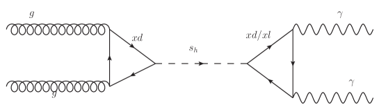
  Figure 1: The Feynman diagram which contributes to the diphoton production through the onshell production of $s_{h}$ as an s-channel resonance via gluon-gluon fusion at the LHC.

  Through out the analysis we shall identify this process as diphoton production through resonant $s_{h}$ channel. The parton level Feynman diagram for this process is shown in Fig. 1 and the cross section is given by $\sigma_{1}=\sigma(pp\rightarrow s_{h})\times Br(s_{h}\rightarrow\gamma\gamma)$.

  

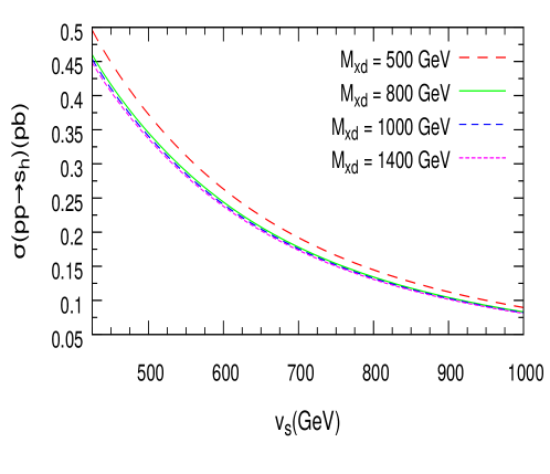
  Figure 2: The s-channel production cross section of $s_{h}$ via the gluon-gluon fusion at LHC with $\sqrt{s}=13$ TeV, as a function of VEV of the singlet $S$; $v_{s}$ for different values of $M_{xd_{1}}$.

  To study the $s_{h}$ production, the relevant parameters are the VLQ mass and the VEV $v_{s}$ which gives the Yukawa strength of the VLQ interaction with the scalar $s_{h}$. The loop induced production of the $s_{h}$ depends on its coupling to the massless gluons which is given by the effective Lagrangian

  $$\mathcal{L}_{sGG}=-\lambda_{sgg}s~{}G_{\mu\nu}G^{\mu\nu}.$$ (9)

  In Eq. 9, $\lambda_{sgg}=\alpha_{s}F_{1/2}(\tau_{xd})/(16\pi v_{s})$ where $F_{1/2}(\tau_{xd})=2(\tau_{xd}+(\tau_{xd}-1)f(\tau_{xd}))\tau_{xd}^{-2}$ represents the loop function and $f(\tau_{xd})=(sin^{-1}\sqrt{\tau_{xd}})^{2}$ with $\tau_{xd}=m_{s_{h}}^{2}/4M_{xd}^{2}$. The $s_{h}$ production cross section depends on the VLQ content only and not on the VLL content. For all the three cases we have considered for our analysis, we choose only one VLQ whose mass is varied while the remaining two have mass of 1.5 TeV. Hence for all the three cases the $s_{h}$ production cross section will be same for a given value of $M_{xd_{1}}$. In Fig. 2 we show the leading-order production cross section of the scalar $s_{h}$ as a function of the VEV $v_{s}$ for different values of the lightest VLQ mass. The lower values of $v_{s}$ imply a large Yukawa coupling invariably leading to larger production cross sections. The cross sections are doubled if one takes a QCD $K$-factor of $\sim 2$ as for the SM Higgs boson. In addition, we note that as the lightest VLQ mass is increased to 1.4 TeV, there does not seem to be a significant fall. This is because in all production curves, there is some contributions from the two heavy VLQ’s with mass 1.5 TeV. Thus, with even three VLQ’s with mass 1.5 TeV, the production cross section can be quite large.

• $pp\rightarrow xd$ $\overline{xd}\rightarrow\gamma\gamma$ + jets

  

  

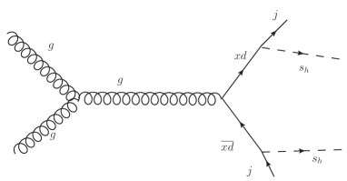
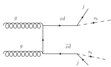
  Figure 3: The Feynman diagrams for the dominant subprocess contributing to the pair production of the VLQ and its subsequent decay to $s_{h}$ and an additional jet ($j$) giving an $s_{h}$ pair and two jets in the final state.

  This is the alternative approach that can also contribute to the events of diphoton excess. Through out the analysis this process is termed as diphoton production through $xd$ pair production channel. The parton level Feynman diagrams for the dominant process are shown in Fig. 3, where we have not shown the diagrams for the $q\bar{q}$ initiated subprocesses.

  Note that the production of the $xd$ pair at LHC is dominantly through the gluon-gluon fusion and in Fig. 4 we plot the total pair production cross section (leading-order) of $xd$ at the LHC with $\sqrt{s}=13$ TeV, as a function of $M_{xd}$ with values between 760-800 GeV. The decay $xd\rightarrow s_{h}\,\,j$ leads to a relatvely soft jet and a pair of the 750 GeV scalar $s_{h}$. The $s_{h}$ can now decay to a pair of photons or gluons. Thus we get a resonant diphoton signal along with multiple jets.

  

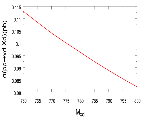
  Figure 4: The pair production cross section of $xd$ at LHC with $\sqrt{s}=13$ TeV, as a function of $M_{xd}$ with values between 760-800 GeV.

  The diphoton cross section in this channel is then given by

  $$\sigma_{2}=2\times\sigma(pp\rightarrow xd,\overline{xd})\times[Br(xd\rightarrow s_{h}\,\,j)]^{2}\times Br(s_{h}\rightarrow\gamma\gamma)\times Br(s_{h}\rightarrow gg).$$

  For our analysis we choose parameters such that $Br(xd\rightarrow s_{h}\,\,j)\simeq 1$ is ensured when $M_{xd}>m_{s_{h}}$. We have already discussed in Sec. II why the other usual decay modes of the VLQ are absent in our model. This also ensures that the mass bounds on the VLQ can be significantly relaxed as the dominant decay of the VLQ when $M_{xd}<m_{s_{h}}$ is $xd\rightarrow h\,\,j$ while $xd\rightarrow s_{h}\,\,j$ when $M_{xd}>m_{s_{h}}$. Note that the decay to the SM gauge bosons will be allowed once we allow the left-handed SM fermions to mix with the VLQ and VLL.

The decay of the scalar into two photons is again dependent on the mass and Yukawa strengths of the vector-like fermions. As the number of light vector-like leptons are not severely constrained by experiments and their inclusion helps in improving the $s_{h}\to\gamma\gamma$ branching fraction, we shall consider the results with one or more of such VLL contributing to the diphoton decay. We plot the branching ratio for the scalar $s_{h}$ decaying into a pair of photons in Fig. 5 as a function of the VLL mass for different values of the lightest VLQ mass. For the branching ratio plot, we have considered two degenerate VLL’s and one light VLQ while the heaviest VLL and VLQ’s have their mass set at 1.5 TeV. Note that including more light VLQ’s would boost the production channel for both the production processes ($pp\to s_{h}$ and $pp\to xd\,\,\overline{xd}$) but reduces the branching fraction of $s_{h}\to\gamma\gamma$ as the partial width of $s_{h}\to gg$ becomes much larger. We therefore now consider the two cases where we have one light VLQ and VLL each, and when we have one light VLQ and two light degenerate VLL’s.

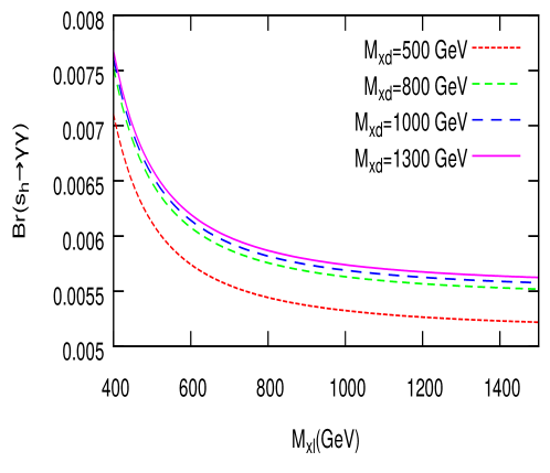
Figure 5: The diphoton branching ratio as a function of the VLL mass for different values of the lightest VLQ mass. The branching ratio is evaluated using two light degenerate VLL’s with mass $M_{x\ell}$ and one light VLQ with mass $M_{xd}$.

III.1 Diphoton signal

We now proceed to analyse the two production channels for the scalar $s_{h}$ and compare the signal strengths into the diphoton mode. Being in the perturbative limit of the Yukawa couplings and by varying parameters $v_{s}$, $M_{xd}$ and $M_{x\ell}$ we shall check the availability of parameter space which keeps the diphoton cross section within 3-10 fb range. The light vector-like leptons have been taken to be degenerate for simplicity. The value of $v_{s}$ has been varied from 425 GeV to 1 TeV with the lower cut-off, dependent on the choice of 1.5 TeV as the mass of the heaviest VLQ/VLL which determines the perturbative limit for the Yukawa couplings. Thus, it is clear that if the mass of the heaviest VLQ is reduced, then a lower $v_{s}$ would be allowed. The $s_{h}$ production cross section decreases with increase in either $M_{xd}$ or $v_{s}$ as shown in Fig.2. This happens because the loop contributions get suppressed for heavier $M_{xd}$ while the Yukawa strength becomes smaller when $v_{s}$ is increased for a fixed $M_{xd}$.

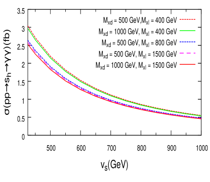
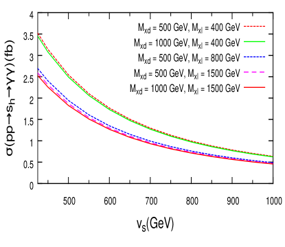
Figure 6: The diphoton production cross section as a function of $v_{s}$ for different choices of $M_{xd}$ and $M_{x\ell}$. The left panel represents (one VLQ, one VLL) while the right-panel represents (one VLQ, two VLL) whose mass is varied. The heavier VLQ/VLL states have a fixed mass of 1.5 TeV.

In Fig. 6 we show the contribution to diphoton cross section from $s_{h}$ resonant production channel as a function of $v_{s}$ for different sets of ($M_{xd}$,$M_{xl}$). Note that the left panel in Fig. 6 corresponds to the case of (one VLQ, one VLL) while the right panel represents (one VLQ, two VLL) whose masses are varied. The curves also represent a variation of the Yukawa coupling which is decreasing from left-to-right and quite clearly, a large value of the coupling is more favorable to generate the correct size of the diphoton signal rate but looks possible even with a VLQ as heavy as 1 TeV and a single light VLL in the spectrum. Note that a reasonable enhancement is possible with appropriate $K$-factors for the production of $s_{h}$. The inclusion of an extra light VLL in the spectrum of similar mass seems to enhance the diphoton rate by about 16% when the VLL’s are in the mass range of 400 GeV, as shown in the right panel of Fig. 6. For the heavier VLL’s the difference is hardly noticeable when compared to the case with one light VLL.

We now consider the diphoton rate expected from the pair production of the VLQ’s having mass which is near degenerate with the 750 GeV scalar $s_{h}$. We assume a range of $M_{xd}=760-800$ GeV to show the inclusive rate for the diphoton signal. In Fig.7 we plot this contribution evaluated at leading-order, to the diphoton signal via $xd$ pair production as a function of $M_{xd}$ being in the range $760-800$ GeV and for different values of $M_{x\ell}$ for the two cases, (one VLQ, one VLL - left panel) and (one VLQ, two VLL - right panel). Again, we must point out here that a reasonable enhancement is expected from appropriate QCD $K$-factors for the $xd$-pair produced through strong interactions. As the production of the VLQ pair as well as its decay are not dependent on the choice of $v_{s}$ or the Yukawa strength, the number of light VLQ’s and light VLL’s are the major players in determining the event rates here. However, the important thing to note here is that with a very degenerate VLQ and $s_{h}$, the contributions to the inclusive diphoton rate is quite significant. In principle, inclusion of more generations of the VLQ should give a much enhanced rate for the inclusive diphoton production in this channel which would be clearly observable in its own individuality.

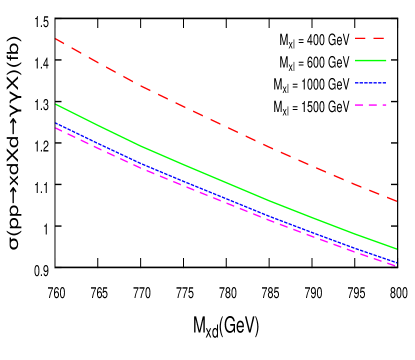
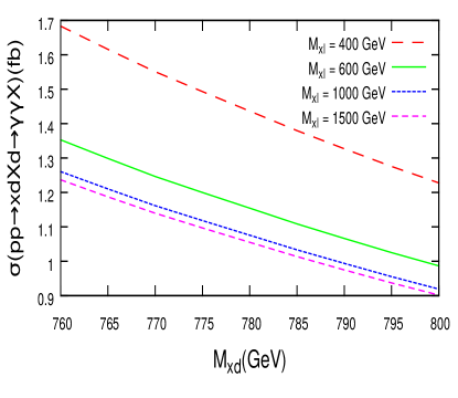
Figure 7: The inclusive diphoton production cross section from $xd$ pair production as a function of $M_{xd}$ for different values of $M_{xl}$. The two panels represent the similar configurations as in Fig. 6.

Thus, this channel would stand to explain the diphoton excess even when the Yukawa couplings are very small and contributions to the diphoton rate via $s_{h}$ resonant production becomes negligible. However, a simultaneous observation of a dijet resonance at the same mass (750 GeV) would be required to confirm this production mode. Notwithstanding this contribution to the observed diphoton signal, this channel is interesting in its own respect as a confirmatory signal of the low lying spectrum that gives rise to the diphoton resonance, even with the VLQ’s much heavier. It also suggests an alternative channel for VLQ searches at the LHC which complements the observed diphoton signal. Note that the contribution will go down with increasing $M_{xd}$ as the $xd$ pair production cross section falls for higher $M_{xd}$. However, the increase in the number of light VLL’s helps in increasing the diphoton branching fraction and signal rate. As long as only a single $xd$ pair production channel is concerned, it is quite clear from Fig. 7 that a very limited range of parameter space is allowed which satisfies the diphoton cross section to be above 3 fb for the $K$-factor equal to 2.

Finally we combine the contributions through both production channels for the inclusive diphoton cross section for the reduced mass range of the VLQ between $760-800$ GeV and plot the two cases of one VLL (left-panel) and two VLL’s (right-panel) in Fig. 8. The combination clearly shows that a significant amount of parameter space satisfying the required cross section opens up after taking the contribution from both the channels. The rates are shown in Fig. 8 from both the channels for different sets of $(v_{s},M_{xl})$, with the fact that larger values of $v_{s}$ correspond to smaller values of the Yukawa couplings. For $v_{s}$ value of around 700 GeV and above, it is difficult to get enough event rates at the leading order with the assumed values of $M_{xd}$ and $M_{xl}$ and the number of light generations. However, an addition of another light VLL in the range of 500 GeV would again push the cross sections up. Thus, it is quite possible to contemplate a wide range of values and combinations that can easily accommodate the diphoton excess in the current framework.

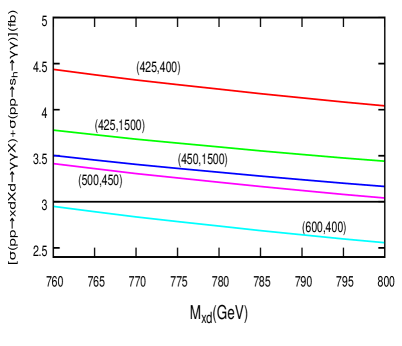
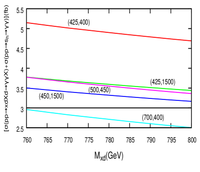
Figure 8: The combined contribution to the inclusive diphoton production cross section from $xd$ pair production channel and $s_{h}$ resonant production channel as a function of $M_{xd}$ with different choices of $(v_{s},M_{xl})$. The two panels represent the same configurations as in Fig.7.

IV Conclusions

In this work we have considered an $E_{6}$ motivated extension of the SM where the larger symmetry groups are broken at a very high scale and a residual $U(1)$ gauge symmetry is the only remaining symmetry beyond the unbroken SM gauge symmetry. This additional $U(1)$ then gets broken at the TeV scale through new scalar SM singlets giving rise to a TeV scale particle spectrum with three generations of vector-like quarks and leptons and several neutral scalars. We proposed one of the singlet dominated scalar to be the observed $750$ GeV resonance and that the diphoton resonance signal indicated by the recent LHC data might also arise from the pair production of vector-like down-type quarks with mass a little bit heavier than $750$ GeV scalar. The vector-like quarks decay into the ordinary light quark and $750$ GeV SM singlet scalar. The subsequent decay of the scalar singlet produces this diphoton resonance. We also showed that there is a wide range of parameter space in the model that could accommodate the diphoton signal, either through the more popular proposals in the literatures where the scalar is produced as an $s$-channel resonance through gluon-gluon fusion via VLQ loop-mediated processes as well as the new channel mentioned above. The prediction of such a proposal in the current theoretical framework would imply an accompanying dijet signal at the same mass with similar cross section in the $2\gamma+2j$ final state in addition to two dijet resonances at the same mass for a $4j$ final state with the cross sections about 100 times larger. Both the predictions would be verifiable as the luminosity accumulates in the upcoming runs of the LHC. We also proposed that the new production channel is a new search mode for vector-like quarks and would severely affect the current limits on vector-like quark mass which rely on its decay to SM gauge bosons and quarks. Thus, even if the 750 GeV diphoton signal indeed proves to be a fluctuation and does not survive the scrutiny of time and the upcoming high luminosity data at the LHC, the new signal for the VLQ, proposed in this work, could provide to be an interesting channel to search for new physics beyond the SM.