Pathwise error bounds in Multiscale variable splitting methods for spatial stochastic kinetics
Abstract.
Stochastic computational models in the form of pure jump processes occur frequently in the description of chemical reactive processes, of ion channel dynamics, and of the spread of infections in populations. For spatially extended models, the computational complexity can be rather high such that approximate multiscale models are attractive alternatives. Within this framework some variables are described stochastically, while others are approximated with a macroscopic point value.
We devise theoretical tools for analyzing the pathwise multiscale convergence of this type of variable splitting methods, aiming specifically at spatially extended models. Notably, the conditions we develop guarantee well-posedness of the approximations without requiring explicit assumptions of a priori bounded solutions. We are also able to quantify the effect of the different sources of errors, namely the multiscale error and the splitting error, respectively, by developing suitable error bounds. Computational experiments on selected problems serve to illustrate our findings.
Key words and phrases:
Hybrid mesoscopic model; Mean square bounds; Continuous-time Markov chain; Jump process; Rate equation2010 Mathematics Subject Classification:
Primary: 65C20, 60J22; Secondary: 65C40, 60J271. Introduction
Mesoscopic spatially extended stochastic models are in frequent use in many fields, with notable examples found in cell biology, neuroscience, and epidemiology. The traditional macroscopic description is a partial differential equation (PDE) governing the flow of concentration field variables in a generalized reaction-transport process. Whenever a certain concentration is small enough, discrete stochastic effects become more pronounced, thus invalidating the assumptions behind the macroscopic model. An alternative is then to turn to a mesoscopic stochastic model, a continuous-time Markov chain over a discrete state-space. This model often remains accurate at an acceptable computational complexity.
In the traditional non-spatial, or well-stirred setting, early work by Kurtz connected theses two descriptions via limit theorems, showing essentially that continuous approximations emerge in the limit of large molecular numbers, sometimes referred to as the “thermodynamic limit”. Strong approximation theorems in the same setting were later also developed (for more of this, see the monograph [14] and the references therein).
Multiscale-, or hybrid descriptions, in which the two scales are blended has since attracted many researchers. The focus of the research tend to fall into one of two categories; either “theoretical” and concerning error bounds and rate of convergence, or more “practical” by developing actual implementations and general software.
In the first category, tentative analysis of specific examples are found in [4], while [19, 17] are of more general character and based on averaging techniques, and conditional expectations, respectively. A related analysis in the sense of mean-square convergence for operator splitting techniques is found in [11]. In [18] the issue of a proper scaling is stressed and similar remarks are made in [15], where notably, a practical multiscale simulation algorithm is also devised.
Towards the more algorithmic side, an early suggestion for a hybrid method in [16] came to be followed up by several others [1, 23, 24]. Related multiscale algorithms based on quasi equilibrium assumptions are found in [9, 7], and the method in [13] relied on the macroscale description as a preconditioner to bring out parallelism.
With few exceptions [3, 25], the main body of work has been done in the well-stirred (or 0-dimensional) setting. Since the work [12] and the software described in [8], however, it is fairly well understood how spatial models are to be developed. Here the computational complexity is much higher such that multiscale methods appear as a very attractive alternative. This is the starting point for the present contribution.
The goal with the analysis of the paper is twofold. We will firstly deal with the multiscale analysis required for the splitting of the state variable into a stochastic and a deterministic part, respectively. Secondly, we will also deal with the numerical analysis relied upon when designing a basic but representative time-discretization of this approximating process.
The paper is organized as follows: below we first summarize the main results of the paper. In §2 we work through the description of mesoscopic reactive processes as continuous-time Markov chains with a focus on the spatial case. A substantial effort is made to avoid any possibly circular assumptions on the solution regularity, but rather to prove all results within a single coherent framework. The analysis of the multiscale approximation is found in §3, where error bounds for both the multiscale and the splitting errors are developed. Our approach is pathwise in the sense that the errors are measured in over a single probability space. Selected numerical examples are presented in §4, and a concluding discussion is offered in §5.
1.1. Summary of main results
A brief orientation of the technical results of the paper is as follows:
-
(1)
Theorem 2.4 proves a strong regularity result for the type of spatial reactive processes considered in the paper.
-
(2)
Theorem 2.5 proves the corresponding result in the setting of a multiscale framework. In particular, this reveals partial assumptions for when a multiscale description is meaningful.
- (3)
- (4)
- (5)
In this list, items 1–3 proves well-posedness and stability for the various involved processes. Following the celebrated Lax principle, items 4–5 next proves convergence and error estimates by an investigation of the consistency in the different approximations.
2. Mesoscopic spatial stochastic kinetics
We devote this section to some technical developments; §2.1–2.2 summarize reaction-transport type modeling over irregular lattices, and regularity results under suitable model assumptions are developed in §2.3. The variable splitting setup to be studied is similarly detailed in §2.4–2.5, where the corresponding regularity results are evaluated anew.
Throughout the paper we shall remain in the framework of continuous-time Markov processes on a discrete state-space, albeit with some special structure imposed from the spatial context. Assuming a process counting at time the number of entities in each of compartments, a set of state transitions is generally prescribed by
| (2.1) |
for . To enforce a conservative chain which remains in , we assume whenever .
2.1. Continuous-time Markov chains on irregular lattices
In the traditional well-stirred setting we have species interacting according to chemical reactions in some fixed volume . Given an initial state , the dynamics is then fully described by the stoichiometric matrix , and , the set of propensities. Assuming a probability space supporting -dimensional Poisson processes, the state is evolved according to [14, Chap. 6.2]
| (2.2) |
for species and with standard unit-rate independent Poisson processes , .
If the assumption of a spatially uniform distribution no longer holds a notation for spatial dependency needs to enter. The given continuous volume is discretized into smaller voxels and the state , where is the number of molecules of the th species in the th voxel. The assumption of global homogeneity is replaced with a local assumption about uniformity in each voxel such that the dynamics (2.2) may be used anew on a per-voxel basis. Adding suitable terms covering any specified transport process we get
| (2.3) | ||||
where is the rate per unit of time for species to move from the th voxel to the th.
An important consequence of the integral representation (2.3) is Dynkin’s formula [6, Chap. 9.2.2]. For a suitable function,
| (2.4) | ||||
expressed in terms of the stopped process for a stopping time in some suitable norm, and an arbitrary real number. In (2.4), is an all-zero column vector of suitable height and with a single 1 at position .
2.2. Mesh regularity
The subdivision of the total volume into smaller voxels is in principle arbitrary. However, any meaningful analysis will clearly depend to some extent on the regularity of this discretization.
Definition 2.1 (Mesh regularity parameters).
We consider a geometry in dimensions and total volume , discretized by any member in the set of meshes . For any such mesh consisting of voxel volumes we assume that it holds that
| (2.5) | ||||
| (2.6) | ||||
| (2.7) |
for constants , , , and average voxel volume . Hence under this parametrization we may write
Informally, (2.5) measures how far the meshes in are from being uniform, (2.6) ensures that no single voxel collapses into a voxel in less than dimensions, and (2.7) that the connectivity of the mesh is bounded. In the present paper (2.6) is not used explicitly; this assumption assures a connection to the macroscopic viewpoint in that a concentration variable may be meaningfully defined everywhere.
2.3. Solution regularity
We next ensure the well-posedness of (2.3) by deriving some pathwise bounds on this process. To get some feeling for what is going on we first look briefly at the corresponding PDE-setting.
Assume for simplicity that the transport rates have been chosen as a consistent discretization of the operator under homogeneous Neumann conditions at the mesh . Denoting a deterministic time-dependent concentration variable by for and , a macroscopic reaction-diffusion PDE corresponding to (2.3) reads
| (2.8) |
for certain nonlinear rates , to be prescribed below. Equipped with suitable initial data, (2.8) can be expected to be a well-posed initial-boundary value problem in for any .
For the stochastic case (2.3), and in the non-spatial setting, an analysis in the form of assumptions and various a priori bounds has been developed previously [10]. We borrow many ideas from this work in what follows.
The propensities in (2.3) generally obey the density dependent scaling such that for some dimensionless function [14, Chap. 11]. We further expect from a physically realistic model that the number of molecules in an isolated volume can somehow be bounded a priori. To this end we postulate the existence of a weighted norm
| (2.9) |
normalized such that . Following [10] we formulate
Assumption 2.2 (Reaction regularity).
For a mesh consisting of voxel volumes we assume the density dependent scaling,
| (2.10) | ||||
| where is independent of the mesh and further satisfies, | ||||
| (2.11) | ||||
| (2.12) | ||||
| (2.13) | ||||
With the exception of , all parameters are assumed to be non-negative.
When considering spatially varying solutions, the natural analogue to (2.9) is
| (2.14) |
for an all-unit column vector of suitable height. Our starting point is Dynkin’s formula (2.4). We find
| where | ||||
| (2.15) | ||||
We quote the following convenient inequality.
Lemma 2.1 (Lemma 4.6 in [10]).
Let with and . Then for integer we have the bounds
| (2.16) | ||||
| (2.17) |
Using Lemma 2.1 (2.16), Assumption 2.2 (2.10)–(2.12), and Definition 2.1 (2.5) we obtain, where for brevity ,
| (2.18) |
where , , and . Combining (2.15) and (2.18) and using Young’s inequality several times we may obtain a bound of the form
| (2.19) |
for some . Using Gronwall’s inequality and letting we arrive at
Theorem 2.2.
Proof.
It remains to prove that almost surely as . Suppose to the contrary that does not converge a.s. to as . Define . By the assumption and, for any , and for all ,
In other words, for every , and forms an increasing sequence with respect to . Using the Lebesgue monotone convergence theorem together with , we get that . However, is bounded from above independently of and thus we have a contradiction. ∎
Notably, when small voxels are present and quadratic reactions which are not -neutral are allowed (i.e. ), then an investigation of in (2.19) reveals that the second order moment and higher may grow fast as .
To achieve pathwise convergence results we will need a stronger regularity guarantee which requires control of the martingale part via Burkholder’s inequality. To this end we define the quadratic variation of a real-valued process by
| (2.21) |
where the partition for which and where the limit is in probability.
Lemma 2.3.
Proof.
Let and for be the successive jump times of . Then
Under the stopping time is non-explosive with probability 1 and the number of jumps is finite in . Thus we can use the inequality to get
The right-hand side can be written as a Lebesgue-Steiltjes integral,
with the counting process . Taking the expectation yields
Using Lemma 2.1 (2.17) and Assumption 2.2 (2.10) and (2.12),
Relying on the moment bound in Theorem 2.2 we let to arrive at the stated bound. ∎
We consider the following strong sense of pathwise locally bounded processes:
| (2.25) |
Theorem 2.4 (Regularity).
Proof.
This result follows as a combination of Theorem 2.2 and Lemma 2.3. We find that
with defined in (2.15). The quadratic variation of the local martingale can be estimated via Lemma 2.3,
| (2.26) |
Assume first that . Using the previously developed bound in (2.18) and (2.19) for the drift part we get
| Combining with (2.26) we find after using Burkholder’s inequality [20, Chap. IV.4], | ||||
| For clarity, writing we find that | ||||
Gronwall’s inequality now implies that is bounded in terms of the initial data and time . By Fatou’s lemma the claim follows by letting .
2.4. Scaling
We shall now regard the transport rates, the reaction rates, and the magnitude of the state variables as problem parameters which may induce a scale separation. Although a completely general multiscale analysis is possible within the current framework, to fix our ideas and in the interest of a transparent presentation, we consider a concrete, but still quite general two-scale separation.
Condition 2.3 (Scale separation).
Let a scale vector be given. The transport- and reaction rates are assumed to obey the scaling laws
| (2.27) | ||||
| (2.28) | ||||
| for , , and . For the state variables we define | ||||
| (2.29) | ||||
where is the scaling of the rate (fast/slow) while follows from the number of species involved in transition such that . Let the complete scaling be
The dynamics is considered for , with respect to . Also, all non-dimensionalized constants and propensities are understood to be with respect to .
It is possible to analyze also the general case where the species scale differently in different voxels, i.e. . However, this analysis is complicated by the fact that the results then take place in a transient regime, and, in turn, this regime is difficult to generally estimate.
We make a slight abuse of notation by employing as if it was the -by- matrix . Using a similar convention for we may write (2.28) in the compact form
| (2.30) |
To take a concrete example: the bimolecular reaction at rate obeys (2.28) with for and one of the species scaling macroscopically as . If both species are macroscopic, then instead at the same scaling of the rate .
Following Condition 2.3 we thus divide the species into two disjoint groups, and , with . Informally, we suppose that species in low copy numbers are in and species in large copy numbers are in . Under an appropriate enumeration of the species this implies the choice of scaling for and for in (2.29). Following this ordering we also write and , where and for .
We find from (2.3) the governing equation
| (2.31) | ||||
For the existence of scale separation it is critical to find conditions such that according to some weight-vector , for remains whenever is , assuming that and both are with respect to . Unfortunately, the assumptions and analysis in §2.3 all concerned the unscaled variable , which is now assumed to be . In fact, it is not difficult to see that with, say, replacing throughout Assumption 2.2, and requiring that all constants be independent of , the results in §2.3 are straightforwardly translated into bounds in terms of the -norm of . Since this is just the -norm of itself, however, it scales as . What is additionally required is that the weight-vector can be selected independently of .
Assumption 2.4 (Reaction regularity, scaled case).
The previous assumption of density dependent propensities (2.10) is assumed to hold. We further assume the existence of a vector , independent of , such that
| (2.32) | ||||
| (2.33) | ||||
| (2.34) |
All parameters are assumed to be independent of and non-negative (with negative values allowed for ).
Equipped with this assumption we revisit the regularity results of §2.3. To this end we consider a version of scaled with ,
| (2.37) | ||||
| where the scaled state space is just | ||||
| (2.38) | ||||
and .
Theorem 2.5 (Regularity, scaled case).
Under Condition 2.3, Theorem 2.2 and 2.4 both hold with the new Assumption 2.4 replacing the previous Assumption 2.2 and with replacing . In particular:
-
(1)
The constant in Theorem 2.2 can be selected independently of .
-
(2)
If either and is with respect to , or and is , then so is for , with respect to .
2.5. Multiscale splittings
We shall consider two multiscale splittings: one “exact” in continuous time and one “numerical” in discrete time-steps of length .
Thus we firstly define , for in and using that ,
| (2.39) | ||||
| while for in , and the Poisson process is approximated by a deterministic process, | ||||
| (2.40) | ||||
In general, there is no guarantee that remains positive even when is a conservative chain. For example, the presence of a dimerization reaction, say, at rate can reach negative values of when is approximated by a continuous variable. In this example one can avoid this problem by reinterpreting the rate as . In what follows we will for simplicity assume that all models are conservative and remain in the non-negative orthant, presumably after employing some kind of limiters on the rates.
To see how a result similar to Theorem 2.5 might be obtained for the new process , we start anew from Dynkin’s formula, appropriately modified for the semi-continuous setting. We find
| (2.41) | ||||
| where | ||||
| (2.42) | ||||
and where for brevity (compare (2.15)). Using Lemma 2.1 (2.16) we find
| (2.43) |
where and are defined below (2.18). The goal here is to obtain a bound (compare (2.18)–(2.19)) and it is not difficult to see what assumption is required.
Assumption 2.5 (Reaction regularity, semi-continuous case).
This assumption can be understood as firstly, a signed bound (2.32) on the drift-part for the fully coupled system, and secondly, the extra assumption due to stochasticity (2.44), which here applies only to , that is, to the stochastic part.
Using this in (2.43) we find (compare (2.18))
| (2.45) |
and following the steps in the proofs of Theorems 2.4 and 2.5 we obtain after some work the following result.
Theorem 2.6 (Regularity, semi-continuous case).
The statement of Theorem 2.5 applies also to the approximating process with Assumption 2.5 taking the role of Assumption 2.4. The existence of solutions then concerns the semi-continuous space and we note that the remark following Theorem 2.5 concerning the dependence on the mesh regularity remains valid since is present in (2.45).
In practice, a numerical method is required to simulate . The most straightforward way is to evolve the stochastic and deterministic parts in different steps, introducing a new process which approximates . Following the partition of unity idea in [11] we define the kernel step function
| (2.46) |
Then for in ,
| (2.47) | ||||
| and for in , | ||||
| (2.48) | ||||
For regularity we start anew from the semi-continuous Dynkin’s formula,
| (2.49) | ||||
| where this time | ||||
| (2.50) | ||||
and where as before . This leads us to
Assumption 2.6 (Reaction regularity, split-step case).
In other words, (2.51) bounds the drift of the stochastic and continuous parts individually, while as before (2.44) is employed to bound the quadratic variation of the stochastic part alone.
Following again the steps in the previous proofs we obtain
Theorem 2.7 (Regularity, split-step case).
The approximation gives rise to a multiscale error, whereas induces a splitting error. Quite generally, any practical numerical method relies on this very structure in . Insight into the nature of the total error thus follows from a consistent analysis of both approximations. This is the purpose with the next section.
3. Error analysis
We present in this section the error analysis of the two approximations (2.39)–(2.40) and, respectively, (2.47)–(2.48). Theorems 2.5, 2.6, and 2.7 assert that all processes are uniformly stable in finite time. By the Lax principle the task has therefore been reduced to an investigation of the degree of consistency of the two approximations. Preliminary lemmas for this are discussed in §3.1, followed by the actual error analysis in §3.2–3.3. In order not to lose the oversight, some material heavily relied upon are developed separately in Appendix A and B.
3.1. Preliminary estimates
Intuitively, the same version of a Poisson process evaluated at two different operational times should enjoy a bounded difference, provided of course the times themselves are bounded in some suitable sense. A precise formulation of this property is related to Doob’s optional sampling theorem [20, Theorem 17, Chap. I.2] and has only just recently been investigated [15, 2] for the -norm, and in [11] for the -norm.
Lemma 3.1.
Let be a unit-rate -adapted Poisson process, and let be a bounded stopping time. Then
| (3.1) | ||||
| (3.2) |
Proof.
Lemma 3.2.
Let be a unit-rate -adapted Poisson process, and let , be bounded stopping times. Then
| (3.3) | ||||
| (3.4) | ||||
Proof.
Remark.
We will use Lemma 3.2 in the following form. Assuming has been bounded a priori by some value we get by combining (3.3) with (3.4) that
| (3.5) |
Let be the filtration adapted to . Then for a fixed , is a stopping time [2, Lemma 3.1] with respect to
Intuitively, as , the event depends on during and on all other processes during . However, as , are independent, is still a martingale with respect to (and not only with respect to ). Hence we can apply the stopping time theorems to and the previous lemmas therefore apply. The result stays true for the approximating process (and later ). Hence, given the bound
| (3.6) |
we get from (3.5) that
| (3.7) |
3.2. Multiscale convergence
This section develops a bound for the multiscale error made in the approximation . Throughout §2, a certain weighted norm which greatly simplified the theory was used. However, in the present case of bounding errors we are interested in the more conventional -norm,
| (3.8) |
where, for convenience, from now on we shall write instead of .
Let and define the joint stopping time
| (3.9) |
Recall the stopping time from the remark after Lemma 3.2. Clearly, for any fixed , is still a stopping time.
The first step in the analysis is to split the error in one part which is bounded and one part which is not,
| (3.10) |
The requirement to be able to control the contribution from the non-bounded part motivates the following lemma:
Lemma 3.3.
For any , there exists a constant independent from and such that
| (3.11) | ||||
| (3.12) | ||||
| (3.13) |
Proof.
Theorem 2.5 yields
Since and are equivalent bounds we have an a priori bound
with independent from . By Cauchy-Schwartz’s inequality,
Using that
we find from Markov’s inequality the bound
Using the second part of Theorem 2.5 and the equivalence of norms, it is possible to bound the first term on the right independently from and . Reasoning similarly for the terms depending on and we get the stated result. ∎
To formulate the main result of this section we let
| (3.14) |
and the analogous definition for . In words, contains the reactions which affect any species . We additionally define the two effective exponents
| (3.15) | ||||
| (3.16) |
Note that, if the transport rates do not scale with , we generally get and .
Theorem 3.4 (Multiscale error, bounded version).
Proof.
First notice that, since the processes are uniformly bounded with respect to , so is . Thus according to Lemma A.1,
with
Similarly, according to Lemma A.2,
where
| (3.18) |
Thus using the Gronwall inequality we find firstly,
| Using this and Gronwall’s inequality a second time gives | ||||
Suppose for the moment that is uniformly bounded by with respect to and . As the processes are bounded by , and we get the stated result.
The extra assumption that is uniformly bounded can easily be removed by changing the definition of in (3.9) into
∎
The two terms in the error bound can be interpreted as firstly, the error introduced in the macro-species, , and secondly, the error made in the meso-species, , respectively.
In order to obtain a theorem also in the unbounded case, the growth of the local Lipschitz constants has to be controlled, and so we make the following convenient assumption:
Assumption 3.1.
There exists such that . Furthermore, we assume for each such that that . Hence the Lipschitz constants associated with these transitions are bounded independently from .
As in the appendix we use the notation “” to indicate that for some constant which is with respect to , , and .
Theorem 3.5 (Multiscale error).
Proof.
The proof here concerns the case . The special case from Assumption 3.1 where and for some (and thus ) is similar but requires some cumbersome notation and is therefore omitted. Select for some and let , . Following the same pattern as in the proof of Theorem 3.4 we get
Thus using Lemma 3.3,
As can be made arbitrarily large while and can be made arbitrarily close to (i.e. and ), we arrive at the stated bound. ∎
Remark.
It is possible to get a convergence result for the case . However, in this case the error bound is of the form and the dominating part can be traced back to Lemma 3.3.
3.3. Splitting convergence
We next consider the error in the approximation , that is, the splitting error. For this part we are able to prove a somewhat weak error bound in the general case, while the situation improves considerably if the processes are assumed to be bounded a priori.
Theorem 3.6 (Splitting error, bounded version).
Proof.
As before one can appreciate the two terms of the error as the error made in the meso-species, , and , the error introduced in the macro-species.
Theorem 3.7 (Splitting error).
Proof.
Following the same pattern as in the proof of the bounded version, it is easy to show that for each ,
We conclude the argument using Lemma 3.3, which implies that
uniformly with respect to . ∎
4. Numerical examples
We now proceed to illustrate our main findings through some prototypical cases. An all-linear isomerization-type system is investigated in §4.1 and a nonlinear catalytic model in §4.2.
In the experiments below we considered reactions taking place in a one-dimensional geometry under periodic boundary conditions. The geometry was discretized into 10 equally spaced segments and a diffusion process implemented via the standard 2nd order finite difference stencil, re-interpreted as linearly dependent transition rates. As for the initial data, we let each segment contain either 10 or 20 molecules for the mesoscopic (discrete) species and or for the macroscopic (continuous) species, respectively.
The exact dynamics (2.31) was simulated in an operational time framework. Here we relied on an implementation of the All Events Method [5], essentially a spatial extension of the Common Reaction Path Method [21] which evolves (2.31) using separate Poisson processes for all events.
The multiscale approximation (2.39)–(2.40) falls under the scope of Piecewise Deterministic Markov Processes (PDMPs) for which accurate methods have been proposed [22]. We implemented this through the use of event-detection in solvers for Ordinary Differential Equations (ODEs). Notably, this allows for a fully consistent coupling with (2.31) in operational time.
Finally, the split-step approximation (2.47)–(2.48) was implemented. This is quite straightforward via the kernel step function representation and executes very efficiently. The split-step error is much more challenging to determine accurately than the multiscale error is. In fact, on a predetermined grid in time the split-step approximation in (2.47) was often found to be exactly equal to the multiscale approximation in (2.39), thus requiring many realizations for even a very crude estimate.
We make repeated use of the estimator
| (4.1) | ||||
| for independent trajectories . A basic confidence interval is obtained by computing | ||||
| (4.2) | ||||
such that the error in the estimator (4.1) is .
4.1. Isomerization
We first consider the simple linear isomerization reaction pair,
| (4.3) |
In order for this example to develop a scale separation, for , the diffusion rate is set to in either direction and per molecule, and for to . By selecting and , a scale separation occurs, with and . We may thus evolve the system by the multiscale approximation (2.39)–(2.40), letting remain discrete while is approximated with a continuous scaled variable.
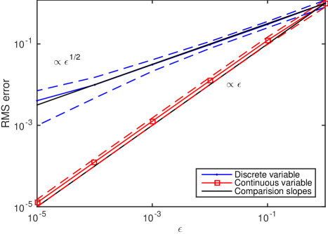
Although the unscaled system is closed, from the perspective of scale separation the system scales unfavorably with and hence falls under the scope of Theorem 3.5. We have and in (3.15)–(3.16) and thus expect a mean square error behaving like for the macroscopic species and for the mesoscopic species. This is verified in Figure 4.1 where the multiscale error for the two components is examined.
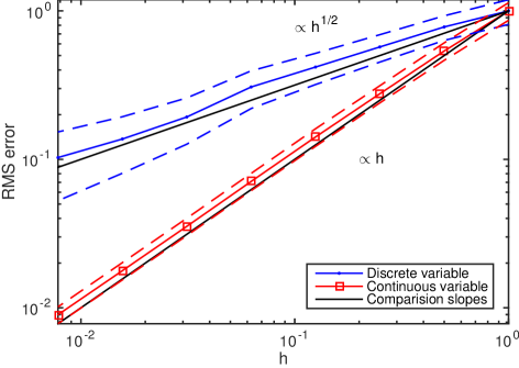
Since Theorem 3.6 is formally not applicable, the only result valid is the guaranteed convergence of Theorem 3.7. Nevertheless, in Figure 4.2 the split-step error for the two species have been plotted separately. The different terms of the error estimate in Theorem 3.6 are clearly visible, suggesting that the uniform bounds on the processes, as required by Theorem 3.6, may in fact be relaxed.
Convergence results similar to those of [4] and [18] are here consequences of Theorem 3.5, with the added benefit of an error estimate. Indeed, Theorem 3.5 yields that the difference between and goes to 0 and the convergence of is easy to study. Using (2.39) and (2.40) for voxel yields
| (4.4) |
since , and,
| (4.5) |
Hence for this simple system, the limit for is trivial.
4.2. Catalytic reactions
We consider the following pair of catalytic reactions:
| (4.9) |
We assume that species and are abundant and , and species and are . For the diffusion we put and , and for the rates and . The system so defined is closed since there is no coupling from the macro-species to the meso-species (take in Assumption 2.4). This property carries over to the multiscale and split-step approximations (cf. Assumptions 2.5 and 2.6).
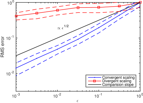
For the scale separation, we get the critical exponents and Theorem 3.4 predicts a slow convergence of in the RMS sense. However, since the meso-species do not depend on the macro-species the corresponding error is in fact . According to the discussion following the proof of Theorem 3.4, the RMS is therefore and is observed in the macroscopic species only. By the same argument, and from the remark following the proof of Theorem 3.6, we predict that the RMS of the split-step error is .
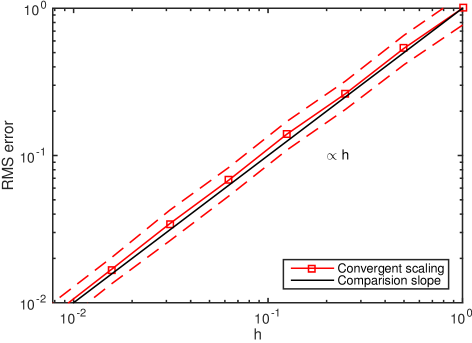
Experimental results verifying this are shown in Figure 4.3 for the multiscale error (“convergent scaling”) and in Figure 4.4 for the split-step error.
Like in the previous example, convergence results similar to those of [4] and [18] are consequences of Theorem 3.4. This time, (2.39) and (2.40) are almost independent of ; only the diffusion for and depend on and, since , it vanishes in the limit. For voxel ,
| (4.10) | ||||
| (4.11) |
The defining equations for and are similar. Thus the limit in this case is not a trivial process, stressing that non-trivial models can be described within the framework.
4.3. Catalytic reactions: case of unclear scale separation
It is interesting to turn the scales of the catalytic model around. If we instead let species and be , while and are , the topology does not change and we still have a closed system. We put , , and use the slow diffusion . The critical exponents become and and thus none of the results apply. Although Figure 4.3 (“divergent scaling”) does not strictly exclude the possibility of convergence, the error certainly does not go down convincingly.
5. Conclusions
In this paper we have developed a coherent framework for analyzing certain multiscale methods for continuous-time Markov chains of a general spatial structure. Concrete assumptions and conditions have been discovered that enables a multiscale description and a consistent formulation of the approximating methods in operational time. Notably, through explicit a priori results, all processes are well-posed and the framework does not rely on any heuristic prior bounds.
The analysis distinguishes between two separate sources of errors, namely the multiscale error and the split-step error. The first is due to an approximate stochastic/deterministic variable splitting strategy, a kind of stochastic homogenization technique. The second emerges when this approximating process in turn is evolved in discrete time-steps. Notably, we found theoretically how the split-step error is composed of factors remindful of the terms making up the multiscale error, thus connecting the two in a qualitative sense. The behavior of these errors were also examined experimentally via actual implementations of the methods. Although some of the boundary cases are difficult to handle theoretically, in particular when confronted with open systems, the numerical experiments support the sharpness of our theoretical predictions.
The work opens up for some interesting possibilities. Clearly, an ideal implementation should allow the split-step error to be about as large as the multiscale error. The fully discrete approximation is amenable to several efficient algorithms developed for numerical methods for partial differential equations, including for example multigrid techniques. An interesting challenge to which we would like to return is to develop practical procedures for computing accurate error estimates. We believe this is doable following the theory laid out in the paper.
Acknowledgment
Many detailed suggestions by the two referees have helped us to clarify and improve the paper.
The work was supported by ENS Cachan (A. Chevallier) and by the Swedish Research Council within the UPMARC Linnaeus center of Excellence (S. Engblom).
Appendix A The multiscale error
Below are the statements and proofs of the two critical lemmas used in the proof of Theorem 3.5. Recall the definition of the two effective exponents and in (3.15)–(3.16).
Lemma A.1.
To improve the readability of the proof, we use the notation “” to indicate that for some constant which is with respect to , , and . When the processes are assumed to be bounded a priori, clearly, , for any constant . In the unbounded case, Assumption 3.1 yields similarly for any constant . We additionally let be the constants in the norm equivalence
| (A.2) |
Proof.
We focus first on a single voxel and analyze the errors on species from and , respectively. For , from (2.31) and (2.39),
where we have suppressed the local time arguments of the Poisson processes, available in (2.31) and (2.39).
By Jensen’s inequality and the bound on the mesh connectivity in Definition 2.1 (2.7) we get
where in terms of
First we need to bound the -norm:
Then using the Lipschitz bound (2.34) in Assumption 2.4:
Thus,
Using the same method for , we conclude
Hence using Lemma 3.2 (Remark) and again the Lipschitz bound we get
Relying on the same arguments we readily find
and the identical bound for .
For , we similarly get
where
The analysis is now slightly different. Species from the second group have a large number of molecules, so is expected to remain close to its mean value. We thus introduce the centered Poisson processes ,
Using that the quadratic variation of is and the martingale stopping time theorem we get
Using Cauchy-Schwartz for the remaining integral part and following the same approach for and we get
as well as an identical bound for .
We thus get for the th voxel,
| (A.3) |
Summing over we get the stated result with , , and . ∎
Lemma A.2.
Proof.
For voxel and for ,
We keep the same notation as in the previous lemma and thus write
| where | ||||
In the same spirit we find
and an identical bound for .
Continuing with ,
where
Using the same techniques developed previously we find
In much the same spirit we get
along with an identical bound for .
Combined we thus get for the th voxel,
| (A.5) |
Summing over we get the stated result. ∎
Appendix B The split-step error
The consistency of the numerical split-step method hinges on the regularity of the kernel function . The following lemma (borrowed from [11, Lemma 3.7]) paired with the strong regularity of the involved processes provides for the order estimate in Theorems 3.6 and 3.7. Note that the result can be thought of as càdlàg-version of the Riemann-Lebesgue lemma.
Lemma B.1.
([11, Lemma 3.7]) Let be a globally Lipschitz continuous function with Lipschitz constant and let be a piecewise constant càdlàg function. Then
| (B.1) |
where the total absolute variation may be exchanged with the square root of the quadratic variation . If is a multiple of , then the first term on the right side of (B.1) vanishes.
The proofs of the following two lemmas follow closely the ideas in the proofs of Lemmas A.1 and A.2, but using in addition Lemma B.1 and Theorem 2.7 to bound certain additional terms.
Lemma B.2.
Lemma B.3.
References
- Alfonsi et al. [2005] A. Alfonsi, E. Cancés, G. Turinici, B. D. Ventura, and W. Huisinga. Adaptive simulation of hybrid stochastic and deterministic models for biochemical systems. ESAIM: Proc., 14:1–13, 2005. doi:10.1051/proc:2005001.
- Anderson et al. [2011] D. F. Anderson, A. Ganguly, and T. G. Kurtz. Error analysis of tau-leap simulation methods. Ann. Appl. Probab., 21(6):2226–2262, 2011. doi:10.1214/10-AAP756.
- Arampatzis et al. [2014] G. Arampatzis, M. Katsoulakis, and P. Plecháč. Parallelization, processor communication and error analysis in lattice kinetic monte carlo. SIAM J. Numer. Anal., 52(3):1156–1182, 2014. doi:10.1137/120889459.
- Ball et al. [2006] K. Ball, T. G. Kurtz, L. Popovic, and G. Rempala. Asymptotic analysis of multiscale approximations to reaction networks. Ann. Appl. Probab., 16(4):1925–1961, 2006. doi:10.1214/105051606000000420.
- Bauer and Engblom [2015] P. Bauer and S. Engblom. Sensitivity estimation and inverse problems in spatial stochastic models of chemical kinetics. In A. Abdulle, S. Deparis, D. Kressner, F. Nobile, and M. Picasso, editors, Numerical Mathematics and Advanced Applications: ENUMATH 2013, volume 103 of Lecture Notes in Computational Science and Engineering, pages 519–527, Berlin, 2015. Springer. doi:10.1007/978-3-319-10705-9_51.
- Brémaud [1999] P. Brémaud. Markov Chains: Gibbs Fields, Monte Carlo Simulation, and Queues. Number 31 in Texts in Applied Mathematics. Springer, New York, 1999.
- Cao et al. [2005] Y. Cao, D. T. Gillespie, and L. R. Petzold. The slow-scale stochastic simulation algorithm. J. Chem. Phys., 122(1):014116, 2005. doi:10.1063/1.1824902.
- Drawert et al. [2012] B. Drawert, S. Engblom, and A. Hellander. URDME: a modular framework for stochastic simulation of reaction-transport processes in complex geometries. BMC Syst. Biol., 6(76):1–17, 2012. doi:10.1186/1752-0509-6-76.
- E et al. [2005] W. E, D. Liu, and E. Vanden-Eijnden. Nested stochastic simulation algorithm for chemical kinetic systems with disparate rates. J. Chem. Phys., 123(19):194107, 2005. doi:10.1063/1.2109987.
- Engblom [2014] S. Engblom. On the stability of stochastic jump kinetics. Appl. Math., 5(19):3217–3239, 2014. doi:10.4236/am.2014.519300.
- Engblom [2015] S. Engblom. Strong convergence for split-step methods in stochastic jump kinetics. SIAM J. Numer. Anal., 53(6):2655–2676, 2015. doi:10.1137/141000841.
- S. Engblom, L. Ferm, A. Hellander, and P. Lötstedt [2009] S. Engblom, L. Ferm, A. Hellander, and P. Lötstedt. Simulation of stochastic reaction-diffusion processes on unstructured meshes. SIAM J. Sci. Comput., 31(3):1774–1797, 2009. doi:10.1137/080721388.
- S. Engblom [2009] S. Engblom. Parallel in time simulation of multiscale stochastic chemical kinetics. Multiscale Model. Simul., 8(1):46–68, 2009. doi:10.1137/080733723.
- Ethier and Kurtz [1986] S. N. Ethier and T. G. Kurtz. Markov Processes: Characterization and Convergence. Wiley series in Probability and Mathematical Statistics. John Wiley & Sons, New York, 1986.
- Ganguly et al. [2015] A. Ganguly, D. Altıntan, and H. Koeppl. Jump-diffusion approximation of stochastic reaction dynamics: Error bounds and algorithms. Multiscale Model. Simul., 13(4):1390–1419, 2015. doi:10.1137/140983471.
- Haseltine and Rawlings [2002] E. L. Haseltine and J. B. Rawlings. Approximate simulation of coupled fast and slow reactions for stochastic chemical kinetics. J. Chem. Phys., 117(15):6959–6969, 2002. doi:10.1063/1.1505860.
- Jahnke and Kreim [2012] T. Jahnke and M. Kreim. Error bound for piecewise deterministic processes modeling stochastic reaction systems. Multiscale Model. Simul., 10(4):1119–1147, 2012. doi:10.1137/120871894.
- Kang and Kurtz [2013] H.-W. Kang and T. G. Kurtz. Separation of time-scales and model reduction for stochastic reaction networks. Ann. Appl. Probab., 23(2):529–583, 2013. doi:10.1214/12-AAP841.
- Plyasunov and Arkin [2006] S. Plyasunov and A. P. Arkin. Averaging methods for stochastic dynamics of complex reaction networks: Description of multiscale couplings. Multiscale Model. Simul., 5(2):497–513, 2006. doi:10.1137/050633822.
- Protter [2005] P. E. Protter. Stochastic Integration and Differential Equations. Number 21 in Stochastic Modelling and Applied Probability. Springer, Berlin, 2nd edition, 2005. Version 2.1.
- Rathinam et al. [2010] M. Rathinam, P. W. Sheppard, and M. Khammash. Efficient computation of parameter sensitivities of discrete stochastic chemical reaction networks. J. Chem. Phys., 132(3):034103, 2010. doi:10.1063/1.3280166.
- Riedler [2013] M. G. Riedler. Almost sure convergence of numerical approximations for piecewise deterministic Markov processes. J. Comput. Appl. Math., 239(0):50–71, 2013. doi:10.1016/j.cam.2012.09.021.
- Salis et al. [2006] H. Salis, V. Sotiropoulos, and Y. N. Kaznessis. Multiscale Hy3S: Hybrid stochastic simulation for supercomputers. BMC Bioinformatics, 7(93), 2006. doi:10.1186/1471-2105-7-93.
- Samant et al. [2007] A. Samant, B. A. Ogunnaike, and D. G. Vlachos. A hybrid multiscale Monte Carlo algorithm (HyMSMC) to cope with disparity in time scales and species populations in intracellular networks. BMC Bioinformatics, 8(1):175, 2007. doi:10.1186/1471-2105-8-175.
- Yates and Flegg [2015] C. A. Yates and M. B. Flegg. The pseudo-compartment method for coupling partial differential equation and compartment-based models of diffusion. J. R. Soc. Interface, 12(106), 2015. doi:10.1098/rsif.2015.0141.