Corrugation of relativistic magnetized shock waves

Abstract

As a shock front interacts with turbulence, it develops corrugation which induces outgoing wave modes in the downstream plasma. For a fast shock wave, the incoming wave modes can either be fast magnetosonic waves originating from downstream, outrunning the shock, or eigenmodes of the upstream plasma drifting through the shock. Using linear perturbation theory in relativistic MHD, this paper provides a general analysis of the corrugation of relativistic magnetized fast shock waves resulting from their interaction with small amplitude disturbances. Transfer functions characterizing the linear response for each of the outgoing modes are calculated as a function of the magnetization of the upstream medium and as a function of the nature of the incoming wave. Interestingly, if the latter is an eigenmode of the upstream plasma, we find that there exists a resonance at which the (linear) response of the shock becomes large or even diverges. This result may have profound consequences on the phenomenology of astrophysical relativistic magnetized shock waves.

1 Introduction

The physics of relativistic shock waves, in which the unshocked plasma enters the shock front with a relative relativistic velocity $v_{\rm sh}\,\sim\,c$, is a topic which has received increased attention since the discovery of various astrophysical sources endowed with relativistic outflows, such as radio-galaxies, micro-quasars, pulsar wind nebulae or gamma-ray bursts. In those objects, the relativistic shock waves are believed to play a crucial role in the dissipation of plasma bulk energy into non-thermal particle energy, which is then channeled into non-thermal electromagnetic radiation (or possibly, high energy neutrinos and cosmic rays). The various manifestations of these high energy sources have been a key motivation to understand the physics of collisionless shock waves and of the ensuing particle acceleration processes (e.g. Bykov & Treumann, 2011; Bykov et al., 2012; Sironi et al., 2015) for reviews. The nature of the turbulence excited in the vicinity of these collisionless shocks remains a nagging open question, which is however central to all the above topics, since it directly governs the physics of acceleration and, possibly, radiation.

The physics of shock waves in the collisionless regime has itself been a long-standing problem in plasma physics, going back to the pioneering studies of  Moiseev & Sagdeev (1963), with intense renewed interest related to the possibility of reproducing such shocks in laboratory astrophysics (e.g. Kuramitsu et al., 2011; Drake & Gregori, 2012; Park et al., 2012; Huntington et al., 2015; Park et al., 2015). The generation of relativistic collisionless shock waves is also already envisaged with future generations of lasers (e.g. Chen et al., 2015; Lobet et al., 2015).

One topic of general interest, with direct application to the above fields, is the stability of shock waves. The study of the corrugation instability of a shock wave goes back to the early works of  D’Iakov (1958) and Kontorovich (1958), see also  Bykov (1982), Landau & Lifshitz (1987) or more recently  Bates & Montgomery (2000). General theorems assuming polytropic equations of state ensure the stability of shock waves against corrugation, in the relativistic (Anile & Russo, 1986) and/or magnetized regime (Gardner & Kruskal, 1964; Lessen & Deshpande, 1967; McKenzie & Westphal, 1970), although instability may exist in other regimes (e.g. Tsintsadze et al., 1997). In any case, the stability against corrugation does not preclude the possibility of spontaneous emission of waves by the shock front, as discussed in the above references.

The interaction of the shock front with disturbances thus represents a topic of prime interest, as it may lead to the corrugation of the shock front and to the generation of turbulence behind the shock, with possibly large amplification. The transmission of upstream Alfvén waves through a sub-relativistic shock front has been addressed, in particular, by Achterberg & Blandford (1986); more recently,  Lyutikov et al. (2012) has reported on numerical MHD simulations of the interaction of a fast magnetosonic wave impinging on the downstream side of a relativistic shock front.

The present paper proposes a general investigation of the corrugation of relativistic magnetized collisionless shock waves induced by either upstream or downstream small amplitude perturbations. This study is carried out analytically for a planar shock front in linearized relativistic MHD. This problem is addressed as follows. Section 2 provides some notations as well as the shock crossing conditions to the first order in perturbations, which relate the amplitude of shock corrugation to the amplitude of incoming and outgoing MHD perturbations of the flow. Section 3 is devoted to the interaction of a fast magnetosonic wave originating from downstream and to its scattering off the shock front, with resulting outgoing waves and shock corrugation. Section 4 discusses the transmission of upstream entropy and Alfvén perturbations into downstream turbulence. It reveals, in particular, that there exist resonant wavenumbers of the turbulence for which the amplification of the incoming wave, and consequently the amplitude of the shock crossing, becomes formally infinite. This resonant excitation of the shock front by incoming upstream turbulence may have profound implications for our understanding of astrophysical shock waves and the associated acceleration processes.

2 General considerations

We assume here a configuration in the rest frame of the downstream (shocked) plasma in which the magnetic field is exactly perpendicular to the shock normal, and in which the upstream is inflowing into the shock along the shock normal. The former assumption is a very good approximation at relativistic shock waves (Begelman & Kirk, 1990) because of Lorentz boost effects, which enhance the in-plane components of the magnetic field by the relative Lorentz factor between the upstream and the downstream plasma, notwithstanding the further compression resulting from the jump at the shock. The latter is an assumption which allows to keep the problem tractable; shock crossing at an oblique shock can be obtained analytically but at the price of an implicit equation (Majorana & Anile, 1987; Kirk & Duffy, 1999), which renders a further perturbative treatment quite complex.

2.1 Steady planar normal shock

Although the equations of shock crossing and their solutions are known for a steady planar normal shock, it is useful to recall them in order to specify the present notations. At a shock surface defined by its normal four-vector $\ell_{\mu}$, these shock crossing conditions are expressed as:

$$\left[nu^{\mu}\,\ell_{\mu}\right] \,=\, 0,$$

$$\left[T^{\mu\nu}\,\ell_{\mu}\right] \,=\, 0,$$

$$\left[{}^{\star}F^{\mu\nu}\,\ell_{\mu}\right] \,=\, 0,$$ (1)

with, in the ideal MHD description:

$$T^{\mu\nu} \,=\, \left(w+\frac{b_{\alpha}b^{\alpha}}{4\pi}\right)u^{\mu}u^{\nu}\,+\,\left(p+\frac{b_{\alpha}b^{\alpha}}{8\pi}\right)\eta^{\mu\nu}-\frac{b^{\mu}b^{\nu}}{4\pi},$$

$${}^{\star}F^{\mu\nu} \,=\, \frac{1}{2}\epsilon^{\mu\nu\alpha\beta}F_{\alpha\beta},$$ (2)

and the following definitions: $F^{\mu\nu}$ denotes the usual electromagnetic strength tensor, the metric $\eta^{\mu\nu}$ has signature $(-,+,+,+)$, $\epsilon^{\mu\nu\alpha\beta}$ denotes the Levi-Civita tensor ($+1$ for an even permutation of the indices), while $w\,\equiv\,e+p$ represents the fluid enthalpy, and $e,p,n$ respectively correspond to the fluid energy density, pressure and density; finally, $u^{\mu}\,=\,\left(\gamma,\boldsymbol{u}\right)$ represents the fluid four-velocity (we use natural units with $c=1$ everywhere in this paper) and $b^{\mu}$ the magnetic four-vector:

$$b^{\mu}\,=\,\left[u^{i}B_{i},\left(\boldsymbol{B}+u^{i}B_{i}\,\boldsymbol{u}\right)/u^{0}\right]$$ (3)

written in terms of the (apparent) magnetic field vector $\boldsymbol{B}$. Finally, in the MHD description, one has:

$${}^{\star}F^{\mu\nu}\,=\,u^{\mu}b^{\nu}-u^{\nu}b^{\mu}$$ (4)

The shock crossing conditions are then most conveniently expressed in the downstream rest frame, in which the shock surface is described by

$$\overline{\Phi}(x)\,=\,x-\overline{\beta}_{\rm f}t\,=\,0$$ (5)

with corresponding shock normal:

$$\overline{\ell}_{\mu} \,=\, \frac{\partial_{\mu}\overline{\Phi}}{\left|\partial_{\alpha}\overline{\Phi}\partial^{\alpha}\overline{\Phi}\right|^{1/2}}$$ (6)

$$\,=\, \left(-\overline{\gamma}_{\rm f}\overline{\beta}_{\rm f},\overline{\gamma}_{\rm f},0,0\right)$$

where $\overline{\gamma}_{\rm f}\,\equiv\,\left(1-\overline{\beta}_{\rm f}^{2}\right)^{-1/2}$ denotes the bulk Lorentz factor of the shock front relative to downstream.

Henceforth, downstream quantities are indexed with ₂ while upstream quantities are indexed with ₁; the notation $b_{1,2}\,\equiv\,B_{1,2}/\gamma_{1,2}$ is also used in the equations below. In the downstream frame, one has $u_{2}^{\mu}\,=\,(1,0,0,0)$ and $u_{1}^{\mu}\,=\,(\gamma_{1},\gamma_{1}\beta_{1},0,0)$. We also use the short-hand notations for the generalized enthalpy and pressure:

$$W\,\equiv\,w+\frac{b_{\alpha}b^{\alpha}}{4\pi},\quad P\,\equiv\,p+\frac{b_{\alpha}b^{\alpha}}{8\pi},$$ (7)

Figure 1 shows a sketch of the planar shock configuration, emphasizing the notions of the shock velocity ($\overline{\beta}_{\rm f}$) and of the upstream plasma ($\beta_{1}$), both expressed relative to the downstream frame.

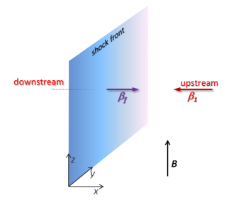
Figure 1: Sketch of the shock configuration: in the downstream plasma rest frame, the shock front moves at velocity $\overline{\beta}_{\rm f}\,>\,0$ while the upstream (unshocked) plasma is inflowing at velocity $\beta_{1}\,\simeq\,-1$. As indicated, the magnetic field carried by the inflowing upstream plasma lies along $\boldsymbol{z}$.

Given Eq. (6), the shock crossing equations (1) break down to:

$$n_{1}\gamma_{1}\left(\beta_{1}-\overline{\beta}_{\rm f}\right) \,=\, -n_{2}\overline{\beta}_{\rm f}$$ (8)

$$b_{1}\gamma_{1}\left(\beta_{1}-\overline{\beta}_{\rm f}\right) \,=\, -b_{2}\overline{\beta}_{\rm f}$$ (9)

$$W_{1}\gamma_{1}^{2}\left(\beta_{1}-\overline{\beta}_{\rm f}\right)+\overline{\beta}_{\rm f}P_{1} \,=\, -\overline{\beta}_{\rm f}\left(W_{2}-P_{2}\right)$$ (10)

$$W_{1}\gamma_{1}^{2}\beta_{1}\left(\beta_{1}-\overline{\beta}_{\rm f}\right)+P_{1} \,=\, P_{2}$$ (11)

These equations are easily solved in the strong shock ($P_{1}\,\ll\,P_{2}$) and relativistic limit ($\gamma_{1}\,\gg\,1$). Defining the magnetization parameter:

$$\sigma_{1}\,\equiv\,\frac{b_{1}^{2}}{4\pi w_{1}},$$ (12)

so that $W_{1}\,=\,b_{1}^{2}\left(1+\sigma_{1}^{-1}\right)$, assuming a cold incoming plasma $w_{1}\,=\,n_{1}m$, one finds

$$\overline{\beta}_{\rm f}\,\simeq\,\frac{2\sigma_{1}+1+\left[1+16\sigma_{1}\left(1+\sigma_{1}\right)\right]^{1/2}}{6(1+\sigma_{1})}$$ (13)

up to corrections of order $1/\gamma_{1}^{2}$. This solution matches the standard result of Kennel & Coroniti (1984), although it is given here in a simpler form. It can be approximated as:

$$\overline{\beta}_{\rm f}\,\simeq\,\begin{cases}\displaystyle{\frac{1}{3}+\frac{4\sigma_{1}}{3}}&\left(\sigma_{1}\,\ll\,1\right)\\ &\\ \displaystyle{1-\frac{1}{2\sigma_{1}}}&\left(\sigma_{1}\,\gg\,1\right)\end{cases}$$ (14)

Once $\overline{\beta}_{\rm f}$ is known, the shock crossing conditions immediately give $n_{2}$ and $b_{2}$ as a function of $n_{1}$ and $b_{1}$ respectively. One also derives

$$\frac{b_{2}^{2}}{4\pi w_{1}} \,\simeq\, \frac{1}{\overline{\beta}_{\rm f}}\left(1+\sigma_{1}\right)\gamma_{1}^{2}\left(\beta_{1}-\overline{\beta}_{\rm f}\right)\left(3\beta_{1}\overline{\beta}_{\rm f}+1\right),$$ (15)

$$\frac{w_{2}}{w_{1}} \,\simeq\, -\frac{2}{\overline{\beta}_{\rm f}}\left(1+\sigma_{1}\right)\gamma_{1}^{2}\left(\beta_{1}-\overline{\beta}_{\rm f}\right)\left(\beta_{1}\overline{\beta}_{\rm f}+1\right)$$ (16)

so that, for instance,

$$\sigma_{2}\,=\,\frac{b_{2}^{2}}{4\pi w_{2}}\,\simeq\,\begin{cases}3\sigma_{1}&(\sigma_{1}\,\ll\,1)\\ 2\sigma_{1}&(\sigma_{1}\,\gg\,1)\end{cases}$$ (17)

2.2 Shock corrugation

We now consider the influence of perturbations in the background flow on the shock. As the perturbations impinge on the shock, they induce a deformation of the shock surface, which can be written up to first order in the perturbations as:

$$\Phi(x) \,=\, \overline{\Phi}(x,t)+\delta\Phi\left(\boldsymbol{x_{\perp}},t\right)$$ (18)

$$\,=\, x-\overline{\beta}_{\rm f}t-\delta X\left(\boldsymbol{x_{\perp}},t\right)$$

with $\boldsymbol{x_{\perp}}\,\equiv\,(y,z)$. Corrrespondingly, the normal of the perturbed shock surface is written to first order in the perturbations as:

$$\ell_{\mu}\,=\,\overline{\ell}_{\mu}+\delta\ell_{\mu}$$ (19)

with

$$\delta\ell_{\mu}\,=\,-\frac{\partial_{\mu}\delta X}{\left|\partial_{\alpha}\overline{\Phi}\partial^{\alpha}\overline{\Phi}\right|^{1/2}}+\frac{\partial_{\mu}\overline{\Phi}\,\partial_{\beta}\delta X\partial^{\beta}\overline{\Phi}}{\left|\partial_{\alpha}\overline{\Phi}\partial^{\alpha}\overline{\Phi}\right|^{3/2}}$$ (20)

For the purpose of this Section, consider a harmonic perturbation on a single scale $\boldsymbol{k_{\perp}}$:

$$\delta X\left(\boldsymbol{x_{\perp}},t\right)\,=\,\delta X_{\boldsymbol{k_{\perp}}}(t)\,\,e^{i\boldsymbol{k_{\perp}}\cdot\boldsymbol{x_{\perp}}}$$ (21)

with a similar decomposition for all other variables. One then obtains:

$$\delta\ell_{\boldsymbol{k_{\perp}},\mu} \,=\, \biggl{(}-\overline{\gamma}_{\rm f}^{3}\,\delta V_{\boldsymbol{k_{\perp}}},\,\,\overline{\gamma}_{\rm f}^{3}\overline{\beta}_{\rm f}\,\delta V_{\boldsymbol{k_{\perp}}},\,\,-ik_{y}\,\overline{\gamma}_{\rm f}\delta X_{\boldsymbol{k_{\perp}}},$$ (22)

$$\quad\quad-ik_{z}\,\overline{\gamma}_{\rm f}\delta X_{\boldsymbol{k_{\perp}}}\biggr{)}$$

with

$$\delta V_{\boldsymbol{k_{\perp}}}\,\equiv\,\frac{{\rm d}}{{\rm d}t}\delta X_{\boldsymbol{k_{\perp}}}$$ (23)

The deformation of the shock surface then implies the existence of fluctuations of the various quantities of the downstream plasma at the shock. These quantities are formally obtained by the solution to the shock crossing conditions at the first order in the perturbations:

$$\left[\ell_{\mu}\,\delta\left(nu^{\mu}\right)+\delta\ell_{\mu}nu^{\mu}\right] \,=\, 0$$ (24)

$$\left[\ell_{\mu}\delta T^{\mu\nu}+\delta\ell_{\mu}T^{\mu\nu}\right] \,=\, 0$$ (25)

$$\left[\ell_{\mu}\,\delta^{\star}F^{\mu\nu}+\delta\ell_{\mu}\,^{\star}F^{\mu\nu}\right] \,=\, 0$$ (26)

For harmonic perturbations on the shock front plane in transverse Fourier space, the above equations can be written as follows:

$$n_{2}\delta\beta_{2x,\boldsymbol{k_{\perp}}}-\overline{\beta}_{\rm f}\delta n_{2,\boldsymbol{k_{\perp}}}+\overline{\gamma}_{\rm f}^{2}\left[\gamma_{1}n_{1}\left(1-\beta_{1}\overline{\beta}_{\rm f}\right)-n_{2}\right]\delta V_{\boldsymbol{k_{\perp}}} \,=\, R_{1}$$

$$-\overline{\beta}_{\rm f}\delta n_{2,\boldsymbol{k_{\perp}}}-\overline{\beta}_{\rm f}\frac{B_{2}}{4\pi}\delta B_{2z,\boldsymbol{k_{\perp}}}+\frac{\overline{\beta}_{\rm f}}{1-\hat{\gamma}_{2}}\delta p_{2,\boldsymbol{k_{\perp}}}+W_{2}\delta\beta_{2x,\boldsymbol{k_{\perp}}}+\overline{\gamma}_{\rm f}^{2}\left[\gamma_{1}^{2}W_{1}\left(1-\beta_{1}\overline{\beta}_{\rm f}\right)-W_{2}+P_{2}-P_{1}\right]\delta V_{\boldsymbol{k_{\perp}}} \,=\, R_{2}$$

$$\delta p_{2,\boldsymbol{k_{\perp}}}+\frac{B_{2}}{4\pi}\delta B_{2z,\boldsymbol{k_{\perp}}}-W_{2}\overline{\beta}_{\rm f}\delta\beta_{2x,\boldsymbol{k_{\perp}}}+\overline{\gamma}_{\rm f}^{2}\left[\gamma_{1}^{2}W_{1}\beta_{1}\left(1-\beta_{1}\overline{\beta}_{\rm f}\right)+\overline{\beta}_{\rm f}\left(P_{2}-P_{1}\right)\right]\delta V_{\boldsymbol{k_{\perp}}} \,=\, R_{3}$$

$$-W_{2}\overline{\beta}_{\rm f}\delta\beta_{2y,\boldsymbol{k_{\perp}}}-ik_{y}\left(P_{2}-P_{1}\right)\delta X_{\boldsymbol{k_{\perp}}} \,=\, R_{4}$$

$$-w_{2}\overline{\beta}_{\rm f}\delta\beta_{2z,\boldsymbol{k_{\perp}}}-\frac{B_{2}}{4\pi}\delta B_{2x,\boldsymbol{k_{\perp}}}+ik_{z}\left[\frac{B_{2}^{2}}{4\pi}-\frac{B_{1}^{2}}{4\pi\gamma_{1}^{2}}-\left(P_{2}-P_{1}\right)\right]\delta X_{\boldsymbol{k_{\perp}}} \,=\, R_{5}$$

$$-\delta B_{2x,\boldsymbol{k_{\perp}}}+ik_{z}\left(B_{2}-B_{1}\right)\delta X_{\boldsymbol{k_{\perp}}} \,=\, R_{6}$$

$$-\overline{\beta}_{\rm f}\delta B_{2x,\boldsymbol{k_{\perp}}}-ik_{z}\beta_{1}B_{1}\delta X_{\boldsymbol{k_{\perp}}} \,=\, R_{7}$$

$$-\overline{\beta}_{\rm f}\delta B_{2y,\boldsymbol{k_{\perp}}} \,=\, R_{8}$$

$$B_{2}\delta\beta_{2x,\boldsymbol{k_{\perp}}}-\overline{\beta}_{\rm f}\delta B_{2z,\boldsymbol{k_{\perp}}}-\overline{\gamma}_{\rm f}^{2}\left[B_{2}-B_{1}\left(1-\beta_{1}\overline{\beta}_{\rm f}\right)\right]\delta V_{\boldsymbol{k_{\perp}}} \,=\, R_{9}$$

where the quantities $R_{i}$ are expressed in terms of perturbations of the upstream plasma; they thus all vanish if the upstream plasma is unperturbed and the shock is corrugated by downstream magnetosonic waves, as discussed in Sec. 3.

One finds:

$$R_{1} \,=\, (\beta_{1}-\overline{\beta}_{\rm f})\gamma_{1}\delta n_{1,\boldsymbol{k_{\perp}}}+\gamma_{1}^{3}n_{1}\left(1-\beta_{1}\overline{\beta}_{\rm f}\right)\delta\beta_{1x,\boldsymbol{k_{\perp}}}$$

$$R_{2} \,=\, \gamma_{1}^{2}\left(\beta_{1}-\overline{\beta}_{\rm f}\right)\delta n_{1,\boldsymbol{k_{\perp}}}+\frac{B_{1}}{4\pi}\left[\beta_{1}\left(1-\beta_{1}\overline{\beta}_{\rm f}\right)+\beta_{1}-\overline{\beta}_{\rm f}\right]\delta B_{1z,\boldsymbol{k_{\perp}}}+W_{1}\gamma_{1}^{4}\left[1-\beta_{1}\overline{\beta}_{\rm f}+\beta_{1}\left(\beta_{1}-\overline{\beta}_{\rm f}\right)\right]\delta\beta_{1x,\boldsymbol{k_{\perp}}}-$$

$$\quad\frac{B_{1}^{2}}{4\pi}\beta_{1}\left[\overline{\beta}_{\rm f}+2\left(\beta_{1}-\overline{\beta}_{\rm f}\right)\gamma_{1}^{2}\right]\delta\beta_{1x,\boldsymbol{k_{\perp}}}$$

$$R_{3} \,=\, \gamma_{1}^{2}\beta_{1}\left(\beta_{1}-\overline{\beta}_{\rm f}\right)\delta n_{1,\boldsymbol{k_{\perp}}}+\frac{B_{1}}{4\pi\gamma_{1}^{2}}\left[1+2\beta_{1}\left(\beta_{1}-\overline{\beta}_{\rm f}\right)\gamma_{1}^{2}\right]\delta B_{1z,\boldsymbol{k_{\perp}}}+\gamma_{1}^{4}W_{1}\left[\beta_{1}-\overline{\beta}_{\rm f}+\beta_{1}\left(1-\beta_{1}\overline{\beta}_{\rm f}\right)\right]\delta\beta_{1x,\boldsymbol{k_{\perp}}}-$$

$$\quad\frac{B_{1}^{2}}{4\pi}\beta_{1}\left[1+2\beta_{1}\left(\beta_{1}-\overline{\beta}_{\rm f}\right)\gamma_{1}^{2}\right]\delta\beta_{1x,\boldsymbol{k_{\perp}}}$$

$$R_{4} \,=\, W_{1}\gamma_{1}^{2}\left(\beta_{1}-\overline{\beta}_{\rm f}\right)\delta\beta_{1y,\boldsymbol{k_{\perp}}}$$

$$R_{5} \,=\, -\frac{B_{1}}{4\pi\gamma_{1}^{2}}\left[1+\beta_{1}\left(\beta_{1}-\overline{\beta}_{\rm f}\right)\gamma_{1}^{2}\right]\delta B_{1x,\boldsymbol{k_{\perp}}}+w_{1}\gamma_{1}^{2}\left(\beta_{1}-\overline{\beta}_{\rm f}\right)\delta\beta_{1z,\boldsymbol{k_{\perp}}}$$

$$R_{6} \,=\, -\delta B_{1x,\boldsymbol{k_{\perp}}}$$

$$R_{7} \,=\, -\overline{\beta}_{\rm f}\delta B_{1x,\boldsymbol{k_{\perp}}}$$

$$R_{8} \,=\, \left(\beta_{1}-\overline{\beta}_{\rm f}\right)\delta B_{1y,\boldsymbol{k_{\perp}}}$$

$$R_{9} \,=\, \left(\beta_{1}-\overline{\beta}_{\rm f}\right)\delta B_{1z,\boldsymbol{k_{\perp}}}+B_{1}\delta\beta_{1x,\boldsymbol{k_{\perp}}}$$ (28)

Note that the above equations are valid to first order in the perturbations, but they apply equally well for relativistic and non-relativistic shocks, as for magnetized and unmagnetized plasmas.

These equations can be simplified through the use of the unperturbed shock crossing conditions. In particular, one easily notices that in the system Eq. (LABEL:eq:sysbound), the sixth and seventh equations are redundant, hence this system contains only eight independent equations. Nevertheless, this suffices to determine the eight perturbations of the MHD fluid in terms of the quantities determining the degree of corrugation, i.e. $\delta X_{\boldsymbol{k_{\perp}}}$ and $\delta V_{\boldsymbol{k_{\perp}}}$. In this sense, the problem is well-posed.

The above equations can be solved in a rather straightforward way for the downstream perturbations as a function of $\delta X_{\boldsymbol{k_{\perp}}}$, $\delta V_{\boldsymbol{k_{\perp}}}$ and the upstream perturbations. In Sec. 3 and 4, we solve a slightly different problem, by decomposing the downstream perturbations over the Riemann invariants of the linearized MHD equations; as shown in these Sections, one can then solve the above equations for the outgoing wave modes and $\delta X_{\boldsymbol{k_{\perp}}}$, assuming harmonic time dependence of $\delta X_{\boldsymbol{k_{\perp}}}$. In the following Sec. 2.3, we point out the existence of a particular non-perturbative solution to the shock crossing equations, which is valid to all orders of perturbations, in a 2D configuration ($k_{z}\,\rightarrow\,0$). Such a solution may be particularly useful to set the initial data of a numerical simulation of the evolution of the downstream at a non-linearly corrugated shock wave.

2.3 Non-linear corrugation in the 2D limit $k_{z}=0$

The previous section dealt with corrugation at first order in the perturbations, thus assuming a linear regime, in which $|\delta\ell|\,\ll\,1$, or equivalently $\overline{\gamma}_{\rm f}^{2}|\delta V_{\boldsymbol{k_{\perp}}}/c|\,\ll\,1$ and $\overline{\gamma}_{\rm f}|k_{\perp}\delta X_{\boldsymbol{k_{\perp}}}|\,\ll\,1$. One can actually obtain a solution at the non-perturbative level in the particular case where the shock remains smooth along the background magnetic field (which is assumed to be aligned along the $\boldsymbol{z}$ direction). Since the present analysis does not make any perturbative expansion or any Fourier decomposition, it remains valid if the upstream quantities contain spatial modulations transverse to the background magnetic field.

In contrast with the analyses of subsequent Sections, the present analysis solves the shock crossing equations for the various fluid quantities as a function of the shock normal, whose time and spatial evolution dictate the amplitude of shock corrugation; however, it does not specify how the latter is controlled by the past history of all perturbations advected through the shock.

One then writes the flow four-velocity downstream $u_{2}^{\mu}\,=\,\left(\gamma_{2},\gamma_{2}\beta_{2,x},\gamma_{2}\beta_{2,y},\gamma_{2}\beta_{2,z}\right)$ and makes no particular assumption as to the magnitude of $\gamma_{2}$. The magnetic field in the downstream plasma is written $\boldsymbol{B}\,=\,\left(B_{2,x},B_{2,y},B_{2,z}\right)$. Upstream quantities remain unchanged. The crucial quantity is the shock normal, which we write, in all generality, in the form:

$$\ell_{\mu}\,=\,\left(-\gamma_{\ell}\beta_{\ell,t},\gamma_{\ell},-\gamma_{\ell}\beta_{\ell,y},0\right)$$ (29)

Of course, to preserve the space-like nature of the shock normal, this four-vector must satisfy:

$$\left|\beta_{\ell,t}\right|\,<\,\sqrt{1+\beta_{\ell,y}^{2}}$$ (30)

The linear regime can be recovered through the substitution

$$\gamma_{\ell} \,\rightarrow\, \overline{\gamma}_{\rm f}\left(1+\overline{\gamma}_{\rm f}^{2}\overline{\beta}_{\rm f}\delta V_{\boldsymbol{k_{\perp}}}\right)$$ (31)

$$\gamma_{\ell}\beta_{\ell,t} \,\rightarrow\, \overline{\gamma}_{\rm f}\left(\overline{\beta}_{\rm f}+\overline{\gamma}_{\rm f}^{2}\delta V_{\boldsymbol{k_{\perp}}}\right)$$ (32)

$$\gamma_{\ell}\beta_{\ell,y} \,\rightarrow\, ik_{y}\overline{\gamma}_{\rm f}\delta X_{\boldsymbol{k_{\perp}}}$$ (33)

This shock normal allows to describe a shock surface arbitrarily rippled in the $y-$direction, with an arbitrary time behavior. It is assumed of course that the scales over which these deformations take place remain much larger than the thickness of the shock, so that the shock crossing conditions can be applied at every point of the shock surface.

These shock crossing conditions then imply for the magnetic field components:

$$B_{2,x} \,=\, 0$$ (34)

$$B_{2,y} \,=\, 0$$ (35)

$$B_{2,z} \,=\, B_{1}\frac{\beta_{1}-\beta_{\ell,t}}{\beta_{2,x}-\beta_{\ell,t}-\beta_{2,y}\beta_{\ell,y}}$$ (36)

Regarding the velocity components, one finds a consistency condition for $\beta_{2,z}$, while $\beta_{2,y}$ is written in terms of $\beta_{2,x}$:

$$\beta_{2,z} \,=\, 0$$ (37)

$$\beta_{2,y} \,=\, \frac{\left(\beta_{1}-\beta_{2,x}\right)\beta_{\ell,y}}{1-\beta_{1}\beta_{\ell,t}}$$ (38)

Finally, one can obtain equations for $W_{2}$ and $P_{2}$:

$$W_{2} \,=\, W_{1}\gamma_{1}^{2}\frac{(\beta_{1}-\beta_{\ell,t})(1-\beta_{1}\beta_{\ell,t})^{2}}{\gamma_{2}^{2}(1-\beta_{2,x}\beta_{\ell,t})\left[(\beta_{2,x}-\beta_{\ell,t})(1-\beta_{1}\beta_{\ell,t})-(\beta_{1}-\beta_{2,x})\beta_{\ell,y}^{2}\right]}$$ (39)

$$P_{2} \,=\, W_{1}\gamma_{1}^{2}\frac{(\beta_{1}-\beta_{2,x})(\beta_{1}-\beta_{\ell,t})}{1-\beta_{2,x}\beta_{\ell,t}}$$ (40)

These two equations neglect terms of order $P_{1}$ compared to $W_{1}\gamma_{1}^{2}$, which corresponds to the usual strong shock assumption. They can be combined with an equation of state $\hat{\gamma}_{2}\,=\,4/3$, with Eq. (36) and the ultra-relativistic limit $\beta_{1}\,\simeq\,-1$ to derive a single equation for $\beta_{2,x}$, which can be solved analytically:

$$3\frac{1+\sigma_{1}}{1-\beta_{2,x}\beta_{\ell,t}}+\frac{\left(1+\sigma_{1}\right)\left(1+\beta_{\ell,t}\right)}{\left(1+\beta_{\ell,t}\right)\left(\beta_{2,x}-\beta_{\ell,t}\right)+\left(1+\beta_{2,x}\right)\beta_{\ell,y}^{2}}-\sigma_{1}\left(1+\beta_{\ell,t}\right)\frac{\left(1+\beta_{\ell,t}\right)^{2}\left(1-\beta_{2,x}\right)-\left(1+\beta_{2,x}\right)\beta_{\ell,y}^{2}}{\left[\left(1+\beta_{\ell,t}\right)\left(\beta_{2,x}-\beta_{\ell,t}\right)+\left(1+\beta_{2,x}\right)\beta_{\ell,y}^{2}\right]^{2}}\,=\,0$$ (41)

The root which matches the correct solution in the uncorrugated limit is:

$$\beta_{2,x}\,=\,\frac{A_{\beta_{2,x}}}{B_{\beta_{2,x}}}$$ (42)

with

$$A_{\beta_{2,x}} \,=\, 1-4\beta_{\ell,t}-10\beta_{\ell,t}^{2}-4\beta_{\ell,t}^{3}+\beta_{\ell,t}^{4}+7\beta_{\ell,y}^{2}-7\beta_{\ell,t}^{2}\beta_{\ell,y}^{2}+6\beta_{\ell,y}^{4}+2\sigma_{1}-4\beta_{\ell,t}^{2}\sigma_{1}+2\beta_{\ell,t}^{4}\sigma_{1}+8\beta_{\ell,y}^{2}\sigma_{1}-$$

$$\quad 8\beta_{\ell,t}^{2}\beta_{\ell,y}^{2}\sigma_{1}+6\beta_{\ell,y}^{4}\sigma_{1}-(1+\beta_{\ell,t})^{2}(-1+\beta_{\ell,t}^{2}-\ \beta_{\ell,y}^{2})\sqrt{1+16\sigma_{1}(1+\sigma_{1})}$$

$$B_{\beta_{2,x}} \,=\, 2\left\{\beta_{\ell,t}^{4}\sigma_{1}-3(1+\beta_{\ell,y}^{2})^{2}(1+\sigma_{1})+\beta_{\ell,t}^{3}(1+4\sigma_{1})-\beta_{\ell,t}(1+\beta_{\ell,y}^{2})(5+4\sigma_{1})+\beta_{\ell,t}^{2}\left[-1+\beta_{\ell,y}^{2}+2(1+\beta_{\ell,y}^{2})\sigma_{1}\right]\right\}$$

Note indeed that in the limit $\beta_{\ell,t}\,\rightarrow\,0$, $\beta_{\ell,y}\,\rightarrow\,0$ and $\gamma_{\ell}\,\rightarrow\,1$, one recovers the unperturbed shock front in the shock front frame with, accordingly, $\beta_{2,x}\,\rightarrow\,-\overline{\beta}_{\rm f}$.

3 Scattering of downstream magnetosonic modes

By definition, a fast magnetosonic shock, as that in which we are interested, propagates relatively to the upstream plasma at a velocity larger than the largest velocity of plasma fluctuations of the upstream plasma $\beta_{\rm FM|1}$. Relative to the downstream plasma, however

$$\beta_{\rm A|2}\,<\,\overline{\beta}_{\rm f}\,<\,\beta_{\rm FM|2}$$ (44)

where $\beta_{\rm FM|2}\,=\,\left(\beta_{\rm A|2}^{2}+c_{\rm s|2}^{2}-\beta_{\rm A|2}^{2}c_{\rm s|2}^{2}\right)^{1/2}$ represents the group velocity of fast magnetosonic waves propagating along the shock normal; $c_{\rm s}$ denotes the sound velocity and $\beta_{\rm A}$ the (relativistic) Alfvén $3-$velocity, see App. A. This implies that the far downstream plasma is in causal contact with the shock front through the exchange of fast magnetosonic waves only; conversely, all waves emitted by the shock front impact the downstream, of course.

For completeness, we show in Fig. 2 the four-velocities of the shock front $u_{\rm f}\,\equiv\,\overline{\gamma}_{\rm f}\overline{\beta}_{\rm f}$ and of the fastest magnetosonic mode $u_{\rm FM}\,\equiv\,\beta_{\rm FM}/\left(1-\beta_{\rm FM}^{2}\right)^{1/2}$ as a function of the magnetization of the upstream plasma, in the ultra-relativistic limit $\gamma_{1}\,\gg\,1$.

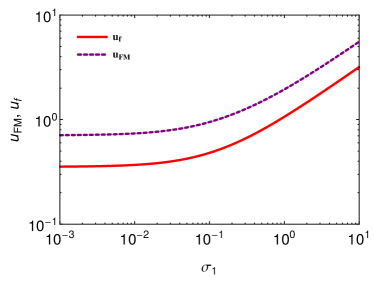
Figure 2: The four-velocities of the shock front $u_{\rm f}\,\equiv\,\overline{\gamma}_{\rm f}\overline{\beta}_{\rm f}$ and of the fastest magnetosonic mode $u_{\rm FM}\,\equiv\,\beta_{\rm FM}/\left(1-\beta_{\rm FM}^{2}\right)^{1/2}$ of the downstream plasma as a function of $\sigma_{1}$, in the ultra-relativistic limit.

For a generic wave vector $\boldsymbol{k}$ (downstream frame), the group velocity of downstream fast magnetosonic waves is $\boldsymbol{\beta_{\rm g,FM|2}}\,\equiv\,{\rm d}\omega_{\rm FM|2}/{\rm d}\boldsymbol{k}$. At given values of $(k_{y},k_{z})$, there thus exists a critical value of $k_{x,\rm c}$ above which the $x-$ component $\beta_{\rm g,FM|2,x}\,>\,\overline{\beta}_{\rm f}$. This value is shown in Fig. 3 for various values of the magnetization, as a function of $k_{z}$, assuming $k_{y}\,=\,0$; for $k_{y}\,\neq\,0$, the minimum value of $k_{x}$ is typically raised by $\,\sim\,k_{y}$ with respect to those shown in Fig. 3. As this figure shows, $k_{x,\rm c}$ becomes large at large values of $\sigma_{1}$, because the shock velocity $\overline{\beta}_{\rm f}$ becomes itself large; correspondingly, a smaller fraction of the phase space of turbulence is in contact with the shock at larger values of $\sigma_{1}$.

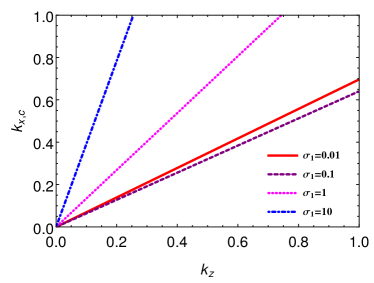
Figure 3: The minimum value of $k_{x}$ as a function of $k_{z}$ such that the downstream fast magnetosonic mode outruns the shock, for various values of $\sigma_{1}$, in the ultra-relativistic limit $\gamma_{1}\,\gg\,1$, assuming $k_{y}\,=\,0$.

Provided $\beta_{\rm g,FM|2,x}\,>\,\overline{\beta}_{\rm f}$, downstream fast magnetosonic waves thus lead to the corrugation of the shock front. In order to obtain an analytical description of the downstream turbulence in the shock vicinity, one can then solve the problem as follows: given one incoming fast magnetosonic wave outrunning the shock, represented by a particular combination of the MHD perturbations of the downstream, we determine the outgoing waves, namely one fast magnetosonic wave, two Alfvén waves, two slow magnetosonic waves and one entropy wave, as well as the shock corrugation $\delta X_{\boldsymbol{k_{\perp}}}$ (as discussed below, an assumption of stationarity then fixes $\delta V_{\boldsymbol{k_{\perp}}}\,=\,-i\,\omega_{\rm f}\delta X_{\boldsymbol{k_{\perp}}}$). In the present discussion, the upstream is assumed unperturbed, so all terms $R_{i}$, $i\,=\,1\dots 9$, vanish in Eqs. (LABEL:eq:sysbound).

In order to solve the system, we first need to specify the wave characteristics. In a stationary regime, the shock front reacts harmonically to the excitation by an incoming fast magnetosonic wave with a frequency (defined in the downstream rest frame):

$$\omega_{\rm f}\,=\,\omega_{<}-\beta_{\rm f}k_{x,<}$$ (45)

in terms of $\omega_{<}$, the frequency of the incoming fast magnetosonic wave and $k_{x,<}$ its $x$ wavenumber. Consequently, $\delta V_{\boldsymbol{k_{\perp}}}\,=\,-i\,\omega_{\rm f}\delta X_{\boldsymbol{k_{\perp}}}$. This relation is a direct expression of the Doppler effect associated to the motion of the shock front relatively to downstream: the incoming wave indeed behaves as $\delta\psi_{k,<}\,\sim\,\exp\left[-i\omega_{<}t+ik_{x,<}x+i\boldsymbol{k_{\perp}}\cdot\boldsymbol{x_{\perp}}\right]$, so that on the shock front where $x\,=x_{\rm f}\,=\,\overline{\beta}_{\rm f}t$, $\delta\psi_{k,<}\left[x_{\rm f}(t),t\right]\,\propto\,\exp\left[-i\omega_{\rm f}t+i\boldsymbol{k_{\perp}}\cdot\boldsymbol{x_{\perp}}\right]$.

Correspondingly, outgoing waves obey the relation

$$\omega_{i}-\beta_{\rm f}k_{x,i}\,=\,\omega_{\rm f}$$ (46)

where $i$ denotes the wave mode. Since $\omega_{i}$ depends on $k_{x,i}$, while $k_{y}$ and $k_{z}$ remain unchanged in the scattering process, the above equation determines $k_{x,i}$, hence $\omega_{i}$ for each mode. The various plane wave modes thus all oscillate at the same frequency on the shock surface and share the same wavenumber in the transverse directions; however, due to their differing dispersion relations, they exhibit different frequencies and $x-$ wavenumbers in the downstream plasma. Once $k_{x,<}$, $k_{y}$ and $k_{z}$ have been specified, all frequencies and $x-$ wavenumbers are determined uniquely.

Formally, the problem can be written in terms of a linear response relating the amplitude of the incoming wave to that of the outgoing waves and of the shock corrugation. Concerning the latter, one can write

$$\delta X \,=\, \int\frac{{\rm d}^{2}k_{\perp}{\rm d}\omega_{\rm f}}{(2\pi)^{3}}\delta X_{\omega_{\rm f},\boldsymbol{k_{\perp}}}e^{-i\omega_{\rm f}t+i\boldsymbol{k_{\perp}}\cdot\boldsymbol{x_{\perp}}}$$ (47)

$$\,=\, \int\frac{{\rm d}^{2}k_{\perp}{\rm d}k_{x,<}}{(2\pi)^{3}}e^{-i\omega_{\rm f}t+i\boldsymbol{k_{\perp}}\cdot\boldsymbol{x_{\perp}}}{\cal T}_{X,\boldsymbol{k}}\delta\psi_{<,\boldsymbol{k}}$$

introducing the transfer function

$${\cal T}_{X,\boldsymbol{k}}\,\equiv\,\left|\frac{{\rm d}\omega_{\rm f}}{{\rm d}k_{x,<}}\right|\,\frac{\delta X_{\omega_{\rm f},\boldsymbol{k_{\perp}}}}{\delta\psi_{<,\boldsymbol{k}}}$$ (48)

Regarding the variables describing the perturbations of the downstream plasma, one must first decompose them as a sum over the wave modes, i.e. over the eigenmodes of the system of linearized MHD equations. This is done through the matrix $\boldsymbol{{\cal M}}$, whose columns are the eigenvectors of the linearized MHD equations, as described in App. A. Recalling the notation introduced in that appendix, $\boldsymbol{\delta\xi}$ represents the set of 8 perturbation variables $\left(\delta n,\delta p,\boldsymbol{\delta\beta},\boldsymbol{\delta B}\right)$, while $\boldsymbol{\delta\psi}$ represents the set of 8 wave modes of linearized MHD; one of these 8 modes is an unphysical ghost mode carrying non-vanishing $\boldsymbol{\nabla}\cdot\boldsymbol{B}$, which must be included for a formal closure of the system, but which is not excited by the interaction of turbulence with the shock front, once the shock crossing conditions have been properly written.

For $\delta\xi_{i}\,\in\,\left\{\delta n_{2},\,\delta p_{2},\,\boldsymbol{\delta\beta}_{2},\,\boldsymbol{\delta B}_{2}\right\}$ ($i=1,\ldots,8$), the decomposition introduced in App. A takes the form

$$\delta\xi_{i}\,=\,\sum_{j}\,\int\frac{{\rm d}k_{x,j}{\rm d}k_{y}{\rm d}k_{z}}{(2\pi)^{3}}\,\,e^{-i\omega_{j}t+ik_{x,j}x+i\boldsymbol{k_{\perp}}\cdot\boldsymbol{x_{\perp}}}\boldsymbol{\mathcal{M}}_{ij}\,\delta\psi_{j,\boldsymbol{k}}$$ (49)

the sum over $j$ running over the 8 modes. It is understood here that the wave vectors and frequencies satisfy the matching conditions discussed above. Furthermore, one of the 8 modes is actually the incoming fast magnetosonic mode $\delta\psi_{<,\boldsymbol{k}}$, with $x-$ wavenumber $k_{x,<}$ and frequency $\omega_{j}\,=\,\omega_{<}$. Defining the transfer functions, with the index $j$ ranging over the wave modes

$${\cal T}_{j,\boldsymbol{k}}\,\equiv\,\left|\frac{{\rm d}k_{j,x}}{{\rm d}k_{x,<}}\right|\,\frac{\delta\psi_{j,\boldsymbol{k}}}{\delta\psi_{<,\boldsymbol{k}}}$$ (50)

with ${\cal T}_{<,\boldsymbol{k}}\,=\,1$ by definition, one can rewrite the above as

$$\delta\xi_{i} \,=\, \int\frac{{\rm d}^{2}k_{\perp}{\rm d}k_{x,<}}{(2\pi)^{3}}\,\sum_{j}e^{-i\omega_{j}t+i\boldsymbol{k_{\perp}}\cdot\boldsymbol{x_{\perp}}+ik_{x,j}x}$$ (51)

$$\quad\boldsymbol{\mathcal{M}}_{ij}\,{\cal T}_{j,\boldsymbol{k}}\delta\psi_{<,\boldsymbol{k}}$$

which provides a formal solution to the scattering problem once the transfer functions have been determined.

The system Eq. (LABEL:eq:sysbound) can be written formally as

$$\boldsymbol{\mathcal{S}}_{\boldsymbol{k_{\perp}}}\cdot\,^{\rm T}\left\{\delta X_{\boldsymbol{k_{\perp}}},\,\boldsymbol{\delta\xi}_{\boldsymbol{k_{\perp}}}\right\}\,=\,0$$ (52)

where $\boldsymbol{\mathcal{S}}_{\boldsymbol{k_{\perp}}}$ is an $8\times 9$ matrix and where the perturbations $\boldsymbol{\delta\xi}_{\boldsymbol{k_{\perp}}}$ represent the 2d Fourier transform of $\boldsymbol{\delta\xi}$ in $\boldsymbol{x_{\perp}}$, as evaluated on the unperturbed shock surface $\overline{\Phi}(x,t)\,=\,0$. The matching conditions for the wave frequencies and parallel wavenumbers guarantee that all the wave modes and $\delta X_{\boldsymbol{k_{\perp}}}$ share the same time and transverse spatial dependence on this shock surface. Using the decomposition, on the unperturbed shock surface

$$\delta\xi_{i,\boldsymbol{k_{\perp}}}\,=\,e^{-i\omega_{\rm f}t+i\boldsymbol{k_{\perp}}\cdot\boldsymbol{x_{\perp}}}\,\sum_{j}\boldsymbol{\mathcal{M}}_{ij}\delta\psi_{j,\boldsymbol{k}}$$ (53)

one can bring the system (52) into an equivalent form:

$$\boldsymbol{\mathcal{R}}_{\boldsymbol{k}}\cdot\,^{\rm T}\left\{\delta X_{\omega_{\rm f},\boldsymbol{k_{\perp}}},\,\boldsymbol{\delta\psi}_{>,\boldsymbol{k}}\right\}\,=\,\boldsymbol{R_{<,\boldsymbol{k}}}\delta\psi_{<,\boldsymbol{k}}$$ (54)

where the index _> indicates that the sum runs over the outgoing modes only. Since MHD has 8 wave modes (including one unphysical ghost mode, see App. A), and since the column associated to the incoming mode has been extracted out of $\boldsymbol{\mathcal{R}}_{\boldsymbol{k}}$ and sent into the r.h.s., the matrix $\boldsymbol{\mathcal{R}}_{\boldsymbol{k}}$ is now $8\times 8$ and the above linear problem allows to solve for $\delta X_{\boldsymbol{k_{\perp}}}$ and $\boldsymbol{\delta\psi}_{>,\boldsymbol{k_{\perp}}}$ in terms of $\delta\psi_{<,\boldsymbol{k_{\perp}}}$.

One can write an analytical solution of the above system, but given the large rank of the matrix, its inverse cannot be written in a compact way. For these reasons, we provide in the following direct estimates of the solutions for various cases of interest.

3.1 Results

In Fig. 4, we show a contour plot of the transfer functions for the various modes, in the plane $(k_{x,<},k_{y})$, for $\sigma_{1}\,=\,0.1$ and $\gamma_{1}\,=\,10^{4}$ (representative of the ultra-relativistic limit $\gamma_{1}\,\gg\,1$). In this figure, $k_{z}\,=\,10^{-3}$; units for wavenumbers are arbitrary, as the problem of corrugation of a planar shock front does not possess an intrinsic scale. For the two slow magnetosonic and for the two Alfvén modes, the transfer functions have been respectively added together.

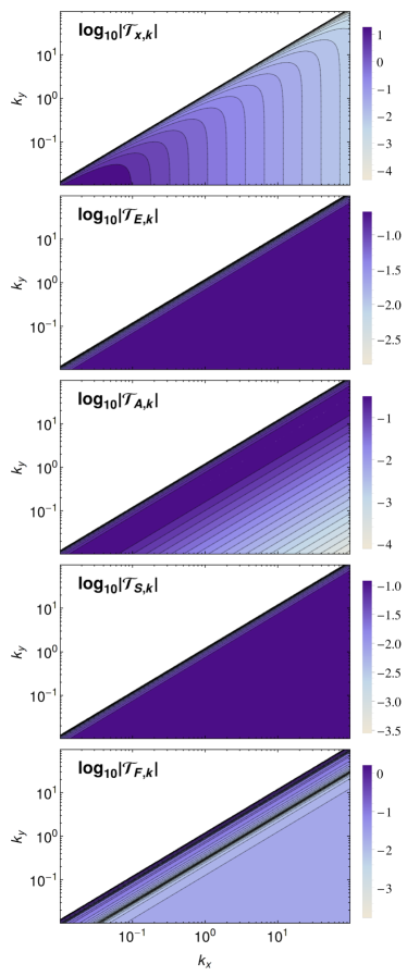
Figure 4: Contour plots of the transfer functions for $\sigma_{1}\,=\,0.1$, $\gamma_{1}\,=\,10^{4}$ (ultra-relativistic limit) in the 2D-plane $(k_{x},\,k_{y})$; $k_{z}\,=\,10^{-3}$ everywhere here. The symbols are as follows: $\mathcal{T}_{X,\boldsymbol{k}}$ represents the response of the shock corrugation amplitude, and indices _E, _A, _S and _F respectively refer to the entropy mode, the two Alfvén modes (sum of the two responses), the two slow magnetosonic modes (also summed) and the reflected fast magnetosonic mode.

Figure 5 presents a contour plot equivalent to that shown in Fig. 4, but for perturbations along the magnetic field; i.e., $k_{y}\,=\,10^{-3}$ and the contour is shown in the $(k_{x,<},k_{z})$ plane.

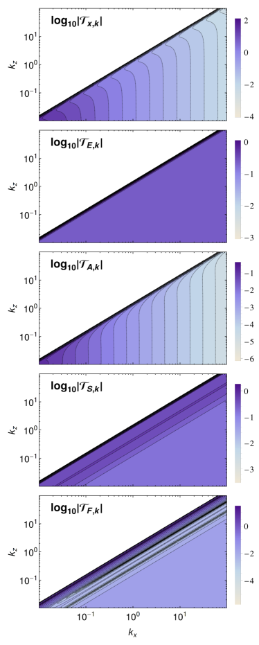
Figure 5: Contour plots of the transfer functions for $\sigma_{1}\,=\,0.1$, $\gamma_{1}\,=\,10^{4}$ (ultra-relativistic limit) in the 2D-plane $(k_{x},\,k_{z})$; $k_{y}\,=\,10^{-3}$ everywhere here.

A general trend observed in these figures and in a more systematic survey is that the incoming fast magnetosonic mode is converted in roughly similar proportions in the various outgoing modes. At large values of $k_{x}$, in particular $k_{x}\,\gg\,k_{y},\,k_{z}$, the transfer function for the shock corrugation amplitude scales as $1/k_{x}$, with typically $\left|\mathcal{T}_{X,\boldsymbol{k}}\right|\,\sim\,{\mathcal{O}}(1)k_{x}^{-1}$. This scaling appears as a natural consequence of the scale invariance of the problem at hand – there being no natural length scale associated to the physics of a planar infinite shock front in the MHD limit – once one recalls that $\left|\mathcal{T}_{X,\boldsymbol{k}}\right|$ carries the dimensions of a length scale, because $\delta X$ is a length scale while $\delta\psi_{<}$ is dimensionless. The prefactor is typically of order unity, although it depends somewhat on the nature of the incoming wave and on the magnetization of the upstream plasma.

4 Transmission of upstream turbulence

This Section discusses the transmission of upstream turbulence through the shock. For the sake of simplicity, this discussion is restricted to the transmission of entropy and Alfvén waves, for which the Riemann invariants of the linearized MHD system of a streaming plasma can be written in a compact way. In principle, the problem can be generalized directly to include the transmission of upstream magnetonic waves. However, the analysis is here carried out in the rest frame of the downstream plasma, with respect to which the upstream plasma is drifting at relativistic speeds. In this case, the Riemann invariants associated to magnetosonic wave modes take quite complicated expressions, making the algebra cumbersome. The following therefore focuses on entropy and Alfvén waves; a numerical example of the impact of incoming fast magnetosonic waves will nevertheless be provided in Fig. 9.

The procedure follows that of Sec. 3. One first decomposes the drifting upstream turbulence in its eigenmodes in Fourier space. The entropy mode is characterized by $\delta n_{1}\,=\,n_{1}\delta\psi_{\rm E1}$ and all other perturbations $\boldsymbol{\delta\beta}_{1}\,=\,\boldsymbol{\delta B}_{1}\,=\,0$ (note that $\delta p_{1}$ is no longer a perturbation variable since the upstream plasma is considered cold). In the rest frame of the upstream plasma, the eigenfrequency is $\omega_{\rm E1|u}\,=\,0$, so that in the downstream frame: $\omega_{\rm E1}\,=\,\beta_{1}k_{x}$.

In terms of the perturbation amplitude $\delta\psi_{\rm A1}$, the Alfvén modes are characterized by:

$$\delta n_{1} \,=\, \delta\beta_{1z}\,=\,0,$$

$$\delta\beta_{1x} \,=\, \frac{1}{\gamma_{1}^{2}}\delta\psi_{\rm A1}\,$$

$$\delta\beta_{1y} \,=\, \frac{\beta_{1}\omega_{\rm A1}-k_{x}}{k_{y}}\delta\psi_{\rm A1}\,$$

$$\delta B_{1x} \,=\, -\frac{k_{z}}{\gamma_{1}^{2}\left(\omega_{\rm A1}-\beta_{1}k_{x}\right)}\delta\psi_{\rm A1}\,$$

$$\delta B_{1y} \,=\, -\frac{k_{z}\left(\beta_{1}\omega_{\rm A1}-k_{x}\right)}{k_{y}\left(\omega_{\rm A1}-\beta_{1}k_{x}\right)}\delta\psi_{\rm A1}\,$$

$$\delta B_{1z} \,=\, \beta_{1}\delta\psi_{\rm A1}$$ (55)

with frequency: $\omega_{\rm A1}\,=\,\beta_{1}k_{x}\pm\beta_{\rm A1}k_{z}/\gamma_{1}^{2}$. It is easy to verify that one recovers the corresponding eigenmode for a plasma at rest, Eq. (LABEL:eq:eigenvec), in the limit $\beta_{1}\,\rightarrow\,0$, $\gamma_{1}\,\rightarrow\,1$.

The frequency of the corrugation amplitude $\delta X_{\boldsymbol{k_{\perp}}}$ is determined by the matching:

$$\omega_{\rm f}\,=\,\omega_{1}-\overline{\beta}_{\rm f}k_{x}$$ (56)

with $\omega_{1}\,=\,\omega_{\rm E1}$ or $\omega_{\rm A1}$ depending on the source of the perturbations entering the shock. The corrugations induced on the shock are then converted into downstream outgoing perturbations. The frequency $\omega_{i}$ and wavenumbers $k_{x,i}$ of these modes are determined as previously in terms of $\omega_{\rm f}$, of course.

There are now six outgoing modes: 1 entropy, 2 Alfvén, 2 slow magnetosonic and 1 fast magnetosonic mode. That only one fast magnetosonic mode is excited is a non-trivial result by itself, which deserves some discussion. At a given value of $\omega_{\rm f}$ – equivalently, at a given value of the $x-$ component $k_{x}$ of the incoming perturbation – one can find the values of $k_{x,i}$ of the magnetosonic waves which satisfy the frequency matching condition Eq. (46) by solving the equation:

$$\left(\omega_{\rm f}+\overline{\beta}_{\rm f}k_{x,i}\right)^{4} - \left(\beta_{\rm FM}^{2}k^{2}+\beta_{\rm A}^{2}c_{\rm s}^{2}k_{z}^{2}\right)\left(\omega_{\rm f}+\overline{\beta}_{\rm f}k_{x,i}\right)^{2}+$$ (57)

$$\quad\beta_{\rm A}^{2}c_{\rm s}^{2}k^{2}k_{z}^{2}\,=\,0$$

which is nothing else but the dispersion relation of magnetosonic waves, with the frequency replaced by $\omega_{\rm f}+\overline{\beta}_{\rm f}k_{x,i}$; it is understood here that $k^{2}=k_{x,i}^{2}+k_{y}^{2}+k_{z}^{2}$. This quartic equation has at most four real solutions, then corresponding to two fast and two slow magnetosonic waves. One finds that there exists a critical value of the incoming $k_{x}$ (for $k_{x}\,>\,0$), below which the above equation has two real solutions and a pair of complex conjugate solutions, and above which the equation has four real solutions. At the critical value of $k_{x}$, written $k_{x,\rm c}$ in the following, the group velocity of the downstream fast magnetosonic wave is very close or equal to the shock velocity, $\beta_{{\rm g,FM},x}\,\simeq\,\overline{\beta}_{\rm f}$. For $k_{x}\,>\,k_{x,\rm c}$, one of the fast magnetosonic waves has a group velocity in excess of $\overline{\beta}_{\rm f}$, while the other has a group velocity smaller than $\overline{\beta}_{\rm f}$. Therefore, in this case, only one fast magnetosonic wave (the slower) can be excited by the corrugation. For $k_{x}\,<\,k_{x,\rm c}$, one of the complex solutions has a positive imaginary part, which corresponds to an unphysical solution with unbounded amplitude towards far downstream ($x\,\rightarrow\,-\infty$). In this case, we thus set this wave to zero, and retain only the wave with negative imaginary part of $k_{x,i}$, which physically describes a mode localized on the shock front.

Formally, the problem is then written as in the previous Section, see Eq. (54), except that the source of corrugation is no longer the downstream fast magnetosonic mode, but rather the incoming upstream perturbation, as indicated by the r.h.s. of Eq. (LABEL:eq:sysbound):

$$\boldsymbol{\mathcal{R}}_{\boldsymbol{k}}\cdot\,^{\rm T}\left\{\delta X_{\omega_{\rm f},\boldsymbol{k_{\perp}}},\,\boldsymbol{\delta\psi}_{>,\boldsymbol{k}}\right\}\,=\,\boldsymbol{R}_{1,\boldsymbol{k}}\delta\psi_{1,\boldsymbol{k}}$$ (58)

with $\boldsymbol{R}_{1,\boldsymbol{k}}$ determined by Eq. (28) and the decomposition of the perturbations $\delta n_{1,\boldsymbol{k_{\perp}}}$ etc. in terms of $\delta\psi_{1,\boldsymbol{k}}$, for each of the two cases studied here, $\delta\psi_{1,\boldsymbol{k}}\,=\,\delta\psi_{{\rm E1},\boldsymbol{k}}$ or $\delta\psi_{{\rm A1},\boldsymbol{k}}$.

One can then define the transfer functions

$${\mathcal{T}}_{X,\boldsymbol{k}}\,\equiv\,\left|\frac{{\rm d}\omega_{\rm f}}{{\rm d}k_{x,<}}\right|\,\frac{\delta X_{\omega_{\rm f},\boldsymbol{k_{\perp}}}}{\delta\psi_{1,\boldsymbol{k}}}$$ (59)

and

$${\cal T}_{j,\boldsymbol{k}}\,\equiv\,\left|\frac{{\rm d}k_{j,x}}{{\rm d}k_{x,<}}\right|\,\frac{\delta\psi_{j,\boldsymbol{k}}}{\delta\psi_{1,\boldsymbol{k}}}$$ (60)

as before, now expressed relatively to the incoming upstream perturbation.

If perturbations are sourced by upstream fluctuations, one finds that there exist values of $(k_{x},k_{y},k_{z})$ for which ${\rm Det}\,\boldsymbol{\mathcal{R}}_{\boldsymbol{k}}\,=\,0$, which correspond to a resonant response of the shock corrugation to the incoming perturbation, with formally infinite corrugation amplitude. This result stands in contrast with the case studied in the previous Section, for which one could not find values of $(k_{x},k_{y},k_{z})$ which lead to a vanishing determinant; the difference lies of course in the relationship which ties $\omega_{\rm f}$ to $k_{x,<}$, and which differs between those two cases.

4.1 Non-resonant response

As in Sec. 3, we show here the transfer functions for the response to the excitation by incoming entropy and Alfvén modes. Given the large dimensionality of the parameter space, we restrict these plots to the region in which $k_{y}\,=\,k_{z}$, to $\sigma_{1}\,=\,0.1$ and to the ultra-relativistic limit $\gamma_{1}\,\gg\,1$ (for practical matters, $\gamma_{1}\,=\,10^{4}$ here). The transmission of entropy modes is shown in Fig. 6, while the transmission of Alfvén modes is shown in Fig. 7.

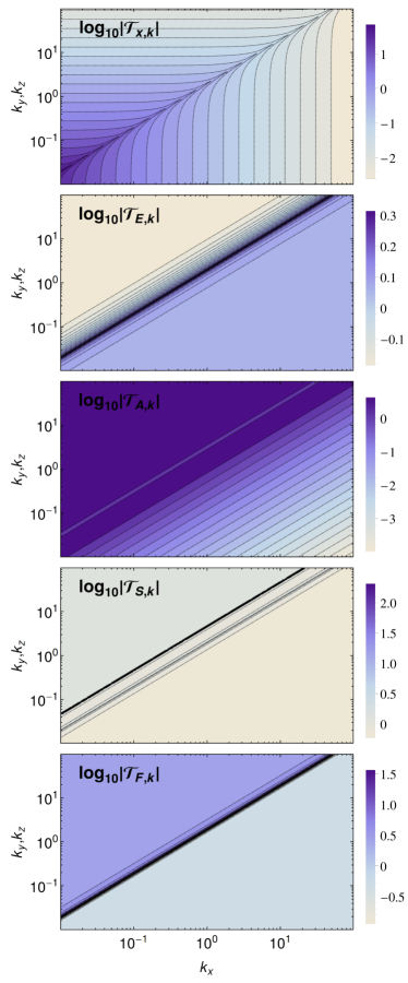
Figure 6: Contour plots of the transfer functions for $\sigma_{1}\,=\,0.1$, $\gamma_{1}\,=\,10^{4}$ (ultra-relativistic limit) in the 2D-plane $(k_{x},\,k_{y})$ with $k_{z}\,=\,k_{y}$ everywhere here, for an incoming entropy mode

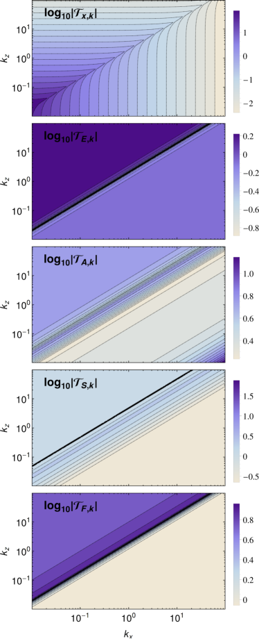
Figure 7: Contour plots of the transfer functions for $\sigma_{1}\,=\,0.1$, $\gamma_{1}\,=\,10^{4}$ (ultra-relativistic limit) in the 2D-plane $(k_{x},\,k_{y})$ with $k_{z}\,=\,k_{y}$ everywhere here, for an incoming Alfvén wave.

These curves reveal a ridge along which the amplification takes large values; this resonant response is analyzed in greater detail in the following Sec. 4.2. In other parts of parameter space, the response of the shock front to the incoming perturbation is of order unity, meaning $\left|k\delta X_{\boldsymbol{k}}\right|\,\sim\,{\cal O}(1)\,\delta\psi_{1}$, leading to the non-linear regime of corrugation if the incoming amplitude is of order unity.

4.2 Resonant response

As discussed above, at certain locations of $\boldsymbol{k}$, the determinant of the response matrix of the shock corrugation and outgoing wave amplitudes takes small or even vanishing values, leading to a large amplification of the incoming perturbation in the present linear approximation. For all cases surveyed, it was found that, for a given pair $(k_{y},k_{z})$, there is at most one resonant value, written $k_{x,\rm r}$ with $k_{x,\rm r}\,\simeq\,k_{x,\rm c}$ to very good accuracy. The latter remark motivates the following interpretation: as $k_{x}\,\rightarrow\,k_{x,\rm c}$, the outgoing fast magnetosonic wave rides along with the shock front, because its group velocity matches $\overline{\beta}_{\rm f}$; therefore, the large corrugation and consequent amplification of downstream modes follow from the build-up of the fast magnetosonic mode energy on the shock.

On a root of ${\rm Det}\,\boldsymbol{\mathcal{R}}_{\boldsymbol{k}}$, all downstream perturbations diverge. In order to illustrate the effect of such a resonant response, we plot in Fig. 7 the $\delta B_{z}$ perturbation, assuming an incoming perturbation $\delta\psi_{{\rm A1},\boldsymbol{k}}\,=\,0.1$ (hence $|\delta B_{z,1,\boldsymbol{k_{\perp}}}|\,\simeq\,0.1$). Here, $k_{x}\,\simeq\,0.3308$ ($-0.01\,$% away from the actual root), $k_{y}\,=\,0.001$, $k_{z}\,=\,1.$, $\sigma_{1}\,=\,0.1$ and $\gamma_{1}\,=\,10^{4}$. The contours are spaced logarithmically; note the amplification by a factor $\gtrsim\,80$ of the downstream perturbation. For these values, one finds a corrugation amplitude $\left|\delta X_{\boldsymbol{k_{\perp}}}\right|\,\sim\,150$, well into the non-linear regime; Fig. 8 should thus be considered as an illustration, in the framework of the linear approximation.

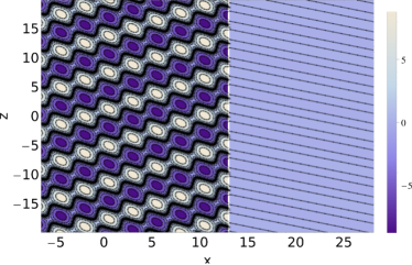
Figure 8: Snapshot contour plot of the perturbation $\delta B_{z}$ in configuration space, in the $(x,y)$ plane. The shock front lies at $x\,=\,13$. An Alfvén perturbation with amplitude $\delta\psi_{{\rm A1},\boldsymbol{k}}\,=\,0.1$ enters the shock from upstream ($x\,>\,13$) and seeds corrugation; the amplitude of the outgoing mode reaches here $|\delta B_{z,\boldsymbol{k_{\perp}}}|\,\sim\,9$. Parameters are: $\sigma_{1}\,=\,0.1$, $\gamma_{1}\,=\,10^{4}$, $k_{x}\,=\,0.33$, $k_{y}\,=\,0.001$, $k_{z}\,=\,1$.

Our study of parameter space reveals that the response at $k_{x}\,\rightarrow\,k_{x,\rm r}$ dominates over that at other wavenumbers. In order to illustrate this point, we show in Fig. 9 the modulus squared of the transfer function for the corrugation amplitude as a function of $k_{x}$, for several cases. This quantity relates the power spectrum of corrugation to the power spectrum of the incoming turbulence, through

$${\mathcal{P}}_{\delta X,\boldsymbol{k}}\,=\,\left|{\mathcal{T}}_{X,\boldsymbol{k}}\right|^{2}{\mathcal{P}}_{1,\boldsymbol{k}}$$ (61)

with

$$\left\langle\delta X^{2}\right\rangle\,=\,\int\frac{{\rm d}^{3}k}{(2\pi)^{3}}{\mathcal{P}}_{\delta X,\boldsymbol{k}}$$ (62)

and similarly for the incoming wave in terms of $\left\langle\delta\psi_{1}^{2}\right\rangle$. Figure 9 assumes an Alfvén wave in the incoming state.

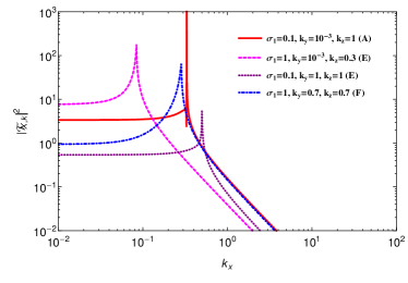
Figure 9: Slice of the transfer function for various waves as indicated, $\gamma_{1}\,=\,10^{4}$ (ultra-relativistic limit) as a function of $k_{x}$; (A) refers to Alfvén waves, (E) to entropy waves and (F) to fast magnetosonic waves.

The resonant behavior at $k_{x,\rm r}$ is clear in the above figure. At larger values of $k_{x}$, in particular $k_{x}\,\gg\,k_{y},\,k_{z}$, one recovers the scaling $\left|\mathcal{T}_{X,\boldsymbol{k}}\right|\,\sim\,{\mathcal{O}}(1)k_{x}^{-1}$ observed in Sec. 3.

Figure 9 also reveals that the magnitude of the amplification at the resonant value of $k_{x}$ depends on the parameters, in particular $k_{y},\,k_{z}$ and $\sigma_{1}$. One typically observes that for $k_{y}\,\gtrsim\,k_{z}$ or $\sigma_{1}\,\gtrsim\,0.3$, the determinant does not vanish at $k_{x}\,\rightarrow\,k_{x,\rm r}$ but takes a minimum value, nevertheless leading to large but finite amplification of the incoming wave, while at $k_{y}\,\ll\,k_{z}$ and $\sigma_{1}\,\lesssim\,0.3$, actual roots of ${\rm Det}\,\boldsymbol{\mathcal{R}}_{\boldsymbol{k}}\,=\,0$ exist, with correspondingly infinite amplification.

For the latter case, a careful study of the transfer function in the vicinity of the root, $k_{x}\,=\,k_{x,\rm r}(1+\epsilon)$, reveals that

$$\left|\mathcal{T}_{X,\boldsymbol{k}}\right|\,\propto\,\frac{1}{\left|\epsilon\right|}$$ (63)

which indicates that the power spectrum of corrugation diverges as $1/\epsilon^{2}$ at the resonance. The present linear theory thus strongly suggests that these resonances should dominate the response of the shock to the incoming turbulence. One should nevertheless recall that this analysis assumes a stationary upstream turbulence, and that in the presence of modes with finite damping coefficients, the influence of the above narrow resonances might be diminished. We defer to a future work a detailed study of these resonances and their consequences for the phenomenology of astrophysical shock waves.

5 Conclusions

This paper has provided a general analysis of the corrugation of relativistic magnetized (fast) shock waves induced by the interaction of the shock front with moving disturbances. Two cases have been analyzed, depending on the nature of these disturbances: whether they are fast magnetosonic waves originating from the downstream side of the shock front, outrunning the shock, or whether they are eigenmodes of the upstream plasma.

Working to first order in the perturbations of the flows, on both sides of the shock front, as in the amplitude of corrugation $\delta X$ of the shock front, we have provided transfer functions relating the amplitude of the outgoing wave modes to the amplitude of the incoming wave, thus developing a linear response theory for the corrugation. We have then provided estimates of these transfer functions for different cases of interest.

One noteworthy result is that the front generically responds with $|\partial\delta X|\,\sim\,{\cal O}(1)\delta\psi_{<}$, where $\delta\psi_{<}$ represents the amplitude of the incoming wave, the partial derivative being taken along $t$, $y$ or $z$. The corrugation remains linear as long as $|\partial\delta X|\,\ll\,1$, therefore the present analysis is restricted to small amplitude incoming waves. Interestingly, however, the extrapolation of the present results indicates that non-linear corrugation can be achieved in realistic situations.

In this respect, we have obtained an original solution for the equations of shock crossing, in the non-perturbative regime; this solution allows to calculate the amplitude of fluctuations in density, pressure, velocity and magnetic field components at all locations (and all times) on a shock surface which is arbitrarily rippled in the $y-$ direction, but smooth along the background magnetic field.

Furthermore, when corrugation is induced by upstream wave modes, we find that there exist resonant wavenumbers $\boldsymbol{k}$ where the linear response becomes large or even formally infinite, leading to large or formally infinite amplification of the incoming wave amplitude and of the shock corrugation. For a given pair $(k_{y},k_{z})$, there exists one such resonance in $k_{x}$ for the incoming mode, corresponding to the value at which the outgoing fast magnetosonic mode moves as fast as the shock front. The physics of shock waves interacting with turbulence containing such resonant wavenumbers should be examined with dedicated numerical simulations able to probe the deep non-linear regime, as the structure of the turbulence produced by the corrugation may have profound consequences for our understanding of astrophysical magnetized relativistic shock waves and their phenomenology.

Appendix A Wave modes in relativistic MHD

The dynamics of the plasma is governed by the MHD equations:

$$\partial_{\mu}\left(nu^{\mu}\right) \,=\, 0$$ (A1)

$$\partial_{\mu}T^{\mu\nu} \,=\, 0$$ (A2)

$$\partial_{\mu}\,^{\star}F^{\mu\nu} \,=\, 0$$ (A3)

$$\partial_{\mu}\,F^{\mu\nu} \,=\, 4\pi j^{\nu}$$ (A4)

The various quantities entering these equations are defined in Sec. 2.1.

The wave modes of an unbounded plasma can be obtained as usual by linearizing these equations around an unperturbed state characterized by uniform energy density, pressure and density, and regular magnetic field, assumed oriented along $\boldsymbol{z}$: $\boldsymbol{\overline{B}}=B_{z}\boldsymbol{z}$. The sound and (relativistic) Alfvén velocities are defined according to:

$$c_{\rm s}^{2}\,=\,\hat{\gamma}\frac{p}{w},\quad\beta_{\rm A}^{2}\,=\,\frac{\overline{B}^{2}}{4\pi W}$$ (A5)

and $\hat{\gamma}$ is the polytropic index.

As is well-known, the linearized equations and their solutions are characterized, in Fourier space, by 8 perturbation variables $\boldsymbol{\delta\xi}_{\boldsymbol{k}}\,=\,\left(\delta n_{\boldsymbol{k}},\delta p_{\boldsymbol{k}},\boldsymbol{\delta\beta}_{\boldsymbol{k}},\boldsymbol{\delta B}_{\boldsymbol{k}}\right)$. These perturbations define 8 modes: one entropy mode (indexed _E), two Alfvén modes (indexed _A), two slow magnetosonic modes (indexed _SM), two fast magnetosonic modes (indexed _FM), and one non-physical ghost mode carrying non-vanishing $\boldsymbol{\nabla}\cdot\boldsymbol{B}$ (not discussed in the following). The corresponding frequencies of these various modes are:

$$\omega_{\rm E} \,=\, 0,$$

$$\omega_{\rm A} \,=\, \pm\beta_{\rm A}k_{z},$$

$$\omega_{\rm SM} \,=\, \pm\frac{1}{\sqrt{2}}\biggl{\{}\beta_{\rm FM}^{2}k^{2}+\beta_{\rm A}^{2}c_{\rm s}^{2}k_{z}^{2}-\biggl{[}\left(\beta_{\rm FM}^{2}k^{2}+\beta_{\rm A}^{2}c_{\rm s}^{2}k_{z}^{2}\right)^{2}-4\beta_{\rm A}^{2}c_{\rm s}^{2}k_{z}^{2}k^{2}\biggr{]}^{1/2}\biggr{\}}^{1/2},$$

$$\omega_{\rm FM} \,=\, \pm\frac{1}{\sqrt{2}}\biggl{\{}\beta_{\rm FM}^{2}k^{2}+\beta_{\rm A}^{2}c_{\rm s}^{2}k_{z}^{2}+\biggl{[}\left(\beta_{\rm FM}^{2}k^{2}+\beta_{\rm A}^{2}c_{\rm s}^{2}k_{z}^{2}\right)^{2}-4\beta_{\rm A}^{2}c_{\rm s}^{2}k_{z}^{2}k^{2}\biggr{]}^{1/2}\biggr{\}}^{1/2}$$

which take the same functional form as in non-relativistic MHD. The velocity $\beta_{\rm FM}$ is defined by: $\beta_{\rm FM}\,\equiv\,\left(\beta_{\rm A}^{2}+c_{\rm s}^{2}-\beta_{\rm A}^{2}c_{\rm s}^{2}\right)^{1/2}$. For convenience, we also define $c_{+}\,\equiv\,\left(\beta_{\rm A}^{2}+c_{\rm s}^{2}\right)^{1/2}$.

Fast magnetosonic waves thus propagate at a phase velocity $|\omega_{\rm FM}/k|$, which ranges from ${\rm max}\left(\beta_{\rm A},c_{\rm s}\right)$ at $k_{x}\,=\,k_{y}\,=\,0$ to $\beta_{\rm FM}$ at $k_{z}\,=\,0$. Slow magnetosonic waves propagate at a phase velocity $|\omega_{\rm SM}/k|$, which ranges from $0$ at $k_{z}\,=\,0$ to ${\rm min}\left(\beta_{\rm A},c_{\rm s}\right)$ at $k_{\perp}\,=\,0$. For further details, see Goedbloed et al. (2010) or Keppens & Meliani (2008).

The various MHD modes can be decomposed over the perturbation variables as follows:

$$\boldsymbol{\delta\xi}_{{\rm E},\boldsymbol{k}} \,=\, \left\{n,0,0,0,0,0,0,0\right\}\delta\psi_{{\rm E},\boldsymbol{k}}$$

$$\boldsymbol{\delta\xi}_{{\rm A},\boldsymbol{k}} \,=\, \left\{0,0,\frac{k_{y}\omega_{\rm A}}{k_{x}k_{z}},-\frac{\omega_{\rm A}}{k_{z}},0,-\frac{k_{y}}{k_{x}}B_{z},B_{z},0\right\}\delta\psi_{{\rm A},\boldsymbol{k}}$$

$$\boldsymbol{\delta\xi}_{{\rm M},\boldsymbol{k}} \,=\, \left\{\frac{\omega_{\rm M}^{2}-\beta_{\rm A}^{2}k^{2}}{c_{\rm s}^{2}\left(1-\beta_{\rm A}^{2}\right)\left(k_{x}^{2}+k_{y}^{2}\right)}n,\frac{\omega_{\rm M}^{2}-\beta_{\rm A}^{2}k^{2}}{k_{x}^{2}+k_{y}^{2}}W,\frac{\omega_{\rm M}k_{x}}{k_{x}^{2}+k_{y}^{2}},\frac{\omega_{\rm M}k_{y}}{k_{x}^{2}+k_{y}^{2}},\frac{c_{\rm s}^{2}\omega_{\rm M}k_{z}}{\omega_{\rm M}^{2}-c_{\rm s}^{2}k_{z}^{2}},-\frac{k_{x}k_{z}}{k_{x}^{2}+k_{y}^{2}}B_{z},-\frac{k_{y}k_{z}}{k_{x}^{2}+k_{y}^{2}}B_{z},B_{z}\right\}\delta\psi_{{\rm M},\boldsymbol{k}}$$

where the subscript _M indicates that this applies separately for all four magnetosonic modes with corresponding frequency $\omega_{\rm M}$. For completeness, one should include the ghost mode with $\boldsymbol{\delta\xi}_{{\rm G},\boldsymbol{k}}\,=\,\left\{0,0,0,0,0,k_{x}B_{z},k_{y}B_{z},k_{z}B_{z}\right\}\delta\psi_{{\rm G},\boldsymbol{k}}$ and frequency $\omega_{\rm G}\,=\,0$.

Given a set of modes, each possibly carrying a different $\omega_{i}$ and $k_{x,i}$ (but assuming that they all share a same $(k_{y},k_{z})$ as in Sec. 3), one can use the above decomposition to relate the set of perturbation variables in configuration space to the 8 characteristics of the linearized MHD system:

$$\delta\xi_{i}\,=\,\sum_{j}\,\int\frac{{\rm d}k_{x,j}{\rm d}k_{y}{\rm d}k_{z}}{(2\pi)^{3}}\,e^{-i\omega_{j}t+ik_{x,j}x+i\boldsymbol{k_{\perp}}\cdot\boldsymbol{x_{\perp}}}\boldsymbol{\mathcal{M}}_{ij}\delta\psi_{j}$$ (A8)

introducing the $8\times 8$ matrix $\boldsymbol{\mathcal{M}}$, whose columns are given by the 8 brackets of the r.h.s. of Eq. (LABEL:eq:eigenvec) including the ghost mode, with possibly different wavenumbers $k_{x}$ in each separate mode.

References

- Achterberg & Blandford (1986) Achterberg, A., & Blandford, R. D. 1986, Month. Not. Roy. Astron. Soc., 218, 551
- Anile & Russo (1986) Anile, A. M., & Russo, G. 1986, Physics of Fluids, 29, 2847
- Bates & Montgomery (2000) Bates, J. W., & Montgomery, D. C. 2000, Physical Review Letters, 84, 1180
- Begelman & Kirk (1990) Begelman, M. C., & Kirk, J. G. 1990, Astrophys. J., 353, 66
- Bykov et al. (2012) Bykov, A., Gehrels, N., Krawczynski, H., et al. 2012, Sp. Sc. Rev., 173, 309
- Bykov (1982) Bykov, A. M. 1982, Soviet Astronomy Letters, 8, 320
- Bykov & Treumann (2011) Bykov, A. M., & Treumann, R. A. 2011, Astron. Astrophys. Rev., 19, 42
- Chen et al. (2015) Chen, H., Fiuza, F., Link, A., et al. 2015, Phys. Rev. Lett., 114, 215001
- D’Iakov (1958) D’Iakov, S. P. 1958, Soviet Journal of Experimental and Theoretical Physics, 6, 739
- Drake & Gregori (2012) Drake, R. P., & Gregori, G. 2012, Astrophys. J., 749, 171
- Gardner & Kruskal (1964) Gardner, C. S., & Kruskal, M. D. 1964, Physics of Fluids, 7, 700
- Goedbloed et al. (2010) Goedbloed, J., Keppens, R., & Poedts, S. 2010, Advanced Magnetohydrodynamics: With Applications to Laboratory and Astrophysical Plasmas (Cambridge University Press)
- Huntington et al. (2015) Huntington, C. M., Fiuza, F., Ross, J. S., et al. 2015, Nat. Phys., 11, 173
- Kennel & Coroniti (1984) Kennel, C. F., & Coroniti, F. V. 1984, ApJ, 283, 694
- Keppens & Meliani (2008) Keppens, R., & Meliani, Z. 2008, Physics of Plasmas, 15, 102103
- Kirk & Duffy (1999) Kirk, J. G., & Duffy, P. 1999, Journal of Physics G Nuclear Physics, 25, R163
- Kontorovich (1958) Kontorovich, V. M. 1958, Soviet Journal of Experimental and Theoretical Physics, 6, 1179
- Kuramitsu et al. (2011) Kuramitsu, Y., Sakawa, Y., Morita, T., et al. 2011, Physical Review Letters, 106, 175002
- Landau & Lifshitz (1987) Landau, L. D., & Lifshitz, E. M. 1987, Fluid Mechanics, Second Edition: Volume 6 (Course of Theoretical Physics), 2nd edn., Course of theoretical physics / by L. D. Landau and E. M. Lifshitz, Vol. 6 (Butterworth-Heinemann)
- Lessen & Deshpande (1967) Lessen, M., & Deshpande, N. V. 1967, Physics of Fluids, 10, 782
- Lobet et al. (2015) Lobet, M., Ruyer, C., Debayle, A., et al. 2015, Physical Review Letters, 115, 215003
- Lyutikov et al. (2012) Lyutikov, M., Balsara, D., & Matthews, C. 2012, Month. Not. Roy. Astron. Soc., 422, 3118
- Majorana & Anile (1987) Majorana, A., & Anile, A. M. 1987, Physics of Fluids, 30, 3045
- McKenzie & Westphal (1970) McKenzie, J. F., & Westphal, K. O. 1970, Physics of Fluids, 13, 630
- Moiseev & Sagdeev (1963) Moiseev, S. S., & Sagdeev, R. Z. 1963, Journal of Nuclear Energy, 5, 43
- Park et al. (2012) Park, H.-S., Ryutov, D., Ross, J., et al. 2012, High Energy Density Physics, 8, 38
- Park et al. (2015) Park, H.-S., Huntington, C. M., Fiuza, F., et al. 2015, Phys. Plasmas, 22, 056311
- Sironi et al. (2015) Sironi, L., Keshet, U., & Lemoine, M. 2015, Sp. Sc. Rev., 191, 519
- Tsintsadze et al. (1997) Tsintsadze, L. N., Chilashvili, M. G., Shukla, P. K., & Tsintsadze, N. L. 1997, Physics of Plasmas, 4, 3923