New solutions for non-Abelian cosmic strings

Abstract

We study the properties of classical vortex solutions in a non-Abelian gauge theory. A system of two adjoint Higgs fields breaks the $\mathrm{SU}(2)$ gauge symmetry to $Z_{2}$, producing ’t Hooft-Polyakov monopoles trapped on cosmic strings, termed beads; there are two charges of monopole and two degenerate string solutions. The strings break an accidental discrete $Z_{2}$ symmetry of the theory, explaining the degeneracy of the ground state. Further symmetries of the model, not previously appreciated, emerge when the masses of the two adjoint Higgs fields are degenerate. The breaking of the enlarged discrete symmetry gives rise to additional string solutions and splits the monopoles into four types of ‘semipole’: kink solutions that interpolate between the string solutions, classified by a complex gauge invariant magnetic flux and a $Z_{4}$ charge. At special values of the Higgs self-couplings, the accidental symmetry broken by the string is continuous, giving rise to supercurrents on the strings. The $\mathrm{SU}(2)$ theory can be embedded in a wide class of Grand Unified Theories, including $\mathrm{SO}(10)$. We argue that semipoles and supercurrents are generic on GUT strings.

Cosmic strings Kibble (1976) are line-like concentrations of energy and tension which may have been created in the early universe (for reviews see Hindmarsh and Kibble (1995); Vilenkin and Shellard (2000); Copeland et al. (2011); Hindmarsh (2011)). They may be either classical vortex solutions in a field theory with spontaneously broken symmetries Kibble (1976), or fundamental objects in a string theory Witten (1985a); Sarangi and Tye (2002); Copeland et al. (2004). The form of the Standard Model as a theory of gauge (local) symmetries spontaneously broken at a scale of O(100) GeV, and its inability to account for dark matter and the baryon asymmetry of the universe, motivates the study of extensions to the Standard Model with further spontaneously broken gauge symmetries.

The simplest such extension, a theory with an extra gauged $\mathrm{U}(1)$ symmetry, has cosmic string solutions in the form of Nielsen-Olesen vortices Nielsen and Olesen (1973) in the Abelian Higgs model. These Abelian Higgs strings have been extensively studied numerically in order to establish the dynamics of their formation and evolution in the early universe, and the ensuing observational predictions Laguna and Matzner (1989); Vincent et al. (1998); Moore et al. (2002); Bevis et al. (2007, 2010). Theories with two broken $\mathrm{U}(1)$ gauge symmetries, in which strings can form bound states and junctions, have been studied numerically as a model for cosmic fundamental strings Urrestilla and Vilenkin (2008); Lizarraga and Urrestilla (2016).

Other spontaneously broken symmetries produce strings. Indeed, if a compact non-abelian gauge group $G$ is broken to a subgroup $H,$ strings are guaranteed if the manifold $G/H$ is non-simply connected Kibble (1976). If $G$ is itself simply connected, it can be shown that $G/H$ is non-simply connected if and only if $H$ is disconnected. The simplest class of examples is the symmetry-breaking $\mathrm{SU}(2)\to Z_{N}$, and string network simulations have been performed in theories with broken global symmetries and $N=3$ Hindmarsh and Saffin (2006).

In the absence of global symmetries and accidental degeneracies, $G/H$ is isomorphic to the vacuum manifold of the theory. If $G$ is embedded in a larger global symmetry group, the strings may be “semi-local” Vachaspati and Achúcarro (1991) and unstable if the scalar self-coupling is large enough Hindmarsh (1993).

In this paper we study strings in a non-abelian gauge theory, with symmetry-breaking $\mathrm{SU}(2)\to Z_{2}$. A string solution in this theory was also discovered by Nielsen and Olesen Nielsen and Olesen (1973), and its detailed structure later elucidated in Refs. Hindmarsh and Kibble (1985); de Vega and Schaposnik (1986a, b); Aryal and Everett (1987). A major interest of this model is that it can be embedded naturally in Grand Unified Theories (GUTs) such as $\mathrm{SO}(10)$ Kibble et al. (1982). Furthermore, it has been argued that cosmic strings are generic in such GUTs Jeannerot et al. (2003). It can also be modified to allow two symmetry-breaking scales with an intermediate unbroken $\mathrm{U}(1)$ symmetry, modelling a two-stage GUT symmetry-breaking. The first stage, $\mathrm{SU}(2)\to\mathrm{U}(1)$, produces ’t Hooft-Polyakov monopoles ’t Hooft (1974); Polyakov (1974), and the second confines the monopole flux to two strings. The resulting composite object is called a bead Hindmarsh and Kibble (1985). A system of many monopoles trapped on a string is known as a necklace Berezinsky and Vilenkin (1997). The evolution of a system of necklaces could be quite different from ordinary cosmic strings, unless beads annihilate efficiently Siemens et al. (2001); Blanco-Pillado and Olum (2010), with the potential for important cosmic ray and $\gamma$-ray signals. Monopoles on strings have recently been reviewed in Kibble and Vachaspati (2015).

In this paper we elucidate the importance of global symmetries in the classification of the beads, and discover new solutions which we call semipoles. In the case with two-stage symmetry breaking, there is a $Z_{2}$ symmetry spontaneously broken by the string solutions, and beads can be viewed as the resulting kinks. This was not fully appreciated before. The new solutions appear in the case where the $\mathrm{SU}(2)$ and $\mathrm{U}(1)$ symmetry-breaking scales are degenerate, giving rise to an enlarged discrete global symmetry. The monopoles and antimonopoles each split into two semipoles, interpolating between four degenerate string solutions, which can be thought of as sources of a complex gauge invariant magnetic flux. The discrete symmetry can be further promoted to a global $\mathrm{O}(2)$ symmetry at a special value of the cross-coupling between the scalar fields. This symmetry is spontaneously broken by the string solution but not the vacuum. Hence the strings carry persistent global currents, rather like a trapped superfluid Witten (1985b); Alford et al. (1990); Hindmarsh (1992).

We study the $\mathrm{SU}(2)$ Georgi-Glashow model with two Higgs fields. This model has the Lagrangian

$$\mathcal{L}=-\frac{1}{4}F_{\mu\nu}^{a}F^{\mu\nu a}+\sum_{n}\mathrm{Tr}\,[D_{\mu},\Phi_{n}][D^{\mu},\Phi_{n}]-V(\Phi_{1},\Phi_{2})$$ (1)

where $D_{\mu}=\partial_{\mu}+igA_{\mu}$ is the covariant derivative, with $F_{\mu\nu}=F^{a}_{\mu\nu}\tau^{a}$, $A_{\mu}=A_{\mu}^{a}\tau^{a}$, $\tau^{a}=\sigma^{a}/2$ where $\sigma^{a}$ is a Pauli matrix. The Higgs fields $\Phi_{n}$, $n=1,2$, are in the adjoint representation, $\Phi_{n}=\phi_{n}^{a}\tau^{a}$.

The potential is

$$V(\Phi_{1},\Phi_{2})=m_{1}^{2}\mathrm{Tr}\,\Phi_{1}^{2}+\lambda(\mathrm{Tr}\,\Phi_{1}^{2})^{2}+m_{2}^{2}\mathrm{Tr}\,\Phi_{2}^{2}+\lambda(\mathrm{Tr}\,\Phi_{2}^{2})^{2}\\ +\kappa(\mathrm{Tr}\,\Phi_{1}\Phi_{2})^{2},$$ (2)

with $\lambda$ and $\kappa$ positive. This form is motivated by the the SO(10) GUT embedding, and the wish to investigate separate scales for the strings and monopoles without unnecessarily complicating the parameter space. A fully general potential does not change the following discussion. The directions of the vacuum expectation values (vevs) are perpendicular, because of the $(\mathrm{Tr}\,\Phi_{1}\Phi_{2})^{2}$ term in the potential. The system therefore undergoes two symmetry-breaking phase transitions, $\mathrm{SU}(2)\to\mathrm{U}(1)\to Z_{2}$, as the parameters $m_{1,2}^{2}$ are given negative values sequentially. The vevs of the two adjoint scalar fields are given by $\mathrm{Tr}\,\Phi_{1,2}^{2}=\left|m_{1,2}^{2}\right|/2\lambda$, or $v_{1,2}^{2}=\left|m_{1,2}^{2}\right|/\lambda$. The scalar masses are then $\sqrt{2}m_{1,2}$. Without loss of generality, we can label the scalar fields such that $\Phi_{1}$ has the larger vacuum expectation value, and is responsible for the first of the symmetry-breakings by taking the value $\Phi_{1}=v_{1}\tau^{3}$.

The vev of $\Phi_{2}$, which can be taken as $\Phi_{2}=v_{2}\tau^{1}$, breaks the remaining gauge symmetry $\mathrm{U}(1)\to Z_{2}$, after which all the gauge bosons are massive. The remaining $Z_{2}$ symmetry is comprised of the discrete gauge transformations $U=\pm 1$. After both symmetry-breakings have taken place, the gauge bosons have masses (in decreasing order) $g\sqrt{v_{1}^{2}+v_{2}^{2}}$, $gv_{1}$ and $gv_{2}$.

The symmetry-breaking $\mathrm{SU}(2)\to Z_{2}$ produces topological defects in the form of vortices. If one considers the two symmetry-breakings individually, the first produces ’t Hooft-Polyakov monopoles, while the second produces strings which carry the flux associated with the monopoles. From numerical measurements Forgacs et al. (2005), the classical monopole mass is

$$M_{\text{m}}=\frac{4\pi v_{1}}{g}f_{\mathrm{m}}\left(\frac{2\lambda}{g^{2}}\right);\qquad f_{\mathrm{m}}(1)\approx 1.238.$$ (3)

The solution for a string oriented along the $z$ axis can be written in cylindrical polar coordinates $\rho,$ $\theta$ as Hindmarsh and Kibble (1985); Aryal and Everett (1987)

$$\Phi_{1} \to v_{1}k(\rho)\tau^{3}$$ (4)

$$\Phi_{2} \to v_{2}h(\rho)(\tau^{1}\cos\theta+\tau^{2}\sin\theta),$$ (5)

$$A_{i} \to\hat{\theta}_{i}\frac{a(\rho)}{g\rho}\tau^{3}.$$ (6)

The functions $a$ and $h$ must vanish at the origin, and tend to unity at infinity. The function $k$ tends to $\pm 1$, and does not in general vanish at the origin.

On substitution of this ansatz into the Lagrangian, one can see that the $\Phi_{1}$ and $\Phi_{2}$ fields decouple completely. In this case, $k(\rho)=\pm 1$ everywhere, and the functions $a(\rho)$ and $h(\rho)$ become those for a Nielsen-Olesen vortex. The string tension is

$$\mu={\pi}v_{2}^{2}f_{\mathrm{s}}\left(\frac{2\lambda}{g^{2}}\right),$$ (7)

where $f_{\mathrm{s}}(1)=1$.

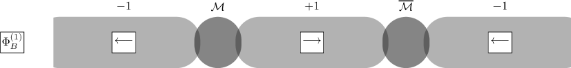
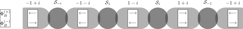
Figure 1: Sketch of monopole and semipole solutions on a straight string. At top is the situation when $m_{1}^{2}>m_{2}^{2}$, showing segments of string (light elongated shapes) with monopole ‘beads’ (dark circular shapes). The direction of the flux $\Phi_{B}^{(1)}$ (15) along the string segments is indicated by the direction of the arrows. At bottom, the case when $m_{1}^{2}=m_{2}^{2}$ and $\kappa>2\lambda$ is shown, with the dark circular shapes representing semipoles. Here, the arrows indicate the real and imaginary parts of the gauge invariant complex flux, Eq. (14). There are four possible string solutions labelled by $w$, with semipoles $\mathcal{S}$ interpolating between them where the subscripts give their complex flux. In the case where $\kappa<2\lambda$, the appearance is similar but with $\Phi_{B}^{(1,2)}$ replacing $\Phi_{B}^{(\pm)}$. Note that the arrangement of semipoles shown is unable to annihilate; other orderings would allow annihilation.

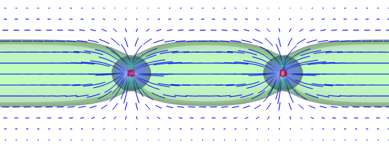
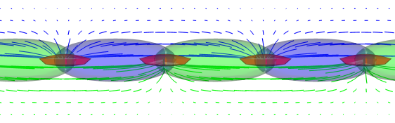
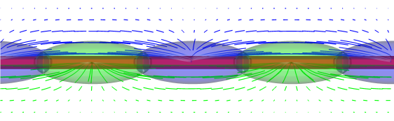
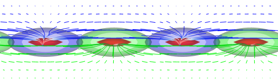
Figure 2: String segments from numerical solutions, showing isosurfaces of $\mathrm{Tr}\,\,\Phi_{1,2}^{2}=\frac{5}{16}v^{2}_{1,2}$ in blue and green respectively, and 90% isosurfaces of energy density in red. At the top, $(am_{1})^{2}=0.1$, $(am_{2})^{2}=0.04$ and $\kappa=1$. The $B^{(1)}$ field (8) is shown as blue streamlines on a vertical slice through the string, their length proportional to the field intensity at a given point. The other three images have $(am_{1})^{2}=(am_{2})^{2}=0.1$. Second to top is $\kappa=2$: Here, the $B^{(+)}$ and $B^{(-)}$ fields (9) are shown in blue and green, above and below the string (note that the streamlines are axially symmetric). The lower two images are of numerical solutions with $\kappa=1$ and $\kappa=0.5$, again showing $B^{(1)}$ streamlines in blue above the string, and the $B^{(2)}$ streamlines in green below.

Note that the strings carry half the flux of a monopole, and monopoles can therefore be thought of as threaded like a bead on a string Hindmarsh and Kibble (1985).

The theory of Eq. (1) has a number of global symmetries, which are important when enumerating the multiplicity of static solutions. Normally, we study the symmetries of the vacuum configuration, which has constant scalar field and zero gauge field strength, and we ignore transformations on the gauge field. However, we are also interested in the multiplicity of the vortex solutions, and so must be careful to include transformations on both scalar and gauge fields.

In the general case, the theory has a discrete global $Z_{2}\times Z_{2}$ symmetry $\Phi_{1}\to\pm\Phi_{1}$ and $\Phi_{2}\to\pm\Phi_{2}$, with the gauge field $A_{\mu}$ left alone. We note that it is always possible to find a gauge transformation which flips the signs of the scalar fields simultaneously: $\Phi_{n}\to-\Phi_{n}$. However, this gauge transformation will also change the gauge field. The difference between the global reflection and gauge transformations can be made explicit by considering the effective magnetic field operators

$$B^{(1)}_{i}={\rm Tr}\,B_{i}\hat{\Phi}_{1},~{}~{}B^{(2)}_{i}={\rm Tr}\,B_{i}\hat{\Phi}_{2},$$ (8)

where $\hat{\Phi}_{1,2}=\Phi_{1,2}/\sqrt{{\rm Tr}\,(\Phi_{1,2}^{2})}$ and $B_{i}=\frac{1}{2}\epsilon_{ijk}F^{jk}$. These are gauge invariant, but obviously change sign under the reflection of the scalar fields. These operators are used to quantify the magnetic flux in string solutions, along with a second set of gauge invariant magnetic fields

$$B^{(\pm)}_{i}={\rm Tr}\,B_{i}\hat{\Phi}_{\pm},$$ (9)

where

$$\hat{\Phi}_{\pm}=\frac{1}{\sqrt{2}}\left(\hat{\Phi}_{1}\pm\hat{\Phi}_{2}\right).$$ (10)

In the case of degenerate masses, $m_{1}^{2}=m_{2}^{2}=m^{2}$, the Lagrangian is invariant under interchange of the fields, $\Phi_{1}\leftrightarrow\Phi_{2}$, and so the discrete symmetry is enhanced. It can be seen that the sign change and interchange symmetries generate $D_{4}$, the group of symmetries of a square. Again, in a state with no gauge field strength (or $A_{\mu}\perp\Phi_{n}$), a sign change on the scalar fields is equivalent to a gauge transformation.

Given our specific form of potential (2), setting $\kappa=2\lambda$ means that the discrete symmetry is further enhanced to a global $\mathrm{O}(2)$ symmetry. This is most easily expressed in terms of a complexified $\mathrm{SU}(2)$ triplet $\Phi=(\Phi_{1}+i\Phi_{2})$ for which

$$V=m^{2}\,\mathrm{Tr}\,\Phi\Phi^{\dagger}+\frac{2\lambda-\kappa}{16}\left(\left(\mathrm{Tr}\,\Phi^{2}\right)^{2}+\left(\mathrm{Tr}\,\Phi^{{\dagger}\,2}\right)^{2}\right)\\ +\frac{\lambda}{2}\left(\mathrm{Tr}\,\Phi\Phi^{\dagger}\right)^{2}+\frac{2\lambda+\kappa}{8}\left(\mathrm{Tr}\,\Phi^{2}\right)\left(\mathrm{Tr}\,\Phi^{{\dagger}\,2}\right).$$ (11)

When $\kappa=2\lambda$ there are symmetry transformations

$$\Phi\to e^{i\alpha}\Phi\quad\text{and}\quad\Phi\to\Phi^{\dagger}$$ (12)

which are seen to generate the group $\mathrm{O}(2)$. The sign change $\Phi\to-\Phi$ is equivalent to a large gauge transformation on a state with no gauge field strength.

The global symmetries are not broken in the vacuum, as their transformations can be undone with a large gauge transformation. For example, choosing the gauge in which the vacuum is $(\Phi_{1},\Phi_{2})=(v_{1}\tau^{3},v_{2}\tau^{1})$, the effect of the change of sign of $\Phi_{1}$ can be undone with a gauge transformation $U=i\sigma^{1}$, while $U=i\sigma^{3}$ undoes the effect of a sign change on $\Phi_{2}$. In the degenerate case, the field interchange $\Phi_{1}\leftrightarrow\Phi_{2}$ can be undone with a gauge transformation $U=i(\sigma^{1}+\sigma^{3})/\sqrt{2}$.

However, some of the global symmetries are broken by the string solutions. We recall there are three cases: general, degenerate masses, and full global $\mathrm{O}(2)$ symmetry. In the first two cases there are two and four degenerate string solutions, separated by finite energy barriers. In the last case, there is a one-parameter family of string solutions.

To see that the string solution breaks the discrete symmetry in the general case, we use the magnetic field operator $B_{i}^{(1)}$, equation (8). It is clearly odd under the $Z_{2}$ symmetry $\Phi_{1}\to-\Phi_{1}$, and non-zero in the core of the string. Strings oriented in the $z$-direction can therefore be labelled by the sign of the magnetic flux $\Phi_{B}^{(1)}=\pm 2\pi/g$, with

$$\Phi_{B}^{(1,2)}=\int d^{2}x\,B^{(1,2)}_{i}\hat{z}_{i}.$$ (13)

In the mass degenerate case, we find three different types of string solutions depending on relative size of $\kappa$ and $2\lambda$. When $\kappa>2\lambda$, either $\Phi_{1}$ or $\Phi_{2}$ may vanish at the centre, meaning that there are two string solutions which, in a suitable gauge, may be written as (4–6) with $\Phi_{1}$ and $\Phi_{2}$ possibly interchanged. The orientation of the magnetic field along the string further divides the string solution to give four types.

In detail, we can use the magnetic field operators (9) to define a complex flux

$$\Phi_{B}=\Phi_{B}^{(+)}+i\Phi_{B}^{(-)}=w\frac{2\pi}{g}.$$ (14)

If $\Phi_{1}$ vanishes at the centre of the string, $\Phi_{B}^{(-)}=-\Phi_{B}^{(+)}=\pm 2\pi/g$, while if $\Phi_{2}$ vanishes at the centre of the string, $\Phi_{B}^{(-)}=\Phi_{B}^{(+)}=\pm 2\pi/g$. Hence $w=(\pm 1\pm i)$.

We see that string solutions are in one-to-one correspondence with the $Z_{2}\times Z_{2}$ group generated by sign changes of the fields. They leave unbroken a $Z_{2}$ subgroup of the original global symmetry $D_{4}$.

In the degenerate case with $\kappa<2\lambda$, it is energetically favourable for $\Phi_{1}$ and $\Phi_{2}$ to align or antialign in the core of the string, with either $\Phi_{B}^{(+)}$ or $\Phi_{B}^{(-)}$ vanishing. We can therefore label strings with the complex flux

$$\Phi^{\prime}_{B}=\Phi_{B}^{(1)}+i\Phi_{B}^{(2)}=w^{\prime}\frac{2\pi}{g}.$$ (15)

Again, $w^{\prime}=(\pm 1\pm i)$.

The string solutions are separated by finite-energy barriers, and so solutions can be constructed which interpolate between the string ground states as a function of $z$. We display sketches of these solutions in Fig. 1. In the general case, where there are two string ground states, the kink or antikink solutions interpolating between them are sources of flux which are the difference between the fluxes of the adjacent strings, or

$$\Phi_{B}^{(1)}=\pm 4\pi/g.$$ (16)

These beads can be interpreted as monopoles or antimonopoles trapped on the string, and like kinks correspond to an element of $Z_{2}$.

When $m_{1}^{2}=m_{2}^{2}$ and $\kappa>2\lambda$, the monopoles split into two “semipoles”, whose possible fluxes, again inferred from the differences between the fluxes of adjacent strings, are

$$\Phi_{B}=\{1,i,-1,-i\}4\pi/g.$$ (17)

Hence semipoles correspond to an element of $Z_{4}$. Two adjacent semipoles need not have total charge zero, and so need not annihilate. An equivalent argument applies to the charge $w^{\prime}$ in the case $\kappa<2\lambda$.

Finally, when the $D_{4}$ symmetry is enlarged to a $\mathrm{O}(2)$ symmetry (12) at $\kappa=2\lambda$ the monopoles become spread out, and there is instead a continuous phase at each point of the string, which is the argument of the complex parameter $w$ in Eq. (14) or $w^{\prime}$ in Eq. (15). In general, the phase can change along the string, giving rise to persistent currents, much like a superfluid.

These semipole and superfluid solutions are new, and were not anticipated in Ref. Hindmarsh and Kibble (1985).

We have performed the first 3-dimensional numerical simulations of the theory (1), in order to look for semipole solutions, and to investigate the dynamics of networks of necklaces in the early universe. We take $\lambda=1/2$ and $g=1$ so that the string tension is precisely $\pi v_{2}^{2}$ in the continuum. We perform simulations on $72^{3}$ periodic lattices with lattice spacing $a=1$, starting from random initial conditions. The system is evolved with heavy damping until it has relaxed to straight strings wrapping one of the directions in the simulation volume. Details, and numerical simulations of the string network, will be reported on in a separate publication Hindmarsh et al. (2016).

Fig. 2 shows isosurfaces of $\mathrm{Tr}\,\,\Phi_{1}^{2}$ (blue) and $\mathrm{Tr}\,\,\Phi_{2}^{2}$ (green) at $\frac{5}{16}v_{1,2}^{2}$, 90% isosurfaces of energy density (red), and streamlines of the vector fields $B_{i}^{(1)}$ (blue) and $B_{i}^{(2)}$ (green). In the general case, shown at the top with $(am_{1})^{2}=0.1$, $(am_{2})^{2}=0.04$ and $\kappa=2\lambda$, one expects to see strings as tubes of constant $\mathrm{Tr}\,\,\Phi_{2}^{2}$, with monopoles appearing as spheroids of constant $\mathrm{Tr}\,\,\Phi_{1}^{2}$. It is clear that this expectation is borne out.

We also show the three different degenerate cases – $\kappa=4\lambda$, $2\lambda$, $\lambda$, with $(am_{1})^{2}=(am_{2})^{2}=0.1$ – from second to top downwards in Fig. 2. In the $\kappa=4\lambda$ case (second to top) the blue and green streamlines are those of $B_{i}^{(+)}$ and $B_{i}^{(-)}$; otherwise they show $B_{i}^{(1)}$ and $B_{i}^{(2)}$.

One sees that the semipoles are sources of the magnetic fields $B_{i}^{(\pm)}$ ($\kappa>2\lambda$, second from top) or $B_{i}^{(1,2)}$ ($\kappa<2\lambda$, bottom), as explained above.

Finally, when $\kappa=2\lambda$, the accidental symmetry broken by the string is $\mathrm{O}(2)$, and there is a 1-parameter family of solutions labelled by the argument of $w$ (or equivalently $w^{\prime}$). Here, the energy density is uniform along the string.

In this paper we have found a new class of topological objects on strings in non-Abelian gauge theories, which we term semipoles. They are the result of the string breaking discrete symmetries of the Lagrangian, and can be viewed as half of a bead Hindmarsh and Kibble (1985). In the $\mathrm{SU}(2)$ theory we study they can be mapped to an element of $Z_{4}$.

The theory can be embedded in, for example, $\mathrm{SO}(10)$ with a Higgs in the 126 Kibble et al. (1982), where symmetry enforces the fields having the same mass scales and $\kappa=2\lambda$, and so models the string solution in an attractive class of Grand Unified Theories Jeannerot et al. (2003); Allys (2016a, b). Note that the complex flux we have used to classify the semipoles and strings cannot be defined in every case.

It is plausible that accidental global symmetries will be present in many GUT models, and that semipoles or superfluid degrees of freedom are generic features of high-scale cosmic strings. Such supercurrents might stabilise loops of string against collapse, resulting in an exotic form of metastable matter Copeland et al. (1987); Davis and Shellard (1989).

The cosmological implications of beads and semipoles depend on their average separation along the string $d$. It has been variously argued that $d$ evolves to the string width Berezinsky and Vilenkin (1997) or scales with the horizon Blanco-Pillado and Olum (2010). The latter argument assumed that the objects living on the string would annihilate if they encountered each other, which is not always the case with semipoles. The presence of massive objects on the strings affects the dynamics considerably Siemens et al. (2001). The uncertainty in theory, observational signals and constraints motivates the numerical investigation which we report on elsewhere Hindmarsh et al. (2016).