A Constrained Coding Scheme for Correcting Asymmetric Magnitude-$1$ Errors in $q$-ary Channels

Abstract

We present a constraint-coding scheme to correct asymmetric magnitude-$1$ errors in multi-level non-volatile memories. For large numbers of such errors, the scheme is shown to deliver better correction capability compared to known alternatives, while admitting low-complexity of decoding. Our results include an algebraic formulation of the constraint, necessary and sufficient conditions for correctability, a maximum-likelihood decoder running in complexity linear in the alphabet size, and upper bounds on the probability of failing to correct $t$ errors. Besides the superior rate-correction tradeoff, another advantage of this scheme over standard error-correcting codes is the flexibility to vary the code parameters without significant modifications.

I Introduction

The advent of multi-level non-volatile memories (NVMs) has introduced a plethora of coding problems on a variety of $q$-ary channels. Specifically, flash-memory based storage with multiple-level cells has become a fertile ground for addressing these coding problems. In the flash technology, a memory level is determined by the amount of electrical charge trapped inside a floating gate transistor. Equivalently, each memory level is represented by a certain value of voltage or current. However, due to a variety of factors such as noise, manufacturing variability, and inter-cell interference, it becomes very challenging to scale the number of levels while keeping the voltage dynamic range fixed. As a result, the gaps between memory levels become narrower, and a growing error rate compromises the data fidelity. Errors resulting from narrowing margins between levels have been an active subject of research in recent years. In particular, errors with asymmetry and magnitude limit have emerged as useful coding models to tackle this problem. Asymmetry of the errors stems from the inherent asymmetry between the write and erase operations in flash, which often renders one error direction much more dominant than the other. The limited magnitudes of the errors come from “incremental” error sources such as retention errors (slow decay of charge level) or disturbs (gradual level increments from writes to adjacent cells) [1],[2].

As the density scaling progresses, we expect that asymmetric, magnitude-$1$ errors will be the first to become the dominant reliability issue of multi-level NVMs. Hence our objective is to develop a coding scheme that will deal with a large number of asymmetric magnitude-$1$ errors within a code block. The coding scheme we propose herein will be evaluated in comparison to known coding techniques for asymmetric magnitude-$1$ errors, which we now briefly survey. In the extreme scenario, we can use an all asymmetric magnitude-$1$ error correcting code, which is equivalent to using only the even cell levels out of the $q$ supported levels [3]. A slightly less redundant code, correcting asymmetric magnitude-$1$ errors in up to half of the code coordinates, can be obtained by the construction of [4] when used with the binary repetition code. This option is equivalent to using only even levels or only odd levels within each codeword – hence termed even/odd in the sequel. When the code block length is not too large, we may also use the construction of [4] with lower-redundancy binary codes, such as BCH codes, to achieve a better tradeoff between rate and correctability. A generalization of [4], to more general error distributions can be found in [5]. Finally, another alternative is to use codes coming from the recently developed theory for L1 distance codes reported in a sequence of papers by Bose, Tallini and others. See for example [6] and citations thereof. In the sequel we show that for moderate to high error rates, our coding scheme gives a better correctability-rate tradeoff compared to the existing alternatives.

The proposed scheme, based on constraint coding, encodes data in a way that asymmetric magnitude-$1$ errors will be easily detected and corrected, but with milder restrictions than the all-errors correcting all-even code or the half-errors correcting even/odd code. The scheme is called Non-Consecutive Constraint (NCC), attesting to the enforced constraint of disallowing the codeword to contain two adjacent levels from $\{0,\ldots,q-1\}$. The NCC scheme has three main advantages:

1. Performance: the NCC outperforms alternative coding schemes for random errors, when the error rate is moderate to high.

2. Complexity: the decoder of the NCC has low complexity, and achieves the performance of the maximum likelihood (ML) decoder.

3. Flexibility: the tradeoff between the redundancy of the code and its error correction capabilities can be easily adjusted without re-designing the code or altering the decoder and encoder.

Section II describes common coding schemes for asymmetric errors, Section III presents the NCC coding scheme and its algebraic formulation. It is an important fact that the resilience of a codeword against asymmetric magnitude-1 errors depends only on its histogram (how many code-positions have each $q$-ary symbol), and thus the algebraic study of the code works in the domain of word histograms. A maximum-likelihood, low complexity decoding algorithm for the NCC is presented in Section IV, and detailed performance analysis appears in Section V. Finally, finite block-length analysis for the corresponding information-theoretic model – the $q$-ary Z-channel – is presented in Section VI, and showing the good performance of the proposed coding scheme.

II Asymmetric Errors with Magnitude 1

As described in the introduction, we assume throughout the paper that all errors are asymmetric with magnitude $1$, in the downward direction. Obviously, when restricting the error pattern to asymmetric errors with magnitude $1$, using standard symmetric-error $q$-ary error correcting codes is wasteful. A general recipe for converting a standard error-correcting code to a higher-rate version of the code designed for asymmetric errors with magnitude $1$ can be found in [4]. The idea behind [4] in a nutshell is that in order to protect an $n$-cell $q$-ary memory block from asymmetric errors with magnitude $1$, we can convert the $q$-ary symbol to its binary form, encode only the least significant bits (LSBs) with a standard binary error correcting code, and map back to the $q$-ary form. By using this method, it is possible to use well-known codes and achieve very high-rate coding schemes. When using this recipe with the binary repetition code we get a $q$-ary code where in each codeword either all levels are even or all are odd. This scheme allows the correction of $\left\lfloor\frac{n-1}{2}\right\rfloor$ asymmetric magnitude-$1$ errors. Later in the paper we refer to this coding scheme as the even/odd code.

Example 1

. The following $q=8$, $n=4$ words $(2,2,4,0)$ and $(1,7,3,1)$ are legitimate even/odd codewords. However, $(2,2,4,1)$ is not a legitimate codeword since it contains both odd and even values. Notice that if an asymmetric error with magnitude $1$ occurs in the first coordinate of the first codeword we get $(1,2,4,0)$. After reading such a word we can definitely deduce that an error occurred. There are three even values and a single odd value, therefore, by taking the majority it is clear that the error occurred in the first coordinate and the original codeword can be successfully restored.

Another simple coding scheme is the all-even code [3], which is obtained by using only the even levels from the alphabet, and which can correct $n$ asymmetric magnitude-$1$ errors.

III The Non-Consecutive Constraint (NCC)

We now present the Non-Consecutive Constraint (NCC) coding scheme, which is specifically designed to correct large numbers of asymmetric errors with magnitude $1$. Let the state of the memory cell be represented as a discrete cell level $c$, taken from the integer set $\{0,\ldots,q-1\}$.

Definition 2

. The $NCC(n,q)$ is a constraint in which every $n$-cell, $q$-level memory block does not contain cells with consecutive memory levels.

Example 3

. The following $q=8$, $n=8$ codeword $(2,5,7,0,2,0,4,4)$ is not an NCC codeword (because $4,5$ are consecutive levels and both appear in the codeword). In contrast, $(2,4,4,0,2,0,4,7)$ is an NCC codeword.

While the definition of the NCC is relatively simple, its error-correcting capabilities are not straightforward, since correctability depends on both the codeword and the error pattern.

Definition 4

. A Maximum-Likelihood Decoder for the NCC decodes a given word to an NCC codeword that requires minimal number of magnitude-$1$ upward corrections.

Example 5

. Let us take the following $q=8$, $n=10$ NCC codeword $(6,6,6,6,6,2,2,2,2,2)$. Let us assume two of the five $6$’s suffer an asymmetric magnitude-1 error, thus we get the received word of $(5,5,6,6,6,2,2,2,2,2)$. Due to the violation of the NCC, it is easy to notice that this word is erroneous, meaning that either two $6$’s have suffered an error and became $5$, or three $7$’s have suffered an error and became $6$. The first option requires fewer magnitude-$1$ upward corrections, therefore selected. In a similar way, we can correct any other combination of two asymmetric magnitude-$1$ errors. However, in the $n=4$ codeword $(6,6,2,2)$ even a single error cannot be corrected. If one of the $6$’s suffers an error, for example, the erroneous word is $(5,6,2,2)$. In this case the decoder cannot choose between two maximum likelihood NCC codewords $(6,6,2,2)$ and $(5,7,2,2)$, each requiring one magnitude-$1$ upward correction.

III-A Information rate

Definition 6

. The information rate ${\cal R}$ of a code for $n$-cell, $q$-level memory array is defined as

$${\cal R}=log_{q}(M)/n,$$

where $M$ is the number of legal combinations according to the code specification. ${\cal R}$ represents the number of information $q$-ary symbols stored per physical cell.

Theorem 7

. The information rate of the $NCC(n,q)$ is given by

$${\cal R}_{NCC}\left(n,q\right)=\frac{1}{n}\log_{q}\left[\sum_{k=1}^{\frac{q}{2}}k!\cdot S\left(n,k\right)\cdot\binom{q-k+1}{k}\right],$$ (1)

where $S(n,k)$ is the Stirling number of the second kind [8].

Proof.

The number of combinations to occupy $k$ non-consecutive levels out of $q$ levels is $\binom{q-k+1}{k}$ [8](Ch.13). By multiplying it by the number of surjections from $n$-cell set to $k$-level set we obtain the desired combinations count. The number of surjections from an $n$-set to a $k$-set equals $k!\cdot S\left(n,k\right)$ [9]. Summing all possible values of $k$ gives exactly the expression inside the $\log$ in (1).   

In order to compare between the NCC and the even/odd and all-even coding schemes, we now quote the information rates for the other methods. Due to the fact that for an even/odd codeword all $n$ cells are either all even or all odd, the number of possible combinations is given by $M=2\cdot(q/2)^{n}$, assuming even $q$. Therefore, the information rate of the $n$-cell, $q$-level even/odd code is given by

$${\cal R}_{even/odd}\left(n,q\right)=1-\frac{n-1}{n}\log_{q}2.$$ (2)

The all-even code has an information rate that is independent of $n$, and is equal to $1-log_{q}2$. As a result, unlike the NCC and even-odd codes above, it is not possible to change the rate-correction tradeoff of all-even by varying its block size. Fig. 1 presents a comparison between the information rates of the three coding schemes as a function of the codeword length $n$. It can be observed that the information rate of the NCC is higher than even/odd and all-even for all values of $n$. However, for higher values of $n$ the difference between the codes gets smaller. The rate hierarchy reflected in Fig. 1 is no coincidence: the three codes are related through the proper inclusion of their codewords: $\text{all-even}\left(n,q\right)\subset\text{even/odd}\left(n,q\right)\subset NCC\left(n,q\right)$.

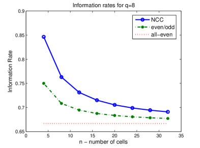
Figure 1: Information rates vs. number of cells per block for NCC (solid - circles) even/odd scheme (dash-dotted - stars) and all-even scheme (dotted)

Theorem 8

. When $n\rightarrow\infty$ and $q$ is fixed, the NCC, even/odd and all-even schemes have the same information rate.

The proof of Theorem 8 appears in Appendix A. Even though the NCC has the same rate as the even/odd and all-even schemes in the limit, we show in the sequel that for finite $n$ values it can give better rate/correction tradeoff.

III-B Algebraic formulation of the NCC

In order to better understand and analyze the NCC coding scheme, we turn to a more formal algebraic definition of the constraint. In the sequel, inequalities involving vectors are interpreted element-wise.

Definition 9

. Given a vector of cell levels $\boldsymbol{c}=(c_{1},\ldots,c_{n})$, with $c_{s}{\,\mathchar 12850\relax\,}\{0,\ldots,q-1\}$, define the histogram vector as the length-$q$ column vector $\boldsymbol{h}$ in which the $i$-th element $i{\,\mathchar 12850\relax\,}\{0,\ldots,q-1\}$ is the number of cells that occupy level $i$ in $\boldsymbol{c}$. That is, $h_{i}=\left|\left\{s{\,\mathchar 12850\relax\,}\{1,\ldots,n\}|c_{s}=i\right\}\right|$ .

Example 10

. For the following $q=8$, $n=8$ cell-level vector $\boldsymbol{c}=(2,2,4,5,2,2,4,0)$, we have $\boldsymbol{h}=[1,0,4,0,2,1,0,0]^{T}$.

In the remainder of the section we discuss only histogram vectors and not cell-level vectors, but keeping in mind that there is a many-to-one relation between cell-level vectors and histogram vectors.

Proposition 11

. Let $\boldsymbol{h}$ be a histogram vector of some memory word. $\boldsymbol{h}$ is a histogram of a legal NCC codeword if and only if it satisfies

$$diag\left(\boldsymbol{h}\right)A\boldsymbol{h}=\boldsymbol{0},$$ (3)

where $diag\left(\boldsymbol{h}\right)$ stands for a square diagonal matrix with the elements of vector $\boldsymbol{h}$ on its main diagonal,

$$A\triangleq\begin{pmatrix}0&1&0&\cdots&0\\ 0&0&1&\cdots&0\\ \vdots&\vdots&\vdots&\ddots&0\\ 0&0&0&\cdots&1\\ 0&0&0&0&0\end{pmatrix},$$ (4)

and $\boldsymbol{0}$ is the all-zero column vector.

Proof.

$A\boldsymbol{h}$ is the shifted histogram $[h_{1},h_{2},\ldots,h_{q-1},0]^{T}$, and $diag\left(\boldsymbol{h}\right)A\boldsymbol{h}$ is the scalar multiplication of the vectors $\boldsymbol{h}$ and $A\boldsymbol{h}$. Therefore, we get

$$diag\left(\boldsymbol{h}\right)A\boldsymbol{h}=\left[h_{0}\cdot h_{1},h_{1}\cdot h_{2},\ldots,h_{q-2}\cdot h_{q-1},0\right]^{T},$$ (5)

and requiring this vector to be the all-zero vector is equivalent to having no two consecutive occupied levels.   

Let $\boldsymbol{h}$ be a histogram vector of some memory word, and let $\boldsymbol{e}$ be an error histogram vector with all non-negative elements, whose $i$-th element specifies how many memory cells moved from level $i$ to level $i-1$ due to asymmetric magnitude-$1$ errors. The effect of each such error is decrementing $h_{i}$ and incrementing $h_{i-1}$. As a result, we get that the received histogram $\boldsymbol{w}$ is

$$\boldsymbol{w}=\boldsymbol{h}+T\boldsymbol{e},$$ (6)

where

$$T\triangleq\left(\begin{array}[]{rrrrrr}0&1&0&0&\cdots&0\\ 0&-1&1&0&\cdots&0\\ 0&0&-1&1&\cdots&0\\ \vdots&\vdots&\vdots&\ddots&\ddots&\vdots\\ 0&0&0&\cdots&-1&1\\ 0&0&0&0&\cdots&-1\\ \end{array}\right)_{q\times q}.$$ (7)

Note that by definition $\boldsymbol{e}$ should satisfy $\boldsymbol{e}\leqslant\boldsymbol{h}$. We now define the matrix

$$T^{{\dagger}}\triangleq\left(\begin{array}[]{rrrrrr}0&0&0&0&\cdots&0\\ 0&-1&-1&-1&\cdots&-1\\ 0&0&-1&-1&\cdots&-1\\ \vdots&\vdots&\vdots&\ddots&\ddots&\vdots\\ 0&0&0&\cdots&-1&-1\\ 0&0&0&0&\cdots&-1\\ \end{array}\right)_{q\times q},$$ (8)

and observe that it represents the inverse action of $T$ because $T^{{\dagger}}T$ gives the identity mapping on length $q$ vectors of the form $(0,u_{1},\ldots,u_{q-1})$, which is exactly the form of error histogram vectors $\boldsymbol{e}$.

Definition 12

. Given two histogram vectors $\boldsymbol{h_{1}},\boldsymbol{h_{2}}$ we define their downward difference vector $\boldsymbol{d}$ and their upward difference vector $\boldsymbol{\hat{d}}$ as follows

$$\boldsymbol{d}\left(\boldsymbol{h_{1}},\boldsymbol{h_{2}}\right)=\frac{T^{{\dagger}}\left(\boldsymbol{h_{2}}-\boldsymbol{h_{1}}\right)+|T^{{\dagger}}\left(\boldsymbol{h_{2}}-\boldsymbol{h_{1}}\right)|}{2},$$

$$\boldsymbol{\hat{d}}\left(\boldsymbol{h_{1}},\boldsymbol{h_{2}}\right)=-\frac{T^{{\dagger}}\left(\boldsymbol{h_{2}}-\boldsymbol{h_{1}}\right)-|T^{{\dagger}}\left(\boldsymbol{h_{2}}-\boldsymbol{h_{1}}\right)|}{2}.$$ (9)

$|\cdot|$ represents element-wise absolute value. Notice that the elements of $\boldsymbol{d}$ and $\boldsymbol{\hat{d}}$ are non-negative. In addition, $\boldsymbol{d}\left(\boldsymbol{h_{1}},\boldsymbol{h_{2}}\right)-\boldsymbol{\hat{d}}\left(\boldsymbol{h_{1}},\boldsymbol{h_{2}}\right)=T^{{\dagger}}\left(\boldsymbol{h_{2}}-\boldsymbol{h_{1}}\right)$. We now move to define a distance function for histograms. In all the discussion of the distance, we assume that the histogram vectors have the same length (the alphabet size $q$), and the same sum (the block size $n$).

Definition 13

. Given two histogram vectors $\boldsymbol{h_{1}},\boldsymbol{h_{2}}$ we define their downward distance ${\cal D}^{\downarrow}$ and their upward distance ${\cal D}^{\uparrow}$ as follows

$${\cal D}^{\downarrow}\left(\boldsymbol{h_{1}},\boldsymbol{h_{2}}\right)=\|\boldsymbol{d}\left(\boldsymbol{h_{1}},\boldsymbol{h_{2}}\right)\|,$$

$${\cal D}^{\uparrow}\left(\boldsymbol{h_{1}},\boldsymbol{h_{2}}\right)=\|\boldsymbol{{\hat{d}}}\left(\boldsymbol{h_{1}},\boldsymbol{h_{2}}\right)\|.$$ (10)

$\|\cdot\|$ stands for the $\ell_{1}$ vector norm.

Note the symmetry properties of the distance functions $\boldsymbol{d}\left(\boldsymbol{h_{2}},\boldsymbol{h_{1}}\right)=\boldsymbol{\hat{d}}\left(\boldsymbol{h_{1}},\boldsymbol{h_{2}}\right)$, and ${\cal D}^{\downarrow}\left(\boldsymbol{h_{2}},\boldsymbol{h_{1}}\right)={\cal D}^{\uparrow}\left(\boldsymbol{h_{1}},\boldsymbol{h_{2}}\right)$.

Example 14

. For the following $q=8$, $n=8$ histograms $\boldsymbol{h_{1}}=[0,2,0,3,3,0,0,0]^{T}$ and $\boldsymbol{h_{2}}=[2,0,0,2,4,0,0,0]^{T}$, the downward and upward difference vectors are $\boldsymbol{d}(\boldsymbol{h_{1}},\boldsymbol{h_{2}})=\left[0,2,0,0,0,0,0,0\right]^{T}$ and $\hat{\boldsymbol{d}}(\boldsymbol{h_{1}},\boldsymbol{h_{2}})=\left[0,0,0,0,1,0,0,0\right]^{T}$, respectively. The downward and upward distances are ${\cal D}^{\downarrow}(\boldsymbol{h_{1}},\boldsymbol{h_{2}})=2$ and ${\cal D}^{\uparrow}(\boldsymbol{h_{1}},\boldsymbol{h_{2}})=1$, respectively. In other words, in order to get $\boldsymbol{h_{2}}$ from $\boldsymbol{h_{1}}$, it is required to perform ${\cal D}^{\downarrow}(\boldsymbol{h_{1}},\boldsymbol{h_{2}})=2$ downward movements of elements in $\boldsymbol{h_{1}}$ (from level $2$ to $1$) and ${\cal D}^{\uparrow}(\boldsymbol{h_{1}},\boldsymbol{h_{2}})=1$ upward movement (from level $3$ to $4$).

A tool to analyze and design codes is the measure of $t$-confusability between histograms.

Definition 15

. The histogram $\boldsymbol{h_{1}}$ is $t$-confusable as $\boldsymbol{h_{2}}$ if after suffering $t$ errors (or less) a maximum-likelihood decoder returns $\boldsymbol{h_{2}}$.

Note that the definition of $t$-confusability does not mean that every pair of cell-level vectors with the corresponding histograms is $t$-confusable. But it does mean that there exists at least one such pair of cell-level vectors that can confuse the decoder in the case of $t$ errors or less.

Proposition 16

. $\boldsymbol{h_{1}}$ is $t$-confusable as $\boldsymbol{h_{2}}$ if and only if the following two conditions hold

1. $\boldsymbol{d}\left(\boldsymbol{h_{1}},\boldsymbol{h_{2}}\right)\leqslant\boldsymbol{h_{1}}$, $\boldsymbol{\hat{d}}\left(\boldsymbol{h_{1}},\boldsymbol{h_{2}}\right)\leqslant\boldsymbol{h_{2}}$,

2. ${\cal D}^{\uparrow}\left(\boldsymbol{h_{1}},\boldsymbol{h_{2}}\right)\leqslant{\cal D}^{\downarrow}\left(\boldsymbol{h_{1}},\boldsymbol{h_{2}}\right)\leqslant t$.

Proof.

If $\boldsymbol{h_{1}}$ can be confused as $\boldsymbol{h_{2}}$ after suffering $t$ errors, then there exist two error histogram vectors $\boldsymbol{e}\leqslant\boldsymbol{h_{1}}$ and $\boldsymbol{f}\leqslant\boldsymbol{h_{2}}$ such that $\|\boldsymbol{f}\|\leqslant\|\boldsymbol{e}\|\leqslant t$ that satisfy $\boldsymbol{h_{1}}+T\boldsymbol{e}=\boldsymbol{h_{2}}+T\boldsymbol{f}$. By reordering and multiplying by $T^{{\dagger}}$ we get that $T^{{\dagger}}\left(\boldsymbol{h_{2}}-\boldsymbol{h_{1}}\right)=\boldsymbol{e}-\boldsymbol{f}$. It follows from Definition 12 that $\boldsymbol{d}\left(\boldsymbol{h_{1}},\boldsymbol{h_{2}}\right)=\boldsymbol{e}-\boldsymbol{c}$, $\boldsymbol{\hat{d}}\left(\boldsymbol{h_{1}},\boldsymbol{h_{2}}\right)=\boldsymbol{f}-\boldsymbol{c}$ for some non-negative vector $\boldsymbol{c}$, and conditions 1 and 2 hold by the properties of $\boldsymbol{e},\boldsymbol{f}$.
For the other direction we assume that the conditions are met and examine the vectors $\boldsymbol{w}=\boldsymbol{h_{1}}+T\boldsymbol{d}\left(\boldsymbol{h_{1}},\boldsymbol{h_{2}}\right)$ and $\boldsymbol{w}^{\prime}=\boldsymbol{h_{2}}+T\boldsymbol{\hat{d}}\left(\boldsymbol{h_{1}},\boldsymbol{h_{2}}\right)$. By subtracting the equations and multiplying by $T^{{\dagger}}$ we get that $T^{{\dagger}}(\boldsymbol{w}^{\prime}-\boldsymbol{w})=\boldsymbol{0}$. We can conclude that $\boldsymbol{w}^{\prime}=\boldsymbol{w}$ because the only solutions to the linear system $T^{{\dagger}}\boldsymbol{x}=\boldsymbol{0}$ are of the form $[x_{0},0,\ldots,0]$, and necessarily $x_{0}=0$ because $\boldsymbol{w}$ and $\boldsymbol{w^{\prime}}$ sum to the same value $n$. Hence the received histogram $\boldsymbol{w}=\boldsymbol{w^{\prime}}$ will confuse the decoder when $\boldsymbol{h_{1}}$ is stored and the error is $\boldsymbol{d}\left(\boldsymbol{h_{1}},\boldsymbol{h_{2}}\right)$.   

The following proposition specializes the $t$-confusability conditions to the case where the histograms are NCC histograms.

Proposition 17

. Let $\boldsymbol{h}$ and $\boldsymbol{g}$ be NCC histograms, and denote $\boldsymbol{e}=\boldsymbol{d}\left(\boldsymbol{h},\boldsymbol{g}\right)$, $\boldsymbol{f}=\boldsymbol{\hat{d}}\left(\boldsymbol{h},\boldsymbol{g}\right)$. If $\boldsymbol{h}$ is $t$-confusable as $\boldsymbol{g}$ then for every $i$

$$h_{i}\cdot\left[\left(e_{i}-e_{i-1}\right)-\left(f_{i}-f_{i-1}\right)\right]+h_{i-1}\cdot\left[\left(e_{i+1}-e_{i}\right)-\left(f_{i+1}-f_{i}\right)\right]+$$

$$\left[\left(e_{i}-e_{i-1}\right)-\left(f_{i}-f_{i-1}\right)\right]\cdot\left[\left(e_{i+1}-e_{i}\right)-\left(f_{i+1}-f_{i}\right)\right]=0,$$ (11)

where $h_{i},e_{i},f_{i}$ are the $i$-th elements of the histogram vectors $\boldsymbol{h},\boldsymbol{e},\boldsymbol{f}$, respectively.

Proof.

Given that $\boldsymbol{h}$ and $\boldsymbol{g}$ satisfy the two conditions of Proposition 16, it is clear that $\boldsymbol{h}+T\boldsymbol{e}=\boldsymbol{g}+T\boldsymbol{f}$. In addition, given that $\boldsymbol{g}$ is also a histogram of an NCC codeword, it must also fulfill Proposition 11, giving

$$diag\left(\boldsymbol{h}+T\left(\boldsymbol{e}-\boldsymbol{f}\right)\right)A\left(\boldsymbol{h}+T\left(\boldsymbol{e}-\boldsymbol{f}\right)\right)=\boldsymbol{0}.$$ (12)

Solving (12) element-wise gives the expression in (11).   

The following proposition shows how the algebraic framework can be applied to prove correctability results.

Proposition 18

. Let $h_{i}$ be the $i$-th element of an NCC histogram $\boldsymbol{h}$. If $h_{i}>2t$ for each occupied level $i$, then $\boldsymbol{h}$ is not $t$-confusable as any NCC histogram.

Proof.

Let us assume that $\boldsymbol{h}$ is $t$-confusable as some other NCC histogram $\boldsymbol{g}$. Then by Proposition 17 the equation (11) is satisfied for every $i$. Recall that $\boldsymbol{e}=\boldsymbol{d}\left(\boldsymbol{h},\boldsymbol{g}\right)$ and $\boldsymbol{f}=\boldsymbol{\hat{d}}\left(\boldsymbol{h},\boldsymbol{g}\right)$; we now show that (11) cannot be satisfied under the conditions of this proposition. There exists a level $i$ with $e_{i}>0$, and by condition 1 in Proposition 16 we also get that $h_{i}>0$. By the NCC property, $h_{i-1}=0$ and $h_{i+1}=0$, which imply $e_{i-1}=e_{i+1}=0$. In addition, by the same NCC property on $\boldsymbol{g}$, either $f_{i-1}=f_{i+1}=0$ or $f_{i}=0$ (or both). Therefore, assigning these values in (11) gives two sets of equations

$$h_{i}\cdot\left(e_{i}-f_{i}\right)=\left(e_{i}-f_{i}\right)\cdot\left(e_{i}-f_{i}\right)$$ (13)

when $f_{i-1}=f_{i+1}=0$, or

$$h_{i}\cdot\left(e_{i}+f_{i-1}\right)=\left(e_{i}+f_{i-1}\right)\cdot\left(e_{i}+f_{i+1}\right)\Rightarrow$$

$$h_{i}=e_{i}+f_{i+1}$$ (14)

when $f_{i}=0$. Note that the two equations become the same if both $f_{i-1}=f_{i+1}=0$ and $f_{i}=0$. Given that $\boldsymbol{e}\neq\boldsymbol{f}$, there exists at least one $i$ for which  (13) implies $h_{i}=e_{i}-f_{i}$, a contradiction because $h_{i}>2t$. In addition, we have $\|\boldsymbol{f}\|\leqslant\|\boldsymbol{e}\|\leqslant t$ which implies that $f_{i+1}\leqslant t$, $e_{i}\leqslant t$, therefore, (14) cannot be satisfied as well. Hence we proved a contradiction showing that $\boldsymbol{h}$ has no $t$-confusable histograms.   

Remark: Proposition 18 can be further refined for the special case in which $h_{i}=2t$. In order to fulfill (14), we must have $e_{i}=f_{i+1}=t$. That means all $t$ errors occurred in level $i$ and a $t$-confusable histogram can only be created by moving the occupation of level $i$ to level $i+1$. This scenario can hold if and only if $h_{i-2}=h_{i+2}=0$.

Example 19

. Let us calculate the histogram patterns that are $1$-confusable as some other histograms, by using Proposition 17. Let us assume an error occurs in level $j$, hence $e_{j}=1$ and all the other values of $\boldsymbol{e}$ are $0$. We wish to find all possible values of $\boldsymbol{h}$ that are $1$-confusable as some other NCC histogram. When $e_{j}=1$ we know that $f_{j}=0$ (the error in the confusing histogram must be elsewhere), and using (14) we get three possible solutions

1. $h_{j}=2$, $f_{j+1}=1$ (by (14) with $i=j$). Then from the fact that $f_{i}=0$ for $i\neq j+1$ (a single error), we also get $h_{j-2}=0$ (by (11) with $i=j-1$), and $h_{j+2}=0$ (by (11) with $i=j+2$).

2. $h_{j}=1$, $f_{j+1}=0$ (by (14) with $i=j$), and $h_{j-2}=1$ (by (11) with $i=j-1$ and $f_{j-1}=1$).

3. $h_{j}=1$, $f_{j+1}=0$ (by (14) with $i=j$), and $h_{j-2}=0$ (by (11) with $i=j-1$ and $f_{j-1}=0$).

The solutions are graphically depicted in Fig 2. Pattern A in Fig 2 corresponds to the first solution, pattern B to the second one, and pattern C to the third solution.

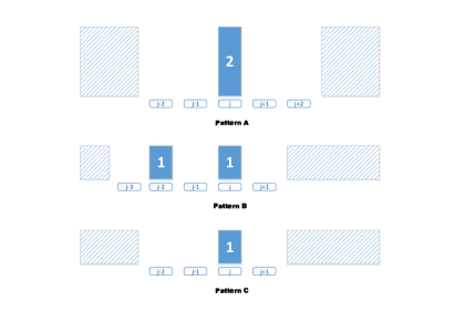
Figure 2: NCC histogram patterns that are 1-confusable as another NCC histogram. These histograms have at least one uncorrectable single error. Dashed bars represent don’t-care assignment.

IV Decoding & Encoding Algorithms for the NCC

IV-A A Decoding Algorithm

In this subsection we describe a decoding algorithm for the NCC. The objective is a maximum-likelihood decoding algorithm that finds the nearest codeword to the received memory word, in the sense that a minimal number of $+1$ cell transitions map between the memory word and the output codeword. The strengths of the proposed decoding algorithm are that it guarantees to return the nearest codeword, is invariant to the code block length $n$, and has very low complexity of ${\cal O}\left(q\right)$. To present the algorithm, we first give several formal definitions.

Definition 20

. For a histogram vector $\boldsymbol{h}$, we define a section ${\cal S}\left(\boldsymbol{h}\right)$ as a minimal-length sub-vector of $\boldsymbol{h}$ that is separated from other occupied levels by at least two empty levels. $N_{{\cal S}}\left(\boldsymbol{h}\right)$ is the number of sections in $\boldsymbol{h}$.

In the sequel, sections will be used by the algorithm as parts of the histogram that can be decoded independently.

Definition 21

. A burst $b\left(\boldsymbol{h}\right)$ is defined as a maximal length sub-vector in a histogram $\boldsymbol{h}$ with all its entries greater than zero. $N_{b}\left(\boldsymbol{h}\right)$ is the number of bursts in $\boldsymbol{h}$.

${\cal S}_{l}\left(\boldsymbol{h}\right)$ represents the $l$-th section of a certain histogram vector $\boldsymbol{h}$. We drop the $\boldsymbol{h}$ notation when it is clear to which histogram vector the section refers to. $b_{j}\left({\cal S}_{l}\right)$ represents the $j$-th burst in section ${\cal S}_{l}$, and for simplicity of notation, we denote $b_{j}\left({\cal S}_{l}\right)\equiv b_{j}^{l}$.

Example 22

. For the following $q=12$, $n=15$ histogram vector $\boldsymbol{h}=\left[2,0,0,1,3,1,0,0,1,2,0,5\right]^{T}$, there are three sections: ${\cal S}_{1}\left(\boldsymbol{h}\right)=\left[2\right]$, ${\cal S}_{2}\left(\boldsymbol{h}\right)=\left[1,3,1\right]^{T}$ and ${\cal S}_{3}\left(\boldsymbol{h}\right)=\left[1,2,0,5\right]^{T}$. The sections ${\cal S}_{1}$ and ${\cal S}_{2}$ contain only one burst each, and ${\cal S}_{3}$ has two bursts: $b_{1}^{3}=b_{1}\left({\cal S}_{3}\right)=\left[1,2\right]^{T}$ and $b_{2}^{3}=b_{2}\left({\cal S}_{3}\right)=\left[5\right]$.

From Definition 21, it is obvious that any burst of two levels or more must violate the NCC. Therefore, the purpose of the decoding algorithm is to resolve all the NCC violations expressed as a set of bursts. As a consequence, a decoded codeword must not contain a burst of two levels or more. An NCC violation in a burst can be resolved by up to two options: either all the burst occupations of odd levels must be moved up by one to the even ones, or all the burst occupations of even levels must be moved up to the odd ones (a graphic illustration is presented in Fig. 3). As will be explained further on, for some scenarios, only one of the movement options is possible.

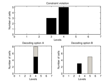
Figure 3: Constraint violation and two options for decoding: moving up the even level or moving up the odd level. Corrected cells are in gray.

Definition 23

. We define the movement that resolves the NCC violation induced by burst $b$ as either $\sigma\left(b\right)$, when keeping the highest level of $b$ intact, or $\bar{\sigma}\left(b\right)$, when the occupation of the highest level of $b$ is moved up.

Definition 24

. For a movement of levels $\pi(b)$, the cost of this movement ${\cal C}\left(\pi(b)\right)$ is defined as the number of cells whose level is moved in this action. When $\pi(b)$ includes the movement of cells occupying the level $q-1$ (which is impossible), we define ${\cal C}\left(\pi(b)\right)=\infty$.

During the decoding process, the different combinations for resolving bursts are determined in order to achieve minimal cost, hence, finding the nearest NCC codeword.

Example 25

. For $q=10$, $n=12$, let us assume we read a word with the histogram $\boldsymbol{h}=\left[0,4,2,0,0,1,0,0,3,2\right]^{T}$. From the existence of two-level bursts, it is clear that this memory word is corrupt by some errors. All three sections contain only one burst each; the burst of the first section is $b_{1}^{1}=\left[4,2\right]^{T}$. So in order to resolve this violation, it is possible to perform a $\bar{\sigma}\left(b_{1}^{1}\right)$ movement (which means we move the $2$ cells at level $2$ upward) and obtain $\left[4,0,2\right]^{T}$. Alternatively, we can perform a $\sigma\left(b_{1}^{1}\right)$ movement (moving the $4$ cells at level $1$ upward), and obtain $\left[0,6,0\right]^{T}$. The costs of these two movement options are $2$ and $4$, respectively, so in order to minimize the cost, it is obvious that $\bar{\sigma}\left(b_{1}^{1}\right)$ is preferred. The burst of the second section is $b_{1}^{2}=\left[1\right]$. In case this cell endured an error, it cannot be decoded successfully. The burst of the last section $b_{1}^{3}=\left[3,2\right]^{T}$ has only one correction option $\sigma\left(b_{1}^{3}\right)$, because level $q-1$ cannot move upward. The decoded histogram is therefore $\boldsymbol{h^{\prime}}=\left[0,4,0,2,0,1,0,0,0,5\right]^{T}$.

The decoding processes can work on each section independently, but multiple bursts within a section need to be decoded jointly. The decoder is thus specified below through the main iteration on sections in Algorithm 1, and with the decoding of an individual section as a dynamic-programming (Viterbi-like) subroutine in Algorithm 2.

input : $\boldsymbol{h}$

output : $\boldsymbol{h^{\prime}}$

for $l=1$ to $N_{{\cal S}}\left(\boldsymbol{h}\right)$

  $actionVec=$DecodeSection(${\cal S}_{l}\left(\boldsymbol{h}\right)$)

  correct $\boldsymbol{h}\Rightarrow\boldsymbol{h^{\prime}}$ by applying $actionVec$ on all $b_{j}{\,\mathchar 12850\relax\,}{\cal S}_{l}\left(\boldsymbol{h}\right)$

end

Algorithm 1 DecodeHistogram

The algorithm starts with the burst, and for every burst $j$ and a movement $\pi{\,\mathchar 12850\relax\,}\left\{\sigma,\bar{\sigma}\right\}$, it builds a concatenated cost table ${\cal W}_{j}\left(\pi\right)$, which holds the minimal cost of movements for resolving all bursts up to burst $j$. The algorithm also stores the movement path $\Pi_{j}$ which holds the sequence of movements with the optimal cost. During the burst iteration we distinguish between two cases: in a burst $j$ with odd length, not moving the high level of the burst necessitates not moving the high level of burst $j-1$, and in a burst $j$ with even length, moving the high level of burst $j$ necessitates not moving the high level of burst $j-1$. The decoding process ends with the highest burst that determines which movement is possible for the previous burst (which was already solved). It is clear that the decoding algorithm has ${\cal O}\left(q\right)$ complexity and uses two tables of size $2\sum_{l=1}^{N_{{\cal S}}}N_{b}\left({\cal S}_{l}\right)$, which is smaller than $2q$.

input : ${\cal S}$

output : $actionVec$

//initialization:

${\cal W}_{1}\left(\sigma\right)={\cal C}\left(\sigma\left(b_{1}\right)\right)$, ${\cal W}_{1}\left(\bar{\sigma}\right)={\cal C}\left(\bar{\sigma}\left(b_{1}\right)\right)$

$\Pi_{1}\left(\sigma\right)=\Pi_{1}\left(\bar{\sigma}\right)=\emptyset$

//tables fill

for $j=2$ to $N_{b}\left({\cal S}\right)$

  $\alpha=argmin_{\left\{\sigma,\bar{\sigma}\right\}}\left({\cal W}_{j-1}\left(\sigma\right),{\cal W}_{j-1}\left(\bar{\sigma}\right)\right)$

//for odd-length bursts:

  ${\cal W}_{j}\left(\sigma\right)={\cal C}\left(\sigma\left(b_{j}\right)\right)+{\cal W}_{j-1}\left(\sigma\right)$

  $\Pi_{j}\left(\sigma\right)=\left[\Pi_{j-1}\left(\sigma\right),\sigma\right]$

  ${\cal W}_{j}\left(\bar{\sigma}\right)={\cal C}\left(\bar{\sigma}\left(b_{j}\right)\right)+\min\left({\cal W}_{j-1}\left(\sigma\right),{\cal W}_{j-1}\left(\bar{\sigma}\right)\right)$

  $\Pi_{j}\left(\bar{\sigma}\right)=\left[\Pi_{j-1}\left(\alpha\right),\alpha\right]$

//for even-length bursts:

  ${\cal W}_{j}\left(\sigma\right)={\cal C}\left(\sigma\left(b_{j}\right)\right)+\min\left({\cal W}_{j-1}\left(\sigma\right),{\cal W}_{j-1}\left(\bar{\sigma}\right)\right)$

  $\Pi_{j}\left(\sigma\right)=\left[\Pi_{j-1}\left(\alpha\right),\alpha\right]$

  ${\cal W}_{j}\left(\bar{\sigma}\right)={\cal C}\left(\bar{\sigma}\left(b_{j}\right)\right)+{\cal W}_{j-1}\left(\sigma\right)$

  $\Pi_{j}\left(\bar{\sigma}\right)=\left[\Pi_{j-1}\left(\sigma\right),\sigma\right]$

end

//making final decision

$\alpha=argmin_{\left\{\sigma,\bar{\sigma}\right\}}\left({\cal W}_{N_{b}\left({\cal S}\right)}\left(\sigma\right),{\cal W}_{N_{b}\left({\cal S}\right)}\left(\bar{\sigma}\right)\right)$

$actionVec=\left[\Pi_{N_{b}}\left(\alpha\right),\alpha\right]$

Algorithm 2 DecodeSection

IV-B An Encoding Algorithm

In this section we present an encoder for the NCC. The purpose of the encoder is to map a decimal value $x$ to an $n$-cell, $q$-level NCC codeword. The main idea behind the encoder is translating the analytic expression counting NCC codewords (1) to a constructive mapping. We start with the following definitions.

Definition 26

. Let $LUT$ be a look-up table whose $q/2$ elements are calculated by

$$LUT\left(k\right)=\sum_{i=1}^{k}i!\cdot S\left(n,i\right)\cdot\binom{q-i+1}{i},$$ (15)

where $1\leqslant k\leqslant\frac{q}{2}$.

Definition 27

. Let $\lambda\left(m,k,j\right)$ be an enumeration function mapping an integer $j$ out of $1,\ldots,\binom{m}{k}$ to a subset of $k$ distinct indices from $\{0,\ldots,m-1\}$.

Example 28

. For $m=4$ and $k=2$, the value of $j$ is between $1$ to $\binom{4}{2}=6$, and corresponds to one of the following sets: $\left\{1,2\right\},\left\{1,3\right\},\left\{1,4\right\},\left\{2,3\right\},\left\{2,4\right\},\left\{3,4\right\}$. Therefore, e.g. $\lambda\left(4,2,1\right)=\left\{1,2\right\}$ and $\lambda\left(4,2,6\right)=\left\{3,4\right\}$.

Definition 29

. Let $\pi\left(k,i\right)$ be an enumeration function mapping an integer $i$ in the interval $1,\ldots,k!$ to a permutation of the indices $1,\ldots,k$.

Algorithm 3 presents a recursive ${\cal O}\left(n\right)$ algorithm that enumerates partitions counted by the Stirling numbers of the second kind, and maps integers to partitions.

input : $n,k,x$

output : ${\cal P}$

//recursion termination conditions

if $n=k$

  ${\cal P}=\left[\left\{c_{1}\right\},\left\{c_{2}\right\},\ldots,\left\{c_{n}\right\}\right]$

elseif $k=1$

  ${\cal P}=\left[\left\{c_{1},c_{2},\ldots,c_{n}\right\}\right]$

end

//following Stirling’s recurrence

$\tilde{x}=x-k\cdot S\left(n-1,k\right)$

if $\tilde{x}>0$

  $\tilde{{\cal P}}=StirPar\left(n-1,k-1,\tilde{x}\right)$

  ${\cal P}=\left[\left\{c_{n}\right\},\tilde{{\cal P}}\right]$

else

  $\tilde{k}=\left\lceil x/S\left(n-1,k\right)\right\rceil$

  $\tilde{x}=x-\left(\tilde{k}-1\right)\cdot S\left(n-1,k\right)$

  $\tilde{{\cal P}}=StirPar\left(n-1,k,\tilde{x}\right)$

  append $c_{n}$ to $\tilde{k}-th$ element of $\tilde{{\cal P}}$ and return as ${\cal P}$

end

Algorithm 3 StirPar

Example 30

. There are $S\left(5,3\right)=25$ partitions of an $n=5$ set to $k=2$ non-empty sets. Using Algorithm 3 gives $StirPar\left(5,3,4\right)=\left\{c_{4},c_{5}\right\},\left\{c_{3},c_{1}\right\},\left\{c_{2}\right\}$, and $StirPar\left(5,3,23\right)=\left\{c_{5}\right\},\left\{c_{1}\right\},\left\{c_{2},c_{3},c_{4}\right\}$.

We now present the encoding process of $x$ to a length-$n$ NCC codeword by the following steps. Encoding starts with the following calculations:

1. Let $k$ be the minimal index of LUT for which $x<LUT\left(k\right)$. $k$ represents the number of occupied levels in the histogram of the encoded codeword. If $k>1$ set $y=x-LUT\left(k-1\right)$, otherwise set $y=x$.

2. Let $i_{\pi}=\left\lfloor y/\left(S\left(n,k\right)\binom{q-k+1}{k}\right)\right\rfloor+1$

3. Let $j_{\lambda}=\left\lfloor\left(y-\left(i_{\pi}-1\right)S\left(n,k\right)\binom{q-k+1}{k}\right)/S\left(n,k\right)\right\rfloor+1$

4. Let $\hat{y}=y-\left(i_{\pi}-1\right)S\left(n,k\right)\binom{q-k+1}{k}-\left(j_{\lambda}-1\right)S\left(n,k\right)+1$

After calculating $k,i_{\pi},j_{\lambda},\hat{y}$ we can now construct the NCC codeword by the following steps.

1. Let $\boldsymbol{s}$ be the length-$k$ vector whose elements are the $k$ elements of $\lambda\left(q-k+1,k,j_{\lambda}\right)$ in ascending order.

2. To each index $i=1,\ldots,k$ in $\boldsymbol{s}$, add the value $i-1$.

3. Let ${\cal P}$ be a partition obtained by $StirPar\left(n,k,\hat{y}\right)$.

4. Permute ${\cal P}$ by the permutation obtained by $\pi\left(k,i_{\pi}\right)$.

5. Create the NCC codeword by assigning the cells that appear in the $i$-th set of ${\cal P}$ to the level equaling the $i$-th element of $\boldsymbol{s}$.

Example 31

. Let us assume we wish to encode the value $x=1660$ to an $n=5$, $q=8$ NCC codeword. We start with the preliminary calculations that give:

1. $LUT=\left[8,638,3638,4838\right]$ therefore $k=3$, we set $y=1660-638=1022$

2. $i_{\pi}=3$

3. $j_{\lambda}=1$

4. $\hat{y}=23$

We now construct the codeword by:

1. $\boldsymbol{s}=\lambda\left(6,3,1\right)=\left[0,1,2\right]$.

2. After applying the second step we get $\boldsymbol{s}=\left[0,2,4\right]$.

3. ${\cal P}=StirPar\left(5,3,23\right)=\left\{c_{5}\right\}\left\{c_{1}\right\}\left\{c_{2},c_{3},c_{4}\right\}$.

4. $\pi\left(3,3\right)=\left(3,2,1\right)$, so after permuting ${\cal P}$ we get ${\cal P}=\left\{c_{2},c_{3},c_{4}\right\}\left\{c_{1}\right\}\left\{c_{5}\right\}$.

5. By pairing ${\cal P}$ with $\boldsymbol{s}$ we get the following codeword $\boldsymbol{c}=\left(2,0,0,0,4\right)$.

So the decimal value $x=1660$ is encoded to the $n=5$, $q=8$ NCC codeword $\boldsymbol{c}=\left(2,0,0,0,4\right)$.

The reverse mapping is a straightforward application of the same steps above in reverse order.

V Performance Analysis

In this section we wish to evaluate the error-correcting performance of the NCC code. An exact calculation of the correction probability is challenging in general, so we derive lower bounds. We also show experimentally that the NCC code gives superior performance to known coding alternatives for the same error model.

V-A Experimental results

Table I presents the correction performance of the NCC code for $q=8$. The two left columns include the code length $n$ and its corresponding information rate. The rest of the table presents the probability to fully-correct a specified number of uniformly distributed asymmetric magnitude-$1$ errors.

TABLE I: Full-correction probability for the $n$-cell 8-level NCC

$q=8$		Total number of errors $\left\|\boldsymbol{e}\right\|$
n	${\cal R}_{NCC}$	1	2	3	4	5	6
5	0.816	0.801	0.478	0.170	0.043	0.007	0
9	0.752	0.967	0.908	0.805	0.635	0.384	0.193
13	0.726	0.993	0.981	0.960	0.927	0.869	0.777
17	0.712	0.998	0.995	0.990	0.983	0.971	0.952

As can be seen in Table I, the correction capability improves as $n$ increases (but the rate decreases). Moving between rows in the table to different rate-correction tradeoffs is done flexibly without need to change the decoder. Note that there is no guarantee that given a certain number of errors it can always be fully corrected. Whether a certain error can be corrected depends on both the codeword and the error pattern. What does not show in the table is that even in instances that did not fully correct, many of the errors were indeed corrected. In fact, this property will be next shown to result in superior performance of NCC. The way we compare the codes’ performance is by measuring the symbol-error rate (SER) at the decoder output for a given rate of asymmetric magnitude-$1$ errors at the input. In Fig. 4 we plot the output SER for three codes: even/odd, $BCH\left(15,5,7\right)$ and length $7$ NCC, with equal rate of $0.777$ (plus a no-coding option). The quoted BCH code is a binary code that is used in the construction of [4] to get asymmetric magnitude-$1$ correction. The x-axis is the input SER, which is the probability that a symbol exhibits an asymmetric magnitude-$1$ error.

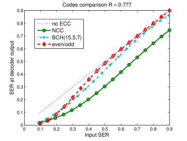
Figure 4: Correcting capabilities as a function of media SER for information rate of 0.777 and $q=8$. NCC (solid & circles), BCH(15,5,7) (dashed & diamonds), even-odd (semi-dashed & pluses). Rate 1 no-ECC option is shown as reference (dotted).

From Fig. 4 one can notice that the NCC code outperforms all the other codes with equal rate, for input SER values around 0.2 and higher. The SER remaining at the decoder output will be taken care of by a standard ECC, which in the case of NCC will require less redundancy because of the lower residual error rates. Note that the short lengths of the NCC code blocks do not limit the size of the memory word lines. Long word-lines can be supported by concatenating multiple NCC codewords.

V-B Bounds on performance

In this sub-section, we study analytically the decoding performance of the NCC code. Here the objective is to analyze the block-error performance of the code, that is, its ability to correct all the errors that corrupted the codeword. Given $t$, we are interested in the probability ${\cal P}_{t}$ that the ML decoder fails to correct all $t$ errors, where the probability is calculated with the uniform distribution on both the error locations and the stored codeword. Calculating this probability exactly seems a hard combinatorial problem, so we derive two upper bounds on ${\cal P}_{t}$. The first upper bound (Theorem 33) is simpler, albeit less tight. It also enables deriving the asymptotic behavior of the performance more easily. The second upper bound (Theorem 38) is a much tighter bound, but more complicated to derive and analyze. Let us first make the following definition.

Definition 32

. Let $B_{t}$ be a subset of the NCC code, $B_{t}\subset NCC(n,q)$, which includes all the codewords whose histogram vector $\boldsymbol{h}$ satisfy $h_{i}>2t,\;\forall i:\;h_{i}\neq 0$.

By Proposition 18, it is clear that for every codeword in $B_{t}$ enduring $t$ errors, it is guaranteed that all $t$ errors can be corrected.

Theorem 33

. Given that $t\leqslant\left\lfloor\frac{n}{5}\right\rfloor+1$ uniformly selected errors occurred in a uniformly selected $NCC(n,q)$ codeword, the ML decoding-failure probability ${\cal P}_{t}$ is bounded from above by

$${\cal P}_{t}\leqslant\frac{\sum_{k=1}^{q/2}k!F_{2t+1}\left(n,k\right)\cdot\left[\binom{q-k+1}{k}-1\right]\cdot\frac{2kt}{n}}{M},$$ (16)

where $M=q^{n{\cal R}_{NCC}\left(n,q\right)}$ is the number of $n$-cell, $q$-level NCC codewords, and

$$F_{r}\left(n,k\right)\triangleq S\left(n,k\right)-S_{r}\left(n,k\right),$$ (17)

where $S_{r}(n,k)$ are the $r$-associated Stirling numbers of the second kind [10]. (The combinatorial interpretation of $S_{r}(n,k)$ is the number of partitions of an $n$-set to $k$ subsets, all of which are of cardinality at least $r$.)

Proof.

Let us consider the subset $B_{t}$ from Definition 32. By Proposition 18, it is clear that for every codeword $\boldsymbol{c}{\,\mathchar 12850\relax\,}NCC(n,q)$

$$Prob\left(failure\,|\,\boldsymbol{c}{\,\mathchar 12850\relax\,}B_{t}\right)=0,$$

$$Prob\left(failure\,|\,\boldsymbol{c}{\,\mathchar 12850\relax\,}\bar{B}_{t}\right)\geqslant 0,$$ (18)

where $\bar{B}_{t}$ is the codeword subset complementary to $B_{t}$. For the bound we need to analyze the dependence of decoding failure on the error pattern, in addition to its dependence on $\boldsymbol{c}$. For a given codeword in $\bar{B}_{t}$, some error patterns cause a decoding failure while others do not. Let us define $E\left(\boldsymbol{c}\right)$ as the set of all the error patterns $\boldsymbol{e}$ which make the decoder fail on codeword $\boldsymbol{c}$. Therefore, the total decoding-failure probability is given by

$$Prob\left(failure\right)=Prob\left(\boldsymbol{c}{\,\mathchar 12850\relax\,}\bar{B}_{t}\right)\cdot Prob\left(\boldsymbol{e}{\,\mathchar 12850\relax\,}E\left(\boldsymbol{c}\right)|\boldsymbol{c}{\,\mathchar 12850\relax\,}\bar{B}_{t}\right).$$ (19)

We first calculate an upper bound on $Prob\left(\boldsymbol{c}{\,\mathchar 12850\relax\,}\bar{B}_{t}\right)$ by calculating an upper bound on the size of the subset $\bar{B}_{t}$. The definition of $B_{t}$ implies that each codeword in $\bar{B}_{t}$ contains at least one memory level occupied by $2t$ cells or less. $F_{2t+1}\left(n,k\right)$ is the number of partitions of an $n$-set to $k$ subsets in which at least one subset is of cardinality less than $2t+1$. Recall the expression for counting NCC codewords (1), replacing $S\left(n,k\right)$ by $F_{2t+1}\left(n,k\right)$ and subtracting a single combination of levels from $\binom{q-k+1}{k}$ (since the level-set $\{0,2,4,\ldots,2k-2\}$ can always correct $t$ errors regardless of the assignment of $n$ cells to the $k$ levels) gives

$$\left|\bar{B}_{t}\right|\leqslant\sum_{k=1}^{q/2}k!F_{2t+1}\left(n,k\right)\cdot\left[\binom{q-k+1}{k}-1\right].$$ (20)

To get the upper bound on $Prob\left(\boldsymbol{c}{\,\mathchar 12850\relax\,}\bar{B}_{t}\right)$, all left to do is to divide (20) by $M$. Next, we calculate an upper bound on the probability $Prob\left(\boldsymbol{e}{\,\mathchar 12850\relax\,}E\left(\boldsymbol{c}\right)|\boldsymbol{c}{\,\mathchar 12850\relax\,}\bar{B}_{t}\right)$ by upper bounding the size of $E\left(\boldsymbol{c}\right)$ for $\boldsymbol{c}{\,\mathchar 12850\relax\,}\bar{B}_{t}$. If $\boldsymbol{c}{\,\mathchar 12850\relax\,}\bar{B}_{t}$, by definition there is a level $i$ in the codeword histogram $\boldsymbol{h}$ such that $h_{i}\leqslant 2t$. If an error vector caused decoding failure to $\boldsymbol{c}$ it means that at least $\left\lceil\frac{h_{i}}{2}\right\rceil$ of the $t$ errors occurred in level $i$. Thus given $i$ and $h_{i}$, the number of failing error words equals

$$\sum_{j=0}^{\left\lfloor\frac{h_{i}}{2}\right\rfloor}\binom{h_{i}}{\left\lceil\frac{h_{i}}{2}\right\rceil+j}\binom{n-h_{i}}{t-\left\lceil\frac{h_{i}}{2}\right\rceil-j}.$$ (21)

If we maximize (21) over all possible $h_{i}$ and multiply it by the number $k$ of occupied levels in $\boldsymbol{c}$, we get the union-bound

$$|E\left(\boldsymbol{c}|k\right)|\leqslant k\max_{1\leqslant h_{i}\leqslant 2t}\left[\sum_{j=0}^{\left\lfloor\frac{h_{i}}{2}\right\rfloor}\binom{h_{i}}{\left\lceil\frac{h_{i}}{2}\right\rceil+j}\binom{n-h_{i}}{t-\left\lceil\frac{h_{i}}{2}\right\rceil-j}\right].$$ (22)

From this bound we can get a bound on the second term in (19) by dividing by the number of error words

$$Prob\left(\boldsymbol{e}{\,\mathchar 12850\relax\,}E\left(\boldsymbol{c}\right)|\boldsymbol{c}{\,\mathchar 12850\relax\,}\bar{B}_{t},k\right)\leqslant$$ (23)

$$k\max_{1\leqslant h_{i}\leqslant 2t}\left[\sum_{j=0}^{\left\lfloor\frac{h_{i}}{2}\right\rfloor}\binom{h_{i}}{\left\lceil\frac{h_{i}}{2}\right\rceil+j}\binom{n-h_{i}}{t-\left\lceil\frac{h_{i}}{2}\right\rceil-j}\right]/\binom{n}{t}.$$

In order to get an expression that does not depend on $h_{i}$, we upper bound the argument of the $\max$ function. For convenience we replace $h_{i}$ with $h$

$$\sum_{j=0}^{\left\lfloor\frac{h}{2}\right\rfloor}\binom{h}{\left\lceil\frac{h}{2}\right\rceil+j}\binom{n-h}{t-\left\lceil\frac{h}{2}\right\rceil-j}\leqslant\binom{n-h}{t-\left\lceil\frac{h}{2}\right\rceil}\cdot\sum_{j=0}^{\left\lfloor\frac{h}{2}\right\rfloor}\binom{h}{\left\lceil\frac{h}{2}\right\rceil+j}=$$ (24)

$$=2^{h-1}\binom{n-h}{t-\left\lceil\frac{h}{2}\right\rceil}\leqslant 2^{h-1}\binom{n-1}{t-\left\lceil\frac{h}{2}\right\rceil}\equiv\phi\left(h\right).$$

We now focus on the properties of $\phi\left(h\right)$

$$\phi\left(h+2\right)=2^{h+1}\binom{n-1}{t-\left\lceil\frac{h}{2}\right\rceil-1}=\frac{4\left(t-\left\lceil\frac{h}{2}\right\rceil\right)}{n-t+\left\lceil\frac{h}{2}\right\rceil}\phi\left(h\right)\leqslant$$ (25)

$$\leqslant\frac{4\left(t-1\right)}{n-t+1}\phi\left(h\right),$$

which means that for $t\leqslant n/5+1$, we get that $\phi\left(h\right)\geqslant\phi\left(h+2\right)$ for every $h$. Therefore, $\phi\left(h\right)$ is a monotonically decreasing function for its odd and even entries separately. It is also easy to verify that under this condition, we also get that $\phi\left(2\right)\geqslant\phi\left(1\right)$. As a result, $\phi\left(h\right)$ is bounded from above by

$$\phi\left(2\right)=2\binom{n-1}{t-1}.$$ (26)

Hence, we get that

$$Prob\left(\boldsymbol{e}{\,\mathchar 12850\relax\,}E\left(\boldsymbol{c}\right)|\,\boldsymbol{c}{\,\mathchar 12850\relax\,}\bar{B}_{t},k\right)\leqslant\frac{2k\binom{n-1}{t-1}}{\binom{n}{t}}=\frac{2kt}{n}.$$ (27)

Using the expression in (19), an upper bound on the failure probability is obtained by multiplying (27) by (20), and dividing by $M$.   

For the case in which a single error occurs, it is possible to derive the asymptotic behavior for the failure probability when $n$ is large.

Theorem 34

. For $n$-cell, $q$-level NCC, when $q$ is fixed and $n\rightarrow\infty$, the probability ${\cal P}_{t=1}$ of failing to correct a single error approaches $0$ exponentially with respect to $n$

$${\cal P}_{1}\simeq c\cdot n\left(1-\frac{2}{q}\right)^{n},$$ (28)

where $c$ is some constant.

Proof.

Due to the fact that asymptotically $S\left(n,k\right)\sim\frac{k^{n}}{k!}$ when $k$ is fixed and $n\rightarrow\infty$, and given the following recurrence identity for the $r$-associated Stirling numbers of the second kind [11]

$$S_{2}\left(n,k\right)=n!\sum_{j=0}^{k}\frac{(-1)^{j}S\left(n-j,k-j\right)}{j!\left(n-j\right)!}$$

$$S_{3}\left(n,k\right)=n!\sum_{j=0}^{k}\frac{(-1)^{j}S_{2}\left(n-2j,k-j\right)}{2^{j}j!\left(n-2j\right)!}$$ (29)

we get for $n\rightarrow\infty$ that

$$S_{2}\left(n,k\right)=S\left(n,k\right)-nS\left(n-1,k-1\right)+$$

$$+\binom{n}{2}\cdot S\left(n-2,k-2\right)+{\cal O}\left(n^{3}\left(k-3\right)^{n}\right)$$

$$S_{3}\left(n,k\right)=S_{2}\left(n,k\right)-\binom{n}{2}\cdot S_{2}\left(n-2,k-1\right)+$$

$$+3\binom{n}{4}\cdot S_{2}\left(n-4,k-2\right)+{\cal O}\left(n^{5}\left(k-3\right)^{n}\right).$$ (30)

Note that the terms marked as ${\cal O}\left(\cdot\right)$ functions become negligible for large $n$ because they have smaller bases for the exponent. After substituting the expression for $S_{2}\left(n,k\right)$ inside $S_{3}\left(n,k\right)$, we get

$$S_{3}\left(n,k\right)=S\left(n,k\right)-nS\left(n-1,k-1\right)+\binom{n}{2}\cdot S\left(n-2,k-2\right)+$$

$$+{\cal O}\left(n^{3}\left(k-3\right)^{n}\right)-\binom{n}{2}S\left(n-2,k-1\right)+n\binom{n}{2}S\left(n-3,k-2\right)+$$

$$+{\cal O}\left(n^{4}\left(k-3\right)^{n}\right)+3\binom{n}{4}S\left(n-4,k-2\right)+{\cal O}\left(n^{5}\left(k-3\right)^{n}\right).$$ (31)

Therefore, after replacing the Stirling functions with their asymptotic expressions, and after taking the most dominant ${\cal O}\left(\cdot\right)$ terms, we also get that

$$F_{3}\left(n,k\right)=S(n,k)-S_{3}(n,k)=n\left(1+\frac{n-1}{2k-2}\right)\cdot\frac{\left(k-1\right)^{n-1}}{\left(k-1\right)!}+$$

$$\frac{n\left(n-1\right)}{2}\left(\frac{(n-2)(n-3)}{4(k-2)^{2}}-\frac{n}{k-2}-1\right)\cdot\frac{\left(k-2\right)^{n-2}}{\left(k-2\right)!}+$$

$$+{\cal O}\left(n^{5}\left(k-3\right)^{n}\right).$$ (32)

Obviously, when $n\rightarrow\infty$ we get that

$$F_{3}\left(n,k\right)=n\left(1+\frac{n-1}{2k-2}\right)\cdot\frac{\left(k-1\right)^{n-1}}{\left(k-1\right)!}+{\cal O}\left(n^{4}\left(k-2\right)^{n}\right).$$ (33)

We then only take the most dominant terms in both the numerator and the denominator of (16). For $t=1$, the most dominant term in the numerator is the $k=q/2$ term of the sum; the most dominant term in the denominator is the $k=q/2$ term of (1) (see also Lemma 44 in Appendix A). After some manipulation we get

$${\cal P}_{1}\simeq\frac{\left(\frac{q}{2}\right)!\frac{n\left(1+\frac{n-1}{q-2}\right)\left(\frac{q}{2}-1\right)^{n-1}}{\left(\frac{q}{2}-1\right)!}\frac{q}{2}\frac{q}{n}+{\cal O}\left(n^{3}\left(\frac{q}{2}-2\right)^{n-2}\right)}{\left(\frac{q}{2}\right)^{n}\left(\frac{q}{2}+1\right)}=$$

$$=\frac{2q^{2}n\left(1-\frac{2}{q}\right)^{n}}{\left(q+2\right)\left(q-2\right)^{2}}+{\cal O}\left(n^{3}\left(1-\frac{4}{q}\right)^{n}\right)\simeq c\cdot n\left(1-\frac{2}{q}\right)^{n}.$$ (34)

 

The following upper bound is applicable to higher number of errors $t$, and it is tighter when $n$ is not too large. It is a refinement of the upper bound in Theorem 33, hence, its proof is based on the proof of Theorem 33.

Definition 35

. Let $\bar{B}_{k,h}$ be the subset of NCC codewords occupying $k$ levels where at least one level is occupied by exactly $h$ cells.

Definition 36

. Let $\Gamma_{h}\left(n,k\right)$ be the the number of partitions of an $n$-set to $k$ sets in which at least one of the $k$ sets is of cardinality $h$.

Lemma 37

. The function $\Gamma_{h}\left(n,k\right)$ is bounded from above by

$$\Gamma_{h}\left(n,k\right)\leqslant\binom{n}{h}\cdot k!\cdot S\left(n-h,k-1\right).$$ (35)

Proof.

Let us choose such a partition by first assigning one of the levels to $h$ cells, and then partitioning the rest of the $n-h$ cells to the $k-1$ remaining levels. The number of choices for the latter is $(k-1)!\cdot S\left(n-h,k-1\right)$. In the first assignment the chosen level and the $h$ cells can be arbitrary, therefore, we also need to multiply the outcome by $k\cdot\binom{n}{h}$. This selection procedure may over count, because the same $h$ set assigned in the first step may be also assigned in the latter step for a different permutation of the $k$ levels.   

Theorem 38

. Given that $t<\left\lfloor\frac{n}{2}\right\rfloor$ uniformly selected errors occurred in a uniformly selected $NCC(n,q)$ codeword, the ML decoding-failure probability ${\cal P}_{t}$ is bounded from above by

$${\cal P}_{t}\leqslant\frac{\sum\limits_{h=1}^{2t}P\left(n,t,h\right)\sum\limits_{k=2}^{\frac{q}{2}}k\cdot\Gamma_{h}\left(n,k\right)\left[\binom{q-k+1}{k}-1\right]}{M},$$ (36)

where $\Gamma_{r}\left(n,k\right)$ is defined in Definition 36, $M=q^{n{\cal R}_{NCC}\left(n,q\right)}$ is the number of $n$-cell, $q$-level NCC codewords, and

$$P\left(n,t,h\right)=\sum_{j=0}^{\left\lfloor\frac{h}{2}\right\rfloor}\binom{h}{\left\lceil\frac{h}{2}\right\rceil+j}\binom{n-h}{t-\left\lceil\frac{h}{2}\right\rceil-j}/\binom{n}{t}.$$ (37)

Proof.

In this proof we further refine the enumeration of NCC codewords beyond the class $\bar{B}_{t}$ used at the right-hand side of  (19) in Theorem 33. Let us denote the histogram of an NCC codeword $\boldsymbol{c}$ with $k$ non-zero elements by $hist\left(\boldsymbol{c}\right)=\left[h_{1},h_{2},\ldots,h_{k}\right]$. Recall from the proof of Theorem 33 that for an uncorrectable error to occur in a level occupied by $h$ cells, $\left\lceil h/2\right\rceil$ errors or more must occur in that exact level. The probability of this event is $P\left(n,t,h\right)$ in (37), which follows easily from (21). We now can bound the failure probability by the union bound

$$Prob\left(failure\right)\leqslant$$ (38)

$$\sum\limits_{k=1}^{\frac{q}{2}}\sum_{h_{1},\ldots,h_{k}}Prob\left(hist\left(\boldsymbol{c}\right)=\left[h_{1},\ldots,h_{k}\right]\right)\sum\limits_{i=1}^{k}P\left(n,t,h_{i}\right).$$

We can re-write the inner sum as

$$\sum\limits_{i=1}^{k}P\left(n,t,h_{i}\right)=\sum\limits_{h=1}^{2t}P\left(n,t,h\right)\cdot N\left(h{\,\mathchar 12850\relax\,}hist\left(\boldsymbol{c}\right)\right),$$ (39)

where $N\left(h{\,\mathchar 12850\relax\,}hist\left(\boldsymbol{c}\right)\right)$ counts the number of times $h$ appears in $hist\left(\boldsymbol{c}\right)$. A simple upper bound is

$$N\left(h{\,\mathchar 12850\relax\,}hist\left(\boldsymbol{c}\right)\right)\leqslant k\delta\left(h{\,\mathchar 12850\relax\,}hist\left(\boldsymbol{c}\right)\right),$$ (40)

where $\delta(\cdot)$ is the indicator function. Now we can write

$$\sum_{h_{1},\ldots,h_{k}}Prob\left(hist\left(\boldsymbol{c}\right)=\left[h_{1},\ldots,h_{k}\right]\right)\delta\left(h{\,\mathchar 12850\relax\,}hist\left(\boldsymbol{c}\right)\right)=$$ (41)

$$Prob\left(\boldsymbol{c}{\,\mathchar 12850\relax\,}\bar{B}_{k,h}\right).$$

Now substituting (40) in (39), and then (39) in (38), we get after reordering the summation and substituting (41)

$$Prob\left(failure\right)\leqslant\sum\limits_{k=1}^{\frac{q}{2}}\sum\limits_{h=1}^{2t}Prob\left(\boldsymbol{c}{\,\mathchar 12850\relax\,}\bar{B}_{k,h}\right)\cdot k\cdot P\left(n,t,h\right).$$ (42)

By the same arguments of Theorem 33, we get that

$$\left|\bar{B}_{k,h}\right|=\Gamma_{h}\left(n,k\right)\binom{q-k+1}{k}.$$ (43)

So, in order to calculate $Prob\left(\boldsymbol{c}{\,\mathchar 12850\relax\,}\bar{B}_{k,h}\right)$ all left to do is to divide (43) by the total number of NCC codewords $M$. Note that due to the fact that $t\leqslant\left\lfloor\frac{n}{2}\right\rfloor$, when only one level is occupied in an NCC codeword, any error can be corrected. As a result, we get that the failure probability is $0$ for these combinations, and the summation in (42) can start from $k=2$. In addition, similarly to Theorem 33, we here too can subtract $1$ from $\binom{q-k+1}{k}$. Applying these refinements in (42) and changing summation order give us the expression for the upper bound in (36).   

It is possible to derive a tighter expression for the lower bound in Theorem 38, by using the exact count of $\Gamma_{r}\left(n,k\right)$ given by [21]:

$$\Gamma_{r}\left(n,k\right)=n!\sum\limits_{j=0}^{\min(k,\lfloor n/r\rfloor)}\frac{(-1)^{j}}{(n-jr)!j!(r!)^{j}}S\left(n-jr,k-j\right).$$ (44)

Fig. 5 and Fig. 6 present the upper bounds on the decoding-failure probability for $t=1$ and $t=2$ errors, respectively, as a function of the block-length $n$. They are compared to the experimental results presented in Section V. As can be seen, both upper bounds approach the experimental values for higher values of $n$ and lower values of $t$. We also may notice that the upper bound of Theorem 38 is much tighter than Theorem 33 for lower values of $n$.

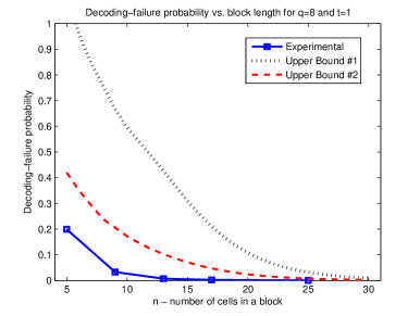
Figure 5: Upper bounds on the probability to fail decoding $1$ error in comparison with experimental results. Solid squared line - experimental results, dotted line - upper bound of Theorem 33, dashed line - upper bound of Theorem 38.

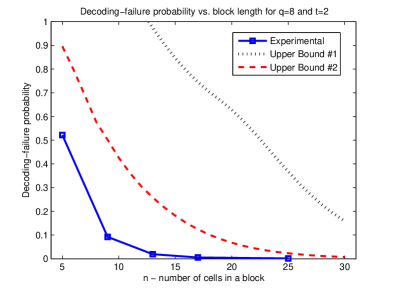
Figure 6: Upper bounds on the probability to fail decoding $2$ errors in comparison with experimental results. Solid squared line - experimental results, dotted line - upper bound of Theorem 33, dashed line - upper bound of Theorem 38.

VI The Q-ary Z-Channel Analysis

VI-A Capacity and capacity achieving distributions

A multi-level memory enduring asymmetric, magnitude-1 errors can be modeled by the $q$-ary Z-channel shown in Fig. 7. This channel is essentially Shannon’s noisy typewriter channel, only with a general transition probability $p$ and without the wrap-around transition from $0$ to $q-1$.

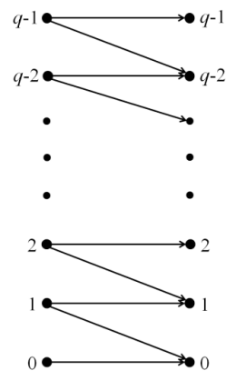
Figure 7: q-ary Z-channel model

A special case of this channel with $q=2$ is the binary Z-channel, which was extensively studied [14],[15]. Both the noisy typewriter channel and the binary Z-channel have analytic expressions for the channel capacity and for the corresponding input distributions. However, analyzing the $q$-ary Z-channel is more complicated, therefore, some numeric solutions must be used [16]. The capacity of the generalized probability $p$ noisy typewriter channel (with wrap-around) is given by

$$\mathrm{C}=1-h_{2}\left(p\right)\cdot log_{q}2,$$ (45)

where $h_{2}\left(p\right)$ is the binary entropy function. The capacity is achieved by the uniform input distribution. However, due to the symmetry break in the $q$-ary Z-channel (without wrap-around), calculating the capacity is more complicated, and the mutual information is given by

$$I\left(X;Y\right)=H\left(Y\right)-H\left(Y|X\right)=$$ (46)

$$-\sum_{y}p\left(y\right)log_{2}p\left(y\right)-\left(1-p\left(x=0\right)\right)\cdot h_{2}\left(p\right)$$

while $p\left(y\right)$ is given by

$$p\left(y\right)=\left\{\begin{array}[]{ll}p\left(x=0\right)+p\cdot p\left(x=1\right)&y=0\\ \left(1-p\right)\cdot p\left(x=q-1\right)&y=q-1\\ \left(1-p\right)\cdot p\left(x=y\right)+p\cdot p\left(x=y+1\right)&else\\ \end{array}\right.$$ (47)

We use optimization methods to find the input distribution $p\left(x\right)$ that maximizes the mutual information given in (47) and achieves the capacity of the channel. Fig. 8 presents the input distribution (for $q=7$) for several values of the error probability $p$. As can be noticed, when $p$ is very low, the capacity-achieving input distribution is relatively uniform. As $p$ increases, the lowest and highest levels become more probable. When $p$ is relatively high, the probability for the even levels increases and the probability for the odd levels decreases. When $p=0.5$, we get the well known zero-error code for the noisy typewriter channel called the all-even code previously in this paper. This only happens for odd $q$ values; for even $q$ the distribution converges to something non-uniform.

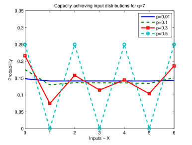
Figure 8: Capacity achieving input distributions for the q-ary Z-channel with q=7 and error probabilities of: $p=0.01$ - solid, $p=0.1$ - dashed, $p=0.3$ - solid & squares, $p=0.5$ - dashed & circles.

When we examine the symbol distribution of the NCC code, we see that it follows the capacity-achieving distributions of Fig. 8 in the following sense. An NCC code with length $n$ has a symbol distribution very close to the capacity-achieving distribution of the $q$-ary Z-channel with some error probability $p$. “Very close” means that the mutual information resulting from the NCC distribution is found numerically to be less than $0.01\%$ lower than the capacity. Note that this fact does not imply that the length $n$ NCC code achieves capacity for the corresponding probability $p$ channel. But Fig. 9 does give an indication that length $n$ NCC codes are well tuned to the corresponding probability $p$ channels. In the figure we plot for three lengths of NCC codes, $n=5,7,10$, the improvement in block-error rate (over uncoded) for each error probability $p$. On each plot we mark by a dot the $p$ parameter whose capacity-achieving distribution is closest to the NCC distribution. It can be seen that the best empiric error-correction performance of the NCC is achieved very close to these $p$ values found by the information-theoretic analysis.

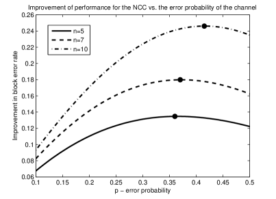
Figure 9: Block error rate improvent of the NCC vs. the error probability of the channel $p$. Solid line: $n=5$, dashed line: $n=7$, dash-dotted line: $n=10$. The dot on each plot marks the channel parameter $p$ for which the NCC distribution is closest to the capacity-achieving distribution.

VI-B Finite block-length analysis

NCC codes are attractive to use for finite lengths $n$ that depend on the channel parameter $p$. In the asymptotic regime where $n$ tends to infinity, it was shown in Section III that the NCC code converges to the even/odd code. Therefore, in order to evaluate the performance of the NCC code, we need to use finite block-length analysis tools. In the evaluation we use known results from the well-developed finite block-length information theory. In particular, we use the finite block-length upper bound (converse bound) first introduced by Strassen [17], and further refined and extended by Polyanskiy, Poor and Verdu [18], Tomamichel and Tan [19], and by Moulin [20]. We start with some formal definitions [18],[19].

Definition 39

. A $\left(n,M,\varepsilon\right)-code$ code is a length-$n$ code with $M$ codewords, for which there exists a decoder whose block error probability is smaller than $\varepsilon$.

The maximal code size achievable with block-length $n$ and error probability $\varepsilon$ is denoted by

$$M^{*}\left(n,\varepsilon\right)=\max\left\{M:\exists\>a\,\left(n,M,\varepsilon\right)-code\right\}.$$

Given that the capacity achieving input distribution is unique, the dispersion of the channel is defined as

$$V\triangleq\begin{array}[]{ll}Var\left[i\left(X,Y\right)|X\right],\end{array}$$ (48)

where $i\left(X,Y\right)$ is the information density given by

$$i\left(X,Y\right)=\log\frac{P_{Y|X}\left(y|x\right)}{P_{Y}\left(y\right)}.$$ (49)

Theorem 40

. [17]-[20] For every discrete memoryless channel (DMC) and $\varepsilon$ with $V\geqslant 0$, the following bound applies

$$\log M^{*}\left(n,\varepsilon\right)\leqslant nC-\sqrt{nV}\Phi^{-1}\left(\varepsilon\right)+\frac{1}{2}\log n+{\cal O}\left(1\right),$$ (50)

where $C$ is the Shannon capacity of the channel, and $\Phi\left(\cdot\right)$ is the Gaussian cumulative distribution function.

The channel dispersion $V$ of the $q$-ary Z-channel can be calculated using the capacity-achieving input distributions found by optimization tools in Section VI-A.

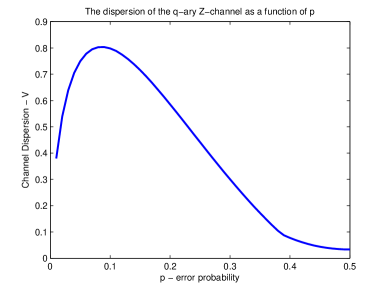
Figure 10: Channel dispersion $V$ of the $q$-ary Z-channel as a function of the error probability $p$.

Fig. 10 presents the channel dispersion as a function of the error probability of the channel. After finding $V$, (50) can be fully calculated. Comparing the NCC scheme with Theorem 40 is not straightforward and several remarks must be made. First, the fourth element of (50) may not be negligible for small values of $n$. Second, as can be seen in Table I, changing the block-length of the NCC inherently changes the error correction capability. Hence, the $n$ and $\varepsilon$ parameters are conjugated in the NCC scheme - meaning that for a given $q$-ary Z-channel with error probability $p=0.1$, using different block-lengths yields different $\varepsilon$’s. So, the way we compared the NCC to Theorem 40 is as follows. We fixed the error probability of the channel to $p=0.1$. Then we calculated (by exhaustive simulations) the resulting $\varepsilon$’s for four NCC block-lengths: $7,9,13,17$ (calculating it for higher values of $n$ demands serious computational resources). The calculated $\varepsilon$’s are $[0.0686,0.0407,0.0144,0.0054]$, respectively. Then, we calculated (50) for the four different values of $\varepsilon$.

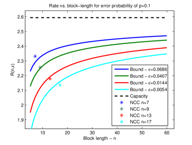
Figure 11: Solid lines - converse bounds for four values of $\varepsilon$, $[0.0686,0.0407,0.0144,0.0054]$. Stars - rates of the NCC for four values of $n$, $[7,9,13,17]$. Dashed horizontal line - the capacity of the channel for $p=0.1$.

Fig. 11 presents the comparison between the performance of the NCC and the converse bounds. As can be seen, for low values of $n$, the NCC beats the converse bound, which is possible because of the ${\cal O}\left(1\right)$ term in (50). As $n$ increases, we can see that the NCC nicely follows the bound, reaching rates that are $<1\%$ lower than the converse bounds. Therefore, the NCC code has the potential to be very close to optimal finite-block length for moderate block-length.

VII The NCC as an ECC Scheme in Flash Memories

Approaching the end of this paper, we want to venture beyond the theoretical discussion, and project the NCC scheme on the space of real flash storage devices. Given the attractiveness of the NCC in correcting asymmetric magnitude-1 errors (demonstrated in Fig. 4), it is natural to ask how to deploy it in real flash devices. In terms of computational complexity, we have provided in Section IV efficient algorithms for encoding and decoding NCC codewords. Thus there are two main issues left to resolve:

1. Coding over block lengths induced by large flash pages.

2. Correcting the residual errors at the decoder output.

It turns out that accomplishing item 1 is very easy, while item 2 is less immediate and is also a topic for further research.

To accommodate large flash pages (also called wordlines in the flash jargon), recall that the NCC block length $n$ determines both the code rate (decreasing with $n$) and the correction capability (improving with $n$). Typical block lengths shown to be useful/advantageous are from $n=5$ to $n\approx 30$. If we have flash pages of size $N\gg n$, then we simply concatenate $\lceil N/n\rceil$ parallel NCC codewords in each flash page, where the choice of $n$ is done based on the SER estimate and correction specifications for the device. A pictorial illustration is shown in Fig. 12. If the parameter $n$ is correctly chosen, each codeword will decode correctly, and a correct full page will be delivered to the user. By that we decouple the codeword length $n$ from the page size $N$.

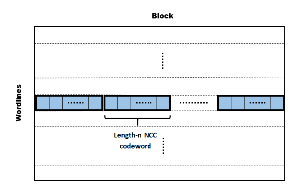
Figure 12: A memory block consisting of pages (wordlines), where each page includes concatenated length-$n$ NCC codewords.

To deal with residual errors at the NCC decoder output, we can concatenate it with an outer code for symmetric errors such as Reed-Solomon (RS) or LDPC code. If we use a RS code with alphabet size $M$ (the number of NCC codewords), then by standard concatenation an NCC decoding error will translate to a single symbol error in the RS code. Low decoding error probability can be achieved by the concatenated code so long that the NCC decoding-error probability (Table I) matches the correction capability of the RS code. For example, if we take an NCC code with $n=13$ on input SER $0.095$, then the resulting output SER is $0.0021$, which means that most of the NCC blocks will be decoded successfully, and then a high-rate RS code will suffice as the outer code. The more challenging aspect of residual errors is the treatment of secondary error types (e.g. the ones treated in [12]) in conjunction to the dominant asymmetric magnitude-1 errors. If these secondary errors are frequent enough to affect a significant fraction of NCC blocks, then the suggested concatenation with RS codes will not work, since many RS symbols would have residual errors left by the NCC decoder (which was not designed to combat these errors). In such cases, an alternative is to concatenate the NCC with an outer binary code, e.g. an LDPC code, and iterate information between the LDPC and NCC decoders such that the most likely codeword is found. That way, the redundancy from the LDPC code can help the NCC decoder prefer a more likely codeword, even if not all errors are asymmetric magnitude-1. Devising such a decoder is a topic for future work.

In the following example we demonstrate the potential benefit of concatenating an NCC code with an outer LDPC code, such that the symbols left in error by the NCC decoder (whose number is measured as SER in Fig. 4) are corrected by the LDPC code. The example shows that the SER reduction in asymmetric magnitude-1 errors offered by the NCC code allows using a low complexity LDPC decoder for the outer code, while alternative asymmetric magnitude-1 codes leave high output SER that cannot be corrected by an LDPC code of reasonable redundancy and complexity. We note that this example is for a quantitative illustration only, and not yet a working scheme, because it assumes that a single residual asymmetric magnitude-1 error maps to a single bit error at the LDPC decoder input. This assumption is not readily true, because of the non-trivial mapping between outer-code bits and NCC codewords (shown in Section IV-B).

Example 41

. The technical requirement for reliability of most flash memories stands on a bit-error rate (BER) of $10^{-15}$. Let us assume a $q=8$ flash memory suffers asymmetric magnitude-$1$ errors such that its raw (input) SER is $0.24$. The raw SER of $0.24$ is mapped to raw BER of approximately $0.08$, which is the SER level divided by the number of bits per symbol ($\log_{2}{q}=3$). An ECC scheme should be applied in order to reduce the relatively high raw BER of $0.08$ to a BER of $10^{-15}$, which is required by the consumer. Let us consider using state of the art LDPC codes designed for flash memories presented in [13] (Fig. 10). We can see that for a raw BER of $0.08$ none of the LDPC codes is useful. In fact, in order to reach a BER of $10^{-15}$ the raw BER of the strongest LDPC should be at most $0.013$. Let us now examine concatenating the LDPC codes with asymmetric magnitude-$1$ codes as inner codes. The asymmetric version of the BCH code reduces the raw BER of $0.08$ to $0.035$, which is not enough for the LDPC to converge. The even/odd scheme is slightly better, reducing the BER to $0.0203$, which is still insufficient. The NCC, however, reduces the raw BER of $0.08$ to $0.0065$, which can enable a soft LDPC with just two extra sensing levels to reach the required BER of $10^{-15}$.

VIII Conclusion and Future Work

The NCC flexible coding scheme for asymmetric magnitude-$1$ errors was presented. An optimal, low complexity decoding algorithm was introduced. The NCC was also analyzed and compared to BCH and even/odd codes, outperforming these codes for moderate to high values of SER. Several bounds on the error-correcting performance were derived. The NCC was also analyzed by finite block length analysis tools, indicating that this scheme has the potential to be nearly optimal.
For future work, it is possible to enhance the flexibility of the constraint and to expand the rate/correcting capabilities tradeoff. Furthermore, in order to address high error propagation when concatenating the NCC with some outer code, a more sophisticated and efficient concatenation method can de developed. On the theoretical side, developing sphere-packing bounds for the $q$-ary Z-channel may suggest additional analyses and refinements of the NCC. In addition, aside of correcting errors, the NCC can also be used for speeding up read and write processes in non-volatile memories.

IX Acknowledgment

The authors wish to thank Y. Polyanskiy for his guidance on the finite block-length analysis. This work was supported by the Israel Science Foundation, by the Israel Ministry of Science and Technology, and by a GIF Young Investigator grant.

Appendix A proof of Theorem 8

We prove Theorem 8 for the common scenario in which $q$ is an even number. The proof for the odd $q$ scenario is straightforward. This result is proved with the help of the following lemmas.

Definition 42

. A subcode of the NCC, $NCC_{r}\left(n,q\right)$ is a code containing all the codewords of $NCC\left(n,q\right)$ that occupy exactly $r$ levels. It is possible to define in a similar way the subcode $even/odd_{r}\left(n,q\right)$ of the even/odd code.

Lemma 43

. The information rates of $NCC_{q/2}\left(n,q\right)$ and $even/odd_{q/2}\left(n,q\right)$ are identical when $n\rightarrow\infty$.

Proof.

From Theorem 7 we know that when the number of occupied levels in a codeword is $q/2$, which is the maximal value of occupied levels, there are $q/2+1$ combinations of levels for an NCC codeword, while there are only two for the even/odd code ($[0,2,\ldots,q-2]$ or $[1,3,\ldots,q-1]$). Let us denote by $M$ the number of $even/odd_{q/2}\left(n,q\right)$ codewords. The number of $NCC_{q/2}\left(n,q\right)$ codewords is therefore $\frac{q/2+1}{2}M$, so the information rate in this case is

$${\cal R}_{NCC}=log_{q}\left(\frac{q/2+1}{2}M\right)/n={\cal R}_{even/odd}+log_{q}\left(\frac{q/2+1}{2}\right)/n,$$ (51)

Therefore, it is clear that when $q/2$ levels are occupied and $n\rightarrow\infty$ the information rates of the NCC and even/odd schemes are identical.   

Lemma 44

. When we uniformly select an $NCC(n,q)$ codeword, the probability $Prob\left(n,q/2\right)$ for selecting a $NCC_{q/2}\left(n,q\right)$ codeword is asymptotically $1$ when $n\rightarrow\infty$. In other words, when $n$ is large, the subcode $NCC_{q/2}\left(n,q\right)$ and the $NCC\left(n,q\right)$ code coincide.

Proof.

From the proof of Theorem 7 it is clear that the probability $Prob\left(n,q/2\right)$ to choose $n$-length, $q/2$ occupied levels codeword is given by:

$$Prob\left(n,\frac{q}{2}\right)=\frac{\frac{q}{2}!\cdot S\left(n,\frac{q}{2}\right)\cdot\left(\frac{q}{2}+1\right)}{\sum_{k=1}^{\frac{q}{2}}k!\cdot S\left(n,k\right)\cdot\binom{q-k+1}{k}}$$ (52)

Recall that asymptotically $S\left(n,k\right)\sim\frac{k^{n}}{k!}+{\cal O}\left((k-1)^{n}\right)$, therefore we get

$$Prob\left(n,\frac{q}{2}\right)\sim\frac{\left(\frac{q}{2}\right)^{n}\cdot\left(\frac{q}{2}+1\right)}{\sum_{k=1}^{\frac{q}{2}-1}k^{n}\cdot\binom{q-k+1}{k}+\left(\frac{q}{2}\right)^{n}\cdot\left(\frac{q}{2}+1\right)}$$ (53)

After some algebra we get:

$$Prob\left(n,\frac{q}{2}\right)\sim\frac{1}{\sum_{k=1}^{\frac{q}{2}-1}\left(\frac{2k}{q}\right)^{n}\cdot\binom{q-k+1}{k}/\left(\frac{q}{2}+1\right)+1}$$ (54)

Due to the fact that for the relevant values of $k$, we get $\frac{2k}{q}<1$ and that $\binom{q-k+1}{k}/\left(\frac{q}{2}+1\right)$ is bounded and does not depend on $n$ it is obvious that

$$\lim_{n\rightarrow\infty}Prob\left(n,\frac{q}{2}\right)=1$$ (55)

 

When $n\rightarrow\infty$ it is clear by (2) that ${\cal R}_{even/odd}\rightarrow{\cal R}_{all-even}$. From Lemmas 43 and 44 it is clear that the information rates of the NCC and even/odd are the same.

References

- [1] N. Mielke, T. Marquart, N. Wu, J. Kessenich, H. Belgal, E. Schares, F. Trivedi, E. Goodness and L. Nevill “Bit error rate in NAND flash memories,” in Proc. of IEEE Int. Reliability Physics Symp. (IRPS), pp.9-19, April 2008.
- [2] Y. Cai, E. Haratsch, O. Mutlu and K. Mai “Error patterns in MLC NAND flash memory: Measurement, characterization, and analysis,” in Proc. of IEEE Design, Automation & Test in Europe Conference & Exhibition (DATE), pp.521-526, March 2012.
- [3] R. Ahlswede, H. Aydinian, and L. Khachatrian, “Unidirectional error control codes and related combinatorial problems,” in Proc. of the Eighth Int. Workshop on Algebraic and Combinatorial Coding Theory (ACCT-8), St. Petersburg, Russia ,pp.6-9, 2002.
- [4] Y. Cassuto, M. Schwartz, V. Bohossian and J. Bruck “Codes for asymmetric limited-magnitude errors with application to multi-level flash memories,” IEEE Trans. Inform. Theory, vol. 56, no. 4, pp.1582-1595, 2010.
- [5] A. Jiang, Y. Li and J. Bruck “Bit-fixing codes for multi-level cells,” in Proc. of IEEE Information Theory Workshop (ITW), pp.252-256, Sept. 2012.
- [6] L.G. Tallini and B. Bose, “On L1-distance error control codes,” in Proc. of IEEE Int. Symp. on Inform. Theory, ISIT, pp.1061-1065, July 2013.
- [7] E. Hemo and Y. Cassuto, “A Constraint Scheme for Correcting Massive Asymmetric Magnitude-1 Errors in Multi-Level NVMs,”in Proc. of IEEE Int. Symp. on Information Theory (ISIT), June 2015.
- [8] J. van Lint and R. Wilson, A Course in Combinatorics, second edition. Cambridge University Press, 2001.
- [9] A. Mohr and T.D. Porter, “Applications of Chromatic Polynomials Involving Stirling Numbers, ” Journal of Combinatorial Mathematics and Combinatorial Computing, vol. 70, pp. 57-64, Aug. 2009.
- [10] L. Comtet, Advanced Combinatorics. Reidel, Dordrecht, 1974.
- [11] F.T. Howard, “Associated Stirling numbers,” Fibonacci Quart., vol 18 (4), pp. 303-315, Dec. 1980.
- [12] Y. Li, E. Gad, A. Jiang and J. Bruck, “Data archiving in 1x-nm NAND flash memories: Enabling long-term storage using rank modulation and scrubbing,” in IEEE International Reliability Physics Symposium (IRPS), pp.6C-6, 2016.
- [13] K. Zhao, W. Zhao, H. Sun, T. Zhang, X. Zhang and N. Zheng “LDPC-in-SSD: making advanced error correction codes work effectively in solid state drives,” In Proc. of the 11th USENIX conference on File and Storage Technologies (FAST’13), pp.243-256, 2013.
- [14] S. W. Golomb, “The limiting behavior of the Z-channel,” IEEE Trans. Inform. Theory, vol. IT-26, pp.372, May 1980.
- [15] L. G. Tallini, S. Al-Bassam and B. Bose, “Feedback codes achieving the capacity of the Z-channel,” IEEE Trans. Inform. Theory, vol.54, no.3, pp.1357-1363, 2008.
- [16] N. Shulman and M. Feder, “Communication over an unknown channel via common broadcasting,” Ph.D. dissertation, Faculty of EE - Systems, Tel-Aviv University, Tel Aviv, Israel, June 2003.
- [17] V. Strassen, “Asymptotische Abschätzungen in Shannons Informationstheorie,” In Trans. Third Prague Conf. on Inform. Theory, pp.689-723, Prague, 1962.
- [18] Y. Polyanskiy, H.V. Poor and S. Verdu, “Channel Coding Rate in the Finite Blocklength Regime,” IEEE Trans. Inform. Theory, vol.56, no.5, pp.2307-2359, 2010.
- [19] M. Tomamichel and V.Y.F. Tan, “A Tight Upper Bound for the Third-Order Asymptotics for Most Discrete Memoryless Channels,” IEEE Trans. Inform. Theory, vol.59, no.11, pp.7041-7051, 2013.
- [20] P. Moulin, “The log-volume of optimal constant-composition codes for memoryless channels, within O (1) bits,” in Proc. of IEEE Int. Symp. on Inform. Theory, ISIT, pp.826-830, July 2012.
- [21] M. Riedel, Number of ways to partition a set with n elements to k subsets where at least one subset has r elements, URL (version: 2013-10-22): https://math.stackexchange.com/q/535146.