Nonlinear fiber gyroscope for quantum metrology
Abstract
We examine the performance of a nonlinear fiber gyroscope for improved signal detection beating the quantum limits of its linear counterparts. The performance is examined when the nonlinear gyroscope is illuminated by practical field states, such as coherent and quadrature squeezed states. This is compared with the case of more ideal probes such as photon-number states.
pacs:
03.65.-w, 42.50.St, 42.50.LcI Introduction
Signal-detection strategies based on nonlinear processes can clearly outperform current strategies based on linear processes LU04 ; BFCG07 ; BDDFSC08 ; BDDSTC09 ; GZNEO10 ; NM10 ; TBDSC10 ; RL10 ; LU10 ; NKDBSM11 ; SNBCCM14 ; LR15 ; JLZLBBNDW13 . This is so even when using probes in classical-like states. This is relevant because classical-like states are characterized by their robustness against practical imperfections, that can be deadly for schemes using probes prepared in nonclassical states HMPEPC97 ; DBS13 ; DJK14 .
A suitable arena for nonlinear detection schemes is optics. The most precise detection schemes are optical interferometers, and nonlinear processes are quite simply implemented in optics via propagation in nonlinear media.
In this work we focus on the quantum limits to the resolution achievable in gyroscopes as good candidates to exploit the benefits of nonlinear detection, paying special attention to quantum characteristics exclusive of this interferometer GY . We will focus on the case when the gyroscope is illuminated by practical field states, i. e., that can be generated in practice and are robust against imperfections, such as coherent and quadrature squeezed states. For the sake of comparison the results will be compared with the case of probes in less practical states, such as product of number states.
There are two important advantages in the proposed scheme with respect to other nonlinear detection schemes, namely, its improved optical performance and its capability to measure angles. More specifically, as a comparison with other interferometers (like Michelson’s) nonlinearity is integrated as a constituent part of the gyroscope, so that it is not necessary to modify the set up to include extra elements to provide the nonlinear effect. For instance, in order to include nonlinearity in the LIGO gravitational-wave detector we should “attach” some nonlinear material to it LIGO . The simplest way to do this would be by filling the room with a nonlinear gas. This will produce severe practical inconvenient since gases are a reported source of technical noise because of density fluctuations and light scattering, which is the reason why LIGO works at ultra-hight vacuum. Furthermore the nonlinearity in gases is typically small. An alternative would be to attach a piece of nonlinear material to the suspended masses. In such a case some light will be reflected in the interphase and in any case it far for technically simple to make such attachments because of the large dimensions of the device. Our proposal is free of these problems because the nonlinearity is automatically embedded as a part of the interferometer: the optical fiber. The optical performance of fiber glasses is much superior than gases regarding homogeneities and any other source of scattering and fluctuations. Moreover, the nonlinear effect is much larger than for gases, being improved by the very large electric fields that can be reached by light confinement in the small volumes of the fiber core. Gyroscopes do not need to be kilometer long devices to provide extremely long optical paths required for precision interferometry since looped fiber-optics coil multiplies the length and the cumulative effects of nonlinearlity by the number of loops. Finally, the gyroscope is a rigid detector without moving parts, that always provides a more robust and improved optical performance.
On the other hand, up to our knowledge nobody has considered to apply nonlinear quantum metrology in a gyroscopic scheme. This is very timely because there are many interesting unobserved effects caused by rotations, specially to test gravitational theories and phenomena. For example, the Lense-Thirring effect, a relativistic effect not observed yet, the local space-time curvature, or the existence of a preferred frame in the Universe OZ .
Besides fiber-optics realizations, previous works have shown that nonlinear interferometers are feasible in other physical contexts, such as Bose-Einstein condensates BDDFSC08 ; BDDSTC09 ; GZNEO10 ; TBDSC10 ; JD and nanomechanical resonators WMC . Finally, we may point out that gyroscopes share geometry with sensors sensible to physical variables different from rotations and involving relevant physical phenomena such as the Aharonov-Bohm effect for example GDR .
II Model
Any detection scheme involves four steps. In the first one, some probe state is prepared. In the second step the probe experiences a signal-dependent transformation . Then, the measurement of some observable is performed at the output state of the probe . With the results of the measurement the signal and its uncertainty are estimated.
II.1 Probe and system modes
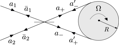
The probe is the light state illuminating the gyroscope. Within the interferometer the system is made of two counter-propagating modes with complex-amplitude operators , that can be feed trough a lossless 50 % beam splitter coupling the inner modes with two input modes (see Fig. 1)
| (1) |
The probes are prepared in modes while the observation will be made at the output modes leaving the gyroscope. These are related to the modes within the interferometer through a beam splitter performing the transformation inverse to the one in Eq. (1)
| (2) |
where are the amplitudes at the end of the nonlinear fiber, while refer to the amplitudes at the beginning.
II.2 Signal-dependent transformation
In the second step the probe experiences a signal-dependent transformation . The rotation of the gyroscope introduces an asymmetry between the times spent by the two modes within the interferometer, that leads to a phase-difference
| (3) |
where is the field frequency, is the length of the fiber, is the area enclosed by a single loop of the fiber made of loops of radius , is the number of loops, is the angular speed, are the indices of refraction for the corresponding modes, and we have assumed that the speed acquired by the fiber due to is much smaller than the speed of light in vacuum .
The key point for our work is that we are dealing with nonlinear media so the indices of refraction depend on the light intensities. Assuming Kerr-type nonlinearity and light traveling as pulses of frequency , cross-section , and duration , carrying a number of photons , we will have
| (4) |
where is the linear index, are the nonlinear susceptibilities, for simplicity the medium is assumed optically isotropic so that the linear index is the same for both modes, are the electric-field strengths, and is the magnetic permeability of the vacuum. The second equality in Eq. (4) is just a rough approximation to motivate the ongoing quantum analysis. We have assumed that there are no crossed terms. This is specially so in a pulsed illumination since in such a case the overlap of the counter propagating pulses is negligible.
In the quantum analysis, the propagation of the modes within the fiber can be described by the unitary operator , where includes all the signal-dependent effects given by the second term on the right-hand side of Eq. (3), while contains the contributions independent of , this is the contribution of the first term on the right-hand side of Eq. (3). The factorization is possible because both parts can be fully expressed in terms of two commuting phase shifts generated by different powers of the photon-number operators.
In this work we focus on the nonlinear part of the signal-dependent component . The contribution by will be invoked just to introduce and additional fixed phase when necessary. Otherwise, it will be assumed embodied in the probe preparation or compensated by a similar amount of fiber propagation not experiencing the rotation.
For the signal-dependent part we will just consider the nonlinear contribution given by the second term on the right-hand side of Eq. (4). This should be the dominating part for sufficiently large photon numbers, as far as we intend to exploit the asymptotic behavior allowed by nonlinear effects. In any case, the phase shifts produced by the linear and nonlinear parts of the transformation may be addressed simultaneously via a multi-parameter estimation procedure Ch . This is studied in more detail in Appendix B showing that it agrees with the expected results both for the linear and nonlinear parts.
Thus, the signal-dependent transformation we are going to study is
| (5) |
where are the corresponding number operators and the signal takes the form , assuming the nonlinear susceptibilities identical for both modes . Note that the relative sign in Eq. (5) is the correct one for counter-propagating modes. The sing depending on the propagation direction is often expressed by saying that for counter-propagating modes the generator is proportional to momentum rather than to energy mg .
Using Eq. (1) we find an useful expression for the generator , in terms of the input modes by
| (6) |
where is the total-number operator
| (7) |
and we have used that is a conserved quantity at the beam splitter. We note that the second equality in (6) is formally the same generator already tested experimentally in Ref. NKDBSM11 in a very different context.
II.3 Measurement
The most simple measurement sensitive to signals encoded as phase shifts is the interference achieved by the coupling at the beam splitter of the modes after the nonlinear propagation, , followed by photon-number detection at the outgoing beams . This provides us with a photon-number statistics containing the complete information about the signal available in this arrangement. In order to extract this information the most simple option is to consider the difference between the output photon numbers as . Since the transformation (5) is quite simple we have the following expression for in terms of the complex amplitudes at the beginning of the fiber
| (8) |
and is any fixed additional linear phase shift introduced to optimize performance. Then, we can express in terms of the input modes via Eq. (1) as
| (9) |
where , .
For the most simple situations the lowest-order moments of may be enough. However, there are situations where they may not extract most of the signal information encoded in the output field state. In such situations we may look at the complete output photon-number statistics in order to better understand the situation.
II.4 Simple estimation
The key performance estimator is the signal uncertainty . In a very simple first approach this can be estimated from the lowest-order moments of via the signal to noise ratio, or, equivalently, from a simple error propagation as:
| (10) |
where in the last inequality the uncertainty relation has been used. In some relevant situations optimum results are obtained if so that for very small signals will be near zero, which is the point of maximum sensitivity to phase variations. In such a case for we have after Eqs. (9), (5), and (6)
| (11) |
and
| (12) |
At this stage one might be tempted to look for optimum results in terms of minimum uncertainty states of and , granting the equality in the last step in Eq. (10). However, this is not quite so optimum strategy since some other probes may lead to smaller via a larger even though they are not minimum DA .
II.5 Advanced estimation
The estimation of the uncertainty can be addressed using more powerful tools such as the Cramér-Rao lower bound and the quantum Fisher information as Fi
| (13) |
where is the Fisher information
| (14) |
with and standing for the pair of natural numbers representing the number of photons registered at the two outputs of the gyroscope. In the case of no additional phase shift the output photon-number statistics is
| (15) | |||||
where is the unitary operator representing the action of the input beam splitter, are number states, and we have taken into account that the output beam splitter performs the inverse transformation of the input.
In the case that the probe is in a pure state with real coefficients in the number basis , then , with and it can be easily shown that DDLP
| (16) |
where in the last step we have used that if then after Eq. (6) .
Naturally the fact that the full photon number statistics outperforms those of the simple measurement of is rather obvious since the statistics of is a marginal of the full statistics . The key point here is that when the probe state has real coefficients in the number basis, the statistics contains all the information conveyed by the transformed probe state so that its Fisher information equals the quantum Fisher information. Note that this conclusion holds for all . Since the total-number variable does not provide phase information, all the phase information in is actually provided by . As we shall see, in many cases of interest the two lowest-order moments of already contain all the relevant information about .
III Quantum resolution for different probes
Typically, decreases as the mean number of photons in the probe state increases. So the usual task is to look for the minimum at fixed , this is to say, minimum uncertainty at fixed energy resources. Alternatively, this is to inquire about the probe states that provide the best scaling of as a function of . To this end we will consider different probe states under the two estimation uncertainties in Secs. IID and IIE.
III.1 Product of coherent states
If the input probe is in a product of Glauber coherent states , the field state in modes will be as well a product of coherent states with the same total mean number of photons . A simple calculus leads exactly to
| (17) |
while
| (18) |
where and we have assumed real . Typically is small enough so that and . Moreover, will take advantage of the robustness of coherent states to consider a large mean number of photons .
We can observe that the dispersion of total number of photons in the coherent state degrades the visibility of the interference through the factor . Therefore, in order to obtain meaningful results it is convenient to assume that . This is to say that the signal expected is below the standard quantum limit, so it would pass unnoticed if the fiber were linear. In such a case, we have for
| (19) |
and for all , so that after Eq. (10)
| (20) |
The optimum result holds for small enough signals well below the Heisenberg limit of linear devices so that . When varying the balance of photons between the modes, the minimum uncertainty holds for an equal splitting of resources between the fiber modes, this is so that with a coherent state in mode and vacuum in mode . With all this we get
| (21) |
Note that is quite below the standard quantum limit and the Heisenberg limit of linear devices, so the result is consistent with the approximations made.
If we go beyond the simple estimation we have that the probe has real coefficients in the number basis. So, if now we consider , we get to the leading order in for all . As a bonus we get that the intense coherent states behave as minimum uncertainty states for the , pair.
III.2 Product of coherent and squeezed states
The benefits of using squeezed states in linear quantum metrology are well-known from a long time ago sv0 ; sv1 ; sv2 . We can check whether a similar result holds in the nonlinear case. To show this in the simplest manner we consider as probe state in mode a coherent state with real and and squeezed vacuum in mode with squeezing parameter and mean number of photons . Again we consider a fixed mean total number of photons with .
We begin with the simple evaluation of in Eq. (10) for and . For the choice of the squeezing direction to reduce fluctuations of the quadrature we have after Eq. (11)
| (22) |
and from Eq. (12)
| (23) |
with
| (24) |
For and it can be readily seen that the minimum in Eq. (10) holds for , leading to
| (25) |
Comparing Eqs. (21) and Eq. (25) we see that squeezing provides an effective improvement of resolution over the pure coherent case. Moreover, after noting that in these conditions we get that the probe is close to be a minimum uncertainty states of the pair , since is twice the minimum .
In Appendix A we have carried out an analysis of errors in the presence of several sources of noise that can be readily accounted for by the replacement in the detection operator in Eq. (11)
| (26) |
where is a random phase Gaussian distributed with zero mean and variance , is the quantum efficiency of the detectors, and are uncorrelated field modes in thermal states carrying photons with . The signal uncertainty becomes
| (27) |
The dominant factor are the fluctuations of the relative phase that would spoil the improvement caused by the squeezing vacuum unless . The other two terms would tend to phase uncertainty similar to the case of pure coherent probes unless .
After the tools in Sec. IIE we can go beyond taking into account that when is real and when the squeezing takes place either in the quadrature or in , the coefficients of the probe state in the number basis are real so that . Then we can ask for the balance between and that leads to maximum at fixed . For we can neglect the fluctuations in mode . Moreover, for we can carry our the following approximation for the squeezed mode where is a Gaussian variable with and . In this limit it can be readily seen that the optimum result is that holds for , so that for every
| (28) |
Comparing Eqs. (25) and (28) we can appreciate that the resolution provided by the complete number statistics outperforms the simple estimation after the measurement of . This can be regarded as a generalization to nonlinear interferometry of the result for the linear case in Ref. sv2 . It is also worth noting that both in the linear and nonlinear schemes optimum results are obtained for the same probe states. The only difference is the amount of squeezing, 50 % in the linear case versus 70 % in the nonlinear one. This is to say that nonlinearity offers resolution improvement without any drawback in the probe preparation.
III.3 Product of number states
The above cases refer to realistic probe states. This can be compared with more ideal probes, such as the product of number states with . Starting with the simple estimator in Eq. (10) and using the complete exact expression Eq. (9) we get
| (29) |
and
| (30) |
where , , so that for any and
| (31) |
The minimum uncertainty holds either when or , so that for large the uncertainty scales as
| (32) |
This input probe is an SU(2) coherent state, which are the projection on fixed total number of the standard coherent states AD . Accordingly the resolution is the same reached with coherent probes in Eq. (21). However, note that in this case the result holds for all because here there is no dispersive effect caused by the fluctuations of . Beyond this minimum, the uncertainty (31) grows without limit as approaches . Deep down this holds because for we get that no longer depends on the signal .
Regarding the more advanced estimation provided by the complete statistics , we get the opposite conclusions. After the Fisher information the minimum uncertainty holds for as close as possible to , this is for even , which is the well-known case of twin photon states HB . This leads to and
| (33) |
On the other hand, the minimum holds for the SU(2) coherent states with in agreement with Eq. (32).
In this particular case, it is possible to reach the optimum resolution (33) via the simple estimation procedure considering that the measured observable is instead of . To simplify the calculation we consider from the start the probe with for even . In such a case
| (34) |
and
| (35) |
Considering and we get finally
| (36) |
reaching the minimum value predicted by the Cramér-Rao bound in Eq. (33). Incidentally with the above computations it can be easily checked that the product of twin number states tend to be minimum uncertainty states of the pair , for as , this is .
IV Conclusions
We have examined the performance of nonlinear gyroscopes in the quantum regime that highlight some relevant features for quantum metrology. This schemes does not imply length variations, so that this can be a built-in solid detector where all the potential advantages of nonlinearity can be used without the drawbacks caused if lengths were allowed to vary. Then the interferometer can be made of optical fibers where length and field confinement can be much improve the nonlinear effects.
A key result is that the optimum resolution can be approached by feasible coherent-squeezed inputs. This is a translation to nonlinear detection of the same result already proved for linear schemes. We find remarkable that in this non-linear scheme where the linear and non-linear propagations commute the benefits of nonlinear schemes can be obtained for the same probe states of the linear interferometry. However this may not be the case if the corresponding generators do not commute.
Acknowledgements
We thank Prof. L. Pezzé for helpful comments. We acknowledge financial support from Spanish Ministerio de Economía y Competitividad Projects No. FIS2012-33152 and No. FIS2012-35583 and from the Comunidad Autónoma de Madrid research consortium QUITEMAD+ Grant No. S2013/ICE-2801.
Appendix A Noise analysis
For completeness let us address a simple but meaningful analysis of the effect of unavoidable sources of noise, such as finite quantum efficiency, thermalization and phase randomization. To be more specific, we focus on the cases of pure coherent and coherent-squeezed probes since they provide the most interesting, meaningful and practical of the situations studied above. Several sources of noise can be readily accounted for by the replacement in the detection operator in Eq. (11)
| (37) |
where is a random phase that we will assume to be Gaussian distributed with zero mean and variance , is the quantum efficiency of the detectors, and are uncorrelated field modes in thermal states with , and with , respecting that quantum efficiency and thermalization are independent sources of uncertainty.
In such a case for probes in the product of coherent and squeezed states we have that in the absence of signal
| (38) |
where is the coherent amplitude assumed real. Taking into account that in our case , , assuming , and considering the optimum case where the number of photons in the squeezed state is , we get
| (39) |
where , while for the denominator in Eq. (10) we have just . Therefore the final form for the signal uncertainty becomes
| (40) |
The most potentially harmful is the last term caused by the fluctuations of the relative phase . This is natural because variations of cause that the coherent field couples with the anti-squeezed component of the vacuum mode , so the planned squeezing reduction becomes actually noise amplification. This effect would spoil the improvement caused by the squeezing vacuum unless . The other two terms in are due to finite quantum efficiency and thermal photons, and would tend to phase uncertainty similar to the case of pure coherent probes unless .
On the other hand, for the case of pure coherent probes we get that the uncertainty preserves the scaling
| (41) |
in accordance with the robustness of coherent light.
Appendix B Linear and nonlinear phase shifts
A relevant characteristics of the propagation in optically nonlinear media is that the field experiences always both linear and nonlinear effects. This raises a very interesting question regarding which transformation will encode optimally the signal, and whether its performance would be affected by the presence of the other one. The proper arena to examine this issue is a multi-parameter estimation procedure Ch . More specifically, if the signal-dependent transformation is
| (42) |
lower bounds for the estimation of and can be obtained in terms of the quantum Fisher information matrix as
| (43) |
as
| (44) |
In our case we have
| (45) |
with . Since we are dealing with quantum Fisher information we may follow the same approximations leading to Eq. (28).
After an straightforward calculation we finally get that for fixed mean total photon number the optimum holds for leading to which is rather close to the Heisenberg limit .
On the other hand the optimum holds for leading to which is also rather close to Eq. (28). Therefore, we may say that the multi-parameter protocol reproduces expected results for the estimation of linear and nonlinear phase shifts which seem to be not affected by the presence of the other part.
We have carried out the same analysis for the case when there is no squeezing so the mode is in the plain vacuum state leading to, in the limit , to and . So in comparison with the squeezed case the conclusion would be the opposite in the sense that there would be a clear perturbation between linear and nonlinear estimation processes, as already encountered in an slightly different single-mode nonlinear detector scheme Ch .
References
- (1) A. Luis, Nonlinear transformations and the Heisenberg limit, Phys. Lett. A 329, 8 (2004).
- (2) S. Boixo, S. T. Flammia, C. M. Caves, and J. M. Geremia, Generalized limits for single-parameter quantum estimation, Phys. Rev. Lett. 98, 090401 (2007).
- (3) S. Boixo, A. Datta, M. J. Davis, S. T. Flammia, A. Shaji, and C. M. Caves, Quantum Metrology: Dynamics versus Entanglement Phys. Rev. Lett. 101, 040403 (2008).
- (4) S. Boixo, A. Datta, M. J. Davis, A. Shaji, A. B. Tacla, and C. M. Caves, Quantum-limited metrology and Bose-Einstein condensates, Phys. Rev. A 80, 032103 (2009).
- (5) C. Gross, T. Zibold, E. Nicklas, J. Estéve, and M. K. Oberthaler, Nonlinear atom interferometer surpasses classical precision limit, Nature 464, 1165 (2010).
- (6) M. Napolitano and M. W. Mitchell, Nonlinear metrology with a quantum interface, New J. Phys. 12, 093016 (2010).
- (7) A. B. Tacla, S. Boixo, A. Datta, A. Shaji, and C. M. Caves, Nonlinear interferometry with Bose-Einstein condensates, Phys. Rev. A 82, 053636 (2010).
- (8) A. Rivas and A. Luis, Precision quantum metrology and nonclassicality in linear and nonlinear detection schemes, Phys. Rev. Lett. 105, 010403 (2010).
- (9) A. Luis, Quantum-limited metrology with nonlinear detection schemes, SPIE Reviews 1, 018006 (2010).
- (10) M. Napolitano, M. Koschorreck, B. Dubost, N. Behbood, R. J. Sewell, and M. W. Mitchell, Interaction-based quantum metrology showing scaling beyond the Heisenberg limit, Nature 471, 486 (2011).
- (11) R. J. Sewell, M. Napolitano, N. Behbood, G. Colangelo, F. Martin Ciurana, and M. W. Mitchell, Ultrasensitive atomic spin measurements with a nonlinear interferometer, Phys. Rev. X 4, 021045 (2014).
- (12) A. Luis and A. Rivas, Nonlinear Michelson interferometer for improved quantum metrology, Phys. Rev. A 92, 022104 (2015).
- (13) X. Jin, M. Lebrat, L. Zhang, K. Lee, T. Bartley, M. Barbieri, J. Nunn, A. Datta, and I. A. Walmsley, Surpassing the conventional Heisenberg limit using classical resources, CLEO: QELS Fundamental Science 2013, San Jose, CA, OSA Technical Digest (online) (OSA, Washington, D.C., 2013), paper QF2B.2 (2013).
- (14) S. F. Huelga, C. Macchiavello, T. Pellizzari, A. K. Ekert, M. B. Plenio, and J. I. Cirac, Improvement of frequency standards with quantum entanglement, Phys. Rev. Lett. 79, 3865 (1997).
- (15) R. Demkowicz-Dobrzański, K. Banaszek, and R. Schnabel, Fundamental quantum interferometry bound for the squeezed-light-enhanced gravitational wave detector GEO 600, Phys. Rev. A 88, 041802(R) (2013).
- (16) R. Demkowicz-Dobrzański, M. Jarzyna, and J. Kołodyński, Quantum limits in optical interferometry, Prog. Opt. 60, 345 (2015).
- (17) K. U. Schreiber and J.-P. R. Wells, Large ring lasers for rotation sensing, Rev. Sci. Instrum. 84, 041101 (2013).
- (18) B. P. Abbott et al. (LIGO Scientific Collaboration and Virgo Collaboration), Observation of Gravitational Waves from a Binary Black Hole Merger, Phys. Rev. Lett. 116, 061102 (2016).
- (19) M. O. Scully and M. S. Zubairy, Quantum Optics (Cambridge University Press, Cambridge, England, 1997).
- (20) L. M. Rico-Gutierrez, T. P. Spiller, and J. A. Dunningham, Quantum-enhanced gyroscopy with rotating anisotropic Bose Einstein condensates, New J. Phys. 17, 043022 (2015).
- (21) M. J. Woolley, G. J. Milburn and C. M. Caves, Nonlinear quantum metrology using coupled nanomechanical resonators New J. Phys. 10, 125018 (2008).
- (22) C. González-Santander, F. Domínguez-Adame, and R. A. Römer, Excitonic Aharonov-Bohm effect in a two-dimensional quantum ring Phys. Rev. B 84, 235103 (2011)
- (23) J. Cheng, Quantum metrology for simultaneously estimating the linear and nonlinear phase shifts, Phys. Rev. A 90, 063838 (2014).
- (24) M. Toren and Y. Ben-Aryeh, The problem of propagation in quantum optics, with applications to amplification, coupling of EM modes and distributed feedback lasers, Quantum Opt. 6, 425 (1994); J. Reháček, L. Mišta Jr., and J. Peřina, Codirectional simulation of contradirectional propagation, J. Mod. Opt. 46, 801 (1999); J. Peřina Jr. and J. Peřina, Quantum statistics of nonlinear optical couplers, Prog. Opt., 41, 361 (2000); A. Lukš and V. Peřinová, Canonical quantum description of light propagation in dielectric media, Prog. Opt. 43, 295 (2002).
- (25) D. Maldonado-Mundo and A. Luis, Metrological resolution and minimum uncertainty states in linear and nonlinear signal detection schemes, Phys. Rev. A 80, 063811 (2009).
- (26) C. W. Helstrom, Minimum mean-squared error of estimates in quantum statistics, Phys. Lett. A 25, 101 (1967); The minimum variance of estimates in quantum signal detection, IEEE Trans. Inform. Theory IT-14, 234 (1968); Quantum Detection and Estimation Theory (New York: Academic, 1976) S. L. Braunstein and C. M. Caves, Statistical distance and the geometry of quantum states, Phys. Rev. Lett. 72, 3439 (1994).
- (27) V. Peřinová , A. Lukš, and J. Křepelka, States of the optimum Fisher measure of information for quantum interferometry, Phys. Rev. A 73, 063807 (2006); G. A. Durkin and J. P. Dowling, Local and global distinguishability in quantum interferometry, Phys. Rev. Lett. 99, 070801 (2007).
- (28) C. M. Caves, Quantum-mechanical noise in an interferometer, Phys. Rev. D 23, 1693 (1981); M. Xiao, L.-A. Wu, and H. J. Kimble, Precision measurement beyond the shot-noise limit, Phys. Rev. Lett. 59, 278 (1987); P. Grangier, R. E. Slusher, B. Yurke, and A. LaPorta, Squeezed-light enhanced polarization interferometer, Phys. Rev. Lett. 59, 2153 (1987); LIGO Scientific Collaboration, A gravitational wave observatory operating beyond the quantum shot-noise limit, Nat. Phys. 7, 962 (2011); LIGO Scientific Collaboration, Enhanced sensitivity of the LIGO gravitational wave detector by using squeezed states of light, Nat. Photonics 7, 613 (2013).
- (29) A. Monras, Optimal phase measurements with pure Gaussian states, Phys. Rev. A 73, 033821 (2006); M. D. Lang and C. M. Caves, Optimal quantum-enhanced interferometry using a laser power source, Phys. Rev. Lett. 111, 173601 (2013).
- (30) L. Pezzé and A. Smerzi, Mach-Zehnder interferometry at the Heisenberg limit with coherent and squeezed-vacuum light, Phys. Rev. Lett. 100, 073601 (2008).
- (31) P. W. Atkins and J. C. Dobson, Angular momentum coherent states, Proc. R. Soc. London, Ser. A 321, 321 (1971).
- (32) M. J. Holland and K. Burnett, Interferometric detection of optical phase shifts at the Heisenberg limit, Phys. Rev. Lett. 71, 1355 (1993); T. Kim, J. Shin, Y. Ha, H. Kim, G. Park, T. G. Noh, and C. K. Hong, The phase-sensitivity of a Mach Zehnder interferometer for the Fock state inputs, Opt. Commun. 156, 37 (1998); H. Uys and P. Meystre, Quantum states for Heisenberg-limited interferometry, Phys. Rev. A 76, 013804 (2007); F. W. Sun, B. H. Liu, Y. X. Gong, Y. F. Huang, Z. Y. Ou, and G. C. Guo, Experimental demonstration of phase measurement precision beating standard quantum limit by projection measurement, EPL 82, 24001 (2008).