Generalized multiplicities of edge ideals

Abstract.

We explore connections between the generalized multiplicities of square-free monomial ideals and the combinatorial structure of the underlying hypergraphs using methods of commutative algebra and polyhedral geometry. For instance, we show the $j$-multiplicity is multiplicative over the connected components of a hypergraph, and we explicitly relate the $j$-multiplicity of the edge ideal of a properly connected uniform hypergraph to the Hilbert-Samuel multiplicity of its special fiber ring. In addition, we provide general bounds for the generalized multiplicities of the edge ideals and compute these invariants for classes of uniform hypergraphs.

1. Introduction

The theory of multiplicities is centuries old and it involves a rich interplay of ideas from various fields, including algebraic geometry, commutative algebra, convex geometry, and combinatorics. The first rigorous general algebraic treatment of multiplicities was given by Chevalley and Samuel for zero-dimensional ideals [Chevalley1, Chevalley2, Samuel1, Samuel2] and soon they became ubiquitous in commutative algebra. For instance, the Hilbert-Samuel multiplicity plays a prominent role in the theory of integral dependence of ideals due to the influential work of Rees [R1]. Multiplicity theory has also close ties with polyhedral geometry via Ehrhart theory. In addition, the Hilbert-Samuel multiplicity of zero-dimensional monomial ideals has an elegant interpretation in convex geometry and combinatorics. Indeed, the multiplicity of a zero-dimensional monomial ideal is equal to the normalized full-dimensional volume of the complement of its Newton polyhedron in the positive orthant [Tei]. More recently, Achilles and Manaresi introduced the concept of $j$-multiplicity [AM], and Ulrich and Validashti proposed the notion of $\varepsilon$-multiplicity [UV], extending the classical Hilbert-Samuel multiplicity to arbitrary ideals in a general algebraic setting. These invariants have been proven useful in commutative algebra and algebraic geometry for their connections to the theory of integral closures and Rees valuations, the study of the associated graded algebras, intersection theory, equisingularity and local volumes of divisors [FM, KV, MX, PX, UV]. Recently, Jeffries and Montaño showed that these numbers measure certain volumes defined for arbitrary monomial ideals, similar to the zero-dimensional case [JM]. Currently, there is a rising interest in finding formulas for the $j$-multiplicity of classes of ideals [NU, JMV]. The main objective of this paper is to further understand how the $j$-multiplicity and the $\varepsilon$-multiplicity manifest in various combinatorial structures and invariants. In particular, we consider square-free monomial ideals associated to hypergraphs, called the edge ideals, which are not zero-dimensional, and we explore connections between the generalized multiplicities of such ideals and the combinatorial properties of the underlying hypergraphs. It is notable that [JM, Theorem 3.2] implies that the $j$-multiplicity of the edge ideal of a uniform hypergraph and the normalized volume of the associated edge polytope are the same up to a constant factor. Thus, the theory of $j$-multiplicity in particular provides a new perspective on the edge polytopes which may contribute to the currently limited information about these objects, and vice versa. Geometric features of edge polytopes as well as algebraic properties and invariants of the edge ideals such as regularity, Cohen-Macaulayness, their symbolic Rees algebras and core have been studied extensively in commutative algebra and combinatorics [MV, OH1998, SVV, Vill2, Vill1, V1998, Ziegler]. Our main results concerning the generalized multiplicities of the edge ideals are the following.

Let $G$ be a hypergraph on $n$ nodes with edge ideal $I(G)$ and Newton polyhedron $P(G)$. We show that the normalized volume is multiplicative with respect to free sums of co-convex sets (Proposition 4.5) which produces a multiplicativity formula for the $j$-multiplicity for monomial ideals (Theorem 4.6). In particular, if $G_{1},\dots,G_{c}$ are the connected components of $G$, then we obtain $j(I(G))=j(I(G_{1}))\cdots j(I(G_{c}))$ (Proposition 5.3), but this relation is not true for the $\varepsilon$-multiplicity (Remark 10.8). Assume each connected component of $G$ is properly connected. Then we observe the analytic spread of $I(G)$ equals $n-p+c$, where $p$ is the number of the node pivot equivalence classes of $G$ (Proposition 6.1). In particular, this implies the $j$-multiplicity and the $\varepsilon$-multiplicity of the edge ideal of $G$ are not zero if and only if the nodes in each connected component of $G$ are pivot equivalent (Proposition 6.2). In this case, we prove that $j(I(G))=m^{c}e(k[G])$, where $e(k[G])$ is the Hilbert-Samuel multiplicity of the edge subring $k[G]$ (Theorem 7.5). As an application, we obtain a formula relating the Hilbert-Samuel multiplicity of the edge subring of $G$ to the volume of its edge polytope (Corollary 7.7). Moreover, we note that the height of the toric edge ideal of $G$ is $e-n+p-c$, where $e$ is the number of edges in $G$ (Proposition 8.1). As an application we obtain the following when $j(I(G))$ is not zero: If $e=n$ then $j(I(G))=m^{c}$(Proposition 8.2), and if $e=n+1$ then $j(I(G))=m^{c}l$, where $l$ is half the length of the unique nontrivial minimal monomial walk in $G$ up to equivalence (Proposition 8.4). We also prove $j(I(G))$ is greater than or equal to $j(I(H))$ for any subhypergraph $H$ of $G$, provided $j(I(G))$ is not zero (Theorem 9.2), and equality holds when $H$ is obtained from $G$ by removing a free node (Proposition 9.6). These statements fail to be true for the $\varepsilon$-multiplicity (Remark 10.8). As a corollary we conclude $j(I(G))$ is bounded above the $j$-multiplicity of the complete $m$-uniform hypergraph on $n$ nodes as in Example 3.3. In particular, if $G$ is a simple graph on $n$ nodes such that $j(I(G))$ is not zero, then $j(I(G))$ is between $2^{\tau_{0}}$ and $2^{n}-2n$, where $\tau_{0}$ is the odd tulgeity of $G$ (Corollary 9.5). In addition, we show that if $G$ is an odd cycle of length $n$, then $\varepsilon(I(G))=\frac{2}{n+1}$ (Proposition 10.4) and we compute the $\varepsilon$-multiplicity of the edge ideals of complete $m$-uniform hypergraphs (Proposition 10.3). Throughout the paper, we develop results from the perspective of both commutative algebra and polyhedral geometry which reveals a beautiful interaction of ideas between the two approaches.

The paper is organized as follows. In Section 2 we review the notion of $j$-multiplicity in a general algebraic setting. In Section 3 we recall the connection between the $j$-multiplicity of monomial ideals and the associated polytopes. In Section 4 we describe a connection between the $j$-multiplicity and the free sum of co-convex sets and prove the multiplicativity of the $j$-multiplicity of edge ideals over the connected components. In Section 5 we further explore the $j$-multiplicity of edge ideals via volumes. In Section 6 we give a formula for the analytic spread of edge ideals and we obtain a combinatorial characterization of the vanishing of their $j$-multiplicity and $\varepsilon$-multiplicity using pivot equivalence relation. In Section 7 we study the relation between the $j$-multiplicity of the edge ideal of a hypergraph and the associated edge subring. In Section 8 we use toric edge ideals to obtain a formula for the $j$-multiplicity of the edge ideal of classes of hypergraphs. In Section 9 we provide general bounds for the $j$-multiplicity of edge ideals. In Section 10 we compute the $\varepsilon$-multiplicity of the edge ideals of cycles and complete hypergraphs.

2. The $j$-multiplicity

Let $R$ be a Noetherian local ring with maximal ideal ${\mathfrak{m}}$ and Krull dimension $n$. We recall the notion of $j$-multiplicity $j(I)$ of an ideal $I$ in $R$ as introduced and developed in [FOV, 6.1] and [AM]. Let $S$ be a standard graded Noetherian $R$-algebra, that is, a graded $R$-algebra with $S_{0}=R$ and generated by finitely many homogeneous elements of degree one. Then $\Gamma_{{\mathfrak{m}}}(S)\subset S$ is a graded ideal in $S$, where $\Gamma_{{\mathfrak{m}}}$ denotes the zeroth local cohomology with respect to the ideal ${\mathfrak{m}}$ of $R$. In particular, $\Gamma_{{\mathfrak{m}}}(S)$ is finitely generated over $S$. Thus there exists a fixed power ${{\mathfrak{m}}}^{t}$ of ${\mathfrak{m}}$ that annihilates $\Gamma_{{\mathfrak{m}}}(S)$ . Therefore $\Gamma_{{\mathfrak{m}}}(S)$ is a finitely generated graded module over $S/{{\mathfrak{m}}}^{t}S$, which is a standard graded Noetherian algebra over the Artinian local ring $R/{{\mathfrak{m}}}^{t}$. Hence $\Gamma_{{\mathfrak{m}}}(S)$ has a Hilbert function that is eventually polynomial of degree at most ${\rm dim}\,S-1$, whose normalized leading coefficient is the Hilbert-Samuel multiplicity $e(\Gamma_{{\mathfrak{m}}}(S))$. We define the $j$-multiplicity $j(S)$ to be $e(\Gamma_{{\mathfrak{m}}}(S))$ when ${\rm dim}\,\Gamma_{{\mathfrak{m}}}(S)={\rm dim}\,S$ and zero otherwise. If $S_{k}$ is the graded component of $S$ of degree $k$ and $\lambda$ denotes the length, we may write

$$j(S)=({\rm dim}\,S-1)!\lim_{k\to\infty}\frac{\lambda_{R}(\Gamma_{{\mathfrak{m}}}(S_{k}))}{k^{{\rm dim}\,S-1}}.$$

If the graded components of $S$ have finite length, then $j(S)$ is the same as the Hilbert-Samuel multiplicity $e(S)$. In addition, one can see that the condition ${\rm dim}\,\Gamma_{{\mathfrak{m}}}(S)<{\rm dim}\,S$ is equivalent to ${\rm dim}\,S/{\mathfrak{m}}S<{\rm dim}\,S$. Therefore, one has

Remark 2.1.

$j(S)=0$ if and only if ${\rm dim}\,S/{\mathfrak{m}}S<{\rm dim}\,S$.

Recall that the associated graded ring of $R$ with respect to an ideal $I$, which we denote by $\cal G$, is a standard graded Noetherian $R/I$-algebra of dimension $n$. Then, the $j$-multiplicity $j(I)$ is defined as the $j$-multiplicity of the graded ring $\cal G$. In terms of the length of the graded components of $\Gamma_{{\mathfrak{m}}}(\cal G)$ we may write

$$j(I)=(n-1)!\lim_{k\to\infty}\frac{\lambda_{R}(\Gamma_{{\mathfrak{m}}}(I^{k}/I^{k+1}))}{k^{n-1}}.$$

If $I$ is ${\mathfrak{m}}$-primary, then the graded components of the associated graded ring of $R$ with respect to $I$ have finite length, and $j(I)$ is indeed the Hilbert-Samuel multiplicity $e(I)$. Moreover, $j(I)=0$ if and only if ${\rm dim}\,\cal G/{\mathfrak{m}}\cal G<{\rm dim}\,\cal G=n$ by Remark 2.1. The dimension of the special fiber ring $\cal G/{\mathfrak{m}}\cal G$ is denoted by $\ell(I)$ and is called the analytic spread of $I$. Thus, we have

Remark 2.2.

$j(I)=0$ if and only if $\ell(I)<n$.

We refer the reader to [FOV] for further properties of $j$-multiplicities, and to [BH] for unexplained terminology.

3. The $j$-multiplicity of monomial ideals and volumes

We begin with recalling some definitions and notation from convex geometry related to monomial ideals. Consider the integer lattice ${\mathbb{Z}}^{n}$ in ${\mathbb{R}}^{n}$. A lattice polytope $F$ in ${\mathbb{R}}^{n}$ is the convex hull of finitely many lattice points. A unimodular $n$-simplex is the convex hull of $n+1$ lattice points $\{v_{0},v_{1},\dots,v_{n}\}$ such that $\{v_{1}-v_{0},\dots,v_{n}-v_{0}\}$ is a basis for the lattice. We use ${\rm Vol}_{n}$ to denote the normalized $n$-dimensional volume in ${\mathbb{R}}^{n}$ defined such that ${\rm Vol}_{n}(\Delta)=1$ for any unimodular $n$-simplex $\Delta$. Then for any lattice polytope $F$ we have ${\rm Vol}_{n}(F)=n!{\rm vol}_{n}(F)$, where ${\rm vol}_{n}$ is the usual Euclidean volume in ${\mathbb{R}}^{n}$. Similarly, we can define the normalized $k$-dimensional volume with respect to any sublattice in ${\mathbb{Z}}^{n}$ of rank $k$. We will be concerned with the following particular situation. Suppose $F$ is a lattice polytope lying in a rational affine hyperplane

$$L=\{z\in{\mathbb{R}}^{n}\ |\ \langle u,z\rangle=b\},$$

where $b\in{\mathbb{Z}}$, $b\geq 0$, and $u=(u_{1},\dots,u_{n})$ is a primitive integer vector, that is $\gcd(u_{1},\dots,u_{n})=1$. We use $\langle u,z\rangle$ to denote the inner product of $u$ and $z$ in ${\mathbb{R}}^{n}$. Then we write ${\rm Vol}_{n-1}(F)$ to denote the normalized $(n-1)$-dimensional volume with respect to the sublattice $L\cap{\mathbb{Z}}^{n}\subset{\mathbb{Z}}^{n}$. Note that the integer $b$ is the lattice distance from $L$ to the origin. For a lattice polytope $F\subset{\mathbb{R}}^{n}$ of dimension at most $n-1$, we write ${\rm pyr}(F)$ for the convex hull of $F$ and the origin, which we call the pyramid over $F$. Clearly, ${\rm Vol}_{n}({\rm pyr}(F))=0$ if ${\rm dim}\,F$ is less than $n-1$. When ${\rm dim}\,F=n-1$ we have the following formula which is standard in lattice geometry:

(1) $${\rm Vol}_{n}({\rm pyr}(F))=h(F){\rm Vol}_{n-1}(F),$$

where $h(F)$ is the lattice distance from the affine span of $F$ to the origin. More generally, let $a\in\mathbb{Q}^{n}$ be such that $\langle u,a\rangle\leq b$. Then the convex hull ${\rm pyr}_{a}(F)$ of $a$ and $F$ is the pyramid over $F$ with apex $a$ and lattice height $h(F)-\langle u,a\rangle$. Therefore we obtain

(2) $${\rm Vol}_{n}({\rm pyr}_{a}(F))=(h(F)-\langle u,a\rangle){\rm Vol}_{n-1}(F).$$

Here $h(F)-\langle u,a\rangle$ is the lattice distance from the affine span of $F$ to $a$.

Now let $I$ be a monomial ideal in $R=k[x_{1},\dots,x_{n}]_{(x_{1},\dots,x_{n})}$. The Newton polytope $F(I)$ is the convex hull in ${\mathbb{R}}^{n}$ of the exponent vectors of the minimal generators of $I$, and the Newton polyhedron $P(I)$ is the convex hull in ${\mathbb{R}}^{n}$ of the exponent vectors of all monomials in $I$. The following result due to Jeffries and Montaño [JM, Theorem 3.2] relates the $j$-multiplicity of a monomial ideal to the underlying Newton polyhedron.

Theorem 3.1.

Let $I$ be a monomial ideal and $F_{1},\dots,F_{k}$ be the compact facets of $P(I)$. Then

$$j(I)=\sum_{j=1}^{k}{\rm Vol}_{n}({\rm pyr}(F_{j}))=\sum_{j=1}^{k}h(F_{j}){\rm Vol}_{n-1}(F_{j}),$$

where $h(F_{j})$ is the lattice distance from the affine span of $F_{j}$ to the origin.

Recall that by Remark 2.2, $j(I)=0$ if and only if $\ell(I)$ is less than $n$. On the other hand, by a result of Bivià-Ausina [AB], the analytic spread of $I$ is the maximum of the dimensions of the compact faces of $P(I)$ plus one. Therefore, we obtain

Remark 3.2.

$j(I)=0$ if and only if all compact faces of $P(I)$ have dimension less than $n-1$, that is $P(I)$ has no compact facets.

Example 3.3.

Let $I$ be the ideal generated by all square-free monomials of degree $m$ in $R$. Then, the Newton polytope of $I$ is the convex hull of all vectors in ${\mathbb{R}}^{n}$ with exactly $m$ entries being $1$ and the rest $0$. Therefore, $I$ corresponds to a hypersimplex of type $(m,n)$ lying in the hyperplane $z_{1}+\cdots+z_{n}=m$. It is classical that ${{\rm Vol}_{n-1}}(F(I))$ equals the Eulerian number $A(n-1,m)$. Therefore, by Theorem 3.1 we obtain a closed formula

$$j(I)=m\cdot A(n-1,m)=m\cdot\left(\sum_{k=0}^{m}(-1)^{k}{n\choose k}(m-k)^{n-1}\right).$$

For instance, if $m=2$ then $j(I)=2^{n}-2n$, and if $m=n-1$ then $j(I)=n-1$. Note that $j(I)=0$ if and only if $m=n$.

Below we provide a simple proof of Theorem 3.1 when $I$ is a monomial ideal of the form $wJ$, where $w$ is a monomial and $J$ is a zero-dimensional monomial ideal in $R$, using the volume interpretation of the Hilbert-Samuel multiplicity of zero-dimensional monomial ideals due to Teissier [Tei]. Note that all monomial ideals of a polynomial ring in two variables are of form $wJ$ as above.

Proof.

First note that by Theorem [KV, 3.12], $j(I)=j(wJ)=e(J)+e(J\bar{R})$, where $\bar{R}=R/(w)$. Write $w$ as $x_{1}^{a_{1}}\cdots x_{n}^{a_{n}}$. By the associativity formula for the Hilbert-Samuel multiplicity,

$$e(J\bar{R})=\sum_{i=1}^{n}\lambda((\bar{R})_{(x_{i})})\cdot e(J(\bar{R}/x_{i}\bar{R}))=\sum_{i=1}^{n}a_{i}\cdot e(J{R}_{i})$$

where ${R}_{i}=R/(x_{i})$. Hence we obtain

(3) $$j(I)=e(J)+\sum_{i=1}^{n}a_{i}\cdot e(J{R}_{i}).$$

For a polyhedron $P$ denote by $c(P)$ the union of the pyramids over the compact faces of $P$. Using Teissier’s result for the zero-dimensional ideal $J$ we have $e(J)={\rm Vol}_{n}(c({P(J)}))$. For $i=1,\ldots,n$, let $P_{i}$ be the facet of $P(J)$ with the inner normal vector $e_{i}$. Then $P_{i}$ is the Newton polyhedron of the zero-dimensional ideal $J{R}_{i}$ and, hence, $e(J{R}_{i})={\rm Vol}_{n-1}(c({P_{i}}))$, again by Teissier’s result. Therefore,

$$j(I)={\rm Vol}_{n}(c({P(J)}))+\sum_{i=1}^{n}a_{i}{\rm Vol}_{n-1}(c({P_{i}})).$$

We claim that the latter equals ${\rm Vol}_{n}(c({P(I)}))$. Note that $P(I)=P(J)+a$, where $a=(a_{1},\dots,a_{n})$ as above. Let $F_{j}$ be the compact facets of $P(J)$ with primitive inner normals $\eta_{j}\in{\mathbb{Z}}^{n}$, for $1\leq j\leq k$. As the compact facets of $P(I)$ are translates of the $F_{j}$ we have

(4) $${\rm Vol}_{n}(c({P(I)}))=\sum_{j=1}^{k}\min_{u\in P(I)}\langle u,\eta_{j}\rangle{\rm Vol}_{n-1}(F_{j})=\sum_{j=1}^{k}\min_{u\in P(J)}\langle u,\eta_{j}\rangle{\rm Vol}_{n-1}(F_{j})+\sum_{j=1}^{k}\langle a,\eta_{j}\rangle{\rm Vol}_{n-1}(F_{j}).$$

The first summand in the right hand side of (4) equals ${\rm Vol}_{n}(c({P(J)}))$. For the second summand we have

(5) $$\sum_{j=1}^{k}\langle a,\eta_{j}\rangle{\rm Vol}_{n-1}(F_{j})=\sum_{i=1}^{n}a_{i}\sum_{j=1}^{k}\langle e_{i},\eta_{j}\rangle{\rm Vol}_{n-1}(F_{j}).$$

Lemma 3.4 below implies that the projection of the union of the $F_{j}$ onto $L_{i}$ gives a polyhedral subdivision of $c({P_{i}})$. As the projection of $F_{j}$ onto $L_{i}$ has volume $\langle e_{i},\eta_{j}\rangle{\rm Vol}_{n-1}(F_{j})$, we get

$${\rm Vol}_{n-1}(c({P_{i}}))=\sum_{j=1}^{k}\langle e_{i},\eta_{j}\rangle{\rm Vol}_{n-1}(F_{j}).$$

Combining this with (5) and (4) we obtain

$${\rm Vol}_{n}(c({P(I)}))={\rm Vol}_{n}(c({P(J)}))+\sum_{i=1}^{n}a_{i}{\rm Vol}_{n-1}(c({P_{i}})),$$

as claimed.

∎

Lemma 3.4.

Let $P$ be a polyhedron in the $n$-orthant ${\mathbb{R}}^{n}_{\geq 0}$ whose complement ${\mathbb{R}}^{n}_{\geq 0}\setminus P$ is bounded. Let $L_{i}=\{z\in{\mathbb{R}}^{n}\ |\ z_{i}=0\}$ be a coordinate hyperplane. Then the projection $\pi_{i}:{\mathbb{R}}^{n}\to L_{i}$ gives a bijection between the union of the compact facets of $P$ and the closure of the complement of $P\cap L_{i}$ in the $(n-1)$-orthant ${\mathbb{R}}^{n}_{\geq 0}\cap L_{i}$.

Proof.

First note that the non-compact facets of $P$ are precisely the intersections $P\cap L_{i}$ for $1\leq i\leq n$. This implies that the union of the compact facets $\cal F$ of $P$ equals the closure of $\partial P\cap{\mathbb{R}}^{n}_{>0}$. In addition, the inner normals of the compact facets of $P$ have all their coordinates positive. To simplify notation we assume $i=n$ and let $P^{\prime}=P\cap L_{n}$ and $c({P^{\prime}})$ be the closure of the complement of $P^{\prime}$ in ${\mathbb{R}}^{n}_{\geq 0}\cap L_{n}$.

First we check that $\pi_{n}$ restricted to ${\cal F}$ is one-to-one. Indeed, suppose $a_{1}=(a^{\prime},t_{1})$ and $a_{2}=(a^{\prime},t_{2})$ lie in ${\cal F}$ for some $(a^{\prime},0)\in L_{n}$ and $t_{1},t_{2}\geq 0$ and assume $t_{1}\leq t_{2}$. Let $\eta$ be an inner normal to a facet containing $a_{2}$. Then $\langle\eta,z\rangle$ attains its minimum on $P$ at $z=a_{2}$, but since $a_{1}\in P$ and $\eta_{n}>0$ we must have $t_{2}\leq t_{1}$. Therefore, $t_{1}=t_{2}$ and so $a_{1}=a_{2}$.

Now we show that $\pi_{n}({\cal F})=c({P^{\prime}})$. Let $a_{0}=(a^{\prime},0)$ be an interior point of $c({P^{\prime}})$ (relative to $L_{n}$) and thus $a_{0}\not\in P$. Since ${\mathbb{R}}^{n}_{\geq 0}\setminus P$ is bounded, $(a^{\prime},t)\in P$ for $t\gg 0$. Since $P$ is closed, there exists the smallest value of $t>0$ such that $a=(a^{\prime},t)$ lies in $P$ and, hence, in the boundary of $P$. Thus, $a$ lies in a compact facet of $P$, as all coordinates of $a$ are positive. Therefore the interior of $c({P^{\prime}})$ is contained in $\pi_{n}({\cal F})$. Since ${\cal F}$ is closed, by continuity, $c({P^{\prime}})\subseteq\pi_{n}({\cal F})$. Finally, if $\pi_{n}(a)=(a^{\prime},0)\in P^{\prime}$ for some $a=(a^{\prime},t_{1})\in{\cal F}$ then the entire ray $\{(a^{\prime},t)\ |\ t\geq 0\}$ lies in $P$. By the same argument as in the previous paragraph we must have $t_{1}\leq 0$, thus $t_{1}=0$. In other words, $\pi_{n}(a)=a$ lies in the boundary of $P^{\prime}$. Therefore, $\pi_{n}({\cal F})\subseteq c({P^{\prime}})$.

∎

4. The $j$-multiplicity of monomial ideals and free sums

In this section we observe that if $I$ is a sum of monomial ideals whose sets of minimal monomial generators involve pairwise disjoint collections of variables, then the $j$-multiplicity of $I$ is the product of the $j$-multiplicities of the summands, see Theorem 4.6. The combinatorial counterpart here is the free sum of co-convex bodies.

Recall the notion of a co-convex body. Let $C\subset{\mathbb{R}}^{n}$ be a closed convex cone with non-empty interior which does not contain non-trivial linear subspaces. Let $P\subset C$ be a convex set such that $C\setminus P$ is bounded. Then the closure of $C\setminus P$, denoted by $c(P)$, is called a co-convex body. Furthermore, let $F(P)=c(P)\cap P$ which is the union of the bounded faces of $P$. For example, let $F(I)$ be the Newton polytope and $P(I)$ be the Newton polyhedron of a monomial ideal $I$ in $R=k[x_{1},\dots,x_{n}]_{(x_{1},\dots,x_{n})}$. Let $C$ be the cone over $F(I)$ and $P=P(I)\cap C$. Then the co-convex body $c(P)$ is the union of pyramids over the bounded faces of $P(I)$. Its normalized volume equals the $j$-multiplicity of the ideal $I$

(6) $$j(I)={\rm Vol}_{n}(c(P)),$$

according to Theorem 3.1.

Definition 4.1.

Let $P_{i}\subset C_{i}\subset{\mathbb{R}}^{n_{i}}$, for $i=1,2$, be convex sets contained in convex cones as above and $K_{i}=c(P_{i})$ the corresponding co-convex bodies. Define the free sum $P_{1}\oplus P_{2}$ to be the convex hull of the union $(P_{1}\times\{0\})\cup(\{0\}\times P_{2})$ in ${\mathbb{R}}^{n_{1}}\times{\mathbb{R}}^{n_{2}}$. The closure of the complement of $P_{1}\oplus P_{2}$ in $C_{1}\times C_{2}$ is called the free sum of the co-convex bodies $K_{1}$ and $K_{2}$, and is denoted by $K_{1}\oplus K_{2}$.

Example 4.2.

Let $\Delta_{1}$ be an $n_{1}$-simplex generated by integer vectors $v_{1},\dots,v_{n_{1}}$ in ${\mathbb{R}}^{n_{1}}$ and $\Delta_{2}$ be an $n_{2}$-simplex generated by integer vectors $w_{1},\dots,w_{n_{2}}$ in ${\mathbb{R}}^{n_{2}}$ and let $n=n_{1}+n_{2}$. Then $\Delta_{1}\oplus\Delta_{2}$ is the $n$-simplex generated by $(v_{1},0),\dots,(v_{n_{1}},0),(0,w_{1}),\dots,(0,w_{n_{2}})$. Moreover, the normalized volumes of $\Delta_{1}$, $\Delta_{2}$, and $\Delta_{1}\oplus\Delta_{2}$ satisfy

$${\rm Vol}_{n}(\Delta_{1}\oplus\Delta_{2})={\rm Vol}_{k}(\Delta_{1}){\rm Vol}_{l}(\Delta_{2}).$$

Indeed, the volume on the left equals the absolute value of the determinant of the block matrix with blocks corresponding to the two sets of vectors.

The above property about normalized volumes extends to free sums of arbitrary convex sets containing the origin, as well as to co-convex bodies. For convex centrally symmetric bodies this follows from [RyaZva, p. 15] but the argument can be adapted to the case of co-convex bodies as sketched below. A different proof for convex sets containing the origin was found by T. McAllister (private communication).

Let $K=c(P)\subset C$ be a co-convex body. The Minkowski functional of $K$ is defined on $C$ by

$$|x|_{K}=\inf\{r\geq 0\ |\ x\in rK\}.$$

Note that $K$ is the set of those $x\in C$ with $|x|_{K}\leq 1$ and $F(P)$ is the set of $x\in C$ with $|x|_{K}=1$. Furthermore, for any $r\geq 0$, the dilation $rF(P)$ is the set of $x\in C$ with $|x|_{K}=r$.

Lemma 4.3.

Let $K_{1}\oplus K_{2}$ be a free sum of co-convex sets $K_{i}=c(P_{i})\subset C_{i}\subset{\mathbb{R}}^{n_{i}}$, for $i=1,2$. Then

1. $F(P_{1}\oplus P_{2})=\{((1-t)p_{1},tp_{2})\in C_{1}\times C_{2}\ |\ p_{i}\in F(P_{i}),0\leq t\leq 1\}$,

2. $|x|_{K_{1}\oplus K_{2}}=|x_{1}|_{K_{1}}+|x_{2}|_{K_{2}}\,$ for any $x=(x_{1},x_{2})\in C_{1}\times C_{2}$.

Proof.

(a) First, by convexity of the $P_{i}$ we have

(7) $$P_{1}\oplus P_{2}=\{\left((1-s)v_{1},sv_{2}\right)\in C_{1}\times C_{2}\ |\ v_{i}\in P_{i},\,0\leq s\leq 1\}.$$

Pick $p_{i}\in F(P_{i})$, for $i=1,2$, and consider $p=\left((1-t)p_{1},tp_{2}\right)$ for some $0\leq t\leq 1$. Let $\Gamma_{i}$ be a bounded face of $P_{i}$ containing $p_{i}$ with inner normal $u_{i}$, and let $b_{i}=\min_{v_{i}\in P_{i}}\langle u_{i},v_{i}\rangle=\langle u_{i},p_{i}\rangle$. Note that $b_{i}>0$ since $0\not\in\Gamma_{i}$, so by rescaling the $u_{i}$ we may assume that $b_{i}=1$. Put $u=(u_{1},u_{2})$. Then $\langle u,p\rangle=1$. On the other hand, for any $v=\left((1-s)v_{1},sv_{2}\right)\in P_{1}\oplus P_{2}$ we have

$$\langle u,v\rangle=(1-s)\langle u_{1},v_{1}\rangle+s\langle u_{2},v_{2}\rangle\geq 1.$$

This shows that $p$ belongs to a bounded face of $P_{1}\oplus P_{2}$.

Conversely, if $p\in F(P_{1}\oplus P_{2})$ then $\langle u,p\rangle=\min_{v\in P_{1}\oplus P_{2}}\langle u,v\rangle$ for some $u=(u_{1},u_{2})$. As above, by (7), we have

$$\langle u,p\rangle=(1-t)\langle u_{1},p_{1}\rangle+t\langle u_{2},p_{2}\rangle\quad\text{for some }\ 0\leq t\leq 1.$$

Therefore, $\langle u_{i},p_{i}\rangle=\min_{v_{i}\in P_{i}}\langle u_{i},v_{i}\rangle$ for $i=1,2$, i.e. $p_{i}\in F(P_{i})$.

(b) Let $r=|x|_{K_{1}\oplus K_{2}}$. Then $x\in rF(P_{1}\oplus P_{2})$, hence, by (a) $x=(x_{1},x_{2})=(r(1-t)p_{1},rtp_{2})$ for some $p_{i}\in F(P_{i})$ and $0\leq t\leq 1$. This implies that $|x_{1}|_{K_{1}}=r(1-t)$ and $|x_{2}|_{K_{2}}=rt$ and so

$$|x_{1}|_{K_{1}}+|x_{2}|_{K_{2}}=r=|x|_{K_{1}\oplus K_{2}}.$$

∎

The following lemma is an easy adaptation of the calculation given in the proof of Lemma 3.2 in [RyaZva, p. 15].

Lemma 4.4.

Let $K\subset C$ be a co-convex body. Then

$$\int_{C}e^{-|x|_{K}}\,dx=n!{\rm vol}_{n}(K)={\rm Vol}_{n}(K).$$

Now the above mentioned property of the free sum follows from the two lemmas and the Fubini theorem.

Proposition 4.5.

Let $K_{1}\oplus K_{2}$ be a free sum of co-convex sets $K_{i}=c(P_{i})\subset C_{i}\subset{\mathbb{R}}^{n_{i}}$, for $i=1,2$. Then

$${\rm Vol}_{n_{1}+n_{2}}(K_{1}\oplus K_{2})={\rm Vol}_{n_{1}}(K_{1}){\rm Vol}_{n_{2}}(K_{2}).$$

Proof.

Indeed, by Lemma 4.4 and Lemma 4.3, part (b)

$${\rm Vol}_{n_{1}+n_{2}}(K_{1}\oplus K_{2})=\int_{C_{1}\times C_{2}}e^{-|x|_{K_{1}\oplus K_{2}}}\,dx=\int_{C_{1}}e^{-|x_{1}|_{K_{1}}}\,dx_{1}\int_{C_{2}}e^{-|x_{2}|_{K_{2}}}\,dx_{2}={\rm Vol}_{n_{1}}(K_{1}){\rm Vol}_{n_{2}}(K_{2}).$$

∎

Now let an ideal $I\subset R=k[x_{1},\dots,x_{n}]_{(x_{1},\dots,x_{n})}$ be the sum of monomial ideals whose sets of generators involve pairwise disjoint collections of variables. Then Proposition 4.5 provides us with the following multiplicativity property of the $j$-multiplicity.

Theorem 4.6.

Assume that the set of the variables $\{x_{1},\dots,x_{n}\}$ is partitioned into subsets $X_{1},\dots,X_{s}$ and consider the ideal $I=I_{1}R+\dots+I_{s}R$ for some monomial ideals $I_{k}\subset R_{k}=k[X_{k}]_{(X_{k})}$ for $k=1,\ldots,s$. Then

$$j(I)=j(I_{1})\cdots j(I_{s}).$$

Proof.

Let $C\subset{\mathbb{R}}^{n}$ be the cone over $F(I)$ and $P=P(I)\cap C$ as above. Then the $j$-multiplicity $j(I)$ equals the normalized volume of the co-convex body $c(P)$, as in (6). Similarly, let $C_{k}\subset{\mathbb{R}}^{n_{k}}$, where $n_{k}=|X_{k}|$, be the cone over $F(I_{k})$ and $P_{k}=P(I_{k})\cap C_{k}$. Then $j(I_{k})$ equals the normalized volume of $c(P_{k})$. On the other hand, $c(P)$ equals the free sum $c(P_{1})\oplus\cdots\oplus c(P_{s})$. Therefore, by Proposition 4.5 we have

$$j(I)={\rm Vol}_{n}(c(P))={\rm Vol}_{n_{1}}(c(P_{1}))\cdots{\rm Vol}_{n_{s}}(c(P_{s}))=j(I_{1})\cdots j(I_{s}).$$

∎

Remark 4.7.

It would be interesting to give an algebraic proof of Theorem 4.6. For instance, using Theorem 7.2 and Theorem 7.5 one may give an algebraic proof for the case of edge ideals of $m$-uniform hypergraphs with properly connected components. Moreover, using methods of commutative algebra we can show Theorem 4.6 holds for arbitrary zero-dimensional ideals, or for arbitrary homogenous ideals generated in the same degree. This leads us to believe that Theorem 4.6 holds true even if the ideals involved are not monomial. These results will be addressed in a subsequent paper.

5. The $j$-multiplicity of edge ideals and volumes

Consider a hypergraph $G$ with the node set $V(G)=\{x_{1},\dots,x_{n}\}$ and the edge set $E(G)$. By definition, $E(G)$ consists of finitely many subsets of $V(G)$, called edges of $G$. We say $G$ is $m$-uniform if each edge of $G$ has size $m$. Note that a simple graph is a 2-uniform hypergraph. By abuse of notation we let $k[x_{1},\dots,x_{n}]$ be a polynomial ring generated by the $x_{i}$ as indeterminates over a field $k$. To every edge $\{x_{i_{1}},\ldots,x_{i_{k}}\}$ in $G$ we associate a square-free monomial $x_{i_{1}}\cdots x_{i_{k}}$ in the local ring $R=k[x_{1},\dots,x_{n}]_{(x_{1},\dots,x_{n})}$. Then the edge ideal of $G$ is

$$I(G)=(x_{i_{1}}\cdots x_{i_{k}}\ |\ \{x_{i_{1}},\ldots,x_{i_{k}}\}\in E(G))\subset R.$$

We denote the Newton polyhedron and the Newton polytope of $I(G)$ simply by $P(G)$ and $F(G)$, respectively. Following [OH1998, V1998] we call $F(G)$ the edge polytope of $G$.

Assume $G$ is $m$-uniform. Then it can be readily seen that the monomials in $R$ associated to the edges of $G$ are the minimal generators of $I(G)$. Note that $F(G)$ is the convex hull of some lattice points in ${\mathbb{Z}}^{n}$ in which all entries are zero except for $m$ entries which are $1$. Thus, $F(G)$ lies in the hyperplane

$$L=\{(z_{1},\dots,z_{n})\in{\mathbb{R}}^{n}\ |\ z_{1}+\cdots+z_{n}=m\},$$

and so the dimension of $F(G)$ is at most $n-1$. Therefore, the edge polytope $F(G)$ is the unique maximal compact face of $P(G)$, and if the dimension of $F(G)$ is exactly $n-1$, then $F(G)$ is the unique compact facet of $P(G)$. Recall the formula in Theorem 3.1 on the $j$-multiplicity of a monomial ideal and the volume. For the edge ideal $I(G)$, there is only one term in the sum corresponding to $F(G)$ as the unique compact facet when the $j$-multiplicity is not zero. In this case, the volume of the pyramid ${\rm pyr}(F(G))$ is computed by (1) where the lattice distance $h(F(G))=m$. Therefore, we obtain the following result connecting the $j$-multiplicity to the volume of the edge polytope.

Corollary 5.1.

Let $G$ be an $m$-uniform hypergraph on $n$ nodes. Then

$$j(I(G))=m\cdot{\rm Vol}_{n-1}(F(G)).$$

Let $G$ be a hypergraph on $n$ nodes. If $G$ has an isolated node, then every generator of $I(G)$ will be missing at least one of the variables which makes $F(G)$ of dimension less than $n-1$. Therefore, $j(I(G))$ is zero. Similarly, if the number of edges of $G$ is less than the number of nodes, then $j(I(G))$ is zero. Therefore,

Remark 5.2.

If $G$ is a hypergraph with an isolated node, or if the number of edges of $G$ is less than the number of nodes, then $j(I(G))=0$. Thus, for the rest of this paper we will assume that the hypergraphs in question do not have isolated nodes, and the number of edges of each connected component is at least the number of its nodes.

A hypergraph $G$ is called connected if for any two nodes $x_{i},x_{j}\in V(G)$, there is a sequence of edges in $E(G)$ such that $x_{i}$ and $x_{j}$ belong to the first and the last edges of the sequence respectively, and consecutive edges in the sequence have a common node. Let $G_{1},\dots,G_{c}$ be the connected components of $G$. Then the edge ideal $I(G)$ is the sum of the extensions of the edge ideals $I(G_{k})$ for $k=1,\ldots,c$ whose generators depend on pairwise disjoint collections of variables. Therefore, by Theorem 4.6 we obtain the following result.

Proposition 5.3.

Let $G_{1},\dots,G_{c}$ be the connected components of a hypergraph $G$. Then

$$j(I(G))=j(I(G_{1}))\cdots j(I(G_{c})).$$

Recall that by a result of Bivià-Ausina [AB], for a monomial ideal the analytic spread equals one plus the maximum of the dimensions of the compact faces of the Newton polyhedron. If $I(G)$ is the edge ideal of an $m$-uniform hypergraph $G$ on $n$ nodes and $e$ edges, then $F(G)$ is the unique maximal compact face of the Newton polyhedron $P(G)$. Therefore,

$$\ell(I(G))=1+{\rm dim}\,F(G)={\rm rank}\,M(G),$$

where $M(G)$ denotes the $e\times n$ incidence matrix of $G$. If $G$ is a simple graph, then ${\rm rank}\,M(G)$ is equal to $n-c_{0}$, where $c_{0}$ is the number of connected components of $G$ that contain no odd cycles, i.e. the number of bipartite components of $G$ [Grossman]. Hence,

Remark 5.4.

If $I(G)$ is the edge ideal of an $m$-uniform hypergraph $G$, then $\ell(I(G))$ is the rank of the incidence matrix of $G$. In particular, if $G$ is a simple graph on $n$ nodes, then $\ell(I(G))=n-c_{0}$.

Using Remark 2.2 and Remark 5.4 we obtain the following characterization for positivity of the $j$-multiplicity of edge ideals of simple graphs.

Proposition 5.5.

If $G$ is a simple graph, then $j(I(G))\not=0$ if and only if all connected components of $G$ contain an odd cycle, that is they are non-bipartite.

In Section 6 we generalize Proposition 5.5 to $m$-uniform hypergraphs. If a simple connected graph has the same number of nodes as the number of edges, then it contains exactly one cycle, hence it is called unicyclic. Therefore, in a simple graph the number of nodes is equal to the number of edges if and only if the connected components are unicyclic. The following result computes the $j$-multiplicity of the edge ideals of simple graphs with unicyclic components. In the following proof, $\tau_{0}$ stands for the maximum number of node-disjoint odd cycles in $G$, called odd tulgeity of $G$.

Proposition 5.6.

Let $G$ be a simple graph with $c$ connected components and $e=n$. If $j(I(G))\not=0$, then $j(I(G))=2^{c}$. In particular, if $G$ unicyclic, then $j(I(G))=2$ when $G$ has an odd cycle, and it is zero otherwise.

Proof.

Since $e=n$, by Proposition 5.5 we obtain $j(I(G))\not=0$ if and only if each connected component has exactly one odd cycle. Thus in this case, $\tau_{0}=c$. By [Grossman, Theorem 2.6], the maximal minor of the incidence matrix $M(G)$ with maximum absolute value is $\pm 2^{\tau_{0}}$. But $M(G)$ is a square matrix in our case. Therefore, the absolute value of $\det(M(G))$ is $2^{c}$. Note that ${\rm pyr}(F(G))$ is an $n$-simplex and the vertices of $F(G)$ are exactly the rows of the incidence matrix $M(G)$. Thus the normalized volume of ${\rm pyr}(F(G))$ equals the absolute value of $\det(M(G))$. Now the result follows from Theorem 3.1. ∎

In Proposition 8.2 we prove an extension of Proposition 5.6 for $m$-uniform hypergraphs.

Remark 5.7.

If $G$ is the complete $m$-uniform hypergraph on $n$ nodes, then Example 3.3 provides a closed formula for the $j$-multiplicity of $I(G)$ in terms of $m$ and $n$.

6. The pivot equivalence relation and analytic spread

Let $G$ be an $m$-uniform hypergraph. By Remark 5.2, we will always assume that $G$ has no isolated nodes. Then $G$ is called properly connected if for any two edges $u,v$ in $E(G)$, there is a sequence of edges of $G$ starting with $u$ and ending with $v$, such that the intersection of consecutive edges has size $m-1$. Note that simple connected graphs are properly connected. As in [BK], we define a relation $\approx$ on the set of nodes of $G$ by letting $x_{i}\approx x_{j}$ if there is a subset $A\subset\{x_{1},\ldots,x_{n}\}\setminus\{x_{i},x_{j}\}$, such that $\{x_{i}\}\cup A$ and $\{x_{j}\}\cup A$ are edges of $G$. Then we define an equivalence relation $\sim$ on the set of nodes of $G$ by declaring $x_{i}\sim x_{j}$ for two nodes $x_{i},x_{j}$ if there is a sequence of nodes $x_{i_{1}},\ldots,x_{i_{r}}$ such that

$$x_{i}=x_{i_{1}}\approx x_{i_{2}}\approx\cdots\approx x_{i_{r}}=x_{j}.$$

Note that $x_{i}\sim x_{i}$ for $i=1,\ldots n$ as we assume $G$ has no isolated nodes. This equivalence relation is called pivot equivalence and it gives a partition of the nodes of $G$ into pivot equivalence classes.

Proposition 6.1.

Let $G$ be an $m$-uniform hypergraph on $n$ nodes in which the connected components are properly connected. Let $c$ be the number of connected components and $p$ be the number of pivot equivalence classes of $G$. Then

$$\ell(I(G))=n-p+c.$$

Proof.

Let $G_{1},\ldots,G_{c}$ be the connected components of $G$. Since the $G_{i}$ are properly connected, then by the main theorem of [BK] the rank of the incidence matrix of $G_{i}$ is $n_{i}-p_{i}+1$, where $n_{i}$ is the number of nodes and $p_{i}$ is the number of pivot equivalence classes in $G_{i}$. Recall from Remark 5.4 that the analytic spread of the edge ideal of $G$ can be computed as the rank of its incidence matrix, which is the sum of the ranks of the incidence matrices of the $G_{i}$. Hence the analytic spread of the edge ideal $I(G)$ is given by $\sum_{i=1}^{c}(n_{i}-p_{i}+1)$. Therefore, we may write $\ell(I(G))=n-p+c$. ∎

Using Remark 2.2 and Proposition 6.1 we obtain the following characterization for positivity of the $j$-multiplicity of edge ideals of $m$-uniform hypergraphs.

Proposition 6.2.

Let $G$ be an $m$-uniform hypergraph in which the connected components are properly connected. Then $j(I(G))\not=0$ if and only if the nodes in each connected component of $G$ are pivot equivalent.

If $G$ is a properly connected $m$-uniform hypergraph admitting pivot equivalence classes $V_{1},\ldots,V_{p}$, then by the first proposition of [BK] there are fixed positive integers $b_{1},\ldots,b_{p}$ such that each edge of $G$ contains exactly $b_{i}$ nodes from $V_{i}$ for $i=1,\ldots,p$. Hence $m=b_{1}+\cdots+b_{p}\geq p$. Therefore,

Remark 6.3.

If $G$ is a properly connected $m$-uniform hypergraph, then $G$ has at most $m$ pivot equivalence classes.

For instance, if $G$ is a simple connected graph, then $G$ admits at most 2 pivot equivalence classes since two nodes are pivot equivalent if by definition they are connected by a walk of even length (see the definition of a walk in Section 8). Indeed, one may observe that $G$ admits only one pivot equivalence class if and only if $G$ contains an odd cycle. It follows that if $G$ is not connected, then $p=c+c_{0}$, where $c_{0}$ is the number of connected components of $G$ that contain no odd cycles. Hence $\ell(I(G))=n-p+c=n-c_{0}$ as in Remark 5.4.

7. The $j$-multiplicity of edge ideals and edge subrings

As in the previous section, let $I(G)\subset R=k[x_{1},\dots,x_{n}]_{(x_{1},\dots,x_{n})}$ be the edge ideal of an $m$-uniform hypergraph $G$ on $n$ nodes. Then the edge subring of $G$, denoted by $k[G]$, is the subalgebra of $R$ generated by the edges of $G$. In other words,

$$k[G]:=k[x_{i_{1}}\cdots x_{i_{m}}\ |\ \{x_{i_{1}},\ldots,x_{i_{m}}\}\in E(G)]\subset R.$$

Note that the edge subring of $G$ is a graded algebra generated in degree $m$, thus it can be regarded as a standard graded algebra by assigning degree 1 to its generators. The Hilbert-Samuel multiplicity of the edge subring with respect to this grading is denoted by $e(k[G])$. Let $G$ be an $m$-uniform hypergraph on $n$ nodes with properly connected components. Then there is a natural homogeneous isomorphism between edge subring $k[G]$ and the special fiber ring of the edge ideal of $G$. Therefore, the Krull dimension of $k[G]$ is the analytic spread of $I(G)$. Hence by Proposition 6.1 we obtain,

Remark 7.1.

If $G$ is an $m$-uniform hypergraph with properly connected components, then

$${\rm dim}\,k[G]=n-p+c,$$

where $n$ is the number of nodes, $p$ is the number pivot equivalence classes and $c$ is the number of connected components of $G$.

If $G$ is a simple graph on $n$ nodes in which all connected components contain an odd cycle, then ${\rm Vol}_{n-1}(F(G))$ is equal to $2^{c-1}e(k[G])$ by [GilVal, Theorem 4.9]. Therefore, $j(I(G))=2^{c}e(k[G])$ by Corollary 5.1. The following result is an extension of this statement to $m$-uniform hypergraphs. Our proof is an algebraic argument that does not rely on the relation between multiplicities and volumes. We begin with the case that $G$ is properly connected.

Theorem 7.2.

Let $G$ be a properly connected $m$-uniform hypergraph. If $j(I(G))\not=0$, then

$$j(I(G))=m\cdot e(k[G]).$$

Proof.

Let $I$ denote the edge ideal of $G$ and assume $j(I)\not=0$. Then $j(I)=e(\Gamma_{{\mathfrak{m}}}(\cal G))$ by definition, where $\cal G$ is the associated graded ring of $R$ with respect to $I$, and ${\mathfrak{m}}$ is the maximal ideal $(x_{1},\dots,x_{n})R$. By the associativity formula for multiplicities of graded modules over graded algebras,

$$e(\Gamma_{{\mathfrak{m}}}(\cal G))=\sum\lambda((\Gamma_{{\mathfrak{m}}}(\cal G))_{P})\cdot e(\cal G/P),$$

where $\lambda$ denotes the length, and the sum runs over all minimal primes $P$ in the support of $\Gamma_{{\mathfrak{m}}}(\cal G)$ of dimension $n$. Recall the special fiber ring $\cal G/{\mathfrak{m}}\cal G$ is isomorphic to $k[G]$, which is a domain. Therefore, ${\mathfrak{m}}\cal G$ is a prime ideal of $\cal G$ of dimension $n$, since ${\rm dim}\,\,\cal G/{\mathfrak{m}}\cal G=\ell(I)=n$ by Remark 2.2. Moreover, ${\mathfrak{m}}\cal G$ is in the support of $\Gamma_{{\mathfrak{m}}}(\cal G)$ and any prime ideal in the support of $\Gamma_{{\mathfrak{m}}}(\cal G)$ contains ${\mathfrak{m}}\cal G$ as some power of ${\mathfrak{m}}\cal G$ annihilates $\Gamma_{{\mathfrak{m}}}(\cal G)$. Thus, ${\mathfrak{m}}\cal G$ is the only minimal prime in the support of $\Gamma_{{\mathfrak{m}}}(\cal G)$ of dimension $n$. Therefore,

$$j(I)=e(\Gamma_{{\mathfrak{m}}}(\cal G))=\lambda((\Gamma_{{\mathfrak{m}}}(\cal G))_{{\mathfrak{m}}\cal G})\cdot e(\cal G/{\mathfrak{m}}\cal G)=\lambda(\cal G_{{\mathfrak{m}}\cal G})\cdot e(k[G]).$$

It remains to show that $\cal G_{{\mathfrak{m}}\cal G}$ has length $m$. Let $\cal R$ denote the Rees algebra of $I$, which is defined as

$$\cal R=R[It]=R[x_{i_{1}}\cdots x_{i_{m}}t\ |\ \{x_{i_{1}},\ldots,x_{i_{m}}\}\in E(G)].$$

Then $\cal G=\cal R/I\cal R$ and so $\cal G_{{\mathfrak{m}}\cal G}\simeq\cal R_{\,{\mathfrak{m}}\cal R}/I\cal R_{\,{\mathfrak{m}}\cal R}$. We claim that the ideal ${\mathfrak{m}}\cal G_{{\mathfrak{m}}\cal G}={\mathfrak{m}}\cal R_{\,{\mathfrak{m}}\cal R}/I\cal R_{\,{\mathfrak{m}}\cal R}$ is principal. Since $G$ is properly connected and $j(I)$ is not zero, any two nodes $x_{i}$ and $x_{j}$ in $G$ are pivot equivalent by Proposition 6.2. Then by Lemma 7.3 below we have $(x_{i})\cal R_{\,{\mathfrak{m}}\cal R}=(x_{j})\cal R_{\,{\mathfrak{m}}\cal R}$. Thus, ${\mathfrak{m}}\cal R_{\,{\mathfrak{m}}\cal R}=(x_{i})\cal R_{\,{\mathfrak{m}}\cal R}$ for any node $x_{i}$ in $G$, which proves the claim. Let $\{x_{i_{1}},\ldots,x_{i_{m}}\}$ be an edge in $G$. Then

$${\mathfrak{m}}^{m}\cal R_{\,{\mathfrak{m}}\cal R}=(x_{i_{1}})\cal R_{\,{\mathfrak{m}}\cal R}\cdots(x_{i_{m}})\cal R_{\,{\mathfrak{m}}\cal R}=(x_{i_{1}}\cdots x_{i_{m}})\cal R_{\,{\mathfrak{m}}\cal R}\subset I\cal R_{\,{\mathfrak{m}}\cal R}\subset{\mathfrak{m}}^{m}\cal R_{\,{\mathfrak{m}}\cal R}.$$

Thus $I\cal R_{\,{\mathfrak{m}}\cal R}={\mathfrak{m}}^{m}\cal R_{\,{\mathfrak{m}}\cal R}$. Hence, the principal ideal

$${\mathfrak{m}}^{k}\cal G_{{\mathfrak{m}}\cal G}=({\mathfrak{m}}^{k}+I)\cal R_{\,{\mathfrak{m}}\cal R}/I\cal R_{\,{\mathfrak{m}}\cal R}$$

is zero if and only if $k\geq m$. Therefore,

$$\lambda(\cal G_{{\mathfrak{m}}\cal G})=\sum_{k=1}^{m}\lambda({\mathfrak{m}}^{k-1}\cal G_{{\mathfrak{m}}\cal G}/{\mathfrak{m}}^{k}\cal G_{{\mathfrak{m}}\cal G})=m.$$

∎

Lemma 7.3.

Let $G$ be an $m$-uniform hypergraph. Let $\cal R$ denote the Rees algebra of the edge ideal of $G$. If $x_{i}$ and $x_{j}$ are two nodes in $G$ that are pivot equivalent, then $(x_{i})\cal R_{\,{\mathfrak{m}}\cal R}=(x_{j})\cal R_{\,{\mathfrak{m}}\cal R}$.

Proof.

Note that if $\{x_{i_{1}},\ldots,x_{i_{m}}\}$ is an edge in $G$, then $x_{i_{1}}\cdots x_{i_{m}}t\in\cal R\setminus{\mathfrak{m}}\cal R$. Hence $x_{i_{1}}\cdots x_{i_{m}}t$ is invertible in $\cal R_{\,{\mathfrak{m}}\cal R}$. If $x_{i}\approx x_{j}$, then there is a subset $A\subset\{x_{1},\ldots,x_{n}\}\setminus\{x_{i},x_{j}\}$, such that $\{x_{i}\}\cup A$ and $\{x_{j}\}\cup A$ belong to $E(G)$. Write $A=\{x_{p_{1}},\ldots,x_{p_{m-1}}\}$. Then $x_{p_{1}}\cdots x_{p_{m-1}}x_{i}t$ and $x_{p_{1}}\cdots x_{p_{m-1}}x_{j}t$ are invertible in the localization $\cal R_{\,{\mathfrak{m}}\cal R}$. Therefore,

$$\frac{x_{i}}{1}=\frac{x_{i}x_{p_{1}}\cdots x_{p_{m-1}}t}{x_{p_{1}}\cdots x_{p_{m-1}}x_{j}t}\cdot\frac{x_{j}}{1},$$

which implies that $(x_{i})\cal R_{\,{\mathfrak{m}}\cal R}=(x_{j})\cal R_{\,{\mathfrak{m}}\cal R}$. If $x_{i}$ and $x_{j}$ are pivot equivalent, then there is a sequence of nodes $x_{i_{1}},\ldots x_{i_{r}}$ such that

$$x_{i}=x_{i_{1}}\approx x_{i_{2}}\approx\cdots\approx x_{i_{r}}=x_{j}.$$

Hence by what we observed earlier,

$$(x_{i})\cal R_{\,{\mathfrak{m}}\cal R}=(x_{i_{1}})\cal R_{\,{\mathfrak{m}}\cal R}=\cdots=(x_{i_{r}})\cal R_{\,{\mathfrak{m}}\cal R}=(x_{j})\cal R_{\,{\mathfrak{m}}\cal R}.$$

∎

Remark 7.4.

The converse of Lemma 7.3 is not true in general. Indeed, if $(x_{i})\cal R_{\,{\mathfrak{m}}\cal R}=(x_{j})\cal R_{\,{\mathfrak{m}}\cal R}$, then one can show that there are two subsets of $E(G)$, with associated square-free monomials $\{m_{1},\ldots m_{s}\}$ and $\{m^{\prime}_{1},\ldots m^{\prime}_{s}\}$ in $I(G)$, such that

(8) $$x_{i}\,m_{1}\cdots m_{s}=x_{j}\,m^{\prime}_{1}\cdots m^{\prime}_{s}.$$

But we cannot conclude that $x_{i}$ and $x_{j}$ are pivot equivalent. For example, let $G$ be a $3$-uniform hypergraph with $V(G)=\{x,y,z,w,x_{1},x_{2},x_{3}\}$ and $E(G)$ the triangles in the simplicial complex illustrated in Figure 1. Then one may directly verify that

(9) $$w(xx_{1}x_{2})(xx_{1}x_{3})(xx_{2}x_{3})(yzw)=x(xywt)(xzw)(x_{1}x_{2}x_{3})^{2}.$$

Note that the expression in each parenthesis in (9) corresponds to an edge in $G$, hence it is invertible in $\cal R_{\,{\mathfrak{m}}\cal R}$ after multiplying by the variable $t$. Therefore, $(w)\cal R_{\,{\mathfrak{m}}\cal R}=(x)\cal R_{\,{\mathfrak{m}}\cal R}$. However, $x$ and $w$ are not pivot equivalent. It would be interesting to find a combinatorial interpretation of (8) in graph-theoretical terms.

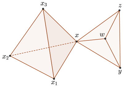
Figure 1. The boundary of a tetrahedron attached to a union of three triangles.

Now we consider the case that $G$ has more than one properly connected component.

Theorem 7.5.

Let $G$ be an $m$-uniform hypergraph with properly connected components. If $c$ is the number of components and $j(I(G))$ is not zero, then

$$j(I(G))=m^{c}e(k[G]).$$

Proof.

Let $G_{1},\ldots,G_{c}$ denote the connected components of $G$. Then by Proposition 5.3 and Theorem 7.2 we obtain $j(I(G))=m^{c}e(k[G_{1}])\cdots e(k[G_{c}])$. Therefore, the result follows from the main theorem of [North] which implies $e(k[G_{1}])\cdots e(k[G_{c}])=e(k[G])$ since $k[G_{1}]\otimes_{k}\cdots\otimes_{k}k[G_{c}]\simeq k[G]$. ∎

Below we also sketch a direct proof of Theorem 7.5 without using the multiplicativity formula in Proposition 5.3 and the main result of [North].

Proof.

Let $\cal G$ be the associated graded ring of $R$ with respect to the edge ideal $I$ of $G$. Then, as in the proof of Theorem 7.2,

$$j(I)=\lambda(\cal G_{{\mathfrak{m}}\cal G})\cdot e(k[G]).$$

We need to show that $\cal G_{{\mathfrak{m}}\cal G}$ has length $m^{c}$. Recall that $\cal G=\cal R/I\cal R$, where $\cal R$ is the Rees algebra of $I$. Thus $\cal G_{{\mathfrak{m}}\cal G}\simeq\cal R_{\,{\mathfrak{m}}\cal R}/I\cal R_{\,{\mathfrak{m}}\cal R}$. Now let $X_{k}\subset\{x_{1},\dots,x_{n}\}$ be the set of the nodes of the connected component $G_{k}$, so $\{x_{1},\dots,x_{n}\}$ is the disjoint union of $X_{1},\dots,X_{c}$. After a possible relabeling of the nodes we may assume that $x_{k}\in X_{k}$ for $k=1,\ldots,c$. Then Lemma 7.3 implies $(X_{k})\cal R_{\,{\mathfrak{m}}\cal R}=(x_{k})\cal R_{\,{\mathfrak{m}}\cal R}$ for $k=1,\ldots,c$. Therefore,

$${\mathfrak{m}}\cal G_{{\mathfrak{m}}\cal G}=(x_{1},\ldots,x_{c})\cal G_{{\mathfrak{m}}\cal G}.$$

Also $(x_{k}^{m})\cal G_{{\mathfrak{m}}\cal G}=(0)$ for all $k=1,\ldots,c$ as in the proof of Theorem 7.2. Thus, by the pigeonhole principle

$${\mathfrak{m}}^{c(m-1)+1}\cal G_{{\mathfrak{m}}\cal G}=(0).$$

Furthermore, it can be readily seen that for $i=0,\ldots,c(m-1)$ the ideal ${\mathfrak{m}}^{i}\cal G_{{\mathfrak{m}}\cal G}$ is minimally generated by monomials $x_{1}^{a_{1}}\cdots x_{c}^{a_{c}}$ of degree $i$ such that the $a_{k}$ are less than $m$. Therefore

$$\lambda(\cal G_{{\mathfrak{m}}\cal G})=\sum_{i=0}^{c(m-1)}\lambda({\mathfrak{m}}^{i}\cal G_{{\mathfrak{m}}\cal G}/{\mathfrak{m}}^{i+1}\cal G_{{\mathfrak{m}}\cal G})$$

is the number of all monomials $x_{1}^{a_{1}}\cdots x_{c}^{a_{c}}$ such that the $a_{k}$ are less than $m$, which is $m^{c}$. ∎

Example 7.6.

Let $G$ be the complete multipartite graph on $n$ nodes of type $(q_{1},\ldots,q_{k})$. If $k$ is at least 3, then by [Hibi, Corollary 2.7] and Theorem 7.2 we obtain

$$j(I(G))=2e(k[G])=2^{n}-2\sum_{i=1}^{k}\sum_{j=1}^{q_{i}}{n-1\choose j-1}.$$

The following result is an immediate consequence of Theorem 7.5 and Corollary 5.1

Corollary 7.7.

Let $G$ be an $m$-uniform hypergraph on $n$ nodes with properly connected components. If $G$ has $c$ connected components and ${\rm Vol}_{n-1}(F(G))\not=0$, equivalently, if the nodes in each connected component of $G$ are pivot equivalent, then

$$e(k[G])=m^{c-1}{\rm Vol}_{n-1}(F(G)).$$

Remark 7.8.

Note that in Theorem 7.2, if we do not assume $G$ is properly connected then the statement fails, as the following example illustrates. Here $G$ is a connected $3$-uniform hypergraph with $V(G)=\{x_{1},x_{2},x_{3},x_{4},x_{5},y_{1},y_{2},y_{3}\}$. The edge set $E(G)$ is given by the triangles in the simplicial complex represented in Figure 2.

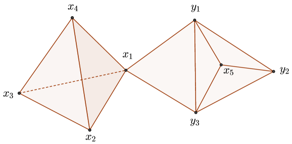
Figure 2. The boundary of a tetrahedron attached to a union of four triangles.

Note that $G$ has 8 nodes and 8 edges, and the incidence matrix $M(G)$ is a square $8\times 8$ matrix of full rank. A simple calculation provides

$$j(G)={\rm Vol}_{8}({\rm pyr}(F(G)))=\det M(G)=6.$$

On the other hand, as in the proof of Proposition 8.2, one can see that the edge ring $k[G]$ is isomorphic to a polynomial ring over a field, and so $e(k[G])=1$, which shows that Theorem 7.2 fails for not properly connected hypergraphs. We can also calculate $j(G)$ directly as in the proof of Theorem 7.2. Recall that

$$j(G)=e(\Gamma_{{\mathfrak{m}}}(\cal G))=\lambda(\cal G_{{\mathfrak{m}}\cal G})\cdot e(k[G])=\lambda(\cal G_{{\mathfrak{m}}\cal G}).$$

Let us show that the length of $\cal G_{{\mathfrak{m}}\cal G}\simeq\cal R_{\,{\mathfrak{m}}\cal R}/I\cal R_{\,{\mathfrak{m}}\cal R}$ is 6. First, note that $G$ has two pivot classes $\{x_{1},x_{2},x_{3},x_{4},x_{5}\}$ and $\{y_{1},y_{2},y_{3}\}$. Then by Lemma 7.3 we have $(x_{i})\cal R_{\,{\mathfrak{m}}\cal R}=(x_{1})\cal R_{\,{\mathfrak{m}}\cal R}$ for $i=1,\ldots 5$, and $(y_{j})\cal R_{\,{\mathfrak{m}}\cal R}=(y_{1})\cal R_{\,{\mathfrak{m}}\cal R}$ for $j=1,2,3$. Thus ${\mathfrak{m}}\cal R_{\,{\mathfrak{m}}\cal R}=(x_{1},y_{1})\cal R_{\,{\mathfrak{m}}\cal R}$. Using edges $\{x_{1},y_{1},y_{3}\}$ and $\{x_{1},x_{2},x_{4}\}$ we have $x_{2}x_{4}(x_{1}y_{1}y_{3}t)=y_{1}y_{3}(x_{1}x_{2}x_{4}t)$. Hence we may write

$$(x_{1}^{2})\cal R_{\,{\mathfrak{m}}\cal R}=(x_{2}x_{4})\cal R_{\,{\mathfrak{m}}\cal R}=(y_{1}y_{3})\cal R_{\,{\mathfrak{m}}\cal R}=(y_{1}^{2})\cal R_{\,{\mathfrak{m}}\cal R}.$$

This implies that ${\mathfrak{m}}^{2}\cal R_{\,{\mathfrak{m}}\cal R}=(x_{1}^{2},x_{1}y_{1})\cal R_{\,{\mathfrak{m}}\cal R}$, ${\mathfrak{m}}^{3}\cal R_{\,{\mathfrak{m}}\cal R}=(x_{1}^{3},y_{1}^{3})\cal R_{\,{\mathfrak{m}}\cal R}$ and ${\mathfrak{m}}^{4}\cal R_{\,{\mathfrak{m}}\cal R}=(x_{1}^{4},x_{1}^{3}y_{1})\cal R_{\,{\mathfrak{m}}\cal R}$. Note that $(x_{1}^{3})\cal R_{\,{\mathfrak{m}}\cal R}=(x_{1}x_{2}x_{3})\cal R_{\,{\mathfrak{m}}\cal R}\subset I\cal R_{\,{\mathfrak{m}}\cal R}$. Therefore, ${\mathfrak{m}}^{4}\cal G_{{\mathfrak{m}}\cal G}=(0)$ and ${\mathfrak{m}}^{i}\cal G_{{\mathfrak{m}}\cal G}/{\mathfrak{m}}^{i+1}\cal G_{{\mathfrak{m}}\cal G}$ for $i=0,1,2,3$ have bases $\{1\}$, $\{x_{1},y_{1}\}$, $\{x_{1}^{2},x_{1}y_{1}\}$, and $\{y_{1}^{3}\}$, respectively. Thus,

$$\lambda(\cal G_{{\mathfrak{m}}\cal G})=\sum_{i=0}^{3}\lambda({\mathfrak{m}}^{i}\cal G_{{\mathfrak{m}}\cal G}/{\mathfrak{m}}^{i+1}\cal G_{{\mathfrak{m}}\cal G})=1+2+2+1=6.$$

8. The $j$-multiplicity of edge ideals and toric edge ideals

Let $I(G)$ be the edge ideal of an $m$-uniform hypergraph $G$ on $n$ nodes $x_{1},\ldots,x_{n}$. As we mentioned in the previous section, the associated edge subring $k[G]$ can be regarded as a standard graded algebra over $k$. Therefore, we may define a homogeneous epimorphism of $k$-algebras

$$\phi:S=k[T_{i_{1}\cdots i_{m}}\ |\ \{x_{i_{1}},\ldots,x_{i_{m}}\}\in E(G)]\to k[G],$$

where the $T_{i_{1}\cdots i_{m}}$ are indeterminates over $k$, by assigning $\phi(T_{i_{1}\cdots i_{m}})=x_{i_{1}}\cdots x_{i_{m}}$ for $\{x_{i_{1}},\ldots,x_{i_{m}}\}\in E(G)$. Thus one obtains a homogeneous isomorphism $k[G]\simeq S/I_{G}$, where $I_{G}=\ker(\phi)$ is a homogeneous prime ideal called the toric edge ideal of $G$. Indeed, the ideal $I_{G}$ is generated by binomials, defining an affine toric variety [Strumfels1].

Proposition 8.1.

Let $G$ be an $m$-uniform hypergraph on $n$ nodes with properly connected components. Let $e$ denote the number of edges, $p$ the number of pivot equivalence classes and $c$ the number of connected components of $G$. Then

$${\rm ht}\,I_{G}=e-n+p-c.$$

Proof.

Recall that ${\rm dim}\,k[G]=\ell(I(G))$ by Remark 7.1. Thus, one can compute the height of the toric edge ideal of $G$ as

$${\rm ht}\,I_{G}={\rm dim}\,S-{\rm dim}\,k[G]=e-\ell(I(G)).$$

If all connected components of $G$ are properly connected then $\ell(I(G))=n-p+c$ by Proposition 6.1 and the result follows. ∎

Recall that if $j(I(G))\not=0$, then by Remark 5.2 the number of edges of $G$ is at least the number of nodes of $G$. The following result deals with the extremal case and extends Proposition 5.6 to $m$-uniform hypergraphs.

Proposition 8.2.

Let $G$ be an $m$-uniform hypergraph with properly connected components. Assume the number of edges of $G$ is equal to the number of nodes of $G$. If $G$ has $c$ connected components and $j(I(G))\not=0$, then

$$j(I(G))=m^{c}.$$

Proof.

Since all connected components of $G$ are properly connected and $j(I(G))\not=0$, by Proposition 6.2, each connected component of $G$ admits only one pivot equivalence class. Then by Proposition 8.1 the toric edge ideal $I_{G}$ has height zero. Thus $I_{G}$ is zero. Hence $k[G]$ is isomorphic to a polynomial ring over a field, and thus $e(k[G])=1$. Therefore, by Theorem 7.5 we obtain

$$j(I(G))=m^{c}e(k[G])=m^{c}.$$

∎

Example 8.3.

If $G$ is the complete $(n-1)$-uniform hypergraph on $n$ nodes, then $e=n$. In addition, $G$ is properly connected and has only one pivot equivalence class. Therefore, by Proposition 8.2 we obtain $j(I(G))=n-1$, as in Example 3.3.

Recall that a walk $w$ of length $s$ in a simple graph $G$ is a sequence of edges of the form

$$\{x_{i_{0}},x_{i_{1}}\},\,\{x_{i_{1}},x_{i_{2}}\},\ldots,\{x_{i_{s-1}},x_{i_{s}}\}.$$

A walk $w$ is called closed if the initial and the end nodes $x_{i_{0}},x_{i_{s}}$ are the same. If $w$ is a closed walk of even length $2l$, then we call $w$ a monomial walk and we define

$$T_{w}=T_{i_{0}i_{1}}T_{i_{2}i_{3}}\cdots T_{i_{2l-2}i_{2l-1}}-T_{i_{1}i_{2}}T_{i_{3}i_{4}}\cdots T_{i_{2l-1}i_{2l}}\in S,$$

which belongs to the toric edge ideal $I_{G}$. Indeed, the toric edge ideal $I_{G}$ is generated by binomials of the form $T_{w}$ associated to monomial walks in $G$ [Vill1]. More generally, one may define monomial walks in an $m$-uniform hypergraph $G$ such that the toric edge ideal $I_{G}$ is generated by the associated binomials [Petrovic]. We say a monomial walk $w$ is nontrivial if $T_{w}\not=0$, and minimal if $T_{w}$ is irreducible. For example, if $G$ is unicyclic with an odd cycle, then it does not admit a nontrivial monomial walk, hence $I_{G}$ is zero as we observed in the proof of Proposition 8.2. Two monomial walks $w$ and $w^{\prime}$ are called equivalent if $T_{w}=T_{w^{\prime}}$.

A simple connected graph $G$ is called bicyclic if the number of edges is one more than the number of nodes. For instance, if $G$ is a simple graph obtained by connecting two disjoint cycles with a path, then $G$ is a bicyclic graph known as a bowtie (Figure 3). If $G$ consists of two cycles with a common node, then we regard it as a bowtie graph where the length of the path between the two cycles is zero. The following result computes the $j$-multiplicity of the edge ideals of bicyclic graphs.

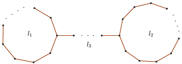
Figure 3. A bicyclic graph of type 1.

Proposition 8.4.

Let $G$ be an $m$-uniform hypergraph with properly connected components. Assume the number of edges in $G$ is one more than the number of nodes and $G$ has $c$ connected components. If $j(I(G))\not=0$, then there is a unique nontrivial minimal monomial walk $w$ in $G$ up to equivalence. Furthermore, if the length of $w$ is $2l$, then

$$j(I(G))=m^{c}l.$$

In particular, if $G$ is a bicyclic graph with an odd cycle, then $j(I(G))$ is the length of the unique nontrivial minimal monomial walk in $G$.

Proof.

Recall that by Proposition 6.2 $j(I(G))\not=0$ if and only if each connected component of $G$ contains only one pivot equivalence class. Then we have ${\rm ht}\,I_{G}=e-n+p-c=1$ by Proposition 8.1. Therefore, $I_{G}$ is a principal prime ideal generated by an irreducible homogeneous binomial $T_{w}$ corresponding to a unique minimal monomial walk $w$ in $G$ up to equivalence. Hence, we obtain $e(k[G])=e(S/I_{G})=e(S/(T_{w}))=\deg T_{w}$. Thus, by Theorem 7.5 we conclude that

$$j(I(G))=m^{c}\cdot e(k[G])=m^{c}\cdot\deg T_{w}.$$

Thus the result follows as the degree of $T_{w}$ is half the length of the monomial walk $w$. ∎

Example 8.5.

Let $G$ be a bicyclic graph, consisting of two cycles of lengths $l_{1}$ and $l_{2}$ connected by a path (Figure 3) or attached along a path of length $l_{3}$ (Figure 4). If both $l_{1}$ and $l_{2}$ are odd, then the length of the unique nontrivial minimal monomial walk in $G$ is $l_{1}+l_{2}+2l_{3}$ for the first type of graphs, and it is $l_{1}+l_{2}-2l_{3}$ for the second type of graphs. Thus,

$$j(I(G))=l_{1}+l_{2}\pm 2l_{3}.$$

If $l_{1}$ is odd and $l_{2}$ is even, then $j(I(G))=l_{2}$, and if both $l_{1}$ and $l_{2}$ are even, then $j(I(G))=0$ by Proposition 5.5.

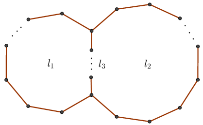
Figure 4. A bicyclic graph of type 2.

One may also obtain the following result as an immediate corollary of Proposition 8.4, Proposition 8.2 and Proposition 5.3.

Corollary 8.6.

Let $G$ be a simple graph in which the connected components are unicyclic or bicyclic. If $j(I(G))$ is not zero, then

$$j(I(G))=2^{c}l_{1}\cdots l_{k},$$

where $c$ is the number of connected components of $G$ and the $l_{i}$ are half the length of the unique nontrivial minimal monomial walks in the bicyclic connected components of $G$.

Remark 8.7.

Note that the toric edge ideal of the graphs as in the statement of the Corollary 8.6 are complete intersections. Let $G$ be an arbirtrary $m$-uniform hypergraph with complete intersection toric edge ideal $I_{G}$, generated by a regular sequence of binomials $T_{w_{1}},\ldots,T_{w_{s}}$. Then

$$e(k[G])=e(S/(T_{w_{1}},\ldots,T_{w_{s}}))=\deg T_{w_{1}}\cdots\deg T_{w_{s}}.$$

Therefore, if $G$ has properly connected components and the $j$-multiplicity of the edge ideal of $G$ is not zero, then by Theorem 7.5 we obtain

$$j(I(G))=m^{c}\cdot e(k[G])=m^{c}\deg T_{w_{1}}\cdots\deg T_{w_{s}}=m^{c}l_{1}\cdots l_{s},$$

where $l_{i}$ is half the length of the monomial walk $w_{i}$ for $i=1,\ldots,s$. In particular, we recover Corollary 8.6 without using Proposition 5.3 and the volumes. For a study of simple graphs with complete intersection toric edge ideals, see [BGR, GRV, TT].

9. Inequalities on the $j$-multiplicity of edge ideals

In this section, we explore the relations between the $j$-multiplicity of the edge ideals of hypergraphs and their subhypergraphs and we obtain general bounds for the $j$-multiplicity of edge ideals. Let $G$ and $H$ be hypergraphs. Then $H$ is called a subhypergraph of $G$ if $V(H)$ and $E(H)$ are subsets of $V(G)$ and $E(G)$, respectively. In Theorem 9.2 below we prove a monotonicity property of the $j$-multiplicity, which will be useful in providing bounds for the $j$-multiplicity of edge ideals. We start with the following geometric observation.

Lemma 9.1.

Let $A$ be any finite set of lattice points in ${\mathbb{R}}^{n}$ and $B\subset A$. Then the normalized volume of ${\rm conv}(B)$ in the affine span of $B$ is no greater than the normalized volume of ${\rm conv}(A)$ in the affine span of $A$.

Proof.

By induction, it is enough to assume that $|A|-|B|=1$. Also, by choosing coordinates we may assume that the affine span of $A$ is ${\mathbb{R}}^{n}$. Let $A\setminus B=\{a\}$. If the affine span of $B$ is also ${\mathbb{R}}^{n}$ then, clearly

$${\rm Vol}_{n}({\rm conv}(B))\leq{\rm Vol}_{n}({\rm conv}(A)).$$

Otherwise, the affine span of $B$ is an affine hyperplane $L\subset{\mathbb{R}}^{n}$ and ${\rm conv}(A)$ is the pyramid over ${\rm conv}(B)$ with apex $a$. Then

$${\rm Vol}_{n-1}({\rm conv}(B))\leq{\rm Vol}_{n}({\rm conv}(A))$$

follows from (2) since the lattice distance from the affine span of $B$ to $a$ is a positive integer. ∎

Theorem 9.2.

Let $G$ be an $m$-uniform hypergraph. If $j(I(G))$ is not zero and $H$ is a subhypergraph of $G$, then

$$j(I(H))\leq j(I(G)).$$

Proof.

Let $A\subset{\mathbb{R}}^{n}$ consist of the origin and the lattice points corresponding to the edges of $G$. Then $j(I(G))={\rm Vol}_{n}({\rm conv}(A))$ by Theorem 3.1. The set of nodes $V(H)$ defines a coordinate subspace of ${\mathbb{R}}^{n}$ which we identify with ${\mathbb{R}}^{k}$, where $k=|V(H)|$. Similarly, let $B\subset{\mathbb{R}}^{k}$ consist of the origin and the lattice points corresponding to the edges of $H$, and, hence, $j(I(H))={\rm Vol}_{k}({\rm conv}(B))$. If the affine span of $B$ equals ${\mathbb{R}}^{k}$ then $j(I(H))\leq j(I(G))$ by Lemma 9.1. Otherwise, $j(I(H))=0$ and the inequality obviously holds. ∎

Remark 9.3.

The above argument easily carries over to the case of arbitrary monomial ideals $I$ in $R=k[x_{1},\dots,x_{n}]_{(x_{1},\dots,x_{n})}$ whose minimal monomial generators have exponents lying in a hyperplane (that is when ${\rm dim}\,F(I)<n$). Namely, if $\cal B$ is a subset of the set of the minimal monomial generators of $I$ and $X\subset\{x_{1},\dots,x_{n}\}$ is the set of variables appearing in $\cal B$ then the ideal $J\subset k[X]_{(X)}$ generated by $\cal B$ satisfies $j(J)\leq j(I)$. Note that the condition ${\rm dim}\,F(I)<n$ is essential here as the following simple example shows. If $I=\langle x^{3},xy,y^{3}\rangle$ and $J=\langle x^{3},y^{3}\rangle$ in $R=k[x,y]_{(x,y)}$ then $j(J)>j(I)$.

Corollary 9.4.

Let $G$ be an $m$-uniform hypergraph on $n$ nodes. Then $j(I(G))$ is bounded above by the $j$-multiplicity of the edge ideal of the complete $m$-uniform hypergraph on $n$ nodes mentioned in Example 3.3. In particular if $G$ is a simple graph, then $j(I(G))$ is at most $2^{n}-2n$.

Let $G$ be a simple graph with odd tulgeity $\tau_{0}$, which is the maximum number of node-disjoint odd cycles in $G$. Let $H$ be a subgraph of $G$ consisting of $\tau_{0}$ node-disjoint odd cycles in $G$. Then by Proposition 5.6 or Proposition 8.2, the $j$-multiplicity of $I(H)$ is $2^{\tau_{0}}$. Therefore, if $I(G)$ has nonzero $j$-multiplicity, then $j(I(G))\geq 2^{\tau_{0}}$ by Theorem 9.2. On the other hand, if $G$ is a multipartite graph of type $(q_{1},\ldots,q_{k})$, then by Theorem 9.2 $j(I(G))$ is bounded above by the $j$-multiplicity of the complete multipartite graph of type $(q_{1},\ldots,q_{k})$ as in Example 7.6. Therefore, we obtain the following corollary.

Corollary 9.5.

Let $G$ be a simple multipartite graph of type $(q_{1},\ldots,q_{k})$ with $n$ nodes and odd tulgeity $\tau_{0}$. If the $j$-multiplicity of $I(G)$ is not zero, then

$$2^{\tau_{0}}\leq j(I(G))\leq 2^{n}-2\sum_{i=1}^{k}\sum_{j=1}^{q_{i}}{n-1\choose j-1}.$$

For a node $x$ in $G$, we let $G-x$ denote the subhypergraph of $G$ obtained by removing $x$ and the edges containing it from $G$. We say that $x$ is a free node if it is contained in only one edge in $E(G)$. For simple graphs a free node is also known as a whisker. Recall that by Theorem 9.2, $j(I(G-x))\leq j(I(G))$ for any node $x$ in $G$. Below we note that equality holds for free nodes.

Proposition 9.6.

Let $G$ be an $m$-uniform hypergraph containing a free node $x$. Then

$$j(I(G))=j(I(G-x)).$$

Proof.

If $x_{i}\in V(G)=\{x_{1},\ldots,x_{n}\}$ is a free node, then removing $x_{i}$ and the corresponding edge from $G$ is equivalent to removing the unique vertex of the edge polytope $F(G)$ with $z_{i}$-coordinate being $1$. Note that $F(G)$ is a pyramid with apex at this vertex and base $F(G-x_{i})$. Since the base lies in the hyperplane $z_{i}=0$, the height of the pyramid is one. Therefore the normalized $(n-1)$-volume of $F(G)$ equals the normalized $(n-2)$-volume of the base $F(G-x_{i})$. Then by Corollary 5.1 we obtain

$$j(I(G))=m\cdot{\rm Vol}_{n-1}(F(G))=m\cdot{\rm Vol}_{n-2}(F(G-x_{i}))=j(I(G-x_{i})).$$

∎

One could also prove Proposition 9.6 algebraically for simple graphs using toric edge ideals as follows.

Proof.

By Proposition 5.3 we may assume $G$ is connected. We may further assume $G$ contains an odd cycle, otherwise the statement is trivilally true as both $j(I(G))$ and $j(I(G-x))$ are zero. Let $\alpha$ be the only edge in $E(G)$ containing $x$. Then $\alpha$ is not part of any nontrivial minimal monomial walk in $G$. Therefore, if we write $k[G]\simeq S/I_{G}$ as in Section 8, then $\alpha$ corresponds to a variable $T_{\alpha}$ in $S$ not appearing in the generators of the toric edge ideal $I_{G}$. If we let $\bar{S}=S/(T_{\alpha})$ and consider $\alpha$ as an element in $k[G]$, then we have the following homogenous isomorphisms of graded $k$-algebras,

$$k[G]/(\alpha)\simeq S/(I_{G}+(T_{\alpha}))\simeq\bar{S}/I_{G-x}\simeq k[G-x].$$

Therefore, using the homogenous short exact sequence

$$0\rightarrow k[G](-1)\xrightarrow{\alpha}k[G]\rightarrow k[G]/(\alpha)\simeq k[G-x]\rightarrow 0$$

we obtain $e(k[G])=e(k[G-x])$. Now since both $G$ and $G-x$ are connected and contain an odd cycle, by Theorem 7.2 we conclude

$$j(I(G))=2e(k[G])=2e(k[G-x])=j(I(G-x)).$$

∎

The following result gives a lower bound for the $j$-multiplicity of the edge ideal of an $m$-uniform hypergraph in terms of the multiplicity of the associated edge subring.

Proposition 9.7.

Let $G$ be an $m$-uniform hypergraph with $c$ connected components, not necessarily properly connected. If $j(I(G))$ is not zero, then

$$j(I(G))\geq m^{c}\cdot e(k[G]).$$

Proof.

If $G$ is a connected $m$-uniform hypergraph, not necessarily properly connected, then as in the proof of Theorem 7.2 we have

$$j(I(G))=\lambda(\cal G_{{\mathfrak{m}}\cal G})\cdot e(k[G])$$

when $j(I(G))$ is not zero. Note that $I\cal R_{\,{\mathfrak{m}}\cal R}\subset{\mathfrak{m}}^{m}\cal R_{\,{\mathfrak{m}}\cal R}$. Thus ${\mathfrak{m}}^{k}\cal G_{{\mathfrak{m}}\cal G}=({\mathfrak{m}}^{k}+I)\cal R_{\,{\mathfrak{m}}\cal R}/I\cal R_{\,{\mathfrak{m}}\cal R}$ is not zero for $k$ less than $m$. Hence,

$$\lambda(\cal G_{{\mathfrak{m}}\cal G})=\sum_{k\geq 1}\lambda({\mathfrak{m}}^{k-1}\cal G_{{\mathfrak{m}}\cal G}/{\mathfrak{m}}^{k}\cal G_{{\mathfrak{m}}\cal G})\geq m.$$

Therefore, $j(I(G))$ is greater than or equal to $m\cdot e(k[G])$. If $G$ is not connected, then the desired inequality follows from Proposition 5.3 and the fact that the multiplicity of the edge subring is multiplicative over the connected components.

∎

Let $G$ be an $m$-uniform hypergraph with properly connected components. Assume the toric edge ideal $I_{G}$ is minimally generated by binomials $T_{w_{1}},\ldots,T_{w_{s}}$. For a description of the minimal generators of the toric edge ideals of simple graphs see [RTT]. Then as in Section 8 we may represent the edge subring $k[G]$ as $S/(T_{w_{1}},\ldots,T_{w_{s}})$. Therefore,

$$e(k[G])=e(S/(T_{w_{1}},\ldots,T_{w_{s}}))\leq\deg T_{w_{1}}\cdots\deg T_{w_{s}}.$$

Hence, by Theorem 7.2 we obtain

$$j(I(G))=m^{c}\cdot e(k[G])\leq m^{c}\deg T_{w_{1}}\cdots\deg T_{w_{s}}.$$

Thus we have the following result.

Proposition 9.8.

Let $G$ be an $m$-uniform hypergraph with properly connected components. Then

$$j(I(G))\leq m^{c}l_{1}\cdots l_{s},$$

where the $l_{i}$ are half the length of the monomial walks in $G$ corresponding to a minimal generating set of $I_{G}$.

Let $G$ be a simple connected graph on $n$ nodes and $e$ edges, such that the edge subring $k[G]$ is Cohen-Macaulay. See for instance [BHO] for a study of graphs with Cohen-Macaulay edge subring. Then Lemma 4.1 in [Hibi2] states that ${\rm Vol}_{n-1}(F(G))$ is at least $e-n+1$ when $G$ is not bipartite. Therefore, by Corollary 5.1 we obtain the following lower bound for the $j$-multiplicity of the edge ideal of $G$.

Proposition 9.9.

Let $G$ be a simple connected graph on $n$ nodes and $e$ edges whose edge subring is Cohen-Macaulay. If $j(I(G))$ is not zero, then

$$j(I(G))\geq 2(e-n+1).$$

10. The $\varepsilon$-multiplicity of edge ideals

We recall the notion of the $\varepsilon$-multiplicity as introduced in [KV] and [UV]. Let $I$ be an arbitrary ideal in a Noetherian local ring $R$ with maximal ideal ${\mathfrak{m}}$ and dimension $n$. Then the $\varepsilon$-multiplicity of $I$ is defined as

$$\varepsilon(I)=n!\limsup_{k}\,\frac{\lambda_{R}(\Gamma_{{\mathfrak{m}}}(R/I^{k}))}{k^{n}}\in{\mathbb{R}}_{\geq 0}.$$

Similar to the $j$-multiplicity, the $\varepsilon$-multiplicity can be viewed as an extension of the Hilbert-Samuel multiplicity to arbitrary ideals, for if $I$ is ${\mathfrak{m}}$-primary, then $\Gamma_{{\mathfrak{m}}}(R/I^{k})=R/I^{k}$, therefore $\varepsilon(I)={e}(I)$. However, the $\varepsilon$-multiplicity exhibits a very different behavior than the $j$-multiplicity. For instance, the $j$-multiplicity is always a non-negative integer, while the $\varepsilon$-multiplicity could be an irrational real number [CHST]. In this section, we will compute the $\varepsilon$-multiplicity of the edge ideal of cycles and complete hypergraphs, which further highlights the differences of the two invariants. The vanishing of the $\varepsilon$-multiplicity of an ideal is captured by the analytic spread of the ideal. Indeed, as in the case of $j$-multiplicity, the $\varepsilon$-multiplicity of $I$ is not zero if and only if the analytic spread of $I$ is maximal [KV, UV]. In particular, by Proposition 6.1 we obtain the following result.

Proposition 10.1.

If $G$ is an $m$-uniform hypergraph with properly connected components, then $\varepsilon(I(G))\not=0$ if and only if the nodes in each connected component of $G$ are pivot equivalent. Recall that for simple graphs, this condition means that each connected component contains an odd cycle.

Let $I$ be a monomial ideal in $R=k[x_{1},\dots,x_{n}]_{(x_{1},\dots,x_{n})}$. Let $L_{i}\subset{\mathbb{R}}^{n}$ be the coordinate hyperplane defined by $z_{i}=0$ and $\pi_{i}:{\mathbb{R}}^{n}\to L_{i}$ the corresponding orthogonal projection. For the Newton polyhedron $P(I)$, define the following

(10) $$\hat{P}(I)=\bigcap_{i=1}^{n}\pi_{i}^{-1}\left(\pi_{i}(P(I))\right),\quad\hat{F}(I)=\operatorname{cl}(\hat{P}(I)\setminus P(I)),$$

where $\operatorname{cl}(K)$ denotes the closure of $K$ in ${\mathbb{R}}^{n}$. The following theorem by Jeffries and Montaño [JM, Theorem 5.1] gives an interpretation of the $\varepsilon$-multiplicity of monomial ideals in terms of the volumes of the associated polytopes.

Theorem 10.2.

Let $I\subset R$ be a monomial ideal. Then $\varepsilon(I)={\rm Vol}_{n}(\hat{F}(I))$.

Note that since $\hat{P}(I)\setminus P(I)$ is bounded, $P(I)$ and $\hat{P}(I)$ coincide outside of a large enough ball. Therefore, $P(I)$ and $\hat{P}(I)$ have the same facet inequalities for their unbounded facets. In particular, since $P(I)=F(I)+{\mathbb{R}}^{n}_{\geq 0}$, the inequalities $z_{i}\geq 0$ for $i=1,\ldots,n$ are among the facet inequalities for both $P(I)$ and $\hat{P}(I)$.

Proposition 10.3.

Let $G_{m,n}$ be the complete $m$-uniform hypergraph on $n$ nodes. Then

$$\varepsilon(I(G_{m,n}))=\frac{n-m}{n-1}A(n-1,m).$$

In particular, for the complete simple graph $G_{2,n}$ and for the complete $(n-1)$-uniform hypergraph $G_{n-1,n}$ we obtain

$$\varepsilon(I(G_{2,n}))=\frac{n-2}{n-1}(2^{n-1}-n),\quad\quad\varepsilon(I(G_{n-1,n}))=\frac{1}{n-1}.$$

Proof.

Denote $I_{m,n}=I(G_{m,n})$. Clearly, when $m=n$ we have $I_{n,n}=(x_{1}\cdots x_{n})$ and $\varepsilon(I_{n,n})=0$ which agrees with the formula in the statement. Thus we may assume that $m>n$. Let $P=P(I_{m,n})$ be the Newton polyhedron of $I_{m,n}$ and $F=F(I_{m,n})$ its compact facet. Recall from Example 3.3 that $F$ is given by $\sum_{j=1}^{n}z_{j}=m$. For every $i=1,\ldots,n$ the projection $\pi_{i}(P)$ equals $P(I_{m-1,n-1})$ embedded in the coordinate hyperplane $z_{i}=0$. This implies that $\pi_{i}^{-1}\pi_{i}(P)$ has a facet given by $\langle u_{i},z\rangle\geq m-1$, where $u_{i}=-e_{i}+\sum_{j=1}^{n}e_{j}$. Therefore, $\hat{P}(I_{m,n})$ is given by the facet inequalities $\langle u_{i},z\rangle\geq m-1$ and $z_{i}\geq 0$ for all $i=1,\ldots,n$. Since these facets are unbounded, they are also the unbounded facets of $P$. This shows that $\hat{F}(I_{m,n})$ is a pyramid over $F$ with apex $a=\big{(}\frac{m-1}{n-1},\dots,\frac{m-1}{n-1}\big{)}$. Consequently, by Example 3.3 and equation (2) we obtain

(11) $$\varepsilon(I_{m,n})={\rm Vol}_{n}(\hat{F}(I_{m,n}))=\Big{(}m-\frac{n(m-1)}{n-1}\Big{)}{\rm Vol}_{n-1}(F)=\frac{n-m}{n-1}A(n-1,m).$$

∎

Proposition 10.4.

Let $G$ be a cycle of length $n$. If $n$ is even, then $\varepsilon(I(G))=0$. If $n$ is odd, then

$$\varepsilon(I(G))=\frac{2}{n+1}.$$

Proof.

If $n$ is even then $\varepsilon(I(G))=0$ by Proposition 10.1, so assume $n=2k+1$ for $k\in{\mathbb{N}}$. To simplify notation we set $P=P(I)$, $F=F(I)$, and let $\hat{P}=\hat{P}(I)$ and $\hat{F}=\hat{F}(I)$ as defined in (10). By Theorem 10.2, $\varepsilon(I(G))={\rm Vol}_{n}(\hat{F})$. In Proposition 10.7 below we show that $\hat{F}$ is the pyramid over $F$ with apex $a=\big{(}\frac{1}{k+1},\dots,\frac{1}{k+1}\big{)}$. Since $F$ lies in the hyperplane $\sum_{j=1}^{n}z_{j}=2$ and ${\rm Vol}_{n-1}(F)=1$ the equation (2) produces

$${\rm Vol}_{n}(\hat{F})=\Big{(}2-\frac{n}{k+1}\Big{)}{\rm Vol}_{n-1}(F)=\frac{2}{n+1}.$$

∎

To show that $\hat{F}$ is a pyramid over $F$ we first describe the facet inequalities of $\hat{P}$ in Lemma 10.5 below. Recall that the circulant matrix $C_{u}$ generated by a vector $u=(u_{0},\dots,u_{n-1})\in{\mathbb{R}}^{n}$ is the $n\times n$ matrix whose rows are obtained by the cyclic permutations of the entries of $u$. The associated polynomial $f_{u}(t)=u_{0}+u_{1}t+\dots+u_{n-1}t^{n-1}$ of $C_{u}$ gives a formula for the rank of $C_{u}$ [Ingleton, Proposition 1.1]:

(12) $$\operatorname{rank}(C_{u})=n-\deg\left(\gcd(t^{n}-1,f_{u}(t))\right).$$

Lemma 10.5.

The facets of $\hat{P}$ are defined by the inequalities $I_{n}\,z\geq 0$, $C_{u}\,z\geq{\bf 1}$, where $I_{n}$ is the identity matrix, ${\bf 1}$ is the vector of 1’s, and $C_{u}$ is the circulant matrix generated by $u=e_{1}+\sum_{i=1}^{k}e_{2i}\in{\mathbb{R}}^{n}$, where $n=2k+1$. The same inequalities define the unbounded facets of $P$.

Proof.

First let us describe the primitive normals to the facets of $F_{i}=\pi_{i}(F)$. By definition, $F$ is an $(n-1)$-simplex lying in the hyperplane $\sum_{j=1}^{n}z_{j}=2$ whose vertices are the rows of the incidence matrix of the cycle $G$. Then $F_{i}$ is an $(n-1)$-simplex lying in $L_{i}$ whose vertices are the rows of the incidence matrix of a “graph” $G_{i}$ which is a cycle with omitted $i$-th node, so the rows corresponding to the edges with a missing node are two standard basis vectors, see Figure 5 for an example.

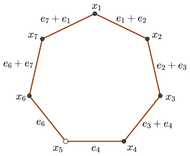
Figure 5. A cycle with an omitted 5-th node.

Since $F_{i}$ is a simplex, for every vertex $v\in F_{i}$ there is exactly one facet $F_{i}(v)$ not containing $v$. Here is a combinatorial way to produce a primitive normal to $F_{i}(v)$. (Note that its $i$-th entry can be arbitrary, so we may assume it is zero. Then it is unique up to sign.) Removing the edge from $G_{i}$ corresponding to $v$, we obtain a “graph” $G_{i}(v)$. Place $0$ and $1$ at the nodes of $G_{i}(v)$ in an alternating way starting with the $0$ in $i$-th node and going both ways. This results in a vector $u(v)\in{\mathbb{R}}^{n}$which is a primitive normal to $F_{i}(v)$. This process is illustrated in Figure 6 with $n=7$, $i=5$, and $v$ corresponding to the edge $\{x_{1},x_{2}\}$.

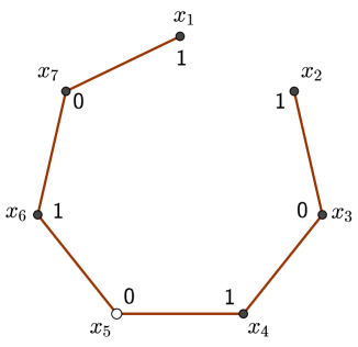
Figure 6. The vector $u(v)=(1,1,0,1,0,1,0)$ is normal to $F_{5}(v)$ for $v=\{x_{1},x_{2}\}$.

Indeed, $u$ is normal to $F_{i}(v)$ if and only if the linear function $\langle u,z\rangle$ takes the same value at all vertices of $F_{i}$, but $v$. Assume for simplicity that $v$ corresponds to $\{x_{1},x_{2}\}$ and $i=n=2k+1$. Then $v=e_{1}+e_{2}$ and the remaining vertices are $e_{2}+e_{3},\dots,e_{2k-1}+e_{2k},e_{2k},e_{1}$. Let $u=(u_{1},\dots,u_{2k+1})$. Then $\langle u,z\rangle$ takes the same value on the remaining vertices if and only if

$$u_{2}+u_{3}=u_{3}+u_{4}=\dots=u_{2k-1}+u_{2k}=u_{2k}=u_{1},$$

which implies $u_{2}=u_{4}=\dots=u_{2k}$ and $u_{3}=u_{5}=\dots=u_{2k-1}$, together with $u_{2k-1}=0$ and $u_{2k}=u_{1}$. Since $u$ is primitive, $u_{1}=u_{2}=u_{4}=\dots=u_{2k}=1$ which justifies the combinatorial process of producing $u(v)$. The general case is similar.

Notice that the value of $\langle u(v),z\rangle$ at all vertices of $F_{i}$, but $v$ equals 1. Furthermore, its value at $v$ equals the sum of the two values placed at the nodes of $v$. These can be either both 1 or both 0. This shows that $u(v)$ is an inner normal to $\pi_{i}^{-1}(F_{i})$ and, hence, to $\pi_{i}^{-1}(\pi_{i}(P))$ if and only if the two values are both 1. Thus, the primitive inner normals to the facets of $\pi_{i}^{-1}(\pi_{i}(P))$ are vectors obtained by a cyclic permutation of $(1,1,0,1,0\dots,1,0)$ and every such vector is the primitive inner normal to a facet of $\pi_{i}^{-1}(\pi_{i}(P))$ for some $i$. Therefore, the facets of $\hat{P}$ are given by $C_{u}\,z\geq{\bf 1}$ for $u=(1,1,0,1,0\dots,1,0)$, as stated.

Finally, we remark that all the facets of $\hat{P}$ are unbounded as the corresponding normals have at least one coordinate equal zero. Thus, the same inequalities describe the unbounded facets of $P$. ∎

Lemma 10.6.

Let $C_{u}$ be the circulant matrix generated by $u=(1,1,0,1,0\dots,1,0)$ in ${\mathbb{R}}^{n}$ for $n=2k+1$. Then $\operatorname{rank}C_{u}=n$.

Proof.

Let $f_{u}(t)=1+t+t^{3}+\dots+t^{2k-1}$ be the associated polynomial and let $g(t)=t^{n}-1$. By (12), $\operatorname{rank}C_{u}=n-\deg\left(\gcd(g(t),f_{u}(t))\right)$. Note that $(t^{2}-1)f_{u}(t)-g(t)=t(t-1)$. But neither $t=0$ nor $t=1$ is a root of $f(t)$, hence $\gcd(g(t),f_{u}(t))=1$ and the statement follows. ∎

Proposition 10.7.

The polytope $\hat{F}$ is the pyramid over $F$ with apex at $a=\big{(}\frac{1}{k+1},\dots,\frac{1}{k+1}\big{)}$.

Proof.

Recall that $F$ is the unique compact facet of $P$ corresponding to the inequality $\sum_{j=1}^{n}z_{j}\geq 2$. Since $\hat{F}=\operatorname{cl}(\hat{P}\setminus P)$ lies in the other half space and the remaining facets inequalities for $\hat{P}$ and $P$ are the same, we conclude that $\hat{F}$ is given by $C_{u}\,z\geq{\bf 1}$ and $\sum_{j=1}^{n}z_{j}\leq 2$. (One can see that the inequalities $I_{n}\,z\geq 0$ are redundant. Indeed, given $1\leq i\leq n$, add the two inequalities in $C_{u}\,z\geq{\bf 1}$ with $1$’s at the $i$-th and at the two adjacent places to obtain $z_{i}+2\geq z_{i}+\sum_{j=1}^{n}z_{j}\geq 2$, which implies $z_{i}\geq 0$.) By Lemma 10.6, $a=\big{(}\frac{1}{k+1},\dots,\frac{1}{k+1}\big{)}$ is the unique solution to $C_{u}\,z={\bf 1}$ which implies that $\hat{F}$ is the pyramid over $F$ with apex $a$.

∎

Remark 10.8.

Unlike the $j$-multiplicity in Proposition 5.3, the $\varepsilon$-multiplicity of edge ideals is not multiplicative over the connected components of a graph. For instance, if $G$ is the disjoint union of a 3-cycle and a 5-cycle, then by direct computation using Theorem 10.2 the $\varepsilon$-multiplicity of the edge ideal of $G$ is $\frac{4}{9}$, while by Proposition 10.4 the $\varepsilon$-multiplicity of the edge ideals of the 3-cycle and the 5-cycle are $\frac{1}{2}$ and $\frac{1}{3}$ respectively. Furthermore, in contrast to Proposition 9.6 for $j$-multiplicity, the $\varepsilon$-multiplicity is not preserved after removal of a free node. For example, if $G$ is a 3-cycle with a path of length 2 attached to one of its nodes, then the $\varepsilon$-multiplicity of $I(G)$ is indeed $\frac{1}{3}$, while after removing the free node the $\varepsilon$-multiplicity of the edge ideal is $\frac{1}{2}$. This example also shows that the $\varepsilon$-multiplicity may increase if we pass to a subgraph. Therefore Theorem 9.2 does not hold true for the $\varepsilon$-multiplicity of edge ideals. However, since the $\varepsilon$-multiplicity is less than or equal to the $j$-multiplicity for an arbitrary ideal [UV], the upper bounds in Corollary 9.4 and Corollary 9.5 are valid for the $\varepsilon$-multiplicity of the edge ideals as well.

References

- [1] AchillesR.ManaresiM.Multiplicity for ideals of maximal analytic spread and intersection theoryJ. Math. Kyoto Univ.33199341029–1046@article{AM, author = {Achilles, R.}, author = {Manaresi, M.}, title = {Multiplicity for ideals of maximal analytic spread and intersection theory}, journal = {J. Math. Kyoto Univ.}, volume = {33}, date = {1993}, number = {4}, pages = {1029–1046}}
- [3] BermejoI.García-MarcoI.ReyesE.Graphs and complete intersection toric idealsJ. Algebra Appl.14201591540011, 37@article{BGR, author = {Bermejo, I.}, author = {Garc{\'{\i}}a-Marco, I.}, author = {Reyes, E.}, title = {Graphs and complete intersection toric ideals}, journal = {J. Algebra Appl.}, volume = {14}, date = {2015}, number = {9}, pages = {1540011, 37}}
- [5] BeyarslanS.HàH. T.O’KeefeA.Cohen-macaulay toric rings associated to graphs arXiv:1703.08270@article{BHO, author = {Beyarslan, S.}, author = {H{\`a}, H. T.}, author = {O'Keefe, A.}, title = { Cohen-Macaulay toric rings associated to graphs}, journal = { arXiv:1703.08270}}
- [7] Bivià-AusinaC.The analytic spread of monomial idealsComm. Algebra31200373487–3496@article{AB, author = {Bivi{\`a}-Ausina, C.}, title = {The analytic spread of monomial ideals}, journal = {Comm. Algebra}, volume = {31}, date = {2003}, number = {7}, pages = {3487–3496}}
- [9] BjörnerA.KarlanderJ.The mod rank of incidence matrices for connected uniform hypergraphsEuropean J. Combin.1419933151–155@article{BK, author = {Bj{\"o}rner, A.}, author = {Karlander, J.}, title = {The mod $p$ rank of incidence matrices for connected uniform hypergraphs}, journal = {European J. Combin.}, volume = {14}, date = {1993}, number = {3}, pages = {151–155}}
- [11] BrunsW.HerzogJ.Cohen-macaulay ringsCambridge Studies in Advanced Mathematics39Cambridge University Press, Cambridge1993@book{BH, author = {Bruns, W.}, author = {Herzog, J.}, title = {Cohen-Macaulay rings}, series = {Cambridge Studies in Advanced Mathematics}, volume = {39}, publisher = {Cambridge University Press, Cambridge}, date = {1993}}
- [13] ChevalleyC.On the theory of local ringsAnn. of Math. (2)441943690–708@article{Chevalley1, author = {Chevalley, C.}, title = {On the theory of local rings}, journal = {Ann. of Math. (2)}, volume = {44}, date = {1943}, pages = {690–708}}
- [15] ChevalleyC.Intersections of algebraic and algebroid varietiesTrans. Amer. Math. Soc.5719451–85@article{Chevalley2, author = {Chevalley, C.}, title = {Intersections of algebraic and algebroid varieties}, journal = {Trans. Amer. Math. Soc.}, volume = {57}, date = {1945}, pages = {1–85}}
- [17] CutkoskyS.HàH. T.SrinivasanH.TheodorescuE.Asymptotic behavior of the length of local cohomologyCanad. J. Math.57200561178–1192@article{CHST, author = {Cutkosky, S.}, author = {H{\`a}, H. T.}, author = {Srinivasan, H.}, author = {Theodorescu, E.}, title = {Asymptotic behavior of the length of local cohomology}, journal = {Canad. J. Math.}, volume = {57}, date = {2005}, number = {6}, pages = {1178–1192}}
- [19] D’AlìA.Toric ideals associated with gap-free graphsJ. Pure Appl. Algebra219201593862–3872@article{DA, author = {D'Al{\`{\i}}, A.}, title = {Toric ideals associated with gap-free graphs}, journal = {J. Pure Appl. Algebra}, volume = {219}, date = {2015}, number = {9}, pages = {3862–3872}}
- [21] FlennerH.ManaresiM.A numerical characterization of reduction idealsMath. Z.23820011205–214@article{FM, author = {Flenner, H.}, author = {Manaresi, M.}, title = {A numerical characterization of reduction ideals}, journal = {Math. Z.}, volume = {238}, date = {2001}, number = {1}, pages = {205–214}}
- [23] FlennerH.O’CarrollL.VogelW.Joins and intersectionsSpringer Monographs in MathematicsSpringer-VerlagBerlin1999vi+307@book{FOV, author = {Flenner, H.}, author = {O'Carroll, L.}, author = {Vogel, W.}, title = {Joins and intersections}, series = {Springer Monographs in Mathematics}, publisher = {Springer-Verlag}, place = {Berlin}, date = {1999}, pages = {vi+307}}
- [25] GawrilowE.JoswigM.Polymake: a framework for analyzing convex polytopes43–74KalaiGilZieglerGünter M.Polytopes — Combinatorics and ComputationBirkhäuser2000@article{polymake, author = {E. Gawrilow and M. Joswig}, title = {polymake: a Framework for Analyzing Convex Polytopes}, pages = {43-74}, editor = {Gil Kalai and G\"unter M. Ziegler}, booktitle = {Polytopes — Combinatorics and Computation}, publisher = {Birkh\"auser}, year = {2000}}
- [27] GitlerI.ValenciaC. E.Multiplicities of edge subringsDiscrete Math.30220051-3107–123@article{GilVal, author = {Gitler, I.}, author = {Valencia, C. E.}, title = {Multiplicities of edge subrings}, journal = {Discrete Math.}, volume = {302}, date = {2005}, number = {1-3}, pages = {107–123}}
- [29] GitlerI.ReyesE.VillarrealR. H.Ring graphs and complete intersection toric idealsDiscrete Math.31020103430–441@article{GRV, author = {Gitler, I.}, author = {Reyes, E.}, author = {Villarreal, R. H.}, title = {Ring graphs and complete intersection toric ideals}, journal = {Discrete Math.}, volume = {310}, date = {2010}, number = {3}, pages = {430–441}}
- [31] GraysonD.StillmanM.Macaulay2, a software system for research in algebraic geometryAvailable at http://www.math.uiuc.edu/Macaulay2/@article{M2, author = {Grayson, D.}, author = {Stillman, M.}, title = {Macaulay2, a software system for research in algebraic geometry}, journal = {Available at \url{http://www.math.uiuc.edu/Macaulay2/}}}
- [33] GrossmanJ. W.KulkarniD. M.SchochetmanI. E.On the minors of an incidence matrix and its smith normal formLinear Algebra Appl.2181995213–224@article{Grossman, author = {Grossman, J. W.}, author = {Kulkarni, D. M.}, author = {Schochetman, I. E.}, title = {On the minors of an incidence matrix and its Smith normal form}, journal = {Linear Algebra Appl.}, volume = {218}, date = {1995}, pages = {213–224}}
- [35] HibiT.OhsugiH.Compressed polytopes, initial ideals and complete multipartite graphsIllinois J. Math.4420002391–406@article{Hibi, author = {Hibi, T.}, author = {Ohsugi, H.}, title = {Compressed polytopes, initial ideals and complete multipartite graphs}, journal = {Illinois J. Math.}, volume = {44}, date = {2000}, number = {2}, pages = {391–406}}
- [37] HibiT.OhsugiH.Toric ideals generated by quadratic binomialsJ. Algebra21819992509–527@article{Hibi2, author = {Hibi, T.}, author = {Ohsugi, H.}, title = {Toric ideals generated by quadratic binomials}, journal = {J. Algebra}, volume = {218}, date = {1999}, number = {2}, pages = {509–527}}
- [39] IngletonA. W.The rank of circulant matricesJ. London Math. Soc.Journal of the London Mathematical Society. Second Series311956632–635ISSN 0024-610715.0X0080623N. G. de BruijnMathReview (N. G. de Bruijn)@article{Ingleton, author = {Ingleton, A. W.}, title = {The rank of circulant matrices}, journal = {J. London Math. Soc.}, fjournal = {Journal of the London Mathematical Society. Second Series}, volume = {31}, year = {1956}, pages = {632–635}, issn = {0024-6107}, mrclass = {15.0X}, mrnumber = {0080623}, mrreviewer = {N. G. de Bruijn}}
- [41] JeffriesJ.MontañoJ.J-multiplicity of monomial idealsMathematical Research Letters2020134729 744@article{JM, author = {Jeffries, J.}, author = {Monta{\~n}o, J.}, title = {j-multiplicity of monomial ideals}, journal = {Mathematical Research Letters}, volume = {20}, date = {2013}, number = {4}, pages = {729 744}}
- [43] JeffriesJ.MontañoJ.VarbaroM.Multiplicities of classical varietiesProc. Lond. Math. Soc. (3)110201541033–1055@article{JMV, author = {Jeffries, J.}, author = {Monta{\~n}o, J.}, author = {Varbaro, M.}, title = {Multiplicities of classical varieties}, journal = {Proc. Lond. Math. Soc. (3)}, volume = {110}, date = {2015}, number = {4}, pages = {1033–1055}}
- [45] KatzD.ValidashtiJ.Multiplicities and rees valuationsCollect. Math.61201011–24@article{KV, author = {Katz, D.}, author = {Validashti, J.}, title = {Multiplicities and Rees valuations}, journal = {Collect. Math.}, volume = {61}, date = {2010}, number = {1}, pages = {1–24}}
- [47] ManteroP.XieY.Generalized stretched ideals and sally’s conjectureJ. Pure Appl. Algebra220201631157–1177@article{MX, author = {Mantero, P.}, author = {Xie, Y.}, title = {Generalized stretched ideals and Sally's conjecture}, journal = {J. Pure Appl. Algebra}, volume = {220}, date = {2016}, number = {3}, pages = {1157–1177}}
- [49] MoreyS.VillarrealR. H.Edge ideals: algebraic and combinatorial propertiestitle={Progress in commutative algebra 1}, publisher={de Gruyter, Berlin}, 201285–126@article{MV, author = {Morey, S.}, author = {Villarreal, R. H.}, title = {Edge ideals: algebraic and combinatorial properties}, conference = {title={Progress in commutative algebra 1}, }, book = {publisher={de Gruyter, Berlin}, }, date = {2012}, pages = {85–126}}
- [51] NishidaK.UlrichB.Computing -multiplicitiesJ. Pure Appl. Algebra2142010122101–2110@article{NU, author = {Nishida, K.}, author = {Ulrich, B.}, title = {Computing $j$-multiplicities}, journal = {J. Pure Appl. Algebra}, volume = {214}, date = {2010}, number = {12}, pages = {2101–2110}}
- [53] NorthcottD. G.The hilbert function of the tensor product of two multigraded modulesMathematika10196343–57@article{North, author = {Northcott, D. G.}, title = {The Hilbert function of the tensor product of two multigraded modules}, journal = {Mathematika}, volume = {10}, date = {1963}, pages = {43–57}}
- [55] OhsugiH.HibiT.Normal polytopes arising from finite graphsJ. AlgebraJournal of Algebra20719982409–426@article{OH1998, author = {Ohsugi, H.}, author = {Hibi, T.}, title = {Normal polytopes arising from finite graphs}, journal = {J. Algebra}, fjournal = {Journal of Algebra}, volume = {207}, year = {1998}, number = {2}, pages = {409–426}}
- [57] PetrovićS.StasiD.Toric algebra of hypergraphsJ. Algebraic Combin.3920141187–208@article{Petrovic, author = {Petrovi{\'c}, S.}, author = {Stasi, D.}, title = {Toric algebra of hypergraphs}, journal = {J. Algebraic Combin.}, volume = {39}, date = {2014}, number = {1}, pages = {187–208}}
- [59] PoliniC.XieY.-Multiplicity and depth of associated graded modulesJ. Algebra379201331–49@article{PX, author = {Polini, C.}, author = {Xie, Y.}, title = {$j$-multiplicity and depth of associated graded modules}, journal = {J. Algebra}, volume = {379}, date = {2013}, pages = {31–49}}
- [61] ReesD.-Transforms of local rings and a theorem on multiplicities of idealsProc. Cambridge Philos. Soc.5719618–17@article{R1, author = {Rees, D.}, title = {${\germ a}$-transforms of local rings and a theorem on multiplicities of ideals}, journal = {Proc. Cambridge Philos. Soc.}, volume = {57}, date = {1961}, pages = {8–17}}
- [63] ReyesE.TatakisC.ThomaA.Minimal generators of toric ideals of graphsAdv. in Appl. Math.482012164–78@article{RTT, author = {Reyes, E.}, author = {Tatakis, C.}, author = {Thoma, A.}, title = {Minimal generators of toric ideals of graphs}, journal = {Adv. in Appl. Math.}, volume = {48}, date = {2012}, number = {1}, pages = {64–78}}
- [65] RyaboginD.ZvavitchA.Analytic methods in convex geometryAnalytical and probabilistic methods in the geometry of convex bodiesIMPAN Lect. Notes287–183Polish Acad. Sci. Inst. Math., Warsaw2014@book{RyaZva, author = {Ryabogin, D.}, author = {Zvavitch, A.}, title = {Analytic methods in convex geometry}, booktitle = {Analytical and probabilistic methods in the geometry of convex bodies}, series = {IMPAN Lect. Notes}, volume = {2}, pages = {87–183}, publisher = {Polish Acad. Sci. Inst. Math., Warsaw}, year = {2014}}
- [67] SamuelP.La notion de multiplicité en algèbre et en géométrie algébriqueFrenchJ. Math. Pures Appl. (9)301951159–274@article{Samuel1, author = {Samuel, P.}, title = {La notion de multiplicit\'e en alg\`ebre et en g\'eom\'etrie alg\'ebrique}, language = {French}, journal = {J. Math. Pures Appl. (9)}, volume = {30}, date = {1951}, pages = {159–274 }}
- [69] SamuelP.Algèbre localeFrenchMémor. Sci. Math., no. 123Gauthier-Villars, Paris195376@book{Samuel2, author = {Samuel, P.}, title = {Alg\`ebre locale}, language = {French}, series = {M\'emor. Sci. Math., no. 123}, publisher = {Gauthier-Villars, Paris}, date = {1953}, pages = {76}}
- [71] SimisA.VasconcelosW. V.VillarrealR. H.On the ideal theory of graphsJ. Algebra16719942389–416@article{SVV, author = {Simis, A.}, author = {Vasconcelos, W. V.}, author = {Villarreal, R. H.}, title = {On the ideal theory of graphs}, journal = {J. Algebra}, volume = {167}, date = {1994}, number = {2}, pages = {389–416}}
- [73] SturmfelsB.Gröbner bases and convex polytopesUniversity Lecture Series8American Mathematical Society, Providence, RI1996@book{Strumfels1, author = {Sturmfels, B.}, title = {Gr\"obner bases and convex polytopes}, series = {University Lecture Series}, volume = {8}, publisher = {American Mathematical Society, Providence, RI}, date = {1996}}
- [75] TatakisC.ThomaA.On complete intersection toric ideals of graphsJ. Algebraic Combin.3820132351–370@article{TT, author = {Tatakis, C.}, author = {Thoma, A.}, title = {On complete intersection toric ideals of graphs}, journal = {J. Algebraic Combin.}, volume = {38}, date = {2013}, number = {2}, pages = {351–370}}
- [77] TeissierB.Monômes, volumes et multiplicitéstitle={Introduction \`a la th\'eorie des singularit\'es, II}, series={Travaux en Cours}, volume={37}, publisher={Hermann, Paris}, 1988127–141@article{Tei, author = {Teissier, B.}, title = {Mon\^omes, volumes et multiplicit\'es}, conference = {title={Introduction \`a la th\'eorie des singularit\'es, II}, }, book = {series={Travaux en Cours}, volume={37}, publisher={Hermann, Paris}, }, date = {1988}, pages = {127–141}}
- [79] TranTuanZieglerGünter M.Extremal edge polytopesElectron. J. Combin.Electronic Journal of Combinatorics2120142Paper 2.57, 16@article{Ziegler, author = {Tran, Tuan}, author = {Ziegler, G\"unter M.}, title = {Extremal edge polytopes}, journal = {Electron. J. Combin.}, fjournal = {Electronic Journal of Combinatorics}, volume = {21}, year = {2014}, number = {2}, pages = {Paper 2.57, 16}}
- [81] UlrichB.ValidashtiJ.Numerical criteria for integral dependenceMath. Proc. Cambridge Philos. Soc.1512011195–102@article{UV, author = {Ulrich, B.}, author = {Validashti, J.}, title = {Numerical criteria for integral dependence}, journal = {Math. Proc. Cambridge Philos. Soc.}, volume = {151}, date = {2011}, number = {1}, pages = {95–102}}
- [83] VillarrealR. H.Cohen-macaulay graphsManuscripta Math.6619903277–293@article{Vill2, author = {Villarreal, R. H.}, title = {Cohen-Macaulay graphs}, journal = {Manuscripta Math.}, volume = {66}, date = {1990}, number = {3}, pages = {277–293}}
- [85] VillarrealR. H.Rees algebras of edge idealsComm. Algebra23199593513–3524@article{Vill1, author = {Villarreal, R. H.}, title = {Rees algebras of edge ideals}, journal = {Comm. Algebra}, volume = {23}, date = {1995}, number = {9}, pages = {3513–3524}}
- [87] VillarrealR. H.On the equations of the edge cone of a graph and some applicationsManuscripta Math.Manuscripta Mathematica9719983309–317@article{V1998, author = {Villarreal, R. H.}, title = {On the equations of the edge cone of a graph and some applications}, journal = {Manuscripta Math.}, fjournal = {Manuscripta Mathematica}, volume = {97}, year = {1998}, number = {3}, pages = {309–317}}
- [89]