Perspectives on Kuperberg flows

Abstract.

The “Seifert Conjecture” asks, “Does every non-singular vector field on the 3-sphere ${\mathbb{S}}^{3}$ have a periodic orbit?” In a celebrated work, Krystyna Kuperberg gave a construction of a smooth aperiodic vector field on a plug, which is then used to construct counter-examples to the Seifert Conjecture for smooth flows on the $3$-sphere, and on compact 3-manifolds in general. The dynamics of the flows in these plugs have been extensively studied, with more precise results known in special “generic” cases of the construction. Moreover, the dynamical properties of smooth perturbations of Kuperberg’s construction have been considered. In this work, we recall some of the results obtained to date for the Kuperberg flows and their perturbations. Then the main point of this work is to focus attention on how the known results for Kuperberg flows depend on the assumptions imposed on the flows, and to discuss some of the many interesting questions and problems that remain open about their dynamical and ergodic properties.

1. Introduction

The “Seifert Conjecture”, as originally formulated in 1950 by Seifert [43], asked: “Does every non-singular vector field on the $3$-sphere ${\mathbb{S}}^{3}$ have a periodic orbit?” This problem became more specific following the construction in 1966 by F.W. Wilson [48] of a smooth flow on a plug with exactly two periodic orbits. (See also the later paper with Percel [38].) These Wilson plugs could then be used to modify any given flow on a $3$-manifold to obtain one with only isolated periodic orbits. Thus, the Seifert Conjecture is reduced to showing that a flow on a $3$-manifold with only a finite number of periodic orbits can be perturbed to one with no periodic orbits.

Paul Schweitzer showed in the 1974 work [42] how to modify the construction of the Wilson plug in several fundamental ways, to obtain a $C^{1}$-flow with no periodic orbits in the plug. (See also Rosenberg’s survey [41].) He then used this plug to show that for any closed $3$-manifold $M$, there exists a non-singular $C^{1}$-vector field on $M$ without periodic orbits. Jenny Harrison constructed in [20] a modified version of the Schweitzer construction, which she used to construct an aperiodic plug with a $C^{2}$-flow. Finally, in 1994 Krystyna Kuperberg constructed in [28] counter-examples to the smooth version of the Seifert Conjecture.

THEOREM 1.1 (Kuperberg).

On every closed oriented 3-manifold $M$, there exists a $C^{\infty}$ non-vanishing vector field without periodic orbits.

The fascination with this result has many sources. The proof itself introduced a construction of aperiodic$3$-dimensional plugs which was notable for its simplicity and beauty. The Kuperberg construction remains the only general method to date to construct $C^{\infty}$-flows without periodic orbits on arbitrary closed 3-manifolds. The introductory comments in the Séminaire Bourbaki article by Ghys [17] discusses the background and obstacles to the construction of aperiodic flows. Kuperberg has given a brief introduction to the use of plugs in her proof of this result here [31].

The dynamical properties of the Kuperberg flows in these plugs also have many special qualities. The flows must have zero topological entropy, which follows by an observation of Ghys in [17] that an aperiodic flow on a 3-manifold has topological entropy equal to zero, that is a consequence of a well-known result of Katok in [25]. The aperiodic flows in the Kuperberg plugs have a unique minimal set, whose structure is unknown in general, and moreover the generic Kuperberg flow preserves a $2$-dimensional compact lamination with boundary that is contained in the interior of the plug, and contains the minimal set. Finally, the Kuperberg flows have an open set of non-recurrent points that limit on the minimal set, by a result of Matsumoto [34], which adds more to the complexity of the dynamical properties of these flows.

There followed after Kuperberg’s seminal work, a collection of works explaining in further detail the proof of the aperiodicity for the Kuperberg flow in a plug, and investigated its dynamical properties:

• the Séminaire Bourbaki lecture [17] by Étienne Ghys;

• the notes by Shigenori Matsumoto [34] in Japanese, later translated into English;

• the joint paper [29] by Greg Kuperberg and Krystyna Kuperberg;

• the monograph [22] by the authors.

Moreover, a notable feature about the construction of these plugs, is that there are many choices in their construction, which influence the global dynamics of the resulting flows. As Ghys wrote in [17, page 302]:

Par ailleurs, on peut construire beaucoup de pièges de Kuperberg et il n’est pas clair qu’ils aient le même dynamique.

The works cited above suggest many interesting open problems concerning the dynamics of Kuperberg flows. Also, the dynamical properties of flows constructed by variants of the Kuperberg construction which are not aperiodic are studied in [23], showing that the Kuperberg flows are indeed very special, as they lie at the “boundary of chaos” in the $C^{\infty}$-topology on flows.

The purpose of this paper is to collect together these open problems, as well as to formulate more precisely further questions about Kuperberg flows which have arisen in their study, to illuminate the surprising dynamical complexities of the flows that can arise in this very special class of examples.

We first describe the construction of the Kuperberg plugs in Sections 2 and 3, with an emphasis on the choices involved. Section 2 gives the construction of the modified Wilson plugs, which are the foundation of the construction. Section 3 gives the construction of the Kuperberg plugs. These constructions are given in a succinct manner, and the interested reader should consult the literature cited above for further details and discussions.

Section 4 introduces the additional assumptions imposed on the constructions of Kuperberg flows in the works [22, 23], which are called the generic hypotheses. We also introduce variations of these generic hypotheses, whose implications for the dynamics of the flows will be discussed in later sections.

It was observed in the works [17, 34] that any orbit not escaping the plug in forward or backward time, limits to the invariant set defined as the closure of the “special orbits” for the flow. One consequence is that the Kuperberg flow in a plug has a unique minimal set, denoted by $\Sigma$. Theorem 5.1 recalls these results. It is a remarkable aspect of the construction of the Kuperberg flows, that they preserve an embedded infinite surface with boundary, denoted by ${\mathfrak{M}}_{0}$, which contains the special orbits, and so that its closure ${\mathfrak{M}}=\overline{{\mathfrak{M}}_{0}}$ is a type of lamination with boundary that contains the unique minimal set. The relation between the two sets $\Sigma\subset{\mathfrak{M}}$ is an important theme in the study of the dynamics of Kuperberg flows. Section 6 gives an outline of the structure theory for the embedded surface ${\mathfrak{M}}_{0}$ in the case of generic flows, which was developed in [22]. This structure theory, and the corresponding properties of the level function defined on ${\mathfrak{M}}_{0}$, are crucial for the proofs of many of the properties of the minimal set $\Sigma$ in [22].

In Section 7, we consider the relation between the minimal set $\Sigma$ and the laminated space ${\mathfrak{M}}$, and recall the conditions necessary to show they are equal. This result is a type of “Denjoy Theorem” for laminations, and its proof in [22] relies on the generic hypotheses on the flow in fundamental ways. We consider how the properties of the embedding $\Sigma\subset{\mathfrak{M}}$ depend on variations of the generic hypotheses imposed on the flow.

An interesting problem is a general formulation of a Denjoy Theorem for laminations, that we present here as it is independent of the construction of the Kuperberg plug.

PROBLEM (Problem 7.9).

Let ${\mathcal{L}}$ be a compact connected 2-dimensional and codimension 1 lamination, and let ${\mathcal{X}}$ be a smooth vector field tangent to the leaves of ${\mathcal{L}}$. If ${\mathcal{L}}$ is minimal and the flow of ${\mathcal{X}}$ has no periodic orbits, show that every orbit is dense.

Ghys observed in [17] that an aperiodic flow must have entropy equal to zero, using a well-known result of Katok [25], and thus the Kuperberg flows must have zero entropy. In the work [22], the authors showed that in fact, while the usual entropy of the flow vanishes, the “slow entropy” as defined in [8, 26] of a generic Kuperberg flow is positive for exponent $\alpha=1/2$. This calculation used the fact that the embedded surface ${\mathfrak{M}}_{0}\subset{\mathbb{K}}$ has subexponential but not polynomial growth rate, which follows from the structure theory developed for it in the generic case. Finally, these results suggests the study of the Hausdorff dimensions of the sets $\Sigma$ and ${\mathfrak{M}}$ and how they depend on the choices used in the construction of the Kuperberg flow. These and related questions are addressed in Section 8.

A standard problem in topological dynamical systems theory is to describe the topological type of the closed attractors for the system, and for closed invariant transitive subsets more generally. Attractors often have very complicated topological description, and the theory of shape for spaces [32, 33] is used to describe them. For example, the shape of the unique minimal set $\Sigma$ for a generic Kuperberg flow is shown in [22] to be not stable, but to satisfy a Mittag-Leffler Property on its homology groups. The proof of these assertions requires essentially all of the material developed in the monograph [22]. Describing the shape of a dynamically defined invariant set of an arbitrary flow is typically quite difficult, but also can be highly revealing about the dynamical properties of the flow. In Section 9, we discuss questions concerning the shape properties of the minimal set for general Kuperberg flows.

The proofs in [22] suggest a strong relation between the shape approximations of the minimal set $\Sigma$ and the entropy of the flow. The following problem can be stated for general flows and the motivation is given in Section 9 and Problem 9.7.

PROBLEM.

Assume that a flow has an exceptional minimal set whose shape is not stable. Is the slow entropy of the flow positive?

A minimal set is said to be exceptional if it is not a submanifold of the ambient manifold. We conjecture that part of the hypothesis needed to show that the shape is related with the entropy of the flow is that the minimal set has “small” dimension, that is dimension 1 or 2.

The Derived from Kuperberg flows, or DK–flows, were introduced in [23], and are obtained by varying the construction of the usual Kuperberg flows so that the periodic orbits are not “broken open”. Thus, the DK–flows are quite useless as counterexamples to the Seifert Conjecture, but they are obtained by smooth variations of the standard Kuperberg flows, so are of central interest from the point of view of the properties of Kuperberg flows in the space of flows. The work [23] gave constructions of DK–flows which in fact have countably many independent horseshoe subsystems, and thus have positive topological entropy. Moreover, these examples can be constructed arbitrarily close to the generic Kuperberg flows. Section 10 discusses a variety of questions about the flows which are $C^{\infty}$-close to Kuperberg flows. One topic in particular is notable, that the horseshoes generated by a variation of the construction, are created using the shape approximations discussed in Section 9, providing more reasons to explore the relation between shape and entropy for flows.

The authors dedicate this work to Krystyna Kuperberg, both for her discovery of the class of dynamical systems introduced in her celebrated works on aperiodic flows, and whose comments and suggestions to the authors have been important both over the course of writing the monograph [22], and have inspired our continued fascination with “Kuperberg flows”.

2. Modified Wilson plugs

In this section and the next, we present the construction of the Kuperberg plugs which are the basis for the proof of Theorem 1.1, with commentary on the choices made in the process. First, we recall that a “plug” is a manifold with boundary endowed with a flow, that enables the modification of a given flow on a $3$-manifold inside a flow-box. The idea is that after modification by insertion of a plug, a periodic orbit for the given flow is “broken open” – it enters the plug and never exits. Moreover, Kuperberg’s construction does this modification without introducing additional periodic orbits. The first step is to construct Kuperberg’s modified Wilson plug, which is analogous to the modified Wilson plug used by Schweitzer in [42].

The notion of a “plug” to be inserted in a flow on a $3$-manifold was introduced by Wilson [48, 38]. A $3$-dimensional plug is a manifold $P$ endowed with a vector field ${\mathcal{X}}$ satisfying the following conditions. The 3-manifold $P$ is of the form $D\times[-2,2]$, where $D$ is a compact 2-manifold with boundary $\partial D$. Set

$$\partial_{v}P=\partial D\times[-2,2]\quad,\quad\partial_{h}^{-}P=D\times\{-2\}\quad,\quad\partial_{h}^{+}P=D\times\{2\}\ .$$

Then the boundary of $P$ has a decomposition

$$\partial P~{}=~{}\partial_{v}P\cup\partial_{h}P~{}=~{}\partial_{v}P\cup\partial_{h}^{-}P\cup\partial_{h}^{+}P\ .$$

Let $\frac{\partial}{\partial z}$ be the vertical vector field on $P$, where $z$ is the coordinate of the interval $[-2,2]$.

The vector field ${\mathcal{X}}$ must satisfy the conditions:

• vertical at the boundary: ${\mathcal{X}}=\frac{\partial}{\partial z}$ in a neighborhood of $\partial P$; thus, $\partial_{h}^{-}P$ and $\partial_{h}^{+}P$ are the entry and exit regions of $P$ for the flow of ${\mathcal{X}}$, respectively;

• entry-exit condition: if a point $(x,-2)$ is in the same trajectory as $(y,2)$, then $x=y$. That is, an orbit that traverses $P$, exits just in front of its entry point;

• trapped orbit: there is at least one entry point whose entire forward orbit is contained in $P$; we will say that its orbit is trapped by $P$;

• tame: there is an embedding $i\colon P\to{\mathbb{R}}^{3}$ that preserves the vertical direction.

Note that conditions (P2) and (P3) imply that if the forward orbit of a point $(x,-2)$ is trapped, then the backward orbit of $(x,2)$ is also trapped.

A semi-plug is a manifold $P$ endowed with a vector field ${\mathcal{X}}$ as above, satisfying conditions (P1), (P3) and (P4), but not necessarily (P2). The concatenation of a semi-plug with an inverted copy of it, that is a copy where the direction of the flow is inverted, is then a plug.

Note that condition (P4) implies that given any open ball $B(\vec{x},{\epsilon})\subset{\mathbb{R}}^{3}$ with ${\epsilon}>0$, there exists a modified embedding $i^{\prime}\colon P\to B(\vec{x},{\epsilon})$ which preserves the vertical direction again. Thus, a plug can be used to change a vector field ${\mathcal{Z}}$ on any $3$-manifold $M$ inside a flowbox, as follows. Let ${\varphi}\colon U_{x}\to(-1,1)^{3}$ be a coordinate chart which maps the vector field ${\mathcal{Z}}$ on $M$ to the vertical vector field $\frac{\partial}{\partial z}$. Choose a modified embedding $i^{\prime}\colon P\to B(\vec{x},{\epsilon})\subset(-1,1)^{3}$, and then replace the flow $\frac{\partial}{\partial z}$ in the interior of $i^{\prime}(P)$ with the image of ${\mathcal{X}}$. This results in a flow ${\mathcal{Z}}^{\prime}$ on $M$.

The entry-exit condition implies that a periodic orbit of ${\mathcal{Z}}$ which meets $\partial_{h}P$ in a non-trapped point, will remain periodic after this modification. An orbit of ${\mathcal{Z}}$ which meets $\partial_{h}P$ in a trapped point never exits the plug $P$, hence after modification, limits to a closed invariant set contained in $P$. A closed invariant set contains a minimal set for the flow, and thus, a plug serves as a device to insert a minimal set into a flow.

In the work of Wilson [48], the basic plug has the shape of a solid cylinder, whose base $\displaystyle\partial_{h}^{-}P=D\times\{-2\}$ is a planar disk ${\mathbb{D}}^{2}$. Schweitzer introduced in [42] plugs for which the base is obtained from a $2$-torus minus an open disk, so $\displaystyle\partial_{h}^{-}P\cong{{\mathbb{T}}^{2}}-{\mathbb{D}}^{2}$, which has the homotopy type of a wedge of two circles. As we shall see below, a key idea behind the Kuperberg construction is to consider a base which is obtained from an annulus by adding two connecting strips, so has the homotopy type of three circles. The “modified Wilson Plug” is a flow on a cylinder minus its core. The flow has two periodic orbits, and the dynamics of the flow is not stable under perturbations. The instability of its dynamics is a key property for its role in breaking open periodic orbits.

The first step in the construction is to define a flow on a rectangle as follows. The rectangle is defined by

(1) $${{\bf R}}=[1,3]\times[-2,2]=\{(r,z)\mid 1\leq r\leq 3~{}\&-2\leq z\leq 2\}\ .$$

For a constant $0<g_{0}\leq 1$, choose a $C^{\infty}$-function $g\colon{\bf R}\to[0,g_{0}]$ which satisfies the “vertical” symmetry condition $g(r,z)=g(r,-z)$. Also, require that $g(2,-1)=g(2,1)=0$, that $g(r,z)=g_{0}$ for $(r,z)$ near the boundary of ${\bf R}$, and that $g(r,z)>0$ otherwise.

Define the vector field ${\mathcal{W}}_{v}=g\cdot\frac{\partial}{\partial z}$ which has two singularities, $(2,\pm 1)$, and is otherwise everywhere vertical. The flow lines of this vector field are illustrated in Figure 1. The value of $g_{0}$ chosen influences the quantitative nature of the flow, as small values of $g_{0}$ result in a slower vertical climb for the flow, but does not alter the qualitative nature of the flow.

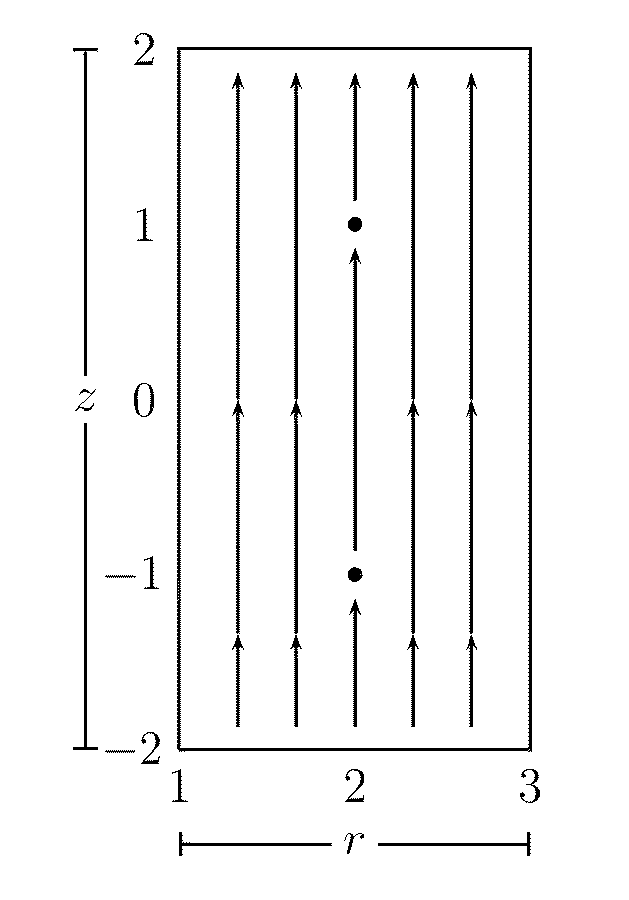
Figure 1. Vector field ${\mathcal{W}}_{v}$

The next step is to suspend the flow of the vector field ${\mathcal{W}}_{v}$ to obtain a flow on the $3$-dimensional plug. This is done as follows, where we make more precise choices of the suspension flow than given in [28], though these choices do not matter so much. Choose a $C^{\infty}$-function $f\colon{\bf R}\to[-1,1]$ which satisfies the following conditions:

1. $f(r,-z)=-f(r,z)$   [anti-symmetry in z]

2. $f(r,z)=0$ for $(r,z)$ near the boundary of ${\bf R}$

3. $f(r,z)\geq 0$ for $-2\leq z\leq 0$.

4. $f(r,z)\leq 0$ for $0\leq z\leq 2$.

5. $f(r,z)=1$ for $5/4\leq r\leq 11/4$   and   $-7/4\leq z\leq-1/4$.

6. $f(r,z)=-1$ for $5/4\leq r\leq 11/4$   and  $1/4\leq z\leq 7/4$.

Condition (W1) implies that $f(r,0)=0$ for all $1\leq r\leq 3$. The other conditions (W2), (W3), and (W4) are assumed in the works [17, 28, 34] while (W5) and (W6) were imposed in [22] in order to facilitate the description of the dynamics of the Kuperberg flows, but do not qualitatively change the resulting dynamics.

Now define the manifold with boundary

(2) $${\mathbb{W}}=[1,3]\times{\mathbb{S}}^{1}\times[-2,2]\cong{\mathbf{R}}\times{\mathbb{S}}^{1}$$

with cylindrical coordinates $x=(r,\theta,z)$. That is, ${\mathbb{W}}$ is a solid cylinder with an open core removed, obtained by rotating the rectangle ${\bf R}$, considered as embedded in ${\mathbb{R}}^{3}$, around the $z$-axis.

Extend the functions $f$ and $g$ above to ${\mathbb{W}}$ by setting $f(r,\theta,z)=f(r,z)$ and $g(r,\theta,z)=g(r,z)$, so that they are invariant under rotations around the $z$-axis. The modified Wilson vector field on ${\mathbb{W}}$ is given by

(3) $${\mathcal{W}}=g(r,\theta,z)\frac{\partial}{\partial z}+f(r,\theta,z)\frac{\partial}{\partial\theta}\ .$$

Observe that the vector field ${\mathcal{W}}$ is vertical near the boundary of ${\mathbb{W}}$ and horizontal in the periodic orbits. Also, ${\mathcal{W}}$ is tangent to the cylinders $\{r=cst\}$.

Let $\Psi_{t}$ denote the flow of ${\mathcal{W}}$ on ${\mathbb{W}}$. The flow of $\Psi_{t}$ restricted to the cylinders $\{r=cst\}$ is illustrated (in cylindrical coordinate slices) by the lines in Figures 2 and 3. The flow of $\Psi_{t}$ restricted to the cylinder $\{r=2\}$ in Figure 2(C) is a called the Reeb flow, which Schweitzer remarks in [42] was the inspiration for his introduction of this variation on the Wilson plug.

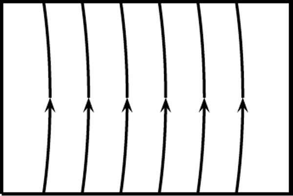
(a) $r\approx 1,3$

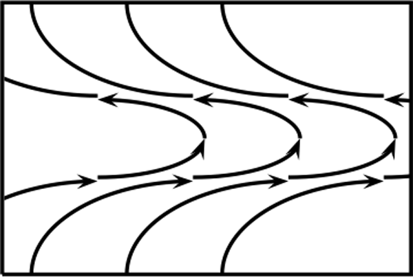
(b) $r\approx 2$

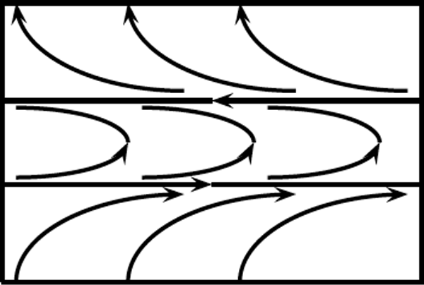
(c) $r=2$

Figure 2. ${\mathcal{W}}$-orbits on the cylinders $\{r=const.\}$

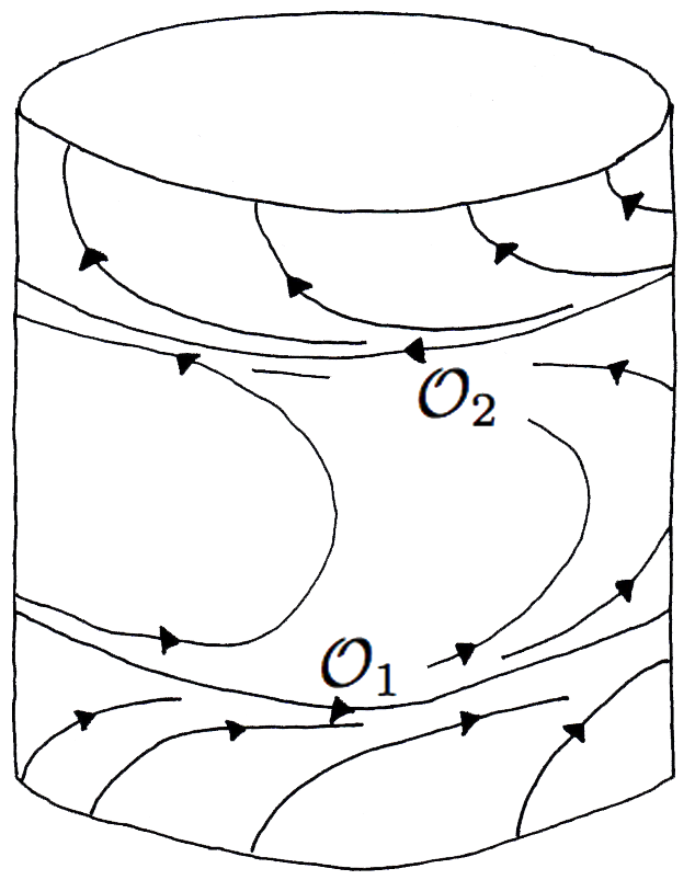
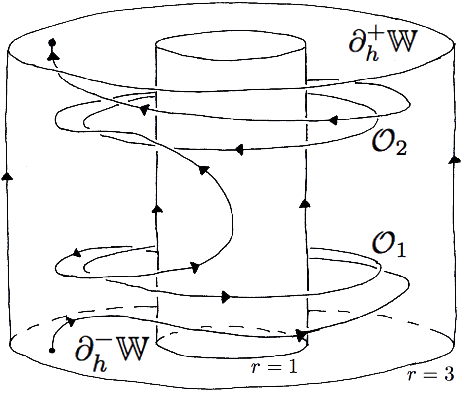
Figure 3. ${\mathcal{W}}$-orbits in the cylinder ${\mathcal{C}}=\{r=2\}$ and in ${\mathbb{W}}$

We will make reference to the following sets in ${\mathbb{W}}$:

$${\mathcal{C}}~{} \equiv ~{}\{r=2\}\quad\text{[\emph{The ~{} Full ~{} Cylinder}]}$$

$${\mathcal{R}}~{} \equiv ~{}\{(2,\theta,z)\mid-1\leq z\leq 1\}\quad\text{[\emph{The ~{} Reeb ~{} Cylinder}]}$$

$${\mathcal{A}}~{} \equiv ~{}\{z=0\}\quad\text{[\emph{The ~{} Center ~{} Annulus}]}$$

$${\mathcal{O}}_{i}~{} \equiv ~{}\{(2,\theta,(-1)^{i})\}\quad\text{[\emph{Periodic Orbits, i=1,2}]}$$

Note that ${\mathcal{O}}_{1}$ is the lower boundary circle of the Reeb cylinder ${\mathcal{R}}$, and ${\mathcal{O}}_{2}$ is the upper boundary circle.

Let us also recall some of the basic properties of the modified Wilson flow, which follow from the construction of the vector field ${\mathcal{W}}$ and the conditions (W1) to (W4) on the suspension function $f$.

Let $R_{\varphi}\colon{\mathbb{W}}\to{\mathbb{W}}$ be rotation by the angle $\varphi$. That is, $R_{\varphi}(r,\theta,z)=(r,\theta+\varphi,z)$.

PROPOSITION 2.1.

Let $\Psi_{t}$ be the flow on ${\mathbb{W}}$ defined above, then:

1. $R_{\varphi}\circ\Psi_{t}=\Psi_{t}\circ R_{\varphi}$ for all $\varphi$ and $t$.

2. The flow $\Psi_{t}$ preserves the cylinders $\{r=const.\}$ and in particular preserves the cylinders ${\mathcal{R}}$ and ${\mathcal{C}}$.

3. ${\mathcal{O}}_{i}$ for $i=1,2$ are the periodic orbits for $\Psi_{t}$.

4. For $x=(2,\theta,-2)$, the forward orbit $\Psi_{t}(x)$ for $t>0$ is trapped.

5. For $x=(2,\theta,2)$, the backward orbit $\Psi_{t}(x)$ for $t<0$ is trapped.

6. For $x=(r,\theta,z)$ with $r\neq 2$, the orbit $\Psi_{t}(x)$ terminates in the top face $\partial_{h}^{+}{\mathbb{W}}$ for some $t\geq 0$, and terminates in $\partial_{h}^{-}{\mathbb{W}}$ for some $t\leq 0$.

7. The flow $\Psi_{t}$ satisfies the entry-exit condition (P2) for plugs.

The properties of the flow $\Psi_{t}$ on ${\mathbb{W}}$ given in Proposition 2.1 are fundamental for showing that the Kuperberg flows constructed in the next section are aperiodic. On the other hand, the study of the further dynamical properties of the Kuperberg flows reveals the importance of the behavior of the flow $\Psi_{t}$ in open neighborhoods of the periodic orbits ${\mathcal{O}}_{1}$ and ${\mathcal{O}}_{2}$. This behavior depends strongly on the properties of the function $g$ in open neighborhoods of its vanishing points $(2,\pm 1)$, as will be discussed in later sections. In particular, note that if the function $g$ is modified in arbitrarily small neighborhoods of the points $(2,-1)$ and $(2,1)$, so that $g(r,z)>0$ on ${\bf R}$, then the resulting flow on ${\mathbb{W}}$ will have no periodic orbits, and no trapped orbits.

3. The Kuperberg plugs

Kuperberg’s construction in [28] of aperiodic smooth flows on plugs introduced a fundamental new idea, that of “geometric surgery” on the modified Wilson plug ${\mathbb{W}}$ constructed in the previous section, to obtain the Kuperberg Plug ${\mathbb{K}}$ as a quotient space, $\tau\colon{\mathbb{W}}\to{\mathbb{K}}$. The essence of the novel strategy behind the aperiodic property of $\Phi_{t}$ is perhaps best described by a quote from the paper by Matsumoto [34]:

We therefore must demolish the two closed orbits in the Wilson Plug beforehand. But producing a new plug will take us back to the starting line. The idea of Kuperberg is to let closed orbits demolish themselves. We set up a trap within enemy lines and watch them settle their dispute while we take no active part.

There are many choices made in the implementation of this strategy, where all such choices result in aperiodic flows. On the other hand, some of the choices appear to impact the further dynamical properties of the Kuperberg flows, as will be discussed later. We indicate in this section these alternate choices, and later formulate some of the questions which appear to be important for further study. Finally, at the end of this section, we consider flows on plugs which violate the above strategy, where the traps for the periodic orbits are purposely not aligned. This results in what we call “Derived from Kuperberg” flows, or simply DK–flows for short, which were introduced in the work [23].

The construction of a Kuperberg Plug ${\mathbb{K}}$ begins with the modified Wilson Plug ${\mathbb{W}}$ with vector field ${\mathcal{W}}$ constructed in Section 2. The first step is to re-embed the manifold ${\mathbb{W}}$ in ${\mathbb{R}}^{3}$ as a folded figure-eight, as shown in Figure 4, preserving the vertical direction.

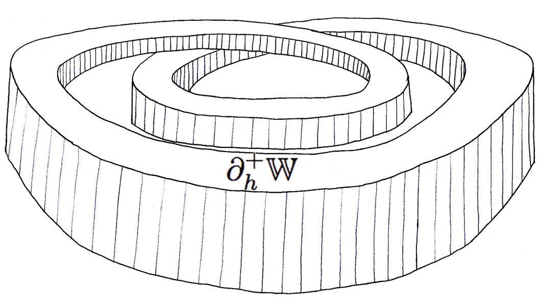
Figure 4. Embedding of Wilson Plug ${\mathbb{W}}$ as a folded figure-eight

The next step is to construct two (partial) insertions of ${\mathbb{W}}$ in itself, so that each periodic orbit of the Wilson flow is “broken open” by a trapped orbit on the self-insertion.

The construction begins with the choice in the annulus $[1,3]\times{\mathbb{S}}^{1}$ of two closed regions $L_{i}$, for $i=1,2$, which are topological disks. Each region has boundary defined by two arcs: for $i=1,2$, $\alpha^{\prime}_{i}$ is the boundary contained in the interior of $[1,3]\times{\mathbb{S}}^{1}$ and $\alpha_{i}$ in the outer boundary contained in the circle $\{r=3\}$, as depicted in Figure 5. In the work [22] the choices for these arcs are given more precisely, though for our discussion here this is not necessary.

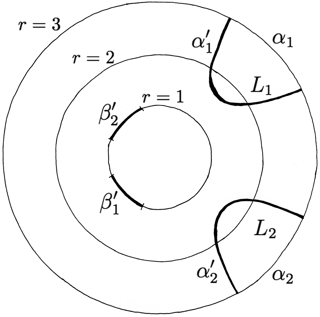
Figure 5. The disks $L_{1}$ and $L_{2}$

Consider the closed sets $D_{i}\equiv L_{i}\times[-2,2]\subset{\mathbb{W}}$, for $i=1,2$. Note that each $D_{i}$ is homeomorphic to a closed $3$-ball, that $D_{1}\cap D_{2}=\emptyset$, and each $D_{i}$ intersects the cylinder ${\mathcal{C}}=\{r=2\}$ in a rectangle. Label the top and bottom faces of these regions

(4) $$L_{1}^{\pm}=L_{1}\times\{\pm 2\}~{},~{}L_{2}^{\pm}=L_{2}\times\{\pm 2\}.$$

The next step is to define insertion maps $\sigma_{i}\colon D_{i}\to{\mathbb{W}}$, for $i=1,2$, in such a way that the periodic orbits ${\mathcal{O}}_{1}$ and ${\mathcal{O}}_{2}$ for the ${\mathcal{W}}$-flow intersect $\sigma_{i}(L_{i}^{-})$ in points corresponding to ${\mathcal{W}}$-trapped points. Consider two disjoint arcs $\beta_{i}^{\prime}$ in the inner boundary circle $\{r=1\}$ of $[1,3]\times{\mathbb{S}}^{1}$, again as depicted in Figure 5.

Now choose a smooth family of orientation preserving diffeomorphisms $\sigma_{i}\colon\alpha_{i}^{\prime}\to\beta_{i}^{\prime}$, $i=1,2$. Extend these maps to smooth embeddings $\sigma_{i}\colon D_{i}\to{\mathbb{W}}$, for $i=1,2$, as illustrated on the left-hand-side of Figure 6. We require the following conditions for $i=1,2$:

• $\sigma_{i}(\alpha_{i}^{\prime}\times z)=\beta_{i}^{\prime}\times z$ for all $z\in[-2,2]$, the interior arc $\alpha_{i}^{\prime}$ is mapped to a boundary arc $\beta_{i}^{\prime}$.

• ${\mathcal{D}}_{i}=\sigma_{i}(D_{i})$ then ${\mathcal{D}}_{1}\cap{\mathcal{D}}_{2}=\emptyset$;

• For every $x\in L_{i}$, the image ${\mathcal{I}}_{i,x}\equiv\sigma_{i}(x\times[-2,2])$ is an arc contained in a trajectory of ${\mathcal{W}}$;

• $\sigma_{1}(L_{1}\times\{-2\})\subset\{z<0\}$ and $\sigma_{2}(L_{2}\times\{2\})\subset\{z>0\}$;

• Each slice $\sigma_{i}(L_{i}\times\{z\})$ is transverse to the vector field ${\mathcal{W}}$, for all $-2\leq z\leq 2$.

• ${\mathcal{D}}_{i}$ intersects the periodic orbit ${\mathcal{O}}_{i}$ and not ${\mathcal{O}}_{j}$, for $i\neq j$.

The “horizontal faces” of the embedded regions ${\mathcal{D}}_{i}\subset{\mathbb{W}}$ are labeled by

(5) $${\mathcal{L}}_{1}^{\pm}=\sigma_{1}(L_{1}^{\pm})~{},~{}{\mathcal{L}}_{2}^{\pm}=\sigma_{2}(L_{2}^{\pm}).$$

Then the above assumptions imply that lower faces ${\mathcal{L}}_{1}^{\pm}$ intersect the first periodic orbit ${\mathcal{O}}_{1}$ and are disjoint from the second periodic orbit ${\mathcal{O}}_{2}$, while the upper faces ${\mathcal{L}}_{2}^{\pm}$ intersect ${\mathcal{O}}_{2}$ and are disjoint from ${\mathcal{O}}_{1}$.

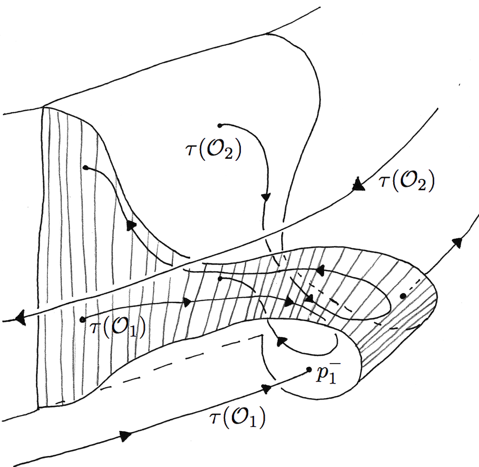
Figure 6. The image of $L_{1}\times[-2,2]$ under $\sigma_{1}$ and the radius function

The embeddings $\sigma_{i}$ are also required to satisfy two further conditions, which are the key to showing that the resulting Kuperberg flow $\Phi_{t}$ is aperiodic:

• For $i=1,2$, the disk $L_{i}$ contains a point $(2,\theta_{i})$ such that the image under $\sigma_{i}$ of the vertical segment $(2,\theta_{i})\times[-2,2]\subset D_{i}\subset{\mathbb{W}}$ is an arc $\{r=2\}\cap\{\theta_{i}^{-}\leq\theta\leq\theta_{i}^{+}\}\cap\{z=(-1)^{i}\}$ of the periodic orbit ${\mathcal{O}}_{i}$.

• Radius Inequality: For all $x^{\prime}=(r^{\prime},\theta^{\prime},z^{\prime})\in L_{i}\times[-2,2]$, let $x=(r,\theta,z)=\sigma_{i}(r^{\prime},\theta^{\prime},z^{\prime})\in{\mathcal{D}}_{i}$, then $r<r^{\prime}$ unless $x^{\prime}=(2,\theta_{i},z^{\prime})$ and then $r=r^{\prime}=2$.

The Radius Inequality (K8) is one of the most fundamental concepts of Kuperberg’s construction, and is illustrated by the graph on the right-hand-side of in Figure 6.

Condition (K4) and the fact that the flow of the vector field ${\mathcal{W}}$ on ${\mathbb{W}}$ preserves the radius coordinate on ${\mathbb{W}}$, allow restating (K8) in the more concise form for points in the faces ${\mathcal{L}}_{i}^{-}$ of the insertion regions ${\mathcal{D}}_{i}$. For $x=(r,\theta,z)=\sigma_{i}(r^{\prime},\theta^{\prime},z^{\prime})\in{\mathcal{D}}_{i}$ we have

(6) $$r(\sigma_{i}^{-1}(x))\geq r~{}{\rm for}~{}x\in{\mathcal{L}}_{i}^{-}~{},~{}{\rm with}~{}r(\sigma_{i}^{-1}(x))=r~{}{\rm if~{}and~{}only~{}if}~{}x=\sigma_{i}(2,\theta_{i},-2)~{}.$$

The illustration of the radius inequality in Figure 6 is an “idealized” case, as it implicitly assumes that the relation between the values of $r$ and $r^{\prime}$ is “quadratic” in a neighborhood of the special points $(2,\theta_{i})$, which is not required in order that (K8) be satisfied.

Finally, define ${\mathbb{K}}$ to be the quotient manifold obtained from ${\mathbb{W}}$ by identifying the sets $D_{i}$ with ${\mathcal{D}}_{i}$. That is, for each point $x\in D_{i}$ identify $x$ with $\sigma_{i}(x)\in{\mathbb{W}}$, for $i=1,2$. The restricted ${\mathcal{W}}$-flow on the inserted disk ${\mathcal{D}}_{i}=\sigma_{i}(D_{i})$ is not compatible with the image of the restricted ${\mathcal{W}}$-flow on $D_{i}$. Thus, to obtain a smooth vector field ${\mathcal{X}}$ from this construction, it is necessary to modify ${\mathcal{W}}$ on each insertion ${\mathcal{D}}_{i}$. The idea is to replace the vector field ${\mathcal{W}}$ in the interior of each region ${\mathcal{D}}_{i}$ with the image vector field and smooth the resulting piecewise continuous flow [28, 17]. Then the vector field ${\mathcal{W}}^{\prime}$ on ${\mathbb{W}}^{\prime}$ descends to a smooth vector field on ${\mathbb{K}}$ denoted by ${\mathcal{K}}$, whose flow is denoted by $\Phi_{t}$. The family of Kuperberg Plugs is the resulting space ${\mathbb{K}}\subset{\mathbb{R}}^{3}$, as illustrated in Figure 7.

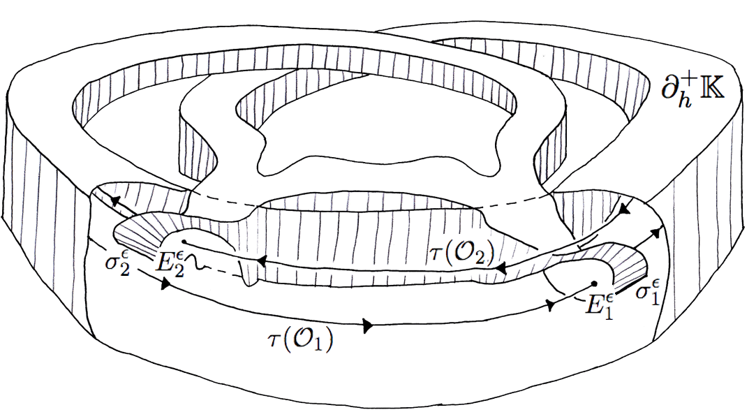
Figure 7. The Kuperberg Plug ${\mathbb{K}}_{\epsilon}$

The images in ${\mathbb{K}}$ of the cut-open periodic orbits from the Wilson flow $\Psi_{t}$ on ${\mathbb{W}}$, generate two orbits for the Kuperberg flow $\Phi_{t}$ on ${\mathbb{K}}$, which are called the special orbits for $\Phi_{t}$. These two special orbits play an absolutely central role in the study of the dynamics of the flow $\Phi_{t}$. We now state Kuperberg’s main result:

THEOREM 3.1.

[28] The flow $\Phi_{t}$ on ${\mathbb{K}}$ satisfies the conditions on a plug, and has no periodic orbits.

The papers [17, 28] remark that a Kuperberg Plug can also be constructed for which the manifold ${\mathbb{K}}$ and its flow ${\mathcal{K}}$ are real analytic. An explicit construction of such a flow is given in [29, Section 6]. There is the added difficulty that the insertion of the plug in an analytic manifold must also be analytic, which requires some subtlety. This is discussed in [29, Section 6], and also in the second author’s Ph.D. Thesis [40, Section 1.1.1].

Finally, we introduce a modification to the above construction, for which the periodic orbits of the Wilson flow are not necessarily broken open by the trapped orbits of the inserted regions. Let ${\epsilon}$ be a fixed small constant, positive or negative. Choose smooth embeddings $\sigma_{i}^{\epsilon}\colon D_{i}\to{\mathbb{W}}$, for $i=1,2$, again as illustrated on the left-hand-side of Figure 6, which satisfy the conditions (K1) to (K6). In place of the conditions (K7) and (K8), we impose the modified conditions:

• For $i=1,2$, the disk $L_{i}$ contains a point $(2,\theta_{i})$ such that the image under $\sigma_{i}^{\epsilon}$ of the vertical segment $(2,\theta_{i})\times[-2,2]\subset D_{i}\subset{\mathbb{W}}$ is an arc of a ${\mathcal{W}}$-orbit in $\{r=2+{\epsilon}\}\cap\{\theta_{i}^{-}\leq\theta\leq\theta_{i}^{+}\}$.
  

• Parametrized Radius Inequality: For all $x^{\prime}=(r^{\prime},\theta^{\prime},-2)\in L_{i}^{-}$, let $x=(r,\theta,z)=\sigma_{i}^{\epsilon}(r^{\prime},\theta^{\prime},-2)\in{\mathcal{L}}_{i}^{{\epsilon}-}$, then $r<r^{\prime}+{\epsilon}$ unless $x^{\prime}=(2,\theta_{i},-2)$ and then $r=2+{\epsilon}$.

Observe that for ${\epsilon}=0$, we recover the Radius Inequality (K8). Figure 8 represents the radius inequality for the three cases where ${\epsilon}<0$, ${\epsilon}=0$, and ${\epsilon}>0$.

(a) ${\epsilon}<0$

(b) ${\epsilon}=0$

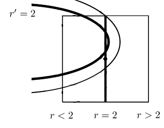
(c) ${\epsilon}>0$

Figure 8. The modified radius inequality for the cases ${\epsilon}<0$, ${\epsilon}=0$ and ${\epsilon}>0$

Again, define ${\mathbb{K}}_{\epsilon}$ to be the quotient manifold obtained from ${\mathbb{W}}$ by identifying the sets $D_{i}$ with ${\mathcal{D}}_{i}^{\epsilon}=\sigma_{i}^{\epsilon}(D_{i})$. Replace the vector field ${\mathcal{W}}$ on the interior of each region ${\mathcal{D}}_{i}^{\epsilon}$ with the image vector field and smooth the resulting piecewise continuous flow, so that we obtain a smooth vector field on ${\mathbb{K}}_{\epsilon}$ denoted by ${\mathcal{K}}_{\epsilon}$, whose flow is denoted by $\Phi_{t}^{\epsilon}$. We say that $\Phi_{t}^{\epsilon}$ is a Derived from Kuperberg flow, or a DK–flow.

The dynamics of a DK–flow is actually quite simple in the case when ${\epsilon}<0$, as shown by the following result.

THEOREM 3.2.

[23] Let ${\epsilon}<0$ and $\Phi_{t}^{\epsilon}$ be a DK–flow on ${\mathbb{K}}_{e}$. Then it satisfies the conditions on a plug, and moreover the flow in the plug ${\mathbb{K}}_{\epsilon}$ has two periodic orbits that bound an embedded invariant cylinder, and every other orbit belongs to the wandering set.

The proof of Theorem 3.2 in [23] uses the same technical tools as developed in the previous works [28, 29, 17, 34, 22] for the study of the dynamics of Kuperberg flows. In contrast, the dynamics of a DK–flow when ${\epsilon}>0$ can be quite chaotic, having positive topological entropy and have an abundance of periodic orbits, as shown by the construction of examples in [23].

4. Generic hypotheses

The construction of Kuperberg flows $\Phi_{t}$ on the plug ${\mathbb{K}}$ which satisfy Theorem 3.1 involved multiple choices, which do not change whether the resulting flows are aperiodic, but do impact other dynamical properties of these flows. In this section, we discuss in more detail these choices, and introduce the generic assumptions that were imposed in the works [22, 23]. The implications of these choices will be discussed in subsequent sections. We first discuss the choices made in constructing the modified Wilson plug, then consider the even wider range of choices involved with the construction of the insertion maps. Note that we discuss first the case for the traditional Kuperberg flows, and afterwards discuss the variations for the case of the Derived from Kuperberg flows (DK–flows).

Recall that the modified Wilson vector field on ${\mathbb{W}}$ is given in (3) by

$${\mathcal{W}}=g(r,\theta,z)\frac{\partial}{\partial z}+f(r,\theta,z)\frac{\partial}{\partial\theta}$$

where the function $g(r,\theta,z)=g(r,z)$ is the suspension of the function $g\colon{\bf R}\to[0,g_{0}]$ which is positive, except at the points $(2,\pm 1)$, and symmetric about the line $\{z=0\}$. The function $f(r,\theta,z)=f(r,z)$ is assumed to satisfy the conditions (W1) to (W6), though conditions (W5) and (W6) are imposed to simplify calculations, and do not impact the aperiodic conclusion for the Kuperberg flows.

Recall that Figure 2 illustrates the dynamics of the flow of ${\mathcal{W}}$ restricted to the cylinders $\{r=cst.\}$ in ${\mathbb{W}}$, for various values of the radius. It is clear from these pictures that the “interesting” part of the dynamics of this flow occurs on the cylinders with radius near to $2$, and near the periodic orbits ${\mathcal{O}}_{i}$ for $i=1,2$.

The points $(2,\pm 1)\in{\bf R}$ are the local minima for the function $g$, and thus its matrix of first derivatives must also vanish at these points, and the Hessian matrix of second derivatives must be positive semi-definite. The generic property for such a function is that the Hessian matrix for $g$ at these points is positive definite. In the works [22, 23], a more precise version of this was formulated:

HYPOTHESIS 4.1.

The function $g$ satisfies the following conditions:

(7) $$g(r,z)=g_{0}\quad\text{for}\quad(r-2)^{2}+(|z|-1)^{2}\geq{\epsilon}_{0}^{2}$$

where $0<{\epsilon}_{0}<1/4$ is sufficiently small. Moreover, we require that the Hessian matrices of second partial derivatives for $g$ at the vanishing points $(2,\pm 1)$ are positive definite. In addition, we require that $g(r,z)$ is monotone increasing as a function of the distance $\displaystyle\sqrt{(r-2)^{2}+(|z|-1)^{2}}$ from the points $(2,\pm 1)$.

The conclusions of Proposition 2.1 do not require Hypothesis 4.1, and so Theorem 3.1 does not require it. On the other hand, many of the results in [22, 23] do require this generic hypothesis for their proofs, as it allows making estimates on the “speed of ascent” for the orbits of the Wilson flow near the periodic orbits.

Hypothesis 4.1 implies a local quadratic estimate on the function $g$ near the points $(2,\pm 1)$ which is given as estimate (94) in [22]. We formulate a more general version of this local estimate for $g$.

HYPOTHESIS 4.2.

Let $n\geq 2$ be an even integer. Assume there exists constants $\lambda_{2}\geq\lambda_{1}>0$ and ${\epsilon}_{0}>0$ such that

(8) $$\lambda_{1}\left((r-2)^{n}+(|z|-1)^{n}\right)\leq g(r,z)\leq\lambda_{2}\left((r-2)^{n}+(|z|-1)^{n}\right)\quad{\rm for}~{}\left((r-2)^{n}+(|z|-1)^{n}\right)\leq{\epsilon}_{0}^{n+2}\ .$$

We then say that the resulting vector field ${\mathcal{W}}$ on ${\mathbb{W}}$ vanishes with order $n$.

Hypothesis 4.1 implies that Hypothesis 4.2 holds for $n=2$. This yields an estimate on the speed which the orbits of ${\mathcal{W}}$ in ${\mathbb{W}}$ for points with $z\neq\pm 1$ approach the periodic orbits ${\mathcal{O}}_{i}$ in forward or backward time, as discussed in detail in [22, Chapter 17]. When $n>2$, this speed of approach becomes slower and slower as $n$ gets larger. We can also allow for the case where $g$ has all partial derivatives vanishing at the points $(2,\pm 1)$, in which case we say that the function $g$ vanishes to infinite order at the critical points, and we say that the resulting vector field ${\mathcal{W}}$ on ${\mathbb{W}}$ infinitely flat at ${\mathcal{O}}_{i}$ for $i=1,2$. In that case, the speed of approach of orbits of ${\mathcal{W}}$ in ${\mathbb{W}}$ become arbitrarily slow towards the periodic orbits.

The choices for the embeddings $\sigma_{i}\colon D_{i}\to{\mathbb{W}}$, for $i=1,2$, as illustrated on the left-hand-side of Figure 6, are more wide-ranging, and have a fundamental influence on the dynamics of the resulting Kuperberg flows on the quotient space ${\mathbb{K}}$. We first impose a “normal form” condition on the insertions, which does not have significant impact on the dynamics, but allows a more straightforward formulation of the other properties of the insertion maps.

Let $(r,\theta,z)=\sigma_{i}(x^{\prime})\in{\mathcal{D}}_{i}$ for $i=1,2$, where $x^{\prime}=(r^{\prime},\theta^{\prime},z^{\prime})\in D_{i}$ is a point in the domain of $\sigma_{i}$. Let $\pi_{z}(r,\theta,z)=(r,\theta,-2)$ denote the projection of ${\mathbb{W}}$ along the $z$-coordinate. We assume that $\sigma_{i}$ restricted to the bottom face, $\sigma_{i}\colon L_{i}^{-}\to{\mathbb{W}}$, has image transverse to the vertical fibers of $\pi_{z}$. This normal form can be achieved by an isotopy of a given embedding along the flow lines of the vector field ${\mathcal{W}}$, so does not change the orbit structure of the resulting vector field on the plug ${\mathbb{K}}$.

The above transversality assumption implies that $\pi_{z}\circ\sigma_{i}\colon L_{i}^{-}\to{\mathbb{W}}$ is a diffeomorphism into the face $\partial_{h}^{-}{\mathbb{W}}$, with image denoted by ${\mathfrak{D}}_{i}\subset\partial_{h}^{-}{\mathbb{W}}$. Then let $\displaystyle\vartheta_{i}=(\pi_{z}\circ\sigma_{i})^{-1}\colon{\mathfrak{D}}_{i}\to L_{i}^{-}$ denote the inverse map, so we have:

(9) $$\vartheta_{i}(r,\theta,-2)=(r(\vartheta_{i}(r,\theta,-2)),\theta(\vartheta_{i}(r,\theta,-2)),-2)=(R_{i,r}(\theta),\Theta_{i,r}(\theta),-2)~{}.$$

We can then formalize in terms of the maps $\vartheta_{i}$ the assumptions on the insertion maps $\sigma_{i}$ that are intuitively implicit in Figure 6, and will be assumed for all insertion maps considered.

HYPOTHESIS 4.3 (Strong Radius Inequality).

For $i=1,2$, assume that:

1. $\sigma_{i}\colon L_{i}^{-}\to{\mathbb{W}}$ is transverse to the fibers of $\pi_{z}$;

2. $r=r(\sigma_{i}(r^{\prime},\theta^{\prime},z^{\prime}))<r^{\prime}$, except for $(2,\theta_{i},z^{\prime})$ and then $z(\sigma_{i}(2,\theta_{i},z^{\prime}))=(-1)^{i}$;

3. $\Theta_{i,r}(\theta)=\theta(\vartheta_{i}(r,\theta,-2))$ is an increasing function of $\theta$ for each fixed $r$;

4. $R_{i,r}(\theta)=r(\vartheta_{i}(r,\theta,-2))$ has non-vanishing derivative for $r=2$, except for the case of $\overline{\theta_{i}}$ defined by $\vartheta_{i}(2,\overline{\theta_{i}},-2)=(2,\theta_{i},-2)$;

5. For $r$ sufficiently close to $2$, we require that the $\theta$ derivative of $R_{i,r}(\theta)$ vanish at a unique point denoted by $\overline{\theta}(i,r)$.

Consequently, each surface ${\mathcal{L}}_{i}^{-}$ is transverse to the coordinate vector fields $\partial/\partial\theta$ and $\partial/\partial z$ on ${\mathbb{W}}$.

The illustration of the image of the curves $r^{\prime}=2$ and $r^{\prime}=3$ on the right-hand-side of Figure 6 suggests that these curves have “parabolic shape”. We formulate this notion more precisely using the function $\vartheta_{i}(r,\theta,-2)$ defined by (9), and introduce the more general hypotheses they may satisfy. Recall that ${\epsilon}_{0}>0$ was introduced in Hypothesis 4.1.

HYPOTHESIS 4.4.

Let $n\geq 2$ be an even integer. For $i=1,2$, $2\leq r_{0}\leq 2+{\epsilon}_{0}$ and $\theta_{i}-{\epsilon}_{0}\leq\theta\leq\theta_{i}+{\epsilon}_{0}$, assume that

(10) $$\frac{d}{d\theta}\Theta_{i,r_{0}}(\theta)>0\quad,\quad\frac{d^{n}}{d\theta^{n}}R_{i,r_{0}}(\theta)>0\quad,\quad\frac{d}{d\theta}R_{i,r_{0}}(\overline{\theta_{i}})=0\quad,\quad\frac{d^{\ell}}{d\theta^{\ell}}R_{i,r_{0}}(\overline{\theta_{i}})=0~{}{\rm for}~{}1\leq\ell<n\ .$$

where $\overline{\theta_{i}}$ satisfies $\vartheta_{i}(2,\overline{\theta_{i}},-2)=(2,\theta_{i},-2)$. Thus for $2\leq r_{0}\leq 2+{\epsilon}_{0}$, the graph of $R_{i,r_{0}}(\theta)$ is convex upwards with vertex at $\theta=\overline{\theta_{i}}$.

In the case where $n=2$, Hypothesis 4.4 implies that all of the level curves $r^{\prime}=c$, for $2\leq c\leq 2+{\epsilon}_{0}$, have parabolic shape, as the illustration in Figure 6 suggests. On the other hand, for $n>2$ the level curves $r^{\prime}=c$ have higher order contact with the vertical lines of constant radius in Figure 6, and in this case, many of the dynamical properties of the resulting flow $\Phi_{t}$ on ${\mathbb{K}}$ are not well-understood.

We can now define what is called a generic Kuperberg flow in the work [22].

DEFINITION 4.5.

A Kuperberg flow $\Phi_{t}$ is generic if the Wilson flow ${\mathcal{W}}$ used in the construction of the vector field ${\mathcal{K}}$ satisfies Hypothesis 4.1, and the insertion maps $\sigma_{i}$ for $i=1,2$ used in the construction of ${\mathbb{K}}$ satisfies Hypotheses 4.3, and Hypotheses 4.4 for $n=2$. That is, the singularities for the vanishing of the vertical component $g\cdot\partial/\partial z$ of the vector field ${\mathcal{W}}$ are of quadratic type, and the insertion maps used to construct ${\mathbb{K}}$ yield quadratic radius functions near the special points.

Recall that the insertion maps for a Derived from Kuperberg flow as introduced in Section 3 are denoted by $\sigma_{i}^{\epsilon}\colon D_{i}\to{\mathbb{W}}$, for $i=1,2$. It is assumed that these maps satisfy the modified conditions (K7${\epsilon}$) and (K8${\epsilon}$). The illustrations of the radius inequality in Figure 8 again suggest that the images of the curves $r^{\prime}=c$ are of “quadratic type”, though the vertex of the image curves need no longer be at a special point. We again assume the insertion maps $\sigma_{i}^{\epsilon}\colon L_{i}^{-}\to{\mathbb{W}}$ are transverse to the fibers of the projection map $\pi_{z}\colon{\mathbb{W}}\to\partial_{h}^{-}{\mathbb{W}}$ along the $z^{\prime}$-coordinate. Then we can define the inverse map $\vartheta_{i}^{\epsilon}=(\pi_{z}\circ\sigma_{i}^{\epsilon})^{-1}\colon{\mathfrak{D}}_{i}\to L_{i}^{-}$ and express the inverse map $x^{\prime}=\vartheta_{i}^{\epsilon}(x)$ in polar coordinates as:

(11) $$x^{\prime}=(r^{\prime},\theta^{\prime},-2)=\vartheta_{i}^{\epsilon}(r,\theta,-2)=(r(\vartheta_{i}^{\epsilon}(r,\theta,-2)),\theta(\vartheta_{i}^{\epsilon}(r,\theta,-2)),-2)=(R_{i,r}^{\epsilon}(\theta),\Theta_{i,r}^{\epsilon}(\theta),-2)~{}.$$

Then the level curves $r^{\prime}=c$ pictured in Figure 8 are given by the maps $\theta^{\prime}\mapsto\pi_{z}(\sigma_{i}^{\epsilon}(c,\theta^{\prime},-2))\in\partial_{h}^{-}{\mathbb{W}}$.

We note a straightforward consequence of the Parametrized Radius Inequality (K8${\epsilon}$). Recall that $\theta_{i}$ is the radian coordinate specified in (K8${\epsilon}$) such that for $x^{\prime}=(2,\theta_{i},-2)\in L_{i}^{-}$ we have $r(\sigma_{i}^{\epsilon}(2,\theta_{i},-2))=2+{\epsilon}$.

LEMMA 4.6.

[23, Lemma 6.1] For ${\epsilon}>0$ there exists $2+{\epsilon}<r_{\epsilon}<3$ such that $r(\sigma_{i}^{\epsilon}(r_{\epsilon},\theta_{i},-2))=r_{\epsilon}$.

We then add an additional assumption on the insertion maps $\sigma_{i}^{\epsilon}$ for $i=1,2$ which specifies the qualitative behavior of the radius function for $r\geq r_{\epsilon}$.

HYPOTHESIS 4.7.

If $r_{\epsilon}$ is the smallest $2+{\epsilon}<r_{\epsilon}<3$ such that $r(\sigma_{i}^{\epsilon}(r_{\epsilon},\theta_{i},-2))=r_{\epsilon}$. Assume that $r(\sigma_{i}^{\epsilon}(r,\theta_{i},-2))<r$ for $r>r_{\epsilon}$.

The conclusion of Hypothesis 4.7 is implied by the Radius Inequality for the case ${\epsilon}=0$, but does not follow from the condition (K8${\epsilon}$) when ${\epsilon}>0$. It is imposed to eliminate some of the possible pathologies in the behavior of the orbits of the DK–flows.

We can now formulate the analog for DK–flows of the Hypothesis 4.3, which imposes uniform conditions on the derivatives of the maps $\vartheta_{i}^{\epsilon}$. Recall that $0<{\epsilon}_{0}<1/4$ was specified in Hypothesis 4.1, and we assume that $0<{\epsilon}<{\epsilon}_{0}$.

HYPOTHESIS 4.8 (Strong Radius Inequality).

For $i=1,2$, assume that:

1. $\sigma_{i}^{\epsilon}\colon L_{i}^{-}\to{\mathbb{W}}$ is transverse to the fibers of $\pi_{z}$;

2. $r=r(\sigma_{i}^{\epsilon}(r^{\prime},\theta^{\prime},z))<r+{\epsilon}$, except for $x^{\prime}=(2,\theta_{i},z)$ and then $r=2+{\epsilon}$;

3. $\Theta_{i,r}^{\epsilon}(\theta)$ is an increasing function of $\theta$ for each fixed $r$;

4. For $2-{\epsilon}_{0}\leq r\leq 2+{\epsilon}_{0}$ and $i=1,2$, assume that $R_{i,r}^{\epsilon}(\theta)$ has non-vanishing derivative, except when $\theta=\overline{\theta_{i}}$ as defined by $\vartheta_{i}^{\epsilon}(2+{\epsilon},\overline{\theta}_{i},-2)=(2,\theta_{i},-2)$;

5. For $r$ sufficiently close to $2+{\epsilon}$, we require that the $\theta$ derivative of $R_{i,r}^{\epsilon}(\theta)$ vanishes at a unique point denoted by $\overline{\theta}(i,r)$.

Note that Hypotheses 4.7 and 4.8 combined imply that $r_{\epsilon}$ is the unique value of $2+{\epsilon}<r_{\epsilon}<3$ for which $r(\sigma_{i}^{\epsilon}(r_{\epsilon},\theta_{i},-2))=r_{\epsilon}$. We can then formulate the analog of Hypothesis 4.4.

HYPOTHESIS 4.9.

Let $n\geq 2$ be an even integer. For $2-{\epsilon}_{0}\leq r_{0}\leq 2+{\epsilon}_{0}$ and $\theta_{i}-{\epsilon}_{0}\leq\theta\leq\theta_{i}+{\epsilon}_{0}$, assume that

(12) $$\frac{d}{d\theta}\Theta_{i,r_{0}}^{\epsilon}(\theta)>0\quad,\quad\frac{d^{n}}{d\theta^{n}}R_{i,r_{0}}^{\epsilon}(\theta)>0\quad,\quad\frac{d}{d\theta}R_{i,r_{0}}^{\epsilon}(\overline{\theta_{i}})=0\quad,\quad\frac{d^{\ell}}{d\theta^{\ell}}R_{i,r_{0}}^{\epsilon}(\overline{\theta_{i}})=0~{}{\rm for}~{}1\leq\ell<n\ .$$

where $\overline{\theta_{i}}$ satisfies $\vartheta_{i}^{\epsilon}(2,\overline{\theta_{i}},-2)=(2,\theta_{i},-2)$. Thus for $2-{\epsilon}_{0}\leq r_{0}\leq 2+{\epsilon}_{0}$, the graph of $R_{i,r_{0}}^{\epsilon}(\theta)$ is convex upwards with vertex at $\theta=\overline{\theta_{i}}$.

Finally, we have the definition of the generic DK–flows studied in [23].

DEFINITION 4.10.

A DK–flow $\Phi_{t}^{\epsilon}$ is generic if the Wilson flow ${\mathcal{W}}$ used in the construction of the vector field ${\mathcal{K}}$ satisfies Hypothesis 4.1, and the insertion maps $\sigma_{i}^{\epsilon}$ for $i=1,2$ used in the construction of ${\mathbb{K}}$ satisfies Hypotheses 4.8, and Hypotheses 4.9 for $n=2$.

5. Wandering and minimal sets

We next discuss some of the basic topological dynamics properties the Kuperberg flows in plugs. Our main interest is in the asymptotic behavior of their orbits, especially the non-wandering and wandering sets for the flow. There is an additional subtlety in these considerations, in that many orbits for the flow in a plug may escape from the plug, while other orbits are trapped in either the forward or backward directions, or possibly both. We also recall the results about the uniqueness of the minimal set. First we recall some of the basic concepts for the flow in a plug.

Recall that ${\mathcal{D}}_{i}=\sigma_{i}(D_{i})$ for $i=1,2$ are solid $3$-disks embedded in ${\mathbb{W}}$. Introduce the sets:

(13) $${\mathbb{W}}^{\prime}~{}\equiv~{}{\mathbb{W}}-\left\{{\mathcal{D}}_{1}\cup{\mathcal{D}}_{2}\right\}\quad,\quad\widehat{{\mathbb{W}}}~{}\equiv~{}\overline{{\mathbb{W}}-\left\{{\mathcal{D}}_{1}\cup{\mathcal{D}}_{2}\right\}}~{}.$$

The compact space $\widehat{{\mathbb{W}}}\subset{\mathbb{W}}$ is the result of “drilling out” the interiors of ${\mathcal{D}}_{1}$ and ${\mathcal{D}}_{2}$.

Let $\tau\colon{\mathbb{W}}\to{\mathbb{K}}$ denote the quotient map. Note that the restriction $\tau^{\prime}\colon{\mathbb{W}}^{\prime}\to{\mathbb{K}}$ is injective and onto, while for $i=1,2$, the map $\tau$ identifies a point $x\in D_{i}$ with its image $\sigma_{i}(x)\in{\mathcal{D}}_{i}$. Let $(\tau^{\prime})^{-1}\colon{\mathbb{K}}\to{\mathbb{W}}^{\prime}$ denote the inverse map, which followed by the inclusion ${\mathbb{W}}^{\prime}\subset{\mathbb{W}}$, yields the (discontinuous) map $\tau^{-1}\colon{\mathbb{K}}\to{\mathbb{W}}$, where $i=1,2$, we have:

(14) $$\tau^{-1}(\tau(x))=x~{}{\rm for}~{}x\in D_{i}~{},~{}{\rm and}~{}\sigma_{i}(\tau^{-1}(\tau(x)))=x~{}{\rm for}~{}x\in{\mathcal{D}}_{i}~{}.$$

Consider the embedded disks ${\mathcal{L}}_{i}^{\pm}\subset{\mathbb{W}}$ defined by (5), which appear as the faces of the insertions in ${\mathbb{W}}$. Their images in the quotient manifold ${\mathbb{K}}$ are denoted by:

(15) $$E_{1}=\tau({\mathcal{L}}_{1}^{-})~{},~{}S_{1}=\tau({\mathcal{L}}_{1}^{+})~{},~{}E_{2}=\tau({\mathcal{L}}_{2}^{-})~{},~{}S_{2}=\tau({\mathcal{L}}_{2}^{+})~{}.$$

Note that $\tau^{-1}(E_{i})=L_{i}^{-}$, while $\tau^{-1}(S_{i})=L_{i}^{+}$.

The transition points of an orbit of $\Phi_{t}$ are those points where the orbit intersects one of the sets $E_{i}$ or $S_{i}$ for $i=1,2$, or is contained in a boundary component $\partial_{h}^{-}{\mathbb{K}}$ or $\partial_{h}^{+}{\mathbb{K}}$. The transition points are classified as either primary or secondary, where $x\in{\mathbb{K}}$ is:

• a primary entry point if $x\in\partial_{h}^{-}{\mathbb{K}}$;

• a primary exit point if $x\in\partial_{h}^{+}{\mathbb{K}}$;

• a secondary entry point if $x\in E_{1}\cup E_{2}$;

• a secondary exit point $x\in S_{1}\cup S_{2}$.

If a $\Phi_{t}$-orbit of a point $x\in{\mathbb{K}}$ contains no transition points, then the restriction $\tau^{-1}(\Phi_{t}(x))$ is a continuous function of $t$, and in fact is contained in the $\Psi_{t}$-orbit of $x^{\prime}=\tau^{-1}(x)\in{\mathbb{W}}$.

Recall that $r\colon{\mathbb{W}}\to[1,3]$ is the radius coordinate on ${\mathbb{W}}$. Define the (discontinuous) radius coordinate $r\colon{\mathbb{K}}\to[1,3]$, where for $x\in{\mathbb{K}}$ set $r(x)=r(\tau^{-1}(x))$. Then for $x\in{\mathbb{K}}$ set $\rho_{x}(t)\equiv r(\Phi_{t}(x))$, which is the radius coordinate function along the ${\mathcal{K}}$-orbit of $x$. Note that if $\Phi_{t_{0}}(x)$ is not an entry/exit point, then the function $\rho_{x}(t)$ is locally constant at $t_{0}$. On the other hand, if $t_{0}$ is a point of discontinuity for $\Phi_{t}(x)$, then $x_{0}=\Phi_{t_{0}}(x)$ must be a secondary entry or exit point.

These properties of the radius function along orbits of the flow $\Phi_{t}$ gives a strategy for the study of the dynamics of the flow, and in fact provides the key technique in [28] used to prove that the flow is aperiodic. A key idea is to index the points along the orbit of a point $x\in{\mathbb{K}}$ by the intersections with the sets $E_{1}\cup E_{2}$, for which the index increases by $+1$, or by their intersection with the sets $S_{1}\cup S_{2}$, for which the index decreases by $-1$. This yields the integer-valued level function $n_{x}(t)$ which has $n_{x}(0)=0$.

Recall that ${\mathcal{O}}_{i}$ for $i=1,2$ denotes the periodic orbits for the Wilson flow on ${\mathbb{W}}$, so that each intersection ${\mathcal{O}}_{i}\cap{\mathbb{W}}^{\prime}$ consists of an open connected arc with endpoints ${\mathcal{L}}_{i}^{\pm}\cap{\mathcal{O}}_{i}$. The special entry/exit points for the flow $\Phi_{t}$ are the images, for $i=1,2$,

(16) $$p_{i}^{-}=\tau({\mathcal{O}}_{i}\cap{\mathcal{L}}_{i}^{-})\in E_{i}~{},~{}p_{i}^{+}=\tau({\mathcal{O}}_{i}\cap{\mathcal{L}}_{i}^{+})\in S_{i}~{}.$$

Note that by definitions and the Radius Inequality, we have $r(p_{i}^{\pm})=2$ for $i=1,2$.

We now recall the results for the minimal set of Kuperberg flows based on the combined results from the works [17, 28, 29, 34]. It was observed by Kuperberg in [28] that for $x\in{\mathbb{K}}$ with $r(x)=2$, then either its forward orbit $\{\Phi_{t}(x)\mid t\geq 0\}$ contains a special point in its closure, or this is true for the backward orbit $\{\Phi_{t}(x)\mid t\leq 0\}$, or both conditions hold. Also, for $x\in{\mathbb{K}}$ if the radius function $\rho_{x}(t)\geq c$ for some $c>2$, then the orbit of $x$ escapes in finite time in both forward and backward directions. It follows from this that for $x\in{\mathbb{K}}$ with $r(x)>2$ and whose orbit is infinite in either forward or backward directions, then its orbit closure must contain at least one of the special orbits.

It was observed in Matsumoto [34] that there is an open set of primary entry points with radius less than $2$ whose forward orbits are non-recurrent and yet accumulate on the special orbits. Ghys showed in [17, Théorème, page 301] that if $x\in{\mathbb{K}}$ does not escape from ${\mathbb{K}}$ in a finite time, either forward or backward, then the orbit of the point accumulates on (at least one) of the special orbits. These results combined imply that a Kuperberg flow has a unique minimal set contained in the interior of ${\mathbb{K}}$.

We state these results more succinctly as follows. Define the following orbit closures in ${\mathbb{K}}$:

(17) $$\Sigma_{1}~{}\equiv~{}\overline{\{\Phi_{t}(p_{1}^{-})\mid-\infty<t<\infty\}}\quad,\quad\Sigma_{2}~{}\equiv~{}\overline{\{\Phi_{t}(p_{2}^{-})\mid-\infty<t<\infty\}}~{}.$$

THEOREM 5.1.

[22, Theorem 8.2] For the closed sets $\Sigma_{i}$ for $i=1,2$ we have:

1. $\Sigma_{i}$ is $\Phi_{t}$-invariant;

2. $r(x)\geq 2$ for all $x\in\Sigma_{i}$;

3. $\Sigma_{1}=\Sigma_{2}$ and we set $\Sigma=\Sigma_{1}=\Sigma_{2}$;

4. Let ${\mathcal{Z}}\subset{\mathbb{K}}$ be a closed invariant set for $\Phi_{t}$ contained in the interior of ${\mathbb{K}}$, then $\Sigma\subset{\mathcal{Z}}$;

5. $\Sigma$ is the unique minimal set for $\Phi_{t}$.

Note that for the Wilson plug [48], the flow has two minimal sets, consisting of closed orbits, while the Schweitzer plug [42] has also two minimal sets homeomorphic to a Denjoy minimal set in the $2$-torus. On the other hand, the topological type of the unique minimal set $\Sigma$ for a Kuperberg flow is extraordinarily complicated, and seems to require additional generic hypotheses on the construction of the flow to gain a deeper understanding of its topological properties.

The orbits of the Kuperberg flow are divided into those which are finite, forward or backward trapped, or trapped in both directions and so infinite. A point $x\in{\mathbb{K}}$ is forward wandering if there exists an open set $x\in U\subset{\mathbb{K}}$ and $T_{U}>0$ so that for all $t\geq T_{U}$ we have $\Phi_{t}(U)\cap U=\emptyset$. Similarly, $x$ is backward wandering if there exists an open set $x\in U\subset{\mathbb{K}}$ and $T_{U}<0$ so that for all $t\leq T_{U}$ we have $\Phi_{t}(U)\cap U=\emptyset$. A point $x$ with infinite orbit is wandering if it is forward and backward wandering. Define the following subsets of ${\mathbb{K}}$:

$${\mathfrak{W}}^{0} \equiv \{x\in{\mathbb{K}}\mid x~{}{\rm orbit~{}is~{}finite}\}$$

$${\mathfrak{W}}^{+} \equiv \{x\in{\mathbb{K}}\mid x~{}{\rm orbit~{}is~{}forward~{}wandering}\}$$

$${\mathfrak{W}}^{-} \equiv \{x\in{\mathbb{K}}\mid x~{}{\rm orbit~{}is~{}backward~{}wandering}\}$$

$${\mathfrak{W}}^{\infty} \equiv \{x\in{\mathbb{K}}\mid x~{}\mbox{ is forward and backward wandering}\}$$

Note that $x\in{\mathfrak{W}}^{0}$ if and only if the orbit of $x$ escapes through $\partial_{h}^{+}{\mathbb{K}}$ in forward time, and escapes though $\partial_{h}^{-}{\mathbb{K}}$ in backward time. Define

(18) $${\mathfrak{W}}~{}=~{}{\mathfrak{W}}^{0}\cup{\mathfrak{W}}^{+}\cup{\mathfrak{W}}^{-}\cup{\mathfrak{W}}^{\infty}\quad;\quad\Omega={\mathbb{K}}-{\mathfrak{W}}.$$

The set $\Omega$ is called the non-wandering set for $\Phi_{t}$, is closed and $\Phi_{t}$-invariant. A point $x$ with forward trapped orbit is characterized by the property: $x\in\Omega$ if for all ${\epsilon}>0$ and $T>0$, there exists $y$ and $t>T$ such that $d_{{\mathbb{K}}}(x,y)<{\epsilon}$ and $d_{{\mathbb{K}}}(x,\Phi_{t}(y))<{\epsilon}$, where $d_{{\mathbb{K}}}$ is a distance function on ${\mathbb{K}}$. There are obvious corresponding statements for points which are backward trapped or infinite. Here are some of the properties of the wandering and non-wandering sets for Kuperberg flows. The proofs can be found in [22, Chapter 8].

LEMMA 5.2.

If $x\in{\mathbb{K}}$ is a primary entry or exit point, then $x\in{\mathfrak{W}}^{+}$ or ${\mathfrak{W}}^{-}$.

LEMMA 5.3.

For each $x\in\Omega$, the $\Phi_{t}$-orbit of $x$ is infinite.

PROPOSITION 5.4.

$\Sigma\subset\Omega\subset\{x\in{\mathbb{K}}\mid r(x)\geq 2\}$.

Finally, let us recall a result of Matsumoto:

THEOREM 5.5.

[34, Theorem 7.1(b)] The sets ${\mathfrak{W}}^{\pm}$ contain interior points.

This implies the following important consequence:

COROLLARY 5.6.

The flow $\Phi_{t}$ cannot preserve any smooth invariant measure on ${\mathbb{K}}$ which assigns positive mass to any neighborhood of a special point.

At this point it is worth mentioning one of the big open problems regarding the existence of periodic orbits for flows on 3-manifolds. For volume preserving vectors fields that are at least $C^{2}$, it is unknown whether they must have periodic orbits. G. Kuperberg proved two important results: first every 3-manifold admits a volume-preserving $C^{\infty}$ vector field that has a finite number of periodic orbits, and second that there are volume-preserving $C^{1}$-flows without periodic orbits [30]. These results are based on the use of plugs.

6. Zippered laminations

We next introduce the $\Phi_{t}$-invariant embedded surface ${\mathfrak{M}}_{0}$ and its closure ${\mathfrak{M}}$, and discuss the relation between the minimal set $\Sigma$ and the space ${\mathfrak{M}}$. The existence of this compact connected subset ${\mathfrak{M}}$ which is invariant for the Kuperberg flow $\Phi_{t}$ is a remarkable consequence of the construction, and is the key to a deeper understanding of the properties of the minimal set $\Sigma$ of $\Phi_{t}$. We then give an overview of the structure theory for ${\mathfrak{M}}_{0}$ which plays a fundamental role in analyzing the dynamical properties of Kuperberg flows.

Recall that the Reeb cylinder ${\mathcal{R}}\subset{\mathbb{W}}$ is bounded by the two periodic orbits ${\mathcal{O}}_{1}$ and ${\mathcal{O}}_{2}$ for the Wilson flow $\Psi_{t}$ on ${\mathbb{W}}$. The cylinder ${\mathcal{R}}$ is itself invariant under this flow, and for a point $x\in{\mathbb{W}}$ with $r(x)$ close to $2$, the $\Psi_{t}$-orbit of $x$ has increasing long orbit segments which shadow the periodic orbits. Since the special orbits in ${\mathbb{K}}$ contain the intersection $\tau({\mathcal{O}}_{i}\cap{\mathbb{W}}^{\prime})$ for $i=1,2$, they are contained in the ${\mathcal{K}}$-orbits of the set obtained by flowing the Reeb cylinder $\tau({\mathcal{R}}\cap{\mathbb{W}}^{\prime})$.

Introduce the notched Reeb cylinder, ${\mathcal{R}}^{\prime}={\mathcal{R}}\cap{\mathbb{W}}^{\prime}$, which has two closed “notches” removed from ${\mathcal{R}}$ where it intersects the closed insertions ${\mathcal{D}}_{i}\subset{\mathbb{W}}$ for $i=1,2$. Figure 9 illustrates the cylinder ${\mathcal{R}}^{\prime}$ inside ${\mathbb{W}}$. The boundary segments $\gamma^{\prime}$ and $\lambda^{\prime}$ labeled in Figure 9 satisfy $\gamma^{\prime}\subset{\mathcal{L}}_{1}^{-}$ and $\lambda^{\prime}\subset{\mathcal{L}}_{2}^{-}$, while the boundary segments $\overline{\gamma}^{\prime}$ and $\overline{\lambda}^{\prime}$ labeled in Figure 9 satisfy $\overline{\gamma}^{\prime}\subset{\mathcal{L}}_{1}^{+}$ and $\overline{\lambda}^{\prime}\subset{\mathcal{L}}_{2}^{+}$. A basic observation is that these curves are each transverse to the restriction of the Wilson flow to the cylinder ${\mathcal{R}}$.

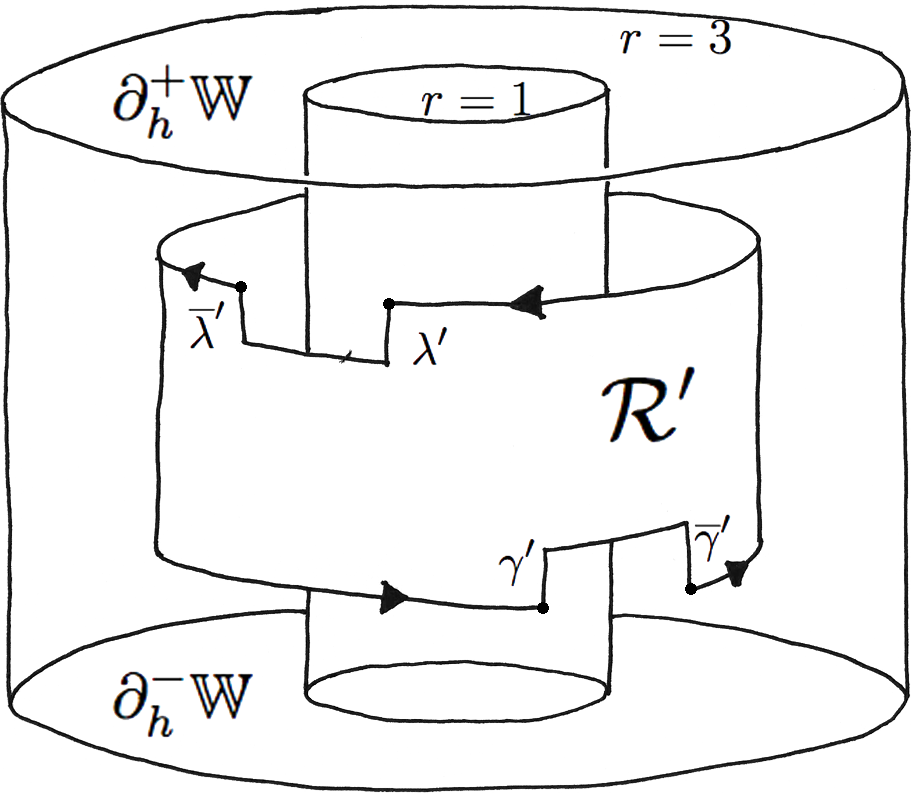
Figure 9. The notched cylinder ${\mathcal{R}}^{\prime}$ embedded in ${\mathbb{W}}$

The map $\tau\colon{\mathcal{R}}^{\prime}\to{\mathbb{K}}$ is an embedding, so the $\Phi_{t}$-flow of $\tau({\mathcal{R}}^{\prime})\subset{\mathbb{K}}$ is an embedded surface,

(19) $${\mathfrak{M}}_{0}~{}\equiv~{}\{\Phi_{t}(\tau({\mathcal{R}}^{\prime}))\mid-\infty<t<\infty\}~{}.$$

The “boundary” of ${\mathfrak{M}}_{0}$ consists of the two special orbits in ${\mathbb{K}}$ obtained by the $\Phi_{t}$-flows of the arcs $\tau({\mathcal{O}}_{i}\cap{\mathbb{W}}^{\prime})$ for $i=1,2$, so that ${\mathfrak{M}}_{0}$ is an “infinite bordism” between the two special orbits of the flow $\Phi_{t}$. Thus, the closure ${\mathfrak{M}}=\overline{{\mathfrak{M}}_{0}}$ is a flow invariant, compact connected subset of ${\mathbb{K}}$, which contains the closure of the special orbits, hence by Theorem 5.1, the minimal set $\Sigma\subset{\mathfrak{M}}$. A fundamental problem is then to give a description of the topology and geometry of the space ${\mathfrak{M}}$. The question of when $\Sigma={\mathfrak{M}}$ is treated in Section 7, while in this section we concentrate on the properties of ${\mathfrak{M}}$.

The key to understanding the structure of the space ${\mathfrak{M}}$ is to analyze the structure of ${\mathfrak{M}}_{0}$ and its embedding in ${\mathbb{K}}$. This analysis is based on a simple observation, that the images $\tau(\gamma^{\prime}),\tau(\lambda^{\prime})\subset{\mathfrak{M}}$ are curves transverse to the flow $\Phi_{t}$ and contained in the region $\{x\in{\mathfrak{M}}\mid r(x)\geq 2\}$. Moreover, for a point $x\in\tau(\gamma^{\prime})$ with $r(x)>2$, there is a finite $t_{x}>0$ such that $\Phi_{t_{x}}(x)\in\tau(\overline{\gamma}^{\prime})$. That is, the flow across the notch in $\tau({\mathcal{R}}^{\prime})$ with boundary curve $\tau(\gamma^{\prime})$ closes up by returning to the facing boundary curve $\tau(\overline{\gamma}^{\prime})$, unless $r(x)=2$ and then $x$ is the special point $p_{1}^{-}$. A similar remark holds for the notch in ${\mathcal{R}}^{\prime}$ with boundary curves $\lambda^{\prime},\overline{\lambda}^{\prime}$. It follows from the proof of the above remarks that we can use a recursive approach to analyze the submanifold ${\mathfrak{M}}_{0}$, decomposing the space into the flows in ${\mathbb{K}}$ of the curves of successive intersections with the entry/exit surfaces $E_{i}$ and $S_{i}$.

PROPOSITION 6.1.

[22, Proposition 10.1] There is a well-defined level function

(20) $$n_{0}\colon{\mathfrak{M}}_{0}\to{\mathbb{N}}=\{0,1,2,\ldots\}\ ,$$

where the preimage $n_{0}^{-1}(0)=\tau({\mathcal{R}}^{\prime})$, the preimage $n_{0}^{-1}(1)$ in the union of two infinite propellers which are asymptotic to $\tau({\mathcal{R}}^{\prime})$, and for $\ell>1$ the preimage $n_{0}^{-1}(\ell)$ is a countable union of finite propellers.

The precise description of propellers, both finite and infinite, is given in [22, Chapters 11, 12], and the decomposition is made precise there. We give a general sketch of the idea.

A propeller is an embedded surface in ${\mathbb{W}}$ that results from the Wilson flow $\Psi_{t}$ of a curve $\gamma\subset\partial_{h}^{-}{\mathbb{W}}$ in the bottom face of ${\mathbb{W}}$. Such a surface has the form of a “tongue” wrapping around the core cylinder ${\mathcal{C}}$. Figure 10 illustrates a “typical” finite propeller $P_{{\gamma}}$ as a compact “flattened” propeller on the right, and its embedding in ${\mathbb{W}}$ on the left. Observe that for any $x\in{\gamma}$ the radius of $x$ is strictly bigger than 2. An infinite propeller is not closed, and its boundary curve is the orbit of an entry point with radius $2$, hence limits on the Reeb cylinder ${\mathcal{R}}$. The embedding of an infinite propeller is highly dependent on the shape of the curve $\gamma$ near the cylinder ${\mathcal{C}}$, and on the dynamics of the Wilson flow near its periodic orbits.

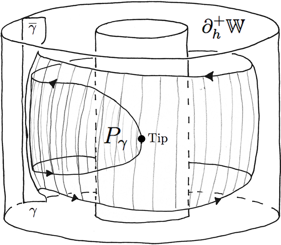
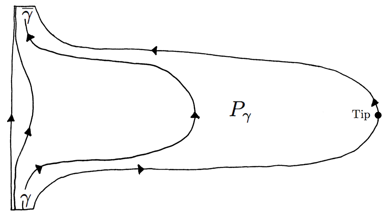
Figure 10. Embedded and flattened finite propeller

Figure 11 gives a model for ${\mathfrak{M}}_{0}$, though the distances along propellers are not to scale, and there is a hidden simplification in that there may be “bubbles” in the surfaces which are suppressed in the illustration. A bubble is a branching surface attached to the interior regions of a propeller, and are analyzed in Chapters 15 and 18 of [22]. Also, all the propellers represented in Figure 11 have roughly the same width when embedded in ${\mathbb{K}}$, which is the width of the Reeb cylinder.

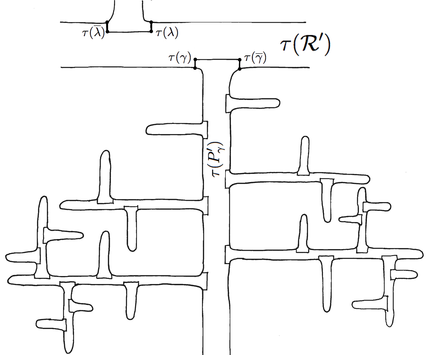
Figure 11. Flattened part of ${\mathfrak{M}}_{0}$

We make some further comments on the properties of ${\mathfrak{M}}_{0}$ as illustrated in Figure 11. The upper horizontal band the figure represents the notched Reeb cylinder. The flow of the special point $p_{1}^{-}$ is the curve along the bottom edge of the image $\tau({\mathcal{R}}^{\prime})$. When the flow crosses the curve $\tau(\gamma)=\tau({\mathcal{R}}^{\prime})\cap E_{1}$, it turns to the right and enters the infinite propeller at level $1$, and follows the left edge of this vertical strip downward, along the Wilson flow of a point with $r=2$ until it intersects the secondary entry surface $E_{1}$ again. It then turns to the right in the flow direction, and enters a finite propeller at level $2$. In the case pictured, it then flows upward until it crosses the annulus ${\mathcal{A}}=\{z=0\}\subset{\mathbb{W}}$, which corresponds to the tip of the propeller. It then reverses direction and flows until it crosses the secondary exit surface $S_{1}$, and resumes flowing downward along the infinite level $1$ propeller. However, as this is following a Wilson orbit, the $z$-values of this part of the orbit are increasing towards $-1$.

This procedure continues repeatedly, though as the curve moves further down the level $1$ propeller, the $z$-values get closer to $-1$, and hence the flow in the side level 2 propellers intersects the secondary entry region $E_{1}$ increasingly often, before flowing through the tip of the corresponding level 2 propeller, and reversing its march through either a secondary exit surface $S_{i}$ or another secondary entry face $E_{i}$. This process can be viewed as a geometric model for the recursive description of the flow dynamics as described using programming language in [29, Section 5]. A key point is that the lengths of the side branches, while finite, increase in length and branching complexity as the orbit moves downwards along the vertical level $1$ propeller. A similar scenario plays out when following the upper infinite propeller, whose initial segment is all that is illustrated in Figure 11.

The two infinite propellers which constitute $n_{0}^{-1}(1)$ are well-understood, but the finite propellers which constitute the sets $n_{0}^{-1}(\ell)$ for $\ell>1$, pictured as the side branching surfaces in Figure 11, these may defy a systematic description without imposing some form of generic hypotheses on the construction of the flow.

On the other hand, for a generic Kuperberg flow as in Definition 4.5, the work [22] gives a reasonably complete description of the components of the level decomposition of ${\mathfrak{M}}_{0}$. These results are used to show:

THEOREM 6.2.

[22, Theorem 19.1] If $\Phi_{t}$ is a generic Kuperberg flow on ${\mathbb{K}}$, then ${\mathfrak{M}}$ is a zippered lamination.

The definition of a zippered lamination is technical, and given in [22, Definition 19.3]. The notion can be summarized by the conditions that ${\mathfrak{M}}$ is a union of $2$-dimensional submanifolds of ${\mathfrak{M}}$, and admits a finite cover by special foliation charts which are maps of subsets of ${\mathfrak{M}}$ to a measurable product of a disk with boundary in ${\mathbb{R}}^{2}$ with a Cantor set. In particular, this covering property enables the construction of the transverse holonomy maps along the leaves of the lamination ${\mathfrak{M}}$. The structure of the submanifold ${\mathfrak{M}}_{0}$ is key to understanding the entropy invariants of the flow, and also conjecturally the Hausdorff dimensions of its closed invariant sets, as will be discussed further in Section 8.

7. Denjoy Theory for laminations

The basic problem in the study of the dynamics of Kuperberg flows is to understand the topological and ergodic structure of its minimal set $\Sigma$. We have $\Sigma\subset{\mathfrak{M}}$, and the most basic problem is the following:

PROBLEM 7.1.

Give conditions on a Kuperberg flow which imply that $\Sigma={\mathfrak{M}}$.

The equality $\Sigma={\mathfrak{M}}$ is a remarkable conclusion, as the flow of the special orbits $p_{i}^{\pm}\in{\mathbb{K}}$ constitute the boundary of the submanifold ${\mathfrak{M}}_{0}$ which is dense in ${\mathfrak{M}}$, so this asserts that the boundaries of the path connected components of ${\mathfrak{M}}_{0}$ are dense in the space itself! This property seems highly improbable. However, [17, Théorème, page 302] states that there exists Kuperberg flows for which $\Sigma={\mathfrak{M}}$, and hence the minimal set $\Sigma$ is $2$-dimensional. The result [29, Theorem 17] gives an explicit analytic flow for which $\Sigma={\mathfrak{M}}$.

The idea behind these examples is based on the observation that the orbit $\{\Phi_{t}(p_{1}^{-})\mid-\infty<t<\infty\}$ of a special point $p_{1}^{-}$ contains the boundary of all the level 2 propellers represented in Figure 11, thus it contains the tips of these propellers. As the level 2 propellers get longer, the tips have smaller radius that tends to 2. The points corresponding to the tips are contained in the annulus $\tau({\mathcal{A}})=\tau(\{z=0\})$, and thus accumulate on the Reeb cylinder $\tau({\mathcal{R}}^{\prime})$. The proof of the following result was inspired by the proof of [29, Theorem 17], and uses these ideas to show:

THEOREM 7.2.

[22, Theorem 17.1] Let $\Phi_{t}$ be a generic Kuperberg flow on ${\mathbb{K}}$, then $\Sigma={\mathfrak{M}}$.

The proof of Theorem 7.2 uses the generic hypotheses on both the Wilson flow and the insertion maps, to obtain estimates on the density of the orbit $\{\Phi_{t}(p_{1}^{-})\mid-\infty<t<\infty\}$ near to $\tau({\mathcal{R}}^{\prime})$. While the calculations in [22] use the quadratic assumptions on the maps, it seems reasonable to expect that the calculations also work with suitable modifications for the case when the estimates have higher order approximations.

PROBLEM 7.3.

Let $\Phi_{t}$ be a Kuperberg flow on ${\mathbb{K}}$ which satisfies Hypothesis 4.2 for some even $n\geq 2$, Hypothesis 4.4 for some possibly different value of $n\geq 2$, and otherwise satisfies the generic hypotheses. Show that $\Sigma={\mathfrak{M}}$.

One way to ensure that the hypotheses of Problem 7.3 are satisfied is to assume the construction is analytic.

PROBLEM 7.4.

Let $\Phi_{t}$ be an analytic Kuperberg flow on ${\mathbb{K}}$. Show that $\Sigma={\mathfrak{M}}$.

The other possibility is that these two invariant sets are distinct. Theorem 19 of [29] constructs a piecewise-linear (PL) Kuperberg flow such that the minimal set $\Sigma$ is $1$-dimensional, and thus the inclusion $\Sigma\subset{\mathfrak{M}}$ is proper. They also assert that there are examples of PL-flows for which the minimal set is $2$-dimensional.

PROBLEM 7.5.

Let $\Phi_{t}$ be a Kuperberg flow on ${\mathbb{K}}$, smooth or possibly only $C^{1}$ or Lipschitz. Find conditions on the construction which ensure that the minimal set $\Sigma$ is $1$-dimensional. For example, if the insertion maps do not satisfy Hypothesis 4.4, and in fact are infinitely flat at the special point, is it possible that the inclusion $\Sigma\subset{\mathfrak{M}}$ is proper?

There is one other aspect of the relationship between $\Sigma$, ${\mathfrak{M}}$ and the non-wandering set $\Omega$ to mention. The following result is a direct consequence of Theorem 5.1 above.

THEOREM 7.6.

Let $\Phi_{t}$ be a Kuperberg flow of ${\mathbb{K}}$. Then $\Sigma\subset\Omega\subset{\mathfrak{M}}$.

The proof of the following result uses the assumption that the flow is generic to obtain in [22, Chapter 16] a structure theory for the wandering set ${\mathfrak{W}}$, and hence to conclude:

THEOREM 7.7.

[22, Theorem 1.3] Let $\Phi_{t}$ be a generic Kuperberg flow on ${\mathbb{K}}$, then $\Sigma=\Omega={\mathfrak{M}}$.

The key point in the proof of this result is to analyze the points in the complement ${\mathbb{K}}-{\mathfrak{M}}$, and show that their orbits must include points in the set $\{x\in{\mathfrak{M}}\mid r(x)<2\}$, which implies the equality.

We mention another natural problem concerning analytic Kuperberg flows, for which one expects additional dynamical properties to be true.

PROBLEM 7.8.

Let $\Phi_{t}$ be a Kuperberg flow on ${\mathbb{K}}$. Find dynamical properties of $\Phi_{t}$ which distinguish the cases where the construction is real analytic from the smooth (possibly non-generic) case.

The study of the relationship between $\Sigma$ and ${\mathfrak{M}}$ suggests considering a more general question, which is a type of Denjoy theorem for $2$-dimensional laminations, or matchbox manifolds in the terminology of [6].

PROBLEM 7.9.

Let ${\mathcal{L}}$ be a compact connected $2$-dimensional, codimension 1, lamination, possibly with boundary, and let ${\mathcal{X}}$ be a smooth vector field tangent to the leaves of ${\mathcal{L}}$. If the boundary is non-empty, we assume that ${\mathcal{X}}$ is tangent to the boundary. If ${\mathcal{L}}$ is minimal and the flow of ${\mathcal{X}}$ has no periodic orbits, show that every orbit is dense.

The question is whether the equality $\Sigma={\mathfrak{M}}$ for Kuperberg flows might follow from a more general “Denjoy Principle” which is independent of the embedding of the space ${\mathfrak{M}}\subset{\mathbb{K}}$. For example, can the proof of the traditional Denjoy Theorem for $C^{2}$-flows on the $2$-torus ${\mathbb{T}}^{2}$ be adapted to work for laminations? If so, what are the minimal hypotheses required to obtain such a result?

8. Growth, slow entropy, and Hausdorff dimension

We next consider invariants of Kuperberg flows derived from the choice of a Riemannian metric on ${\mathbb{K}}$. These include the area growth rate of the embedded surface ${\mathfrak{M}}_{0}\subset{\mathbb{K}}$, the slow entropy of the flow $\Phi_{t}$ on ${\mathbb{K}}$, and the Hausdorff dimensions of the closed invariant sets $\Sigma$ and ${\mathfrak{M}}$. The work [22] contains results on these properties for generic flows, but almost nothing is known about them for the case of non-generic flows.

Choose a Riemannian metric on ${\mathbb{K}}$, then the smooth embedded submanifold ${\mathfrak{M}}_{0}\subset{\mathbb{K}}$ with boundary inherits a Riemannian metric. Let $d_{{\mathfrak{M}}}$ denote the associated path-distance function on ${\mathfrak{M}}_{0}$. Fix the basepoint $\omega_{0}=(2,\pi,0)\in\tau({\mathcal{R}}^{\prime})$ and let $\displaystyle B_{\omega_{0}}(s)=\{x\in{\mathfrak{M}}_{0}\mid d_{{\mathfrak{M}}}(\omega_{0},x)\leq s\}$ be the closed ball of radius $s$ about the basepoint $\omega_{0}$. Let ${\rm Area}(X)$ denote the Riemannian area of a Borel subset $X\subset{\mathfrak{M}}_{0}$. Then $\mathrm{Gr}({\mathfrak{M}}_{0},s)={\rm Area}(B_{\omega_{0}}(s))$ is called the growth function of ${\mathfrak{M}}_{0}$.

Given functions $f_{1},f_{2}\colon[0,\infty)\to[0,\infty)$, we say that $f_{1}\lesssim f_{2}$ if there exists constants $A,B,C>0$ such that for all $s\geq 0$, we have that $f_{2}(s)~{}\leq~{}A\cdot f_{1}(B\cdot s)+C$. Say that $f_{1}\sim f_{2}$ if both $f_{1}\lesssim f_{2}$ and $f_{2}\lesssim f_{1}$ hold. This defines equivalence relation on functions, which defines their growth type.

The growth function $\mathrm{Gr}({\mathfrak{M}}_{0},s)$ for ${\mathfrak{M}}_{0}$ depends upon the choice of Riemannian metric on ${\mathbb{K}}$ and basepoint $\omega_{0}\in{\mathfrak{M}}_{0}$, however the growth type of $\mathrm{Gr}({\mathfrak{M}}_{0},s)$ is independent of these choices,.

We say that ${\mathfrak{M}}_{0}$ has exponential growth type if $\mathrm{Gr}({\mathfrak{M}}_{0},s)\sim\exp(s)$. Note that $\exp(\lambda\,s)\sim\exp(s)$ for any $\lambda>0$, so there is only one growth class of “exponential type”. We say that ${\mathfrak{M}}_{0}$ has nonexponential growth type if $\mathrm{Gr}({\mathfrak{M}}_{0},s)\lesssim\exp(s)$ but $\exp(s)\not\lesssim\mathrm{Gr}({\mathfrak{M}}_{0},s)$. We also have the subclass of nonexponential growth type, where ${\mathfrak{M}}_{0}$ has quasi-polynomial growth type if there exists $d\geq 0$ such that $\mathrm{Gr}({\mathfrak{M}}_{0},s)\lesssim s^{d}$. The growth type of a leaf of a foliation or lamination is an entropy-type invariant of its dynamics, as discussed in [21].

For an embedded propeller $P_{\gamma}\subset{\mathbb{K}}$ the area of the propeller increases as it makes successive revolutions around the core cylinder, as illustrated in Figure 10, and this increase is proportional, with uniform bounds above and below, to the number of revolutions times the area of the Reeb cylinder ${\mathcal{R}}$. Thus, the growth type of $\mathrm{Gr}({\mathfrak{M}}_{0},s)$ is a measure of the number of branches and their length in ${\mathfrak{M}}_{0}$ within a given distance $s$ from $\omega_{0}$ along the surface. It is thus a measure of the complexity of the recursive procedure which is used in the level decomposition of ${\mathfrak{M}}_{0}$.

PROBLEM 8.1.

Show that the growth type of $\mathrm{Gr}({\mathfrak{M}}_{0},s)$ for a Kuperberg flow is always nonexponential.

This problem was answered in [22] in the case where the flow is generic. Under the additional hypothesis on the insertion maps $\sigma_{i}$ for $i=1,2$, which is that they have “slow growth”, the following result is proved.

THEOREM 8.2.

[22, Theorem 22.1] Let $\Phi_{t}$ be a generic Kuperberg flow. If the insertion maps $\sigma_{i}$ for $i=1,2$ have “slow growth”, then the growth type of ${\mathfrak{M}}_{0}$ is nonexponential, and satisfies $\displaystyle\exp(\sqrt{s})\lesssim\mathrm{Gr}({\mathfrak{M}}_{0},s)$. In particular, ${\mathfrak{M}}_{0}$ does not have quasi-polynomial growth type.

The definition of slow growth is given in [22, Definition 21.11], and will not be recalled here, as it requires some background preparations. Also defined in that work is the notion of “fast growth” in [22, Definition 21.12]

The previous theorem suggests two questions:

PROBLEM 8.3.

Show that the growth type of $\mathrm{Gr}({\mathfrak{M}}_{0},s)$ for a generic Kuperberg flow whose insertion maps have slow growth is precisely the growth type of the function $\displaystyle\exp(\sqrt{s})$.

It seems reasonable to expect this problem has a positive answer, or especially in the case where the flow is also analytic. The following problem is more open-ended, and likely much more difficult.

PROBLEM 8.4.

How does the growth type of $\mathrm{Gr}({\mathfrak{M}}_{0},s)$ for a Kuperberg flow depend on the geometry of the insertion maps, and the germ of the Wilson vector field in a neighborhood of the periodic orbits?

Part of the motivation for the study of the growth function $\mathrm{Gr}({\mathfrak{M}}_{0},s)$ is its relation to the topological entropy invariants for the flow $\Phi_{t}$. We define the entropy invariants of the flow $\Phi_{t}$ using a variation of the Bowen formulation of topological entropy [4, 45] for a flow ${\varphi}_{t}$ on a compact metric space $(X,d_{X})$, which is symmetric in the role of the time variable $t$. For a flow ${\varphi}_{t}$ on $X$, and for ${\epsilon}>0$, two points $p,q\in X$ are said to be $({\varphi}_{t},T,{\epsilon})$-separated if

(21) $$d_{X}({\varphi}_{t}(p),{\varphi}_{t}(q))>{\epsilon}\quad\mbox{for some}\quad-T\leq t\leq T~{}.$$

A set $E\subset X$ is $({\varphi}_{t},T,{\epsilon})$-separated if all pairs of distinct points in $E$ are $({\varphi}_{t},T,{\epsilon})$-separated. Let $s({\varphi}_{t},T,{\epsilon})$ be the maximal cardinality of a $({\varphi}_{t},T,{\epsilon})$-separated set in $X$. The growth type of the function $s({\varphi}_{t},T,{\epsilon})$ is called the ${\epsilon}$-growth type of ${\varphi}_{t}$, and we can then study the behavior of the growth type as ${\epsilon}\to 0$.

The topological entropy of the flow ${\varphi}_{t}$ is then defined by

(22) $$h_{top}({\varphi}_{t})=\frac{1}{2}\cdot\lim_{{\epsilon}\to 0}\left\{\limsup_{T\to\infty}\frac{1}{T}\log(s({\varphi}_{t},T,{\epsilon}))\right\}\ .$$

Moreover, for a compact space $X$, the entropy $h_{top}({\varphi}_{t})$ is independent of the choice of metric $d_{X}$.

A relative form of the topological entropy for a flow ${\varphi}_{t}$ can be defined for any subset $Y\subset X$, by requiring that the collection of distinct $({\varphi}_{t},T,{\epsilon})$-separated points used in the definition (21) be contained in $Y$. The restricted topological entropy $h_{top}({\varphi}_{t}|Y)$ is bounded above by $h_{top}({\varphi}_{t})$.

The notion of slow entropy was introduced in the papers [8, 26], and there is the related notion of the entropy dimension [12], given as follows:

DEFINITION 8.5.

For a flow ${\varphi}_{t}$ on $X$, and $\alpha>0$, the $\alpha$-slow entropy of ${\varphi}_{t}$ is given by

(23) $$h^{\alpha}_{top}({\varphi}_{t})=\frac{1}{2}\cdot\lim_{{\epsilon}\to 0}\left\{\limsup_{T\to\infty}\frac{1}{T^{\alpha}}\log(s({\varphi}_{t},T,{\epsilon}))\right\}\ .$$

DEFINITION 8.6.

For a flow ${\varphi}_{t}$ on $X$, the entropy dimension of ${\varphi}_{t}$ is given by

(24) $${\rm{Dim}}_{h}({\varphi}_{t})=\inf_{\alpha>0}\left\{h^{\alpha}_{top}({\varphi}_{t})\right\}=0\ .$$

For a smooth flow on a compact manifold, we have $0\leq{\rm{Dim}}_{h}({\varphi}_{t})\leq 1$.

Katok proved in [25, Corollary 4.4] that for a $C^{2}$-flow ${\varphi}_{t}$ on a compact $3$-manifold, its topological entropy $h_{top}({\varphi}_{t})$ is bounded above by the exponent of the rate of growth of its periodic orbits. In particular, Katok’s result can be applied to an aperiodic flow obtained by inserting Kuperberg plugs, and it follows that:

THEOREM 8.7.

Let $\Phi_{t}$ be a Kuperberg flow, then the restricted entropy $h_{top}(\Phi_{t}|{\mathfrak{M}})=0$.

Using the choice of a rectangle ${\bf R}_{0}\subset{\mathbb{K}}$ to a generic Kuperberg flow, we associate a pseudogroup ${\mathcal{G}}_{{\mathfrak{M}}}$ formed by the return maps to ${\bf R}_{0}$, acting on the transverse Cantor set ${\mathfrak{C}}$ to the intersection ${\mathfrak{M}}\cap{\bf R}_{0}$. This is described in Chapter 21 of [22]. There is a notion of $\alpha$-slow entropy $h_{GLW}^{\alpha}({\mathcal{G}}_{{\mathfrak{M}}})$ associated to this pseudogroup, defined by [22, Formula (165)] which is a variation on the entropy for pseudogroups introduced in [16]. Then it was show there that:

THEOREM 8.8.

[22, Theorem 21.10] Let $\Phi_{t}$ be a generic Kuperberg flow. If the insertion maps $\sigma_{j}$ have “slow growth”, then $h_{GLW}^{1/2}({\mathcal{G}}_{{\mathfrak{M}}})>0$, and thus the entropy dimension of the pseudogroup action on ${\mathfrak{C}}$ is bounded below by $1/2$.

It is natural to ask if the “slow growth” hypothesis in Theorem 8.8 is necessary:

PROBLEM 8.9.

Let $\Phi_{t}$ be a generic Kuperberg flow. Show that $\displaystyle{\rm{Dim}}_{h}(\Phi_{t})\geq 1/2$.

There is a more general variation on this problem, which is possibly more precise as well:

PROBLEM 8.10.

Let $\Phi_{t}$ be a Kuperberg flow, and suppose that the growth type of ${\mathfrak{M}}_{0}$ is at least that of the function $n^{\alpha}$, for $0<\alpha<1$. Show that $\displaystyle{\rm{Dim}}_{h}(\Phi_{t})\geq\alpha$.

The discussion and proofs in [22, Chapters 20 and 21] contain various arguments which support posing these questions, though the material there does not appear to be sufficient to show these two problems have positive solutions. A key aspect of the estimation of the ${\epsilon}$-separation function $s(\Phi_{t},T,{\epsilon})$ for a Kuperberg flow is the rate of approach of the orbits of the Wilson flow to the periodic orbits. The generic hypothesis for the Wilson flow is used to give estimates on this rate, which is the source of the exponent $\alpha=1/2$ in Theorem 8.8. In the non-generic case, this rate of approach may be much slower, and so it takes a much longer period of time for orbits to separate. This suggest that the following problem has a positive solution.

PROBLEM 8.11.

Let $\Phi_{t}$ be a Kuperberg flow, and suppose that the Wilson flow used in its construction is infinitely flat near its periodic orbits. Show that $\displaystyle{\rm{Dim}}_{h}(\Phi_{t})=0$.

At the other extreme from the consideration of infinitely flat Wilson flows, one can consider the entropy invariants for PL-versions of the Kuperberg construction, as in [29, Section 8]. Then we allow the Wilson flow to have a discontinuity in its defining vector field ${\mathcal{W}}$ along the periodic orbits, an we can obtain the special points $\omega_{i}$ are hyperbolic attracting for the map Wilson flow. In this case, the following seems likely to be true:

PROBLEM 8.12.

Let $\Phi_{t}$ be a PL Kuperberg flow, constructed from a Wilson flow for which the periodic orbits are hyperbolic attracting when restricted to the cylinder ${\mathcal{C}}$. Show that $\displaystyle h_{top}(\Phi_{t}|{\mathfrak{M}})>0$.

In general, it seems likely that the dynamical and ergodic theory properties of PL-versions of the Kuperberg construction will have a much wider range of possibilities, as was suggested in the work [29].

The last set of metric invariants for a Kuperberg flow to consider are its dimension properties.

PROBLEM 8.13.

Show that the Hausdorff dimension of the minimal set $\Sigma$ satisfies ${\rm HD}(\Sigma)>1$.

PROBLEM 8.14.

Show that the Hausdorff dimension of the invariant set ${\mathfrak{M}}$ satisfies ${\rm HD}({\mathfrak{M}})>2$.

PROBLEM 8.15.

Let $\Phi_{t}$ be a generic Kuperberg flow. Show that ${\rm HD}(\Sigma)\geq 5/2$.

PROBLEM 8.16.

Is it possible to construct a Kuperberg flow, possibly using a PL-construction, such that ${\rm HD}(\Sigma)$ can assume any value between $2$ and $3$?

9. Shape theory for the minimal set

Shape theory studies the topological properties of a topological space ${\mathfrak{Z}}$ using a form of Čech homotopy theory. The natural framework for the study of topological properties of spaces such as the minimal set $\Sigma$ of a Kuperberg flow is using shape theory. For example, Krystyna Kuperberg posed the question whether $\Sigma$ has stable shape? Stable shape is discussed below, and is about the nicest property one can expect for a minimal set that is not a compact submanifold. There are other shape properties of these spaces which can be investigated. The results that are known about their shape properties are all for the generic case.

We first give a brief introduction to the notions of shape theory, and introduce stable shape and the movable conditions so that we can formulate the known results and some problems.

The definition of shape for a topological space ${\mathfrak{Z}}$ was introduced by Borsuk [1, 3]. Later developments and results of shape theory are discussed in the texts [13, 32] and the historical essay [33]. See also the works of Fox [14] and Morita [35].

Recall that a continuum is a compact, connected metrizable space. For example, the subspaces $\Sigma$ and ${\mathfrak{M}}$ of ${\mathbb{K}}$ are compact and connected, so are continua. We discuss below shape theory for continua.

DEFINITION 9.1.

Let ${\mathfrak{Z}}\subset X$ be a continuum embedded in a metric space $X$. A shape approximation of ${\mathfrak{Z}}$ is a sequence ${\mathfrak{U}}=\{U_{\ell}\mid\ell=1,2,\ldots\}$ satisfying the conditions:

1. each $U_{\ell}$ is an open neighborhood of ${\mathfrak{Z}}$ in $X$ which is homotopy equivalent to a compact polyhedron;

2. $U_{\ell+1}\subset U_{\ell}$ for $\ell\geq 1$, and their closures satisfy $\displaystyle\bigcap_{\ell\geq 1}~{}\overline{U}_{\ell}={\mathfrak{Z}}$.

There is a notion of equivalence of shape approximations for continua ${\mathfrak{Z}}$ and ${\mathfrak{Z}}^{\prime}$. In the case where these spaces are embedded in a manifold, the notion of equivalence is discussed in [22, Chapter 23]. Otherwise, any of the sources cited above give the more general definitions of equivalence of shape approximations.

DEFINITION 9.2.

Let ${\mathfrak{Z}}\subset X$ be a compact subset of a connected manifold $X$. Then the shape of ${\mathfrak{Z}}$ is defined to be the equivalence class of a shape approximation of ${\mathfrak{Z}}$ as above.

It is a basic fact of shape theory that two homotopy equivalent continua have the same shape. Complete details and alternate approaches to defining the shape of a space are given in [13, 32]. An overview of shape theory for continua embedded in Riemannian manifolds is given in [5, Section 2].

For the purposes of defining the shape of the spaces $\Sigma$ and ${\mathfrak{M}}$ for a Kuperberg flow, which are both embedded in ${\mathbb{K}}$, their shape can be defined using a shape approximation ${\mathfrak{U}}$ defined by a descending chain of open ${\epsilon}$-neighborhoods in ${\mathbb{K}}$ of each set. For example, the open sets $\displaystyle U_{\ell}=\{x\in{\mathbb{K}}\mid d_{{\mathbb{K}}}(x,\Sigma)<{\epsilon}_{\ell}\}$ where we have $0<{\epsilon}_{\ell+1}<{\epsilon}_{\ell}$ for all $\ell\geq 1$, and $\displaystyle\lim_{\ell\to\infty}\,{\epsilon}_{\ell}=0$, give a shape approximation to $\Sigma$.

Now we define two basic properties of the shape of a space.

DEFINITION 9.3.

A continuum ${\mathfrak{Z}}$ has stable shape if it is shape equivalent to a finite polyhedron. That is, there exists a shape approximation ${\mathfrak{U}}$ such that each inclusion $\iota\colon U_{\ell+1}\hookrightarrow U_{\ell}$ induces a homotopy equivalence, and $U_{1}$ has the homotopy type of a finite polyhedron.

Some examples of spaces with stable shape are compact connected manifolds, and more generally connected finite $CW$-complexes. A less obvious example is the minimal set for a Denjoy flow on ${\mathbb{T}}^{2}$ whose shape is equivalent to the wedge of two circles. In particular, the minimal set of an aperiodic $C^{1}$-flow on plugs as constructed by Schweitzer in [42] has stable shape. In contrast, the minimal set for a generic Kuperberg flow has very complicated shape, and in particular we have.:

THEOREM 9.4.

[22, Theorem 1.5] The minimal set $\Sigma={\mathfrak{M}}$ of a generic Kuperberg flow does not have stable shape.

The proof of this result uses the detailed structure theory for the space ${\mathfrak{M}}_{0}$ developed in [22], to explicitly construct a shape approximation for ${\mathfrak{M}}$ which is derived from the decomposition of ${\mathfrak{M}}_{0}$ into propellers. It seems almost certain that with some appropriate additional insights, the following must be true:

PROBLEM 9.5.

Let $\Sigma$ be the minimal set for a Kuperberg flow. Show that $\Sigma$ does not have stable shape.

There is also an intuitive feeling that the shape of the minimal set depends on the regularity of the flow.

PROBLEM 9.6.

Let $\Sigma$ be the minimal set for a generic Kuperberg flow. Find shape properties of $\Sigma$ which distinguish it from the minimal set for a non-generic Kuperberg flow.

The proof of Theorem 9.4 in [22, Chapter 23] uses many of the same properties of the flow which were also used in the calculation that it has non-zero slow entropy. It is natural to speculate this is not a coincidence:

PROBLEM 9.7.

Let $\Sigma$ be the minimal set for a Kuperberg flow. Show that the existence of unstable shape approximations to $\Sigma$ implies that the slow entropy $h^{\alpha}_{top}(\Phi_{t})>0$ for some $0<\alpha<1$.

A minimal set is said to be exceptional if it is not a submanifold of the ambient manifold. The previous problem can be stated for any exceptional minimal set: if the minimal set has unstable shape, must the slow entropy of the flow positive for some $\alpha$?

There is another, more delicate shape property that can be investigated for the minimal set.

DEFINITION 9.8.

A continuum ${\mathfrak{Z}}\subset X$ is said to be movable in $X$ if for every neighborhood $U$ of ${\mathfrak{Z}}$, there exists a neighborhood $U_{0}\subset U$ of ${\mathfrak{Z}}$ such that, for every neighborhood $W\subset U_{0}$ of ${\mathfrak{Z}}$, there is a continuous map $\varphi\colon U_{0}\times[0,1]\to U$ satisfying the condition $\varphi(x,0)=x$ and $\varphi(x,1)\in W$ for every point $x\in U_{0}$.

The notion of a movable continuum was introduced by Borsuk [2] as a generalization of spaces having the shape of an absolute neighborhood retract (ANR’s). See [5, 13, 27, 32] for further discussions concerning movability. It is a subtle problem to construct continuum which are invariant sets for dynamical systems and which are movable, but do not have stable shape, such as given in [44]. Showing the movable property for a space requires the construction of a homotopy retract $\varphi$ with the properties stated in the definition, whose existence can be difficult to achieve in practice. There is an alternate condition on homology groups, weaker than the movable condition.

PROPOSITION 9.9.

Let ${\mathfrak{Z}}$ be a movable continuum with shape approximation ${\mathfrak{U}}$. Then the homology groups satisfy the Mittag-Leffler Condition: For all $\ell\geq 1$, there exists $p\geq\ell$ such that for any $q\geq p$, the maps on homology groups for $m\geq 1$ induced by the inclusion maps satisfy

(25) $$\text{Image}\left\{H_{m}(U_{p};{\mathbb{Z}})\to H_{m}(U_{\ell};{\mathbb{Z}})\right\}=\text{Image}\left\{H_{m}(U_{q};{\mathbb{Z}})\to H_{m}(U_{\ell};{\mathbb{Z}})\right\}~{}.$$

This result is a special case of a more general Mittag-Leffler condition, as discussed in detail in [5]. For example, the above form of the Mittag-Leffler condition can be used to show that the Vietoris solenoid formed from the inverse limit of coverings of the circle is not movable.

We can now state an additional shape property for the minimal set of a generic Kuperberg flow.

THEOREM 9.10.

[22, Theorem 1.6] Let $\Sigma$ be the minimal set for a generic Kuperberg flow. Then the Mittag-Leffler condition for homology groups is satisfied. That is, given a shape approximation ${\mathfrak{U}}=\{U_{\ell}\}$ for $\Sigma$, then for any $\ell\geq 1$ there exists $p>\ell$ such that for any $q\geq p$

(26) $$Image\{H_{1}(U_{p};{\mathbb{Z}})\to H_{1}(U_{\ell};{\mathbb{Z}})\}=Image\{H_{1}(U_{q};{\mathbb{Z}})\to H_{1}(U_{\ell};{\mathbb{Z}})\}.$$

The proof of Theorem 9.10 in [22, Chapter 23] is even more subtle than the proof of Theorem 9.4, but it suggests the following should be true:

PROBLEM 9.11.

Show that the minimal set $\Sigma$ for a generic Kuperberg flow is movable.

On the other hand, it would be very remarkable if the minimal set for all Kuperberg flows should be movable.

PROBLEM 9.12.

Construct an example of a Kuperberg flow such that the minimal set $\Sigma$ is not movable.

10. Derived from Kuperberg flows

The discussions in the previous sections show that there are many choices in the construction of Kuperberg flows, and while all result in aperiodic flows, it is conjectured that many of the other dynamical properties of these flows depend upon the choices made. In this final section, we discuss one further variant on the construction, where the resulting flows are no longer aperiodic. As these constructions use the same method as outlined in Sections 2 and 3, this new class of flows are called “Derived from Kuperberg” flows, or DK–flows. The DK–flows were introduced in [23], and are constructed by varying the construction of the usual Kuperberg flows so that the periodic orbits are not “broken open”. Thus, the DK–flows are quite useless as counterexamples to the Seifert Conjecture, but they are obtained by smooth variations of the standard Kuperberg flows, so have interest from the point of view of the properties of Kuperberg flows in the space of flows [7, 15, 36, 37, 39]. The work [23] gave constructions of DK–flows which in fact have countably many independent horseshoe subsystems, and thus have positive topological entropy. In this section, we discuss some of the questions that arise with the construction of DK–flows and the study of their properties.

The DK–flows were constructed at the end of Section 3, and the generic hypotheses on these flows was formulated in Definition 4.10. Then in [23, Section 9.2] the admissibility condition was formulated for these flows. Briefly, this condition is that there exist a constant $C>0$, which depends only on the generic Wilson flow used in the construction, so that if the vertical offset in the $z$-coordinate of the vertex of an insertion map $\sigma_{i}^{\epsilon}$ is $\delta>0$, then we assume that the horizontal offset ${\epsilon}$ satisfies $0<{\epsilon}<C\cdot\sqrt{\delta}$. Then we have:

THEOREM 10.1.

[23, Theorem 9.5] For ${\epsilon}>0$, let $\Phi_{t}^{\epsilon}$ be a generic DK–flow on ${\mathbb{K}}_{\epsilon}$ which satisfies the admissibility condition. Then $\Phi_{t}^{\epsilon}$ has an invariant horseshoe dynamical system, and thus $h_{top}(\Phi_{t}^{\epsilon})>0$.

The proof of this result requires the introduction of the pseudogroup on a transversal ${\bf R}_{0}$ which was constructed in [22, Chapter 9] or [23, Section 7]. The second reference gives just the bare minimum of details required to prove Theorem 10.1, while the first reference has a comprehensive discussion of the pseudogroups associated to Kuperberg flows. These details are not required to formulate the following problems, though we believe that they are the starting point for seeking their solutions.

The following problem may just require a technical extension of the ideas used in the proof of Theorem 10.1, though it is also possible that there are novel dynamical problems which arise in the study of it.

PROBLEM 10.2.

Show that the topological entropy $h_{top}(\Phi_{t}^{\epsilon})>0$ for a DK–flow $\Phi_{t}^{\epsilon}$ on ${\mathbb{K}}_{\epsilon}$ with ${\epsilon}>0$.

There is a variant of this problem which is discussed further in [24].

PROBLEM 10.3.

Let $\Phi_{t}^{\epsilon}$ be a generic DK–flow on ${\mathbb{K}}_{\epsilon}$ with ${\epsilon}>0$, and let $\phi_{t}$ be the flow obtained from the construction of $\Phi_{t}^{\epsilon}$ by taking a sufficiently small smooth perturbation of the function $g$ used in the construction of the Wilson flow which removes its vanishing points. Does the flow $\phi_{t}$ has an invariant horseshoe dynamical system, and thus $h_{top}(\phi_{t})>0$?

In any case, by Theorem 10.1, and possibly by an affirmative answer to Problem 10.3, there exists smooth families of DK–flows with positive entropy which limit on a given generic Kuperberg flow, which has entropy zero. The horseshoe dynamics of these flows are shown to exist using the shape approximations introduced in [22, Chapter 23] and discussed in Section 9 above. These shape approximations are based on the structure theory for the submanifold ${\mathfrak{M}}_{0}$ discussed in Section 6, and thus are reasonably well understood for the case of generic flows. On the other hand, the dynamical properties of the horseshoes for the perturbed flow $\Phi_{t}^{\epsilon}$ are still unexplored.

PROBLEM 10.4.

Let $\{\Phi_{t}^{\epsilon}\mid 0<{\epsilon}\leq{\epsilon}_{0}\}$ be a family of generic DK–flows on ${\mathbb{K}}_{\epsilon}$ which converge to a generic Kuperberg flow $\Phi_{t}$ in the $C^{\infty}$-topology of flows. Study the limiting behavior of the periodic orbits for the invariant horseshoes for the flows $\Phi_{t}^{\epsilon}$ as ${\epsilon}\to 0$? The limits of such periodic orbits converge to a closed current supported on the minimal set $\Sigma$. Describe the currents on $\Sigma$ that arise in this way.

The construction of the horseshoe dynamics for the generic DK–flows in Theorem 10.1 are based on choosing appropriate compact branches of the embedded surface ${\mathfrak{M}}_{0}$ as discussed in [23]. These compact surfaces approximately generate the orbits which define the horseshoe, and so behave much like a template for the horseshoes created [46, 47].

PROBLEM 10.5.

Show that the horseshoes for a generic DK–flow with positive entropy are carried by templates derived from the compact pieces of ${\mathfrak{M}}_{0}$.

The dynamics of the DK flows appears to be reminiscent of the analysis of the dynamics of Lorenz attractors, as discussed for example in the survey by Ghys [18]. Moreover, the variation of the horseshoes for a smooth family for generic DK–flows with positive entropy suggests a comparison with the degeneration in the dynamics of the Lorenz attractors as studied by de Carvalho and Hall [9, 10, 11, 19]. The analogy between the dynamics of a family of generic DK–flows and a family of Lorenz attractors suggests that the topic is worth further investigation.

References

- [1] K. Borsuk, Concerning homotopy properties of compacta, Fund. Math., 62:223–254, 1968.
- [2] K. Borsuk, On movable compacta, Fund. Math., 66:137–146, 1969.
- [3] K. Borsuk, Theory of shape, Monografie Mat., vol. 59, Polish Science Publ., Warszawa, 1975..
- [4] R. Bowen, Entropy for group endomorphisms and homogeneous spaces, Trans. Amer. Math. Soc., 153:401–414, 1971.
- [5] A. Clark and J. Hunton, Tiling spaces, codimension one attractors and shape, New York J. Math., 18:765–796, 2012; arXiv:1105.0835v2.
- [6] A. Clark and S. Hurder, Homogeneous matchbox manifolds, Trans. A.M.S, 365:3151–3191, 2013.
- [7] S. Crovisier and D. Yang, On the density of singular hyperbolic three-dimensional vector fields: a conjecture of Palis, C. R. Math. Acad. Sci. Paris, 353:85–88, 2015.
- [8] A. de Carvalho, Entropy dimension of dynamical systems, Portugal. Math., 54:19–40, 1997.
- [9] A. de Carvalho, Pruning fronts and the formation of horseshoes, Ergodic Theory Dynam. Systems, 19:851–894, 1999.
- [10] A. de Carvalho and T. Hall, How to prune a horseshoe, Nonlinearity, 15:R19–R68, 2002.
- [11] A. de Carvalho and T. Hall, The forcing relation for horseshoe braid types, Experiment. Math., 11:271–288, 2002.
- [12] D. Dou, W. Huang and K.K. Park, Entropy dimension of topological dynamical systems, Trans. Amer. Math. Soc., 363:659–680, 2011.
- [13] J. Dydak and J. Segal, Shape theory, Lecture Notes in Mathematics Vol. 688, Springer, Berlin, 1978.
- [14] R.H. Fox, On shape, Fund. Math., 74:47–71, 1972.
- [15] S. Gan and D. Yang, Morse-Smale systems and horseshoes for three dimensional singular flows, preprint, 2016.
- [16] É. Ghys, R. Langevin, and P. Walczak, Entropie géométrique des feuilletages, Acta Math., 160:105–142, 1988.
- [17] É Ghys, Construction de champs de vecteurs sans orbite périodique (d’après Krystyna Kuperberg), Séminaire Bourbaki, Vol. 1993/94, Exp. No. 785, Astérisque, Vol. 227: 283–307, 1995.
- [18] É Ghys, The Lorenz attractor, a paradigm for chaos, in Chaos, Prog. Math. Phys. Vol. 66, Birkhäuser/Springer, Basel, 2013, pages 1–54.
- [19] T. Hall, The creation of horseshoes, Nonlinearity, 3:861–924, 1994.
- [20] J.C. Harrison, counterexamples to the Seifert conjecture, Topology, 27:249–278, 1988.
- [21] S. Hurder, Lectures on Foliation Dynamics: Barcelona 2010, Proceedings of Conference on Geometry and Topology of Foliations (C.R.M. 2010), 2014.
- [22] S. Hurder and A. Rechtman, The dynamics of generic Kuperberg flows, Astérisque, Vol. 377:1–250, 2016.
- [23] S. Hurder, and A. Rechtman, Aperiodicity at the boundary of chaos, preprint, March 2016; arXiv:1603.07877.
- [24] S. Hurder, and A. Rechtman, The dynamics of Derived from Kuperberg flows, in preparation, 2016.
- [25] A. Katok, Lyapunov exponents, entropy and periodic orbits for diffeomorphisms, Inst. Hautes Études Sci. Publ. Math., 51:137–173, 1980.
- [26] A. Katok and J.-P. Thouvenot, Slow entropy type invariants and smooth realization of commuting measure-preserving transformations, Ann. Inst. H. Poincaré Probab. Statist., 33:323–338, 1997.
- [27] J. Krasinkiewicz, On pointed -movability and related notions, Fund. Math., 114:29–52, 1981.
- [28] K. Kuperberg, A smooth counterexample to the Seifert conjecture, Ann. of Math. (2), 140:723–732, 1994.
- [29] G. Kuperberg and K. Kuperberg, Generalized counterexamples to the Seifert conjecture, Ann. of Math. (2), 144:239–268, 1996.
- [30] G. Kuperberg, A volume-preserving counterexample to the Seifert conjecture, Comment. Math. Helv., 71:70–97, 1996.
- [31] K. Kuperberg, Aperiodic dynamical systems, Notices Amer. Math. Soc., 46, no. 9:1035–1040, 1999.
- [32] S. Mardešić and J. Segal, Shape theory: The inverse system approach, North-Holland Math. Library, Vol. 26, North-Holland Publishing Co., Amsterdam, 1982.
- [33] S. Mardešić, Absolute neighborhood retracts and shape theory, in History of topology, pages 241–269, North-Holland Publishing Co., Amsterdam, 1999.
- [34] S. Matsumoto, K. M. Kuperberg’s counterexample to the Seifert conjecture, Sūgaku, Mathematical Society of Japan, 47:38–45, 1995. Translation: Sugaku Expositions, 11:39–49, 1998, Amer. Math. Soc.
- [35] K. Morita, On shapes of topological spaces, Fund. Math., 86:251–259, 1975.
- [36] J. Palis, A global view of dynamics and a conjecture on the denseness of finitude of attractors, Astérisque, Vol. 261:335–347, 2000.
- [37] J. Palis, Open questions leading to a global perspective in dynamics, Nonlinearity, 21:T37–T43, 2008.
- [38] P.B. Percell and F.W. Wilson, Jr., Plugging flows, Trans. Amer. Math. Soc., 233:93–103, 1977.
- [39] E. Pujals and M. Sambarino, Homoclinic tangencies and hyperbolicity for surface diffeomorphisms, Ann. of Math. (2), 151:961–1023, 2000.
- [40] A. Rechtman, Pièges dans la théorie des feuilletages: exemples et contre-exemples, Thèse, l’Université de Lyon – École Normale Supérieure de Lyon, 2009.
- [41] H. Rosenberg, Un contre-exemple à la conjecture de Seifert (d’après P. Schweitzer), Séminaire Bourbaki, 25ème année (1972/1973), Exp. No. 434, Lecture Notes in Math., Vol. 383, Springer, Berlin, 1974, pages 294–306.
- [42] P.A. Schweitzer, Counterexamples to the Seifert conjecture and opening closed leaves of foliations, Ann. of Math. (2), 100:386–400, 1974.
- [43] H. Seifert, Closed integral curves in -space and isotopic two-dimensional deformations, Proc. Amer. Math. Soc., 1:287–302, 1950.
- [44] P. Šindelářová, An example on movable approximations of a minimal set in a continuous flow, Topology Appl., 154:1097–1106, 2007.
- [45] P. Walters, An Introduction to Ergodic Theory, Graduate Texts in Math. Vol. 79, Springer-Verlag, New York, 1982.
- [46] R.F. Williams, Expanding attractors, Inst. Hautes Études Sci. Publ. Math., 43:169–203, 1974.
- [47] R.F. Williams, The structure of Lorenz attractors, Inst. Hautes Études Sci. Publ. Math., 50:73–99, 1979.
- [48] F.W. Wilson, Jr., On the minimal sets of non-singular vector fields, Ann. of Math. (2), 84:529–536, 1966.