CGC/saturation approach for high energy soft interactions: ‘soft’ Pomeron structure and 𝐯𝐧subscript𝐯𝐧\mathbf{v_{n}} in hadron and nucleus collisions from Bose-Einstein correlations

E.  Gotsman gotsman@post.tau.ac.il Department of Particle Physics, School of Physics and Astronomy, Raymond and Beverly Sackler Faculty of Exact Science, Tel Aviv University, Tel Aviv, 69978, Israel    E.  Levin leving@post.tau.ac.il, eugeny.levin@usm.cl Department of Particle Physics, School of Physics and Astronomy, Raymond and Beverly Sackler Faculty of Exact Science, Tel Aviv University, Tel Aviv, 69978, Israel Departemento de Física, Universidad Técnica Federico Santa María, and Centro Científico-
Tecnológico de Valparaíso, Avda. Espana 1680, Casilla 110-V, Valparaíso, Chile
   U.  Maor maor@post.tau.ac.il Department of Particle Physics, School of Physics and Astronomy, Raymond and Beverly Sackler Faculty of Exact Science, Tel Aviv University, Tel Aviv, 69978, Israel
Abstract

In the framework of our model of soft interactions at high energy based on CGC/saturation approach, we show that Bose-Einstein correlations of identical gluons lead to large values of vnsubscript𝑣𝑛v_{n}. We demonstrate how three dimensional scales of high energy interactions: hadron radius, typical size of the wave function in diffractive production of small masses (size of the constituent quark), and the saturation momentum, influence the values of BE correlations, and in particular, the values of vnsubscript𝑣𝑛v_{n}. Our calculation shows that the structure of the ‘dressed’ Pomeron leads to values of vnsubscript𝑣𝑛v_{n} which are close to experimental values for proton-proton scattering, 20% smaller than the observed values for proton-lead collisions, and close to lead-lead collisions for 0-10% centrality. Bearing this result in mind, we conclude that it is premature to consider, that the appearance of long range rapidity azimuthal correlations are due only to the hydrodynamical behaviour of the quark-gluon plasma.

BFKL Pomeron, soft interaction, CGC/saturation approach, correlations
pacs:
12.38.-t,24.85.+p,25.75.-q
preprint: TAUP-3007/16

I Introduction

In our previous paperGLMBE we showed that Bose-Einstein correlations lead to strong azimuthal angle correlations, which do not depend on the difference in rapidity of the two produced hadrons (long range rapidity LRR correlations). The mechanism suggested by us, has a general origin, and thus manifests itself in hadron-hadron, hadron-nucleus and nucleus-nucleus interactions, and generates the correlation that has been observed experimentally CMSPP ; STARAA ; PHOBOSAA ; STARAA1 ; CMSPA ; CMSAA ; ALICEAA ; ALICEPA ; ATLASPP ; ATLASPA ; ATLASAA . The fact that Bose-Einstein correlations lead to strong LRR azimuthal angle correlations, was found long ago in the framework of Gribov Pomeron calculusPION , and it has been re-discovered recently in Refs.KOWE ; KOLUCOR in CGC/saturation approachKOLEB . In Ref.GLMBE it was noticed, that these correlations give rise to vnsubscript𝑣𝑛v_{n} for odd and even n𝑛n, while all other mechanisms in CGC/saturation approach, including the correlations observed in KOWE ; KOLUCOR , generate only vnsubscript𝑣𝑛v_{n} with even n𝑛n.

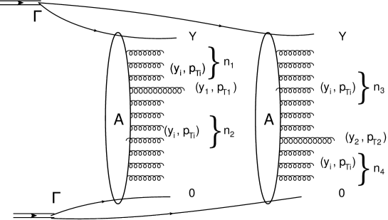
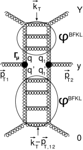
The LRR correlations in CGC/saturation approach originate from the production of two parton showers (see Fig. 1). The double inclusive cross section is described by the Mueller diagram of Fig. 1-b, in which the production of gluons from the parton cascade, is described by the exchange of the BFKL Pomeron (wavy double line in Fig. 1-b), while, due to our poor theoretical knowledge of the confinement of quarks and gluons, the upper and lower blobs in Fig. 1-b require modeling. .

Refer to caption
Figure 1: Production of two gluons with (y1,𝒑T1)subscript𝑦1subscript𝒑𝑇1(y_{1},\boldsymbol{p}_{T1}) and (y2,𝒑T2)subscript𝑦2subscript𝒑𝑇2(y_{2},\boldsymbol{p}_{T2}) in two parton showers (Fig. 1-a). Fig. 1-b shows the double inclusive cross section in the Mueller diagram technique MUDI . The wavy lines denote the BFKL PomeronsBFKL ; LI .

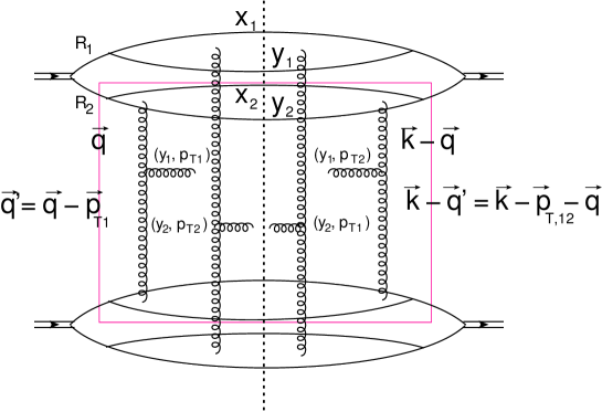
If the two produced gluons have the same quantum numbers, one can see that in addition to the Mueller diagram for different gluons (see Fig. 1-b), we need to take into account a second Mueller diagram of Fig. 2-b, in which two gluons with (y1,𝒑T2)subscript𝑦1subscript𝒑𝑇2(y_{1},\boldsymbol{p}_{T2}) and (y2,𝒑T1)subscript𝑦2subscript𝒑𝑇1(y_{2},\boldsymbol{p}_{T1}) are produced. When 𝒑T1𝒑T2subscript𝒑𝑇1subscript𝒑𝑇2\boldsymbol{p}_{T1}\,\to\,\boldsymbol{p}_{T2}, the two production processes become identical, leading to the cross section σ(two identical gluons)=2σ(two different gluons)𝜎two identical gluons2𝜎two different gluons\sigma\left(\mbox{two identical gluons}\right)=2\sigma\left(\mbox{two different gluons}\right), as one expects. When |𝒑T2𝒑T1|1/Rmuch-greater-thansubscript𝒑𝑇2subscript𝒑𝑇11𝑅|\boldsymbol{p}_{T2}-\boldsymbol{p}_{T1}|\gg 1/R, where R𝑅R is the size of the emitterHBT , the interference diagram becomes small and can be neglected.

The angular correlation emanates from the diagram of Fig. 2-b, in which the upper BFKL Pomerons carry momentum 𝒌𝒑T,12𝒌subscript𝒑𝑇12\boldsymbol{k}-\boldsymbol{p}_{T,12} with 𝒑T,12=𝒑T1𝒑T2subscript𝒑𝑇12subscript𝒑𝑇1subscript𝒑𝑇2\boldsymbol{p}_{T,12}\,=\,\boldsymbol{p}_{T1}\,-\,\boldsymbol{p}_{T2}, while the lower BFKL Pomerons have momenta 𝒌𝒌\boldsymbol{k}. The Mueller diagrams for the correlation between two gluons are shown in Fig. 2.

After integration over kTsubscript𝑘𝑇k_{T}, the sum of diagrams Fig. 2-a and Fig. 2-b can be written as

d2σdy1dy2d2pT1d2pT2(identicalgluons)=d2σdy1dy2d2pT1d2pT2(differentgluons)(1+C(R|𝒑T2𝒑T1|))superscript𝑑2𝜎𝑑subscript𝑦1𝑑subscript𝑦2superscript𝑑2subscript𝑝𝑇1superscript𝑑2subscript𝑝𝑇2identicalgluonssuperscript𝑑2𝜎𝑑subscript𝑦1𝑑subscript𝑦2superscript𝑑2subscript𝑝𝑇1superscript𝑑2subscript𝑝𝑇2differentgluons1𝐶𝑅subscript𝒑𝑇2subscript𝒑𝑇1\frac{d^{2}\sigma}{dy_{1}\,dy_{2}d^{2}p_{T1}d^{2}p_{T2}}\left(\rm identical\,\,gluons\right)\,\,=\,\,\,\frac{d^{2}\sigma}{dy_{1}\,dy_{2}d^{2}p_{T1}d^{2}p_{T2}}\left(\rm different\,\,gluons\right)\Big{(}1\,+\,C\left(R|\boldsymbol{p}_{T2}-\boldsymbol{p}_{T1}|\right)\Big{)} (1)

Eq. (1) coincides with the general formula for the Bose-Einstein correlations HBT ; IPCOR

d2σdy1dy2d2pT1d2pT2(identicalgluons)1+eirμQμproportional-tosuperscript𝑑2𝜎𝑑subscript𝑦1𝑑subscript𝑦2superscript𝑑2subscript𝑝𝑇1superscript𝑑2subscript𝑝𝑇2identicalgluonsdelimited-⟨⟩1superscript𝑒𝑖subscript𝑟𝜇subscript𝑄𝜇\frac{d^{2}\sigma}{dy_{1}\,dy_{2}d^{2}p_{T1}d^{2}p_{T2}}\left(\rm identical\,\,gluons\right)\,\,\propto\,\,\Big{\langle}1\,\,+\,\,e^{ir_{\mu}Q_{\mu}}\Big{\rangle} (2)

where averaging delimited-⟨⟩\langle\dots\rangle includes the integration over rμ=r1,μr2,μsubscript𝑟𝜇subscript𝑟1𝜇subscript𝑟2𝜇r_{\mu}=r_{1,\mu}-r_{2,\mu}. There is only one difference: Qμ=p1.μp2,μsubscript𝑄𝜇subscript𝑝formulae-sequence1𝜇subscript𝑝2𝜇Q_{\mu}=p_{1.\mu}\,-\,p_{2,\mu} degenerates to 𝑸𝒑T,12𝑸subscript𝒑𝑇12\boldsymbol{Q}\,\equiv\,\boldsymbol{p}_{T,12}, due to the fact that the production of two gluons from the two parton showers do not depend on rapidities. Note, that the contribution of Fig. 2-b does not depend on the rapidity difference y1y2subscript𝑦1subscript𝑦2y_{1}-y_{2} nor on y1subscript𝑦1y_{1} and y2subscript𝑦2y_{2}. For y1=y2subscript𝑦1subscript𝑦2y_{1}=y_{2} Eq. (1) follows directly from the general Eq. (2), and the interference diagram of Fig. 3-b leads to Eq. (1), and allows us to calculate the typical correlation radius and the correlation function C(R|𝒑T2𝒑T1|)𝐶𝑅subscript𝒑𝑇2subscript𝒑𝑇1C\left(R|\boldsymbol{p}_{T2}-\boldsymbol{p}_{T1}|\right). On the other hand, for y1y2subscript𝑦1subscript𝑦2y_{1}\neq y_{2} but for 𝒑T1=𝒑T,2subscript𝒑𝑇1subscript𝒑𝑇2\boldsymbol{p}_{T1}=\boldsymbol{p}_{T,2} Eq. (1), gives a constant which does not depend on y1subscript𝑦1y_{1} and y2subscript𝑦2y_{2}. However, in general case y1y2subscript𝑦1subscript𝑦2y_{1}\neq y_{2} and 𝒑T1𝒑T,2subscript𝒑𝑇1subscript𝒑𝑇2\boldsymbol{p}_{T1}\neq\boldsymbol{p}_{T,2} the diagram of Fig. 2-b looks problematic 111We thank Alex Kovner for vigorous discussions on this subject., since it seems to describe the interference between two different final states. In appendix A we demonstrate that the contribution of Fig. 2-b does not vanish even in this general case. Note, that for y1=y2subscript𝑦1subscript𝑦2y_{1}=y_{2}, the sum of two Mueller diagrams , indeed, relates to the interference between two diagrams, as is shown in Fig. 3-a and Fig. 3-b. For these kinematics, as we have mentioned

C(R|𝒑T2𝒑T1|)=ei𝒓T𝑸Twhere𝑸T=𝒑T,12formulae-sequence𝐶𝑅subscript𝒑𝑇2subscript𝒑𝑇1delimited-⟨⟩superscript𝑒𝑖subscript𝒓𝑇subscript𝑸𝑇wheresubscript𝑸𝑇subscript𝒑𝑇12C\left(R|\boldsymbol{p}_{T2}-\boldsymbol{p}_{T1}|\right)\,\,=\,\,\Big{\langle}e^{i\boldsymbol{r}_{T}\cdot\boldsymbol{Q}_{T}}\Big{\rangle}~{}~{}~{}~{}~{}~{}~{}~{}~{}\mbox{where}~{}~{}~{}~{}~{}~{}\boldsymbol{Q}_{T}\,=\,\boldsymbol{p}_{T,12} (3)

For 𝒑T1=𝒑T2subscript𝒑𝑇1subscript𝒑𝑇2\boldsymbol{p}_{T1}=\boldsymbol{p}_{T2}, the sum of two Mueller diagrams can also be viewed as the interference of two diagrams of Fig. 3-c and Fig. 3-d, leading to

C(|0|)=ei𝒓+𝑸+i𝒓𝑸+𝐶0delimited-⟨⟩superscript𝑒𝑖superscript𝒓subscript𝑸𝑖superscript𝒓subscript𝑸C\left(|0|\right)\,\,=\,\,\Big{\langle}e^{i\boldsymbol{r}^{+}\,\boldsymbol{Q}_{-}\,+\,i\boldsymbol{r}^{-}\,\boldsymbol{Q}_{+}}\Big{\rangle} (4)

The calculation of the Mueller diagram shows that this average does not depend on y1subscript𝑦1y_{1} and y2subscript𝑦2y_{2}.

Remembering that for two parton showers in each order of perturbative QCD, (or in other words at fixed multiplicity of the produced gluons) the amplitude can be written in the factorized form A=AL(r+,r)AT(𝒓T)𝐴subscript𝐴𝐿subscript𝑟subscript𝑟subscript𝐴𝑇subscript𝒓𝑇A=A_{L}\left(r_{+},r_{-}\right)\,A_{T}\left(\boldsymbol{r}_{T}\right) leading to

eirμQμ=ei𝒓T𝑸Taveraging over rT×ei𝒓+𝑸+i𝒓𝑸+averaging overr+,rdelimited-⟨⟩superscript𝑒𝑖subscript𝑟𝜇subscript𝑄𝜇subscriptdelimited-⟨⟩superscript𝑒𝑖subscript𝒓𝑇subscript𝑸𝑇averaging over subscript𝑟𝑇subscriptdelimited-⟨⟩superscript𝑒𝑖superscript𝒓subscript𝑸𝑖superscript𝒓subscript𝑸averaging oversubscript𝑟subscript𝑟\Big{\langle}e^{ir_{\mu}\,Q_{\mu}}\Big{\rangle}\,\,=\,\,\,\underbrace{\Big{\langle}e^{i\boldsymbol{r}_{T}\cdot\boldsymbol{Q}_{T}}\Big{\rangle}}_{\mbox{\small averaging over }r_{T}}\times\underbrace{\Big{\langle}e^{i\boldsymbol{r}^{+}\,\boldsymbol{Q}_{-}\,+\,i\boldsymbol{r}^{-}\,\boldsymbol{Q}_{+}}\Big{\rangle}}_{\mbox{\small averaging over}\,r_{+},r_{-}} (5)

In our opinion, the above discussion shows that the Mueller diagram of Fig. 2-b, does not characterize the interference between two orthogonal states, but is an economical way to describe the independence of identical gluon production on rapidities, providing the smooth analytical description of the cross section from y1=y2subscript𝑦1subscript𝑦2y_{1}=y_{2} to the general case y1y2subscript𝑦1subscript𝑦2y_{1}\neq y_{2}. Since this point is not obvious we would like to recall the main features of the leading log(1/x) approximation (LLA). In the LLA we account for the following kinematic regionBFKL ; LI for the production of two parton showers (see Fig. 4):

first parton shower \displaystyle\rightarrow Y>>yi>>yn1>y1>yn2>>yi>>0;𝑌subscript𝑦𝑖subscript𝑦subscript𝑛1subscript𝑦1subscript𝑦subscript𝑛2subscript𝑦𝑖0\displaystyle Y\,>\,\dots\,>\,y_{i}\,>\,\dots\,>\,y_{n_{1}}\,>\,y_{1}\,>\,y_{n_{2}}\,>\,\dots\,>\,y_{i}\,>\,\dots\,>0;
second parton shower \displaystyle\rightarrow Y>>yi>>yn3>y2>yn4>>yi>>0;𝑌subscript𝑦𝑖subscript𝑦subscript𝑛3subscript𝑦2subscript𝑦subscript𝑛4subscript𝑦𝑖0\displaystyle Y\,>\,\dots\,>\,y_{i}\,>\,\dots\,>\,y_{n_{3}}\,>\,y_{2}\,>\,y_{n_{4}}\,>\,\dots\,>\,y_{i}\,>\,\dots\,>0; (6)
parameters of LLA::parameters of LLAabsent\displaystyle\mbox{parameters of LLA}: α¯S 1much-less-thansubscript¯𝛼𝑆1\displaystyle\bar{\alpha}_{S}\,\ll\,1 α¯S(yi+1yi) 1;α¯S(Yyi) 1;α¯S(yi0) 1;α¯S(Yy1) 1;formulae-sequencesubscript¯𝛼𝑆subscript𝑦𝑖1subscript𝑦𝑖1formulae-sequencesubscript¯𝛼𝑆𝑌subscript𝑦𝑖1formulae-sequencesubscript¯𝛼𝑆subscript𝑦𝑖01subscript¯𝛼𝑆𝑌subscript𝑦11\displaystyle\bar{\alpha}_{S}\left(y_{i+1}-y_{i}\right)\,\geq\,1;~{}~{}\bar{\alpha}_{S}\left(Y-y_{i}\right)\,\geq\,1;~{}~{}\bar{\alpha}_{S}\left(y_{i}-0\right)\,\geq\,1;~{}~{}\bar{\alpha}_{S}\left(Y-y_{1}\right)\,\geq\,1;
α¯S(Yy2) 1;α¯S(y10) 1;α¯S(y20) 1;α¯S(y1y2) 1;formulae-sequencesubscript¯𝛼𝑆𝑌subscript𝑦21formulae-sequencesubscript¯𝛼𝑆subscript𝑦101formulae-sequencesubscript¯𝛼𝑆subscript𝑦201subscript¯𝛼𝑆subscript𝑦1subscript𝑦21\displaystyle\bar{\alpha}_{S}\left(Y-y_{2}\right)\,\geq\,1;\bar{\alpha}_{S}\left(y_{1}-0\right)\,\geq\,1;~{}~{}\bar{\alpha}_{S}\left(y_{2}-0\right)\,\geq\,1;~{}~{}\bar{\alpha}_{S}\left(y_{1}-y_{2}\right)\,\geq\,1;

The cross sections of double inclusive productions can be calculated in LLA for the production of two parton showers in the following way:

d2σdifferentgluonsdy1dy2d2pT1d2pT2superscript𝑑2superscript𝜎differentgluons𝑑subscript𝑦1𝑑subscript𝑦2superscript𝑑2subscript𝑝𝑇1superscript𝑑2subscript𝑝𝑇2\displaystyle\frac{d^{2}\sigma^{\rm different\,gluons}}{dy_{1}\,dy_{2}d^{2}p_{T1}d^{2}p_{T2}}\, =\displaystyle= n1+n22>2n3+n42>2𝑑Φn1+n2(1)𝑑Φn3+n4(2)|Adifferentgluons({yi,pTi};y1,pT1;y2,pT2)|2subscriptsuperscriptsubscript𝑛1subscript𝑛222subscriptsuperscriptsubscript𝑛3subscript𝑛422differential-dsubscriptsuperscriptΦ1subscript𝑛1subscript𝑛2differential-dsubscriptsuperscriptΦ2subscript𝑛3subscript𝑛4superscriptsuperscript𝐴differentgluonssubscript𝑦𝑖subscript𝑝𝑇𝑖subscript𝑦1subscript𝑝𝑇1subscript𝑦2subscript𝑝𝑇22\displaystyle\,\,\,\sum^{\infty}_{n_{1}+n_{2}-2>2}\,\,\sum^{\infty}_{n_{3}+n_{4}-2>2}\,\int d\Phi^{(1)}_{n_{1}+n_{2}}d\Phi^{(2)}_{n_{3}+n_{4}}\,|A^{\rm different\,gluons}\left(\{y_{i},p_{Ti}\};y_{1},p_{T1};y_{2},p_{T2}\right)|^{2}
=\displaystyle= n1+n2=n2>2Y>yi>y1n1yi1yi+1𝑑yid2pT,iy1>yi>0n2yi1yi+1𝑑yid2pT,isuperscriptsubscriptsubscript𝑛1subscript𝑛2𝑛22subscriptsuperscriptproductsubscript𝑛1𝑌subscript𝑦𝑖subscript𝑦1subscriptsuperscriptsubscript𝑦𝑖1subscript𝑦𝑖1differential-dsubscript𝑦𝑖superscript𝑑2subscript𝑝𝑇𝑖subscriptsuperscriptproductsubscript𝑛2subscript𝑦1subscript𝑦𝑖0subscriptsuperscriptsubscript𝑦𝑖1subscript𝑦𝑖1differential-dsubscript𝑦𝑖superscript𝑑2subscript𝑝𝑇𝑖\displaystyle\sum_{n_{1}+n_{2}=n-2>2}^{\infty}\,\,\,\,\prod^{n_{1}}_{Y>y_{i}>y_{1}}\int^{y_{i+1}}_{y_{i-1}}dy_{i}d^{2}p_{T,i}\prod^{n_{2}}_{y_{1}>y_{i}>0}\int^{y_{i+1}}_{y_{i-1}}dy_{i}d^{2}p_{T,i}
×\displaystyle\times n3+n4=n2>2Y>yi>y2n3yi1yi+1𝑑yid2pT,iy2>yi>0n4yi1yi+1𝑑yid2pT,isuperscriptsubscriptsubscript𝑛3subscript𝑛4superscript𝑛22subscriptsuperscriptproductsubscript𝑛3𝑌subscript𝑦𝑖subscript𝑦2subscriptsuperscriptsubscript𝑦𝑖1subscript𝑦𝑖1differential-dsubscript𝑦𝑖superscript𝑑2subscript𝑝𝑇𝑖subscriptsuperscriptproductsubscript𝑛4subscript𝑦2subscript𝑦𝑖0subscriptsuperscriptsubscript𝑦𝑖1subscript𝑦𝑖1differential-dsubscript𝑦𝑖superscript𝑑2subscript𝑝𝑇𝑖\displaystyle\,\sum_{n_{3}+n_{4}=n^{\prime}-2>2}^{\infty}\,\,\,\,\prod^{n_{3}}_{Y>y_{i}>y_{2}}\int^{y_{i+1}}_{y_{i-1}}dy_{i}d^{2}p_{T,i}\prod^{n_{4}}_{y_{2}>y_{i}>0}\int^{y_{i+1}}_{y_{i-1}}dy_{i}d^{2}p_{T,i}\,
×\displaystyle\times |Γ2An1n2(2n|{yi,pTi};y1,𝒑T1)An3n4(2n|{yi,pTi};y2,𝒑T2)]2\displaystyle|\Gamma^{2}A_{n_{1}n_{2}}\left(2\to n|\{y_{i},p_{Ti}\};y_{1},\boldsymbol{p}_{T1}\right)A_{n_{3}n_{4}}\left(2\to n|\{y_{i},p_{Ti}\};y_{2},\boldsymbol{p}_{T2}\right)]^{2}
LLALLA\displaystyle\xrightarrow{\rm LLA} n1+n2=n2>2Y>yi>y1n1yi1yi+1𝑑yid2pT,iy1>yi>0n2yi1yi+1𝑑yid2pT,isuperscriptsubscriptsubscript𝑛1subscript𝑛2𝑛22subscriptsuperscriptproductsubscript𝑛1𝑌subscript𝑦𝑖subscript𝑦1subscriptsuperscriptsubscript𝑦𝑖1subscript𝑦𝑖1differential-dsubscript𝑦𝑖superscript𝑑2subscript𝑝𝑇𝑖subscriptsuperscriptproductsubscript𝑛2subscript𝑦1subscript𝑦𝑖0subscriptsuperscriptsubscript𝑦𝑖1subscript𝑦𝑖1differential-dsubscript𝑦𝑖superscript𝑑2subscript𝑝𝑇𝑖\displaystyle\sum_{n_{1}+n_{2}=n-2>2}^{\infty}\,\,\,\,\prod^{n_{1}}_{Y>y_{i}>y_{1}}\int^{y_{i+1}}_{y_{i-1}}dy_{i}d^{2}p_{T,i}\,\,\,\prod^{n_{2}}_{y_{1}>y_{i}>0}\int^{y_{i+1}}_{y_{i-1}}dy_{i}d^{2}p_{T,i}
×\displaystyle\times n3+n4=n2>2Y>yi>y2n3yi1yi+1𝑑yid2pT,iy2>yi>0n4yi1yi+1𝑑yid2pT,isuperscriptsubscriptsubscript𝑛3subscript𝑛4superscript𝑛22subscriptsuperscriptproductsubscript𝑛3𝑌subscript𝑦𝑖subscript𝑦2subscriptsuperscriptsubscript𝑦𝑖1subscript𝑦𝑖1differential-dsubscript𝑦𝑖superscript𝑑2subscript𝑝𝑇𝑖subscriptsuperscriptproductsubscript𝑛4subscript𝑦2subscript𝑦𝑖0subscriptsuperscriptsubscript𝑦𝑖1subscript𝑦𝑖1differential-dsubscript𝑦𝑖superscript𝑑2subscript𝑝𝑇𝑖\displaystyle\,\sum_{n_{3}+n_{4}=n^{\prime}-2>2}^{\infty}\,\,\,\,\prod^{n_{3}}_{Y>y_{i}>y_{2}}\int^{y_{i+1}}_{y_{i-1}}dy_{i}d^{2}p_{T,i}\prod^{n_{4}}_{y_{2}>y_{i}>0}\int^{y_{i+1}}_{y_{i-1}}dy_{i}d^{2}p_{T,i}\,
×\displaystyle\times |Γ2An1n2(2n|{yi=0,pTi};y1=0,𝒑T1)An3n4(2n|{yi=0,pTi};y2=0,𝒑T2)|2\displaystyle|\Gamma^{2}A_{n_{1}n_{2}}\left(2\to n|\{y_{i}=0,p_{Ti}\};y_{1}=0,\boldsymbol{p}_{T1}\right)A_{n_{3}n_{4}}\left(2\to n|\{y_{i}=0,p_{Ti}\};y_{2}=0,\boldsymbol{p}_{T2}\right)|^{2}

where dΦn1+n2(1)𝑑subscriptsuperscriptΦ1subscript𝑛1subscript𝑛2d\Phi^{(1)}_{n_{1}+n_{2}} and dΦn3+n4(2)𝑑subscriptsuperscriptΦ2subscript𝑛3subscript𝑛4d\Phi^{(2)}_{n_{3}+n_{4}} are the phase spaces of the produced gluons in the first and second parton showers. Adifferentgluons({yi,pTi};y1,pT1;y2,pT2)superscript𝐴differentgluonssubscript𝑦𝑖subscript𝑝𝑇𝑖subscript𝑦1subscript𝑝𝑇1subscript𝑦2subscript𝑝𝑇2A^{\rm different\,gluons}\left(\{y_{i},p_{Ti}\};y_{1},p_{T1};y_{2},p_{T2}\right) = Γ2An1n2(2n|{yi,pTi};y1,𝒑T1)An3n4(2n|{yi,pTi};y2,𝒑T2)superscriptΓ2subscript𝐴subscript𝑛1subscript𝑛22conditional𝑛subscript𝑦𝑖subscript𝑝𝑇𝑖subscript𝑦1subscript𝒑𝑇1subscript𝐴subscript𝑛3subscript𝑛42conditional𝑛subscript𝑦𝑖subscript𝑝𝑇𝑖subscript𝑦2subscript𝒑𝑇2\Gamma^{2}A_{n_{1}n_{2}}\left(2\to n|\{y_{i},p_{Ti}\};y_{1},\boldsymbol{p}_{T1}\right)A_{n_{3}n_{4}}\left(2\to n|\{y_{i},p_{Ti}\};y_{2},\boldsymbol{p}_{T2}\right) (see Fig. 4) and all other notations are shown in Fig. 4.

The transition from Eq. (7) to Eq. (7), occurs due to the fact that we want to obtain the log contribution (yi+1yi1)proportional-toabsentsubscript𝑦𝑖1subscript𝑦𝑖1\propto(y_{i+1}-y_{i-1}) for each dyi𝑑subscript𝑦𝑖dy_{i}, These logarithms stem from the integration of the phase space of produced particles, while we can neglect the yisubscript𝑦𝑖y_{i} dependence of the production amplitude. In other words, the production amplitudes are functions only of the transverse momenta and Eq. (7) shows that the longitudinal degrees of freedom can be factorize out BFKL ; LI .

Eq. (7) after integrations over yisubscript𝑦𝑖y_{i}, can be re-written in a more efficacious form , viz.

d2σdy1dy2d2pT1d2pT2superscript𝑑2𝜎𝑑subscript𝑦1𝑑subscript𝑦2superscript𝑑2subscript𝑝𝑇1superscript𝑑2subscript𝑝𝑇2\displaystyle\frac{d^{2}\sigma}{dy_{1}\,dy_{2}d^{2}p_{T1}d^{2}p_{T2}} =\displaystyle= n1+n2=n2>2n1+n2=n2>21n1!(Yy1)n11n2!(y10)n21n3!(Yy2)n31n4!(y20)n4integraloverthelongitudinalphasespacesuperscriptsubscriptsubscript𝑛1subscript𝑛2𝑛22superscriptsubscriptsubscript𝑛1subscript𝑛2superscript𝑛22subscript1subscript𝑛1superscript𝑌subscript𝑦1subscript𝑛11subscript𝑛2superscriptsubscript𝑦10subscript𝑛21subscript𝑛3superscript𝑌subscript𝑦2subscript𝑛31subscript𝑛4superscriptsubscript𝑦20subscript𝑛4integraloverthelongitudinalphasespace\displaystyle\sum_{n_{1}+n_{2}=n-2>2}^{\infty}\,\sum_{n_{1}+n_{2}=n^{\prime}-2>2}^{\infty}\underbrace{\frac{1}{n_{1}!}\left(Y-y_{1}\right)^{n_{1}}\,\frac{1}{n_{2}!}\left(y_{1}-0\right)^{n_{2}\,}\frac{1}{n_{3}!}\left(Y-y_{2}\right)^{n_{3}}\,\frac{1}{n_{4}!}\left(y_{2}-0\right)^{n_{4}}}_{\rm integral\,\,over\,\,the\,longitudinal\,\,phase\,\,space}
×\displaystyle\times id2pTi|Γ2An1n2(2n|{yi=0,pTi};y1=0,𝒑T1)An3n4(2n|{yi=0,pTi};y2=0,𝒑T2)|2\displaystyle\int\prod_{i}d^{2}p_{Ti}\,|\Gamma^{2}A_{n_{1}n_{2}}\left(2\to n|\{y_{i}=0,p_{Ti}\};y_{1}=0,\boldsymbol{p}_{T1}\right)A_{n_{3}n_{4}}\left(2\to n|\{y_{i}=0,p_{Ti}\};y_{2}=0,\boldsymbol{p}_{T2}\right)|^{2}

Summing over nisubscript𝑛𝑖n_{i} we obtain the Mueller diagram of Fig. 1.

For identical particles we need to replace

Adifferentgluons({yi=0,pTi};y1=0,pT1;y2=0,pT2)=\displaystyle A^{\rm different\,gluons}\left(\{y_{i}=0,p_{Ti}\};y_{1}=0,p_{T1};y_{2}=0,p_{T2}\right)\,=
Γ2An1n2(2n|{yi=0,pTi};y1=0,𝒑T1)An3n4(2n|{yi=0,pTi};y2=0,𝒑T2)\displaystyle\Gamma^{2}A_{n_{1}n_{2}}\left(2\to n|\{y_{i}=0,p_{Ti}\};y_{1}=0,\boldsymbol{p}_{T1}\right)A_{n_{3}n_{4}}\left(2\to n|\{y_{i}=0,p_{Ti}\};y_{2}=0,\boldsymbol{p}_{T2}\right)\,\,\to\,\, (9)
Aidenticalgluons({yi=0,pTi};y1=0,pT1;y2=0,pT2)=\displaystyle A^{\rm identical\,gluons}\left(\{y_{i}=0,p_{Ti}\};y_{1}=0,p_{T1};y_{2}=0,p_{T2}\right)\,\,=
Adifferentgluons({0,pTi};y1=0,pT1;y2=0,pT2)+Adifferentgluons({0,pTi};y2=0,pT2;y1=0,pT1)=\displaystyle A^{\rm different\,gluons}\left(\{0,p_{Ti}\};y_{1}=0,p_{T1};y_{2}=0,p_{T2}\right)\,+\,A^{\rm different\,gluons}\left(\{0,p_{Ti}\};y_{2}=0,p_{T2};y_{1}=0,p_{T1}\right)\,=
Γ2An1,n2(2n|{yi=0,pTi};y1=0,𝒑T1)An3n4(2n|{yi=0,pTi};y2=0,𝒑T2)\displaystyle\hskip 85.35826pt\Gamma^{2}A_{n_{1},n_{2}}\left(2\to n|\{y_{i}=0,p_{Ti}\};y_{1}=0,\boldsymbol{p}_{T1}\right)A_{n_{3}n_{4}}\left(2\to n|\{y_{i}=0,p_{Ti}\};y_{2}=0,\boldsymbol{p}_{T2}\right)\,\,
+Γ2An1n2(2n|{yi=0,pTi};y2=0,𝒑T2)An3n4(2n|{yi=0,pTi};y1=0,𝒑T1)\displaystyle\hskip 85.35826pt+\,\,\Gamma^{2}A_{n_{1}n_{2}}\left(2\to n|\{y_{i}=0,p_{Ti}\};y_{2}=0,\boldsymbol{p}_{T2}\right)A_{n_{3}n_{4}}\left(2\to n|\{y_{i}=0,p_{Ti}\};y_{1}=0,\boldsymbol{p}_{T1}\right)

We wish to stress, that in Eq. (I) we use the Bose-Einstein symmetry for the production amplitudes, which are only functions of the transverse momenta of produced particles.

Such a replacement leads to the sum of the diagrams of Fig. 2-a and Fig. 2-b.

The goal of this paper is to calculate the function C(R|𝒑T2𝒑T1|)𝐶𝑅subscript𝒑𝑇2subscript𝒑𝑇1\,C\left(R|\boldsymbol{p}_{T2}-\boldsymbol{p}_{T1}|\right) which tends to 1 at 𝒑T2𝒑T1subscript𝒑𝑇2subscript𝒑𝑇1\boldsymbol{p}_{T2}\to\boldsymbol{p}_{T1}, and vanishes for R|𝒑T2𝒑T1| 1much-greater-than𝑅subscript𝒑𝑇2subscript𝒑𝑇11R|\boldsymbol{p}_{T2}-\boldsymbol{p}_{T1}|\,\gg\,1. To estimate C(R|𝒑T2𝒑T1|)𝐶𝑅subscript𝒑𝑇2subscript𝒑𝑇1C\left(R|\boldsymbol{p}_{T2}-\boldsymbol{p}_{T1}|\right), it is sufficient to know the double inclusive cross section for y1=y2subscript𝑦1subscript𝑦2y_{1}=y_{2} , where Fig. 2-b contributes significantly.

Refer to caption
Figure 2: Production of two identical gluons with (y1,𝒑T1)subscript𝑦1subscript𝒑𝑇1(y_{1},\boldsymbol{p}_{T1}) and (y2,𝒑T2)subscript𝑦2subscript𝒑𝑇2(y_{2},\boldsymbol{p}_{T2}) in two parton showers. The diagrams in the Mueller diagram technique MUDI are shown in Fig. 2-a and Fig. 2-b. The wavy lines denote the BFKL PomeronsBFKL ; LI .

To obtain the double inclusive cross section, we need to add the cross section for two different gluon production which has the form

d2σdy1dy2d2pT1d2pT2=d2σdy1dy2d2pT1d2pT2(differentgluons)(1+1Nc21C(R|𝒑T2𝒑T1|))superscript𝑑2𝜎𝑑subscript𝑦1𝑑subscript𝑦2superscript𝑑2subscript𝑝𝑇1superscript𝑑2subscript𝑝𝑇2superscript𝑑2𝜎𝑑subscript𝑦1𝑑subscript𝑦2superscript𝑑2subscript𝑝𝑇1superscript𝑑2subscript𝑝𝑇2differentgluons11subscriptsuperscript𝑁2𝑐1𝐶𝑅subscript𝒑𝑇2subscript𝒑𝑇1\frac{d^{2}\sigma}{dy_{1}\,dy_{2}d^{2}p_{T1}d^{2}p_{T2}}\,\,=\,\,\frac{d^{2}\sigma}{dy_{1}\,dy_{2}d^{2}p_{T1}d^{2}p_{T2}}\left(\rm different\,\,gluons\right)\Bigg{(}1\,+\,\frac{1}{N^{2}_{c}-1}\,\,C\left(R|\boldsymbol{p}_{T2}-\boldsymbol{p}_{T1}|\right)\Bigg{)} (10)

In Eq. (10) we take into account, that we have Nc21subscriptsuperscript𝑁2𝑐1N^{2}_{c}-1 pairs of the identical gluons, where Ncsubscript𝑁𝑐N_{c} is the number of colours, and that the polarizations of the identical gluons should be the same. The latter leads to a suppression of 1212\frac{1}{2} of the second term in Eq. (10). Using Eq. (10) we can find vnsubscript𝑣𝑛v_{n}, since

d2σdy1dy2d2pT1d2pT2  1+  2nVnΔ(pT1,pT2)cos(Δφ)proportional-tosuperscript𝑑2𝜎𝑑subscript𝑦1𝑑subscript𝑦2superscript𝑑2subscript𝑝𝑇1superscript𝑑2subscript𝑝𝑇212subscript𝑛subscript𝑉𝑛Δsubscript𝑝𝑇1subscript𝑝𝑇2Δ𝜑\frac{d^{2}\sigma}{dy_{1}\,dy_{2}d^{2}p_{T1}d^{2}p_{T2}}\,\,\propto\,\,1\,\,+\,\,2\sum_{n}V_{n\Delta}\left(p_{T1},p_{T2}\right)\,\cos\left(\Delta\,\varphi\right) (11)

where ΔφΔ𝜑\Delta\varphi is the angle between 𝒑T1subscript𝒑𝑇1\boldsymbol{p}_{T1} and 𝒑T2subscript𝒑𝑇2\boldsymbol{p}_{T2}. vnsubscript𝑣𝑛v_{n} is determined from VnΔ(pT1,pT2)subscript𝑉𝑛Δsubscript𝑝𝑇1subscript𝑝𝑇2V_{n\Delta}\left(p_{T1},p_{T2}\right)

1.vn(pT)=VnΔ(pT,pT);2.vn(pT)=VnΔ(pT,pTRef)VnΔ(pTRef,pTRef);1.~{}~{}v_{n}\left(p_{T}\right)\,\,=\,\,\sqrt{V_{n\Delta}\left(p_{T},p_{T}\right)}\,;\,~{}~{}~{}~{}~{}~{}~{}~{}~{}~{}~{}~{}~{}2.~{}~{}~{}~{}v_{n}\left(p_{T}\right)\,\,=\,\,\frac{V_{n\Delta}\left(p_{T},p^{\rm Ref}_{T}\right)}{\sqrt{V_{n\Delta}\left(p^{\rm Ref}_{T},p^{\rm Ref}_{T}\right)}}\,; (12)

Eq. (12)-1 and Eq. (12)-2 depict two methods of how the values of vnsubscript𝑣𝑛v_{n} have been extracted from the experimentally measured VnΔ(pT1,pT2)subscript𝑉𝑛Δsubscript𝑝𝑇1subscript𝑝𝑇2V_{n\Delta}\left(p_{T1},p_{T2}\right). pTRefsubscriptsuperscript𝑝Ref𝑇p^{\rm Ref}_{T} denotes the momentum of the reference trigger. These two definitions are equivalent if VnΔ(pT1,pT2)subscript𝑉𝑛Δsubscript𝑝𝑇1subscript𝑝𝑇2V_{n\Delta}\left(p_{T1},p_{T2}\right) can be factorized as VnΔ(pT1,pT2)=vn(pT1)vn(pT2)subscript𝑉𝑛Δsubscript𝑝𝑇1subscript𝑝𝑇2subscript𝑣𝑛subscript𝑝𝑇1subscript𝑣𝑛subscript𝑝𝑇2V_{n\Delta}\left(p_{T1},p_{T2}\right)\,=\,v_{n}\left(p_{T1}\right)\,v_{n}\left(p_{T2}\right). We will show below that in our approach this is the case for the restricted kinematic region RpTi 1much-less-than𝑅subscript𝑝𝑇𝑖1R\,p_{Ti}\,\ll\,1.

Refer to caption
Figure 3: The interferences between two states for the production of two identical gluons in two specific cases: y1=y2subscript𝑦1subscript𝑦2y_{1}=y_{2} (Fig. 3-a and Fig. 3 -b) and 𝒑T1=𝒑T2subscript𝒑𝑇1subscript𝒑𝑇2\boldsymbol{p}_{T1}=\boldsymbol{p}_{T2}(Fig. 3-c and Fig. 3 -d).

The first problem that we face in calculating C(R|𝒑T2𝒑T1|)𝐶𝑅subscript𝒑𝑇2subscript𝒑𝑇1C\left(R|\boldsymbol{p}_{T2}-\boldsymbol{p}_{T1}|\right), is to estimate the value of R𝑅R, which increases with energy (see for example LHC data of Ref.TOTEM ). On the other hand, the BFKL PomeronBFKL ; LI does not lead to the shrinkage of the diffraction peak, as it has no slope for the Pomeron trajectory. The only way to obtain a size which increases with energy, is to use the unitarity constraints , ABFKL(Y,b)eΔBFKLYa(b)< 1proportional-tosuperscript𝐴BFKL𝑌𝑏superscript𝑒subscriptΔBFKL𝑌𝑎𝑏1A^{\rm BFKL}\left(Y,b\right)\propto e^{\Delta_{\rm BFKL}\,Y}a(b)\,<\,1 FROI , where ΔBFKLsubscriptΔBFKL\Delta_{\rm BFKL} is the intercept of the BFKL Pomeron and b𝑏b is the impact factor. However, in QCD a(b)𝑎𝑏a\left(b\right) decreases as a power of b𝑏b and the unitarity constraints lead to Rexp(ΔBFKLY)proportional-to𝑅subscriptΔBFKL𝑌R\,\,\propto\,\,\exp\left(\Delta_{\rm BFKL}\,Y\right) KOWE . Therefore, to obtain the energy behaviour of R𝑅R, we need to introduce a non-perturbative correction at large b𝑏b, which assures a(b)exp(μsoftb)proportional-to𝑎𝑏subscript𝜇soft𝑏a(b)\,\,\propto\,\exp\left(-\mu_{\rm soft}b\right), and also to take into account the multi Pomeron interactions which satisfy the unitarity constraints. Fortunately, the second part of the problem has been solved in the CGC/saturation approachKOLEB , but the first needs modelling of the unknown confinement of quarks and gluons. Hence, we are doomed to build a model which includes everything that we know theoretically regarding the CGC/saturation approach, but in addition, one needs to introduce some phenomenological descriptions of the hadron structure, and the large b𝑏b behaviour of the BFKL Pomeron.

Refer to caption
Figure 4: The amplitude of production of n=n1+n2+n3+n4𝑛subscript𝑛1subscript𝑛2subscript𝑛3subscript𝑛4n=n_{1}+n_{2}+n_{3}+n_{4} particles, Adifferentgluons(2n|{yi,pTi};y1,𝒑T1;y2,𝒑T2)superscript𝐴differentgluons2conditional𝑛subscript𝑦𝑖subscript𝑝𝑇𝑖subscript𝑦1subscript𝒑𝑇1subscript𝑦2subscript𝒑𝑇2A^{\rm different\,gluons}\left(2\to n|\{y_{i},p_{Ti}\};y_{1},\boldsymbol{p}_{T1};y_{2},\boldsymbol{p}_{T2}\right) (see Eq. (7))

Such a model for hadron-hadron interactions at high energy has been developed in Refs.GLM2CH ; GLMNI ; GLMINCL ; GLMCOR , and it successfully describes the experimental data on total, inelastic and diffractive cross sections, as well as the inclusive production and LRR correlations. The goal of this paper is to show that the structure of the ‘dressed’ Pomeron in this model leads to strong BE correlations, and generates vnsubscript𝑣𝑛v_{n} both for even and odd n𝑛n, in hadron and nucleus interactions. In the next section we consider the contribution to C(R|𝒑T2𝒑T1|)𝐶𝑅subscript𝒑𝑇2subscript𝒑𝑇1C\left(R|\boldsymbol{p}_{T2}-\boldsymbol{p}_{T1}|\right) from the first Mueller diagram, and discuss the different sources of BE-correlations. In section 3 we give a brief review of the structure of the Pomeron in our model, in which we incorporate the solution to the CGC/saturation equations with additional non-perturbative assumptions: the large b𝑏b behaviour for the saturation momentum, and the structure of hadrons. It has been known for a long time OLDREG ; PION in the framework of Gribov Pomeron calculus, and has been re-considered in CGC/saturation approach RIDGE , that the LRR correlations stem from the production of gluon jets from two different parton showers (see Fig. 1). In section 4 we evaluate the BE correlations that result from the dressed Pomeron of our model, and show that they are able to describe the main features of the experimental data.

II Calculation of the first diagram

II.1 Proton-proton scattering

The first Mueller diagram which contributes to C(R|𝒑T2𝒑T1|)𝐶𝑅subscript𝒑𝑇2subscript𝒑𝑇1C\left(R|\boldsymbol{p}_{T2}-\boldsymbol{p}_{T1}|\right) and which we need to calculate, is shown in Fig. 2-e and can be written in the form LERE :

d2σdy1dy2d2pT1d2pT2=d2σdy1dy2d2pT1d2pT2(differentgluons)(1Nc21C(R|𝒑T2𝒑T1|))superscript𝑑2𝜎𝑑subscript𝑦1𝑑subscript𝑦2superscript𝑑2subscript𝑝𝑇1superscript𝑑2subscript𝑝𝑇2superscript𝑑2𝜎𝑑subscript𝑦1𝑑subscript𝑦2superscript𝑑2subscript𝑝𝑇1superscript𝑑2subscript𝑝𝑇2differentgluons1subscriptsuperscript𝑁2𝑐1𝐶𝑅subscript𝒑𝑇2subscript𝒑𝑇1\displaystyle\frac{d^{2}\sigma}{dy_{1}\,dy_{2}d^{2}p_{T1}d^{2}p_{T2}}\,\,=\,\,\frac{d^{2}\sigma}{dy_{1}\,dy_{2}d^{2}p_{T1}d^{2}p_{T2}}\left(\rm different\,\,gluons\right)\Bigg{(}\frac{1}{N^{2}_{c}-1}\,\,C\left(R|\boldsymbol{p}_{T2}-\boldsymbol{p}_{T1}|\right)\Bigg{)} (13)
=(α¯SCF2π)2d2kTNIPh(kT2)NIPh((𝒌𝑻+𝒑T,12)2)dσdy1d2pT1(kT,|𝒌𝑻+𝒑T,12|)dσdy2d2pT2(kT,|𝒌𝑻+𝒑T,12|)absentsuperscriptsubscript¯𝛼𝑆subscript𝐶𝐹2𝜋2superscript𝑑2subscript𝑘𝑇subscript𝑁𝐼𝑃subscriptsuperscript𝑘2𝑇subscript𝑁𝐼𝑃superscriptsubscript𝒌𝑻subscript𝒑𝑇122𝑑𝜎𝑑subscript𝑦1superscript𝑑2subscript𝑝𝑇1subscript𝑘𝑇subscript𝒌𝑻subscript𝒑𝑇12𝑑𝜎𝑑subscript𝑦2superscript𝑑2subscript𝑝𝑇2subscript𝑘𝑇subscript𝒌𝑻subscript𝒑𝑇12\displaystyle=\,\left(\frac{\bar{\alpha}_{S}\,C_{F}}{2\pi}\right)^{2}\int d^{2}k_{T}\,N_{{I\!\!P}h}\left(k^{2}_{T}\right)\,N_{{I\!\!P}h}\left(\left(\ \boldsymbol{k_{T}}+\boldsymbol{p}_{T,12}\right)^{2}\right)\,\frac{d\sigma}{dy_{1}d^{2}p_{T1}}\left(k_{T},|\boldsymbol{k_{T}}+\boldsymbol{p}_{T,12}|\right)\frac{d\sigma}{dy_{2}d^{2}p_{T2}}\left(k_{T},|\boldsymbol{k_{T}}+\boldsymbol{p}_{T,12}|\right)

where 𝒑T,12=𝒑T1𝒑T2subscript𝒑𝑇12subscript𝒑𝑇1subscript𝒑𝑇2\boldsymbol{p}_{T,12}=\boldsymbol{p}_{T1}\,-\,\boldsymbol{p}_{T2} and

dσdy1d2pT1(kT,|𝒌𝑻+𝒑T,12|)=𝑑𝜎𝑑subscript𝑦1superscript𝑑2subscript𝑝𝑇1subscript𝑘𝑇subscript𝒌𝑻subscript𝒑𝑇12absent\displaystyle\frac{d\sigma}{dy_{1}d^{2}p_{T1}}\left(k_{T},|\boldsymbol{k_{T}}+\boldsymbol{p}_{T,12}|\right)\,= (14)
d2qTϕBFKL(qT,𝒌T𝒒T)Γμ(qT,pT1)Γμ(𝒌T𝒒T,pT2)ϕBFKL(qT,𝒌T+𝒑T,12𝒒T)superscript𝑑2subscript𝑞𝑇superscriptitalic-ϕBFKLsubscript𝑞𝑇subscript𝒌𝑇subscript𝒒𝑇subscriptΓ𝜇subscript𝑞𝑇subscript𝑝𝑇1subscriptΓ𝜇subscript𝒌𝑇subscript𝒒𝑇subscript𝑝𝑇2superscriptitalic-ϕBFKLsubscript𝑞𝑇subscript𝒌𝑇subscript𝒑𝑇12subscript𝒒𝑇\displaystyle\,\int d^{2}q_{T}\,\phi^{\rm BFKL}\left(q_{T},\boldsymbol{k}_{T}-\boldsymbol{q}_{T}\right)\,\Gamma_{\mu}\left(q_{T},p_{T1}\right)\,\Gamma_{\mu}\left(\boldsymbol{k}_{T}-\boldsymbol{q}_{T},p_{T2}\right)\,\phi^{\rm BFKL}\left(q_{T},\boldsymbol{k}_{T}+\boldsymbol{p}_{T,12}-\boldsymbol{q}_{T}\right)

In Eq. (14) ϕBFKLsuperscriptitalic-ϕBFKL\phi^{\rm BFKL} denotes the parton density of the BFKL Pomeron, with momentum transferred by the Pomeron 𝒌Tsubscript𝒌𝑇\boldsymbol{k}_{T} or 𝒌T+𝒑T,12subscript𝒌𝑇subscript𝒑𝑇12\boldsymbol{k}_{T}+\boldsymbol{p}_{T,12}. The Lipatov vertex ΓμsubscriptΓ𝜇\Gamma_{\mu}, as well as the equations for ϕBFKLsuperscriptitalic-ϕBFKL\phi^{\rm BFKL} will be discussed in the appendix A. Generally speaking, NIPhsubscript𝑁𝐼𝑃N_{{I\!\!P}h} has a structure which is shown in Fig. 5:

NIPh(kT2)=MnM0gIPn2(kT2)δ(M2Mn2)+gIPh(0)G3IP(kT2)eΔBFKLYsubscript𝑁𝐼𝑃subscriptsuperscript𝑘2𝑇subscriptsuperscriptsubscript𝑀0subscript𝑀𝑛subscriptsuperscript𝑔2𝐼𝑃𝑛subscriptsuperscript𝑘2𝑇𝛿superscript𝑀2subscriptsuperscript𝑀2𝑛subscript𝑔𝐼𝑃0subscript𝐺3𝐼𝑃subscriptsuperscript𝑘2𝑇superscript𝑒subscriptΔBFKL𝑌N_{{I\!\!P}h}\left(k^{2}_{T}\right)\,\,=\,\,\sum^{M_{0}}_{M_{n}}\,g^{2}_{{I\!\!P}n}\left(k^{2}_{T}\right)\delta\left(M^{2}-M^{2}_{n}\right)\,+\,g_{{I\!\!P}h}\left(0\right)\,G_{3{I\!\!P}}\left(k^{2}_{T}\right)\,e^{\Delta_{\rm BFKL}Y} (15)

where Mnsubscript𝑀𝑛M_{n} denotes the mass of resonances, ΔBFKLsubscriptΔBFKL\Delta_{\rm BFKL} the intercept of the BFKL Pomeron, and G3IPsubscript𝐺3𝐼𝑃G_{3{I\!\!P}} the triple Pomeron vertex. Considering the contribution of the first term to NIPhsubscript𝑁𝐼𝑃N_{{I\!\!P}h}, we can neglect, in the first approximation, the dependence of ϕBFKLsuperscriptitalic-ϕBFKL\phi^{\rm BFKL} on the momentum transferred, since QTsubscript𝑄𝑇Q_{T} turns out to be of the order of the saturation momentum Qs 1/Rhmuch-greater-thansubscript𝑄𝑠1subscript𝑅Q_{s}\,\gg\,1/R_{h}, where Rhsubscript𝑅R_{h} is the hadron size incorporated in NIPhsubscript𝑁𝐼𝑃N_{{I\!\!P}h}.

Refer to caption
Figure 5: The structure of NIPh(kT2)subscript𝑁𝐼𝑃subscriptsuperscript𝑘2𝑇N_{{I\!\!P}h}\left(k^{2}_{T}\right).

This is not the case for the second term in Eq. (15), which has QTQssimilar-tosubscript𝑄𝑇subscript𝑄𝑠Q_{T}\sim Q_{s}. It leads to the BFKL Pomeron calculus which takes the Pomeron interactions into account. We will discuss this contribution in sections 3 and 4. In this section we restrict ourselves to the first term in the sum in Eq. (5). Collecting all formulae, we obtain that in the first diagram

C(R|𝒑T2𝒑T1|)d2kTgIP,pr2(kT2)gIP,tr2((𝒌𝒑T,12)2)/d2kTgIP,pr2(kT2)gIP,tr2(kT2)proportional-to𝐶𝑅subscript𝒑𝑇2subscript𝒑𝑇1superscript𝑑2subscript𝑘𝑇subscriptsuperscript𝑔2𝐼𝑃prsubscriptsuperscript𝑘2𝑇subscriptsuperscript𝑔2𝐼𝑃trsuperscript𝒌subscript𝒑𝑇122superscript𝑑2subscript𝑘𝑇subscriptsuperscript𝑔2𝐼𝑃prsubscriptsuperscript𝑘2𝑇subscriptsuperscript𝑔2𝐼𝑃trsubscriptsuperscript𝑘2𝑇C\left(R|\boldsymbol{p}_{T2}-\boldsymbol{p}_{T1}|\right)\,\,\propto\,\,\int d^{2}k_{T}\,g^{2}_{{I\!\!P},{\rm pr}}\left(k^{2}_{T}\right)\,g^{2}_{{I\!\!P},{\rm tr}}\left(\left(\boldsymbol{k}-\boldsymbol{p}_{T,12}\right)^{2}\right)\Bigg{/}\int d^{2}k_{T}\,g^{2}_{{I\!\!P},{\rm pr}}\left(k^{2}_{T}\right)\,g^{2}_{{I\!\!P},{\rm tr}}\left(k^{2}_{T}\right) (16)

To obtain the first estimates for the vertices of the soft Pomeron interaction with the projectile and target, we use the following parameterizations:

gpr(k2)=gpr0e12BprkT2;gtr(k2)=gtr0e12BtrkT2;formulae-sequencesubscript𝑔𝑝𝑟superscript𝑘2subscriptsuperscript𝑔0𝑝𝑟superscript𝑒12subscript𝐵𝑝𝑟subscriptsuperscript𝑘2𝑇subscript𝑔𝑡𝑟superscript𝑘2subscriptsuperscript𝑔0𝑡𝑟superscript𝑒12subscript𝐵𝑡𝑟subscriptsuperscript𝑘2𝑇g_{pr}\left(k^{2}\right)\,=\,g^{0}_{pr}\,e^{-\frac{1}{2}B_{pr}\,k^{2}_{T}};~{}~{}~{}~{}~{}~{}~{}~{}g_{tr}\left(k^{2}\right)\,=\,g^{0}_{tr}\,e^{-\frac{1}{2}B_{tr}\,k^{2}_{T}}; (17)

For proton-proton collisions we take Bpr=Btr=Bsubscript𝐵𝑝𝑟subscript𝐵𝑡𝑟𝐵B_{pr}=B_{tr}=B.

In this case GLMBE ; PION

C(R|𝒑T2𝒑T1|)=exp(BR(pT122pT1pT2cos(Δφ)+pT22))𝐶𝑅subscript𝒑𝑇2subscript𝒑𝑇1subscript𝐵𝑅subscriptsuperscript𝑝2𝑇12subscript𝑝𝑇1subscript𝑝𝑇2Δ𝜑subscriptsuperscript𝑝2𝑇2C\left(R|\boldsymbol{p}_{T2}-\boldsymbol{p}_{T1}|\right)\,\,=\,\,\exp\left(-B_{R}\,\left(p^{2}_{T1}-2p_{T1}p_{T2}\cos\left(\Delta\varphi\right)\,+\,p^{2}_{T2}\right)\right) (18)

with BR=BprBtr/(Bpr+Btr)subscript𝐵𝑅subscript𝐵𝑝𝑟subscript𝐵𝑡𝑟subscript𝐵𝑝𝑟subscript𝐵𝑡𝑟B_{R}=B_{pr}B_{tr}/\left(B_{pr}\,+\,B_{tr}\right). BR=12Bsubscript𝐵𝑅12𝐵B_{R}=\frac{1}{2}B for proton-proton scattering.

In Ref.GLMBE it is shown that Eq. (18) leads to VΔnsubscript𝑉Δ𝑛V_{\Delta n} of Eq. (11) which is equal to

VΔn=In(2BRpT1pT2)eBR(pT12+pT22)NC21+I0(2BRpT1pT2)eBR(pT12+pT22)subscript𝑉Δ𝑛subscript𝐼𝑛2subscript𝐵𝑅subscript𝑝𝑇1subscript𝑝𝑇2superscript𝑒subscript𝐵𝑅subscriptsuperscript𝑝2𝑇1subscriptsuperscript𝑝2𝑇2subscriptsuperscript𝑁2𝐶1subscript𝐼02subscript𝐵𝑅subscript𝑝𝑇1subscript𝑝𝑇2superscript𝑒subscript𝐵𝑅subscriptsuperscript𝑝2𝑇1subscriptsuperscript𝑝2𝑇2V_{\Delta\,n}\,\,=\,\,\ I_{n}\left(2B_{R}p_{T1}p_{T2}\right)\frac{e^{-B_{R}\left(p^{2}_{T1}\,+\,p^{2}_{T2}\right)}}{N^{2}_{C}-1\,\,+\,\,I_{0}\left(2B_{R}p_{T1}p_{T2}\right)\,e^{-B_{R}\left(p^{2}_{T1}\,+\,p^{2}_{T2}\right)}} (19)

where Insubscript𝐼𝑛I_{n} is the modified Bessel function of the first kind.

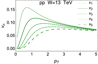
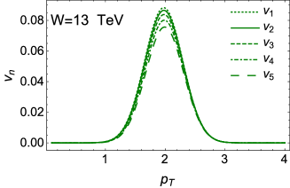
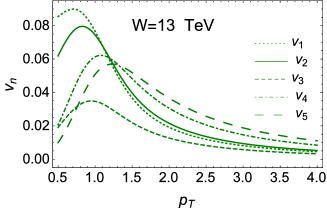
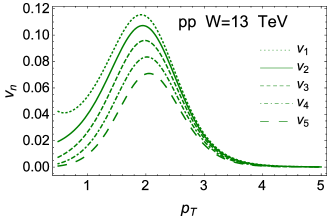
In Fig. 6 taking BR=5GeV2subscript𝐵𝑅5𝐺𝑒superscript𝑉2B_{R}=5\,GeV^{-2}, we plot the prediction for vnsubscript𝑣𝑛v_{n} using Eq. (19) and Eq. (12). This value of BRsubscript𝐵𝑅B_{R}, corresponds to the slope of the elastic cross section for proton-proton scattering at W=13GeV𝑊13𝐺𝑒𝑉W=13\,GeV. One can see that Eq. (12)-1 and Eq. (12)-2 give different predictions, demonstrating that we do not have factorization VnΔ(pT1,pT2)vn(pT1)vn(pT2)subscript𝑉𝑛Δsubscript𝑝𝑇1subscript𝑝𝑇2subscript𝑣𝑛subscript𝑝𝑇1subscript𝑣𝑛subscript𝑝𝑇2V_{n\Delta}\left(p_{T1},p_{T2}\right)\,\neq\,v_{n}\left(p_{T1}\right)\,v_{n}\left(p_{T2}\right). Fig. 6-c shows vnsubscript𝑣𝑛v_{n} for pTminpT2=pTRefpTmaxsubscriptsuperscript𝑝min𝑇subscript𝑝𝑇2subscriptsuperscript𝑝Ref𝑇subscriptsuperscript𝑝max𝑇p^{\rm min}_{T}\leq p_{T2}=p^{\rm Ref}_{T}\leq p^{\rm max}_{T} with pTmin=0.5GeVsubscriptsuperscript𝑝min𝑇0.5𝐺𝑒𝑉p^{\rm min}_{T}=0.5\,GeV and pTmax=5GeVsubscriptsuperscript𝑝max𝑇5𝐺𝑒𝑉p^{\rm max}_{T}=5\,GeV, as done in Ref.ATLASPP . To calculate such a vnsubscript𝑣𝑛v_{n}, we need to know the dependence of the cross section on pT2subscript𝑝𝑇2p_{T2}. Indeed, we need to take Eq. (10) and integrate it over pT2subscript𝑝𝑇2p_{T2}: viz.

H(pT1,Δφ)=pT2minpT2maxdpT22d2σdy1dy2d2pT1d2pT2(Eq.(10))  1+  2nVnΔ(pT1)cos(Δφ)H\left(p_{T1},\Delta\varphi\right)\,=\,\int^{p^{\rm max}_{T2}}_{p^{\rm min}_{T2}}dp^{2}_{T2}\,\frac{d^{2}\sigma}{dy_{1}\,dy_{2}d^{2}p_{T1}d^{2}p_{T2}}\left({Eq.~{}(\ref{I2})}\right)\,\,\propto\,\,1\,\,+\,\,2\sum_{n}V_{n\Delta}\left(p_{T1}\right)\,\cos\left(\Delta\,\varphi\right) (20)

For Fig. 6-c, we need to know the behaviour of the double inclusive cross section on pT1subscript𝑝𝑇1p_{T1} and pT2subscript𝑝𝑇2p_{T2}. We assume that d2σdy1dy2d2pT1d2pT2 1/(pT12pT22)proportional-tosuperscript𝑑2𝜎𝑑subscript𝑦1𝑑subscript𝑦2superscript𝑑2subscript𝑝𝑇1superscript𝑑2subscript𝑝𝑇21subscriptsuperscript𝑝2𝑇1subscriptsuperscript𝑝2𝑇2\frac{d^{2}\sigma}{dy_{1}\,dy_{2}\,d^{2}p_{T1}d^{2}p_{T2}}\,\propto\,1\Big{/}\left(p^{2}_{T1}\,p^{2}_{T2}\right) for the cross sections given by Fig. 1-b and by Fig. 2-c and Fig. 2-d. In the appendix A we show that the cross section for Fig. 2-e d2σdy1dy2d2pT1d2pT2(Fig.2e)(1/pT12+ 1/pT22)2\frac{d^{2}\sigma}{dy_{1}\,dy_{2}\,d^{2}p_{T1}d^{2}p_{T2}}\left({Fig.~{}\ref{2shiden}}-e\right)\,\propto\,\Big{(}1/p^{2}_{T1}\,+\,1/p^{2}_{T2}\Big{)}^{2}.

Refer to caption Refer to caption Refer to caption
Fig. 6-a Fig. 6-b Fig. 6-c
Figure 6: vnsubscript𝑣𝑛v_{n} versus pTsubscript𝑝𝑇p_{T} for proton-proton scattering at W=13TeV𝑊13𝑇𝑒𝑉W=13\,TeV, using Eq. (19) and Eq. (12). Fig. 6-a shows vnsubscript𝑣𝑛v_{n} that stem from Eq. (12)-1. In Fig. 6-b the estimates from Eq. (12)-2 for pTRef=2GeVsubscriptsuperscript𝑝Ref𝑇2𝐺𝑒𝑉p^{\rm Ref}_{T}=2\,GeV are plotted. Fig. 6-c describes the same vnsubscript𝑣𝑛v_{n} as in Fig. 6-b, where, pTRefsubscriptsuperscript𝑝Ref𝑇p^{\rm Ref}_{T} is taken in the interval 0.55GeV0.55𝐺𝑒𝑉0.5-5\,GeV, as is measured in Ref.ATLASPP .

We took the energy dependence into account, by calculating the BRsubscript𝐵𝑅B_{R} from the slope of the elastic scattering at given energy W𝑊W, which was taken from Ref.GLM2CH .

Refer to caption Refer to caption
Fig. 7-a Fig. 7-b
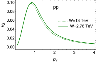
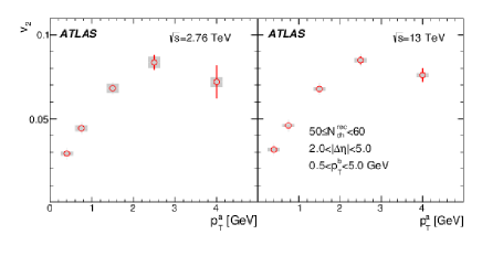
Figure 7: v2subscript𝑣2v_{2} versus pTsubscript𝑝𝑇p_{T} for proton-proton scattering at W= 2.76TeV𝑊2.76𝑇𝑒𝑉W\,=\,2.76\,TeV and at W= 13TeV𝑊13𝑇𝑒𝑉W\,=\,13\,TeV. Fig. 7-a shows vnsubscript𝑣𝑛v_{n} that stem from Eq. (12)-2 for pTRefsubscriptsuperscript𝑝Ref𝑇p^{\rm Ref}_{T} which is taken in the interval 0.5 to 5 GeV, as is measured in Ref.ATLASPP . Fig. 7-b exhibits the experimental data taken from Ref.ATLASPP .

One can see that the calculated values, as well as energy dependence are close to the experimental data of Ref.ATLASPP . The main difference is in the pTsubscript𝑝𝑇p_{T} dependence, which suggests the necessity to include the diffractive dissociation process or, in other words, the entire sum in Eq. (15), as well as the enhanced diagrams that are generated by the BFKL Pomeron calculus (see Fig. 5).

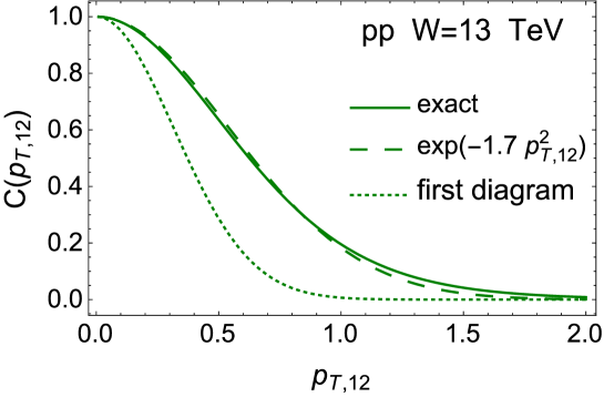
We can estimate the sum over resonances or, in other words, the diffraction production of states with low mass, by using our model (see appendix B for necessary formulae). In Fig. 8 we plot the correlation function C(pT,12)𝐶subscript𝑝𝑇12C\left(p_{T,12}\right) as defined in Eq. (10) for |𝒑T1|=|𝒑T2|subscript𝒑𝑇1subscript𝒑𝑇2|\boldsymbol{p}_{T1}|=|\boldsymbol{p}_{T2}|, which is the result of these calculations. One can see that the effective pT,12subscript𝑝𝑇12p_{T,12} dependence of the slope, turns out to be much smaller than our estimates from the first diagrams that we obtained above. The slope that we used for the calculation shown in Fig. 6 was estimated as 14Bel14subscript𝐵𝑒𝑙\frac{1}{4}B_{el}, where Bel=20GeV2subscript𝐵𝑒𝑙20𝐺𝑒superscript𝑉2B_{el}=20\,GeV^{-2} is the slope of the elastic cross section at W=13TeV𝑊13𝑇𝑒𝑉W=13\,TeV. We see two reasons for such a drastic change in the pT,12subscript𝑝𝑇12p_{T,12} dependence: first, we took into account the diffractive production processes which were neglected in Fig. 6; and second, in our model the effective shrinkage of the diffraction peak originates from the shadowing corrections, as the BFKL Pomeron has no inherent shrinkage. Such corrections are stronger in net-diagrams of Fig. 14-b that are responsible for elastic scattering, than for the fan diagrams of Fig. 24 that contribute to inclusive production. Recall that Bshr10GeV2subscript𝐵shr10𝐺𝑒superscript𝑉2B_{\rm shr}\,\approx 10\,GeV^{-2} at W=13TeV𝑊13𝑇𝑒𝑉W=13\,TeV, comes from the shrinkage of the diffraction peak.
Refer to caption
Figure 8: Correlation function C(pT,12)𝐶subscript𝑝𝑇12C\left(p_{T,12}\right) as it is defined in Eq. (10), versus pT,12=|𝒑T1𝒑T2|subscript𝑝𝑇12subscript𝒑𝑇1subscript𝒑𝑇2p_{T,12}=|\boldsymbol{p}_{T1}-\boldsymbol{p}_{T2}|. Dashed line corresponds to exp(BpT,122)𝐵subscriptsuperscript𝑝2𝑇12\exp\left(-Bp^{2}_{T,12}\right) with B=1.7GeV2𝐵1.7𝐺𝑒superscript𝑉2B=1.7\,GeV^{-2}, while the dotted line shows the dependence that we used in section 2 to calculate the first diagram: exp(BpT,122)𝐵subscriptsuperscript𝑝2𝑇12\exp\left(-B\,p^{2}_{T,12}\right) with B=5GeV2𝐵5𝐺𝑒superscript𝑉2B=5\,GeV^{-2}.

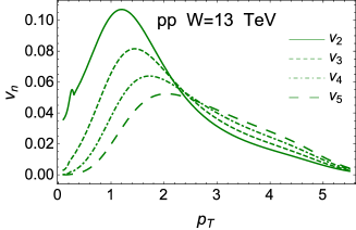
The calculation of vnsubscript𝑣𝑛v_{n} are shown in Fig. 9. One can see that we obtain large vnsubscript𝑣𝑛v_{n} for both odd and even n𝑛n. The value of v2subscript𝑣2v_{2} from Fig. 9-c is about 10% larger, than the experimental one from Ref.ATLASPP (see Fig. 7-b). However, our calculations lead to narrower distributions in pTsubscript𝑝𝑇p_{T} than the experimental one. The factorization VnΔ(pT1,pT2)=vn(pT1)vn(pT2)subscript𝑉𝑛Δsubscript𝑝𝑇1subscript𝑝𝑇2subscript𝑣𝑛subscript𝑝𝑇1subscript𝑣𝑛subscript𝑝𝑇2V_{n\Delta}\left(p_{T1},p_{T2}\right)\,=\,v_{n}\left(p_{T1}\right)\,v_{n}\left(p_{T2}\right) is strongly violated, as in the case of estimates of the first diagram.

Refer to caption Refer to caption Refer to caption
Fig. 9-a Fig. 9-b Fig. 9-c
Figure 9: vnsubscript𝑣𝑛v_{n} versus pTsubscript𝑝𝑇p_{T} for proton-proton scattering at W=13TeV𝑊13𝑇𝑒𝑉W=13\,TeV, using Eq. (91) and Eq. (12). Fig. 9-a shows vnsubscript𝑣𝑛v_{n} that stem from Eq. (12)-1. In Fig. 9-b the estimates from Eq. (12)-2 for pTRef=2GeVsubscriptsuperscript𝑝Ref𝑇2𝐺𝑒𝑉p^{\rm Ref}_{T}=2\,GeV are plotted. Fig. 9-b describes the same vnsubscript𝑣𝑛v_{n} as in Fig. 6-c but pTRefsubscriptsuperscript𝑝Ref𝑇p^{\rm Ref}_{T} is taken in the interval 0.5 to 5 GeV, as is measured in Ref.ATLASPP .

Fig. 7 illustrates the energy dependence of vnsubscript𝑣𝑛v_{n} for proton-proton scattering, showing v2subscript𝑣2v_{2} for two energies W=2.56TeV𝑊2.56𝑇𝑒𝑉W=2.56\,TeV and W=13TeV𝑊13𝑇𝑒𝑉W=13\,TeV. Note, that v2subscript𝑣2v_{2} does not depend on energy, in accord with the experimental data of Ref.ATLASPP .

Therefore, we can conclude that the first term in Eq. (15) leads to a value of vnsubscript𝑣𝑛v_{n}, which is large and of the order of the experimental one; the inclusion of diffraction in the region of small mass (sum over resonances in Eq. (15)) leads to a decrease of the interaction volume, but cannot reproduce the experimental pTsubscript𝑝𝑇p_{T} distributions of vnsubscript𝑣𝑛v_{n}, and BE correlations show the experimentally observed independence on energy.

II.2 Hadron-nucleus and nucleus nucleus interaction

For a nucleus we can simplify the calculation, considering cylindrical nuclei which have a form factor

SA(kT)=RAkTJ1(kTRA)subscript𝑆𝐴subscript𝑘𝑇subscript𝑅𝐴subscript𝑘𝑇subscript𝐽1subscript𝑘𝑇subscript𝑅𝐴S_{A}\left(k_{T}\right)\,=\,\frac{R_{A}}{k_{T}}\,J_{1}\left(k_{T}R_{A}\right) (21)

where J1subscript𝐽1J_{1} is the Bessel function. Taking Eq. (21) into account one can see that

CpA(R|𝒑T2𝒑T1|)subscript𝐶𝑝𝐴𝑅subscript𝒑𝑇2subscript𝒑𝑇1\displaystyle C_{pA}\left(R|\boldsymbol{p}_{T2}-\boldsymbol{p}_{T1}|\right)\,\, proportional-to\displaystyle\propto d2kTgIP,tr2((𝒌T𝒑T,12)2)SA2(kT2)/d2kTgIP,tr2((kT2)2)SA2(kT2)superscript𝑑2subscript𝑘𝑇subscriptsuperscript𝑔2𝐼𝑃trsuperscriptsubscript𝒌𝑇subscript𝒑𝑇122superscriptsubscript𝑆𝐴2subscriptsuperscript𝑘2𝑇superscript𝑑2subscript𝑘𝑇subscriptsuperscript𝑔2𝐼𝑃trsuperscriptsubscriptsuperscript𝑘2𝑇2superscriptsubscript𝑆𝐴2subscriptsuperscript𝑘2𝑇\displaystyle\,\,\int d^{2}k_{T}\,g^{2}_{{I\!\!P},{\rm tr}}\left(\left(\boldsymbol{k}_{T}-\boldsymbol{p}_{T,12}\right)^{2}\right)\,S_{A}^{2}\left(k^{2}_{T}\right)\Bigg{/}\int d^{2}k_{T}\,g^{2}_{{I\!\!P},{\rm tr}}\left(\left(k^{2}_{T}\right)^{2}\right)\,S_{A}^{2}\left(k^{2}_{T}\right) (22)
=\displaystyle= d2kTeB(kT2+pT,122)I0(2BkTpT,12)SA2(kT2)/d2kTeBkT2SA2(kT2)superscript𝑑2subscript𝑘𝑇superscript𝑒𝐵subscriptsuperscript𝑘2𝑇subscriptsuperscript𝑝2𝑇12subscript𝐼02𝐵subscript𝑘𝑇subscript𝑝𝑇12superscriptsubscript𝑆𝐴2subscriptsuperscript𝑘2𝑇superscript𝑑2subscript𝑘𝑇superscript𝑒𝐵subscriptsuperscript𝑘2𝑇superscriptsubscript𝑆𝐴2subscriptsuperscript𝑘2𝑇\displaystyle\int d^{2}k_{T}\,e^{-B\left(k^{2}_{T}+p^{2}_{T,12}\right)}\,I_{0}\left(2B\,k_{T}\,p_{T,12}\right)\,S_{A}^{2}\left(k^{2}_{T}\right)\Bigg{/}\int d^{2}k_{T}\,\,e^{-Bk^{2}_{T}}\,\,S_{A}^{2}\left(k^{2}_{T}\right)

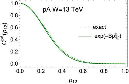
We expect that SA(kT)subscript𝑆𝐴subscript𝑘𝑇S_{A}\left(k_{T}\right) leads to small kT1/RAsimilar-tosubscript𝑘𝑇1subscript𝑅𝐴k_{T}\sim 1/R_{A}, since the radius of nucleus is large. In Fig. 10-a we compare Eq. (22) with exp(BpT,122)𝐵subscriptsuperscript𝑝2𝑇12\exp\left(-Bp^{2}_{T,12}\right) which follows from Eq. (22), replacing SA2(kT2)superscriptsubscript𝑆𝐴2subscriptsuperscript𝑘2𝑇S_{A}^{2}\left(k^{2}_{T}\right) by δ(kT)𝛿subscript𝑘𝑇\delta\left(k_{T}\right). The agreement is impressive.

Refer to caption Refer to caption
Fig. 10-a Fig. 10-b
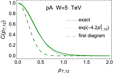
Figure 10: Fig. 10-a: comparison Eq. (22) with the same equation where SA2(kT2)superscriptsubscript𝑆𝐴2subscriptsuperscript𝑘2𝑇S_{A}^{2}\left(k^{2}_{T}\right) is replaced by δ(kT)𝛿subscript𝑘𝑇\delta\left(k_{T}\right). RA=6.5fmsubscript𝑅𝐴6.5𝑓𝑚R_{A}=6.5fm for gold. B=10GeV2𝐵10𝐺𝑒superscript𝑉2B=10\,GeV^{-2} for proton at W =13 TeV. Fig. 10-b: correlation function C(pT,12)𝐶subscript𝑝𝑇12C\left(p_{T,12}\right) for proton-lead scattering at W = 5 TeV in our model (see appendix C) as it is defined in Eq. (10), versus pT,12=|𝒑T1𝒑T2|subscript𝑝𝑇12subscript𝒑𝑇1subscript𝒑𝑇2p_{T,12}=|\boldsymbol{p}_{T1}-\boldsymbol{p}_{T2}|. Dashed line corresponds to exp(BpT,122)𝐵subscriptsuperscript𝑝2𝑇12\exp\left(-Bp^{2}_{T,12}\right) with B=4.2GeV2𝐵4.2𝐺𝑒superscript𝑉2B=4.2\,GeV^{-2}, while the dotted line shows the dependence that we used in section 2 to calculate the first diagram: exp(BpT,122)𝐵subscriptsuperscript𝑝2𝑇12\exp\left(-B\,p^{2}_{T,12}\right) with B=10GeV2𝐵10𝐺𝑒superscript𝑉2B=10\,GeV^{-2}

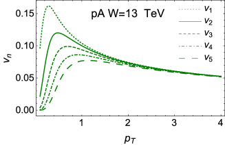
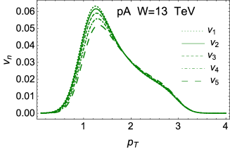
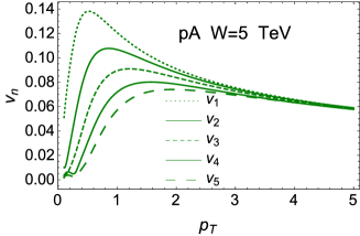
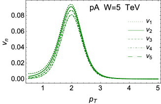
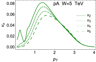
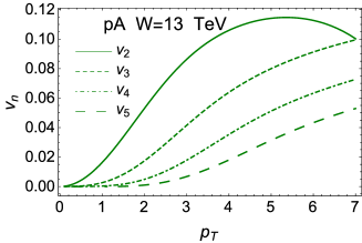
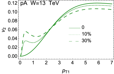
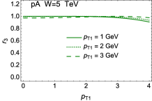
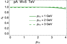
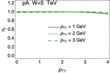
In Fig. 11 we plot the prediction for proton-gold scattering. One can see that the Bose-Einstein correlations generate large vnsubscript𝑣𝑛v_{n} for n 3𝑛3n\,\geq\,3. Actually, we have several mechanisms (see, for example, review of Ref.KOLUREV ) for vnsubscript𝑣𝑛v_{n} with even n𝑛n, therefore, it is instructive to note that the simple estimates in this section lead to large v2n1subscript𝑣2𝑛1v_{2n-1}, larger than has been measured ATLASPA . It should be stressed that using a more general approach which includes the diffractive production of small masses, as well as the shadowing corrections that lead to the shrinkage of diffractive peak, we obtain the predictions (see formulae in appendix C) which repeat the main features of our estimates in the simple model of Eq. (22). These calculations are plotted in Fig. 11-d - Fig. 11-f. In Fig. 10-b estimates for C(pT,12)𝐶subscript𝑝𝑇12C\left(p_{T,12}\right) in our model (see appendix C) are shown. One can see that C(pT,12)𝐶subscript𝑝𝑇12C\left(p_{T,12}\right) are different, and the model gives a smaller interaction volume. However, all qualitative features turn out to be the same: larger interaction volume than for proton-proton scattering, v2subscript𝑣2v_{2} is much smaller than the experimental value (see Fig. 12); v3subscript𝑣3v_{3}, v4subscript𝑣4v_{4} and even v5subscript𝑣5v_{5} are close to the experimental values; and the value of the typical pTsubscript𝑝𝑇p_{T} is about 1GeV1𝐺𝑒𝑉1\,GeV instead of pT=34GeVsubscript𝑝𝑇34𝐺𝑒𝑉p_{T}=3-4\,GeV in the experimental data.

Refer to caption Refer to caption Refer to caption
Fig. 11-a Fig. 11-b Fig. 11-c
Refer to caption Refer to caption Refer to caption
Fig. 11-d Fig. 11-e Fig. 11-f
Figure 11: vnsubscript𝑣𝑛v_{n} versus pTsubscript𝑝𝑇p_{T} for proton - gold (Fig. 11-a - Fig. 11-c) scattering at W=13TeV𝑊13𝑇𝑒𝑉W=13\,TeV and proton-lead scattering at W=5TeV𝑊5𝑇𝑒𝑉W=5\,TeV (Fig. 11-d - Fig. 11-c), using Eq. (19) and Eq. (12). Fig. 11-a and Fig. 11-d show vnsubscript𝑣𝑛v_{n} that stem from Eq. (12)-1. In Fig. 11-b and Fig. 11-e the estimates from Eq. (12)-2 for pTRef=2GeVsubscriptsuperscript𝑝Ref𝑇2𝐺𝑒𝑉p^{\rm Ref}_{T}=2\,GeV are plotted. Fig. 11-c and Fig. 11-f describe the same vnsubscript𝑣𝑛v_{n} as in Fig. 6-c but pTRefsubscriptsuperscript𝑝Ref𝑇p^{\rm Ref}_{T} is taken in the interval 13GeV13𝐺𝑒𝑉1-3\,GeV as it is measured in Ref.ATLASPA .
Refer to caption
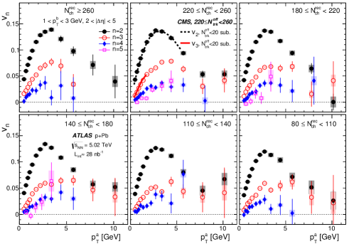
Figure 12: vnsubscript𝑣𝑛v_{n} versus pTsubscript𝑝𝑇p_{T} for proton - lead scattering at W=5TeV𝑊5𝑇𝑒𝑉W=5\,TeV measured by ATLAS collaborationATLASPP (Fig.9 from this paper)

For nucleus-nucleus interaction CAA(R|𝒑T2𝒑T1|)subscript𝐶𝐴𝐴𝑅subscript𝒑𝑇2subscript𝒑𝑇1C_{AA}\left(R|\boldsymbol{p}_{T2}-\boldsymbol{p}_{T1}|\right) takes the form

CAA(R|𝒑T2𝒑T1|)subscript𝐶𝐴𝐴𝑅subscript𝒑𝑇2subscript𝒑𝑇1\displaystyle C_{AA}\left(R|\boldsymbol{p}_{T2}-\boldsymbol{p}_{T1}|\right)\,\, proportional-to\displaystyle\propto d2kTSA2((𝒌T𝒑T,12)2)SA2(kT2)/d2kTSA2((kT2)2)SA2(kT2)superscript𝑑2subscript𝑘𝑇superscriptsubscript𝑆𝐴2superscriptsubscript𝒌𝑇subscript𝒑𝑇122superscriptsubscript𝑆𝐴2subscriptsuperscript𝑘2𝑇superscript𝑑2subscript𝑘𝑇subscriptsuperscript𝑆2𝐴superscriptsubscriptsuperscript𝑘2𝑇2superscriptsubscript𝑆𝐴2subscriptsuperscript𝑘2𝑇\displaystyle\,\,\int d^{2}k_{T}\,S_{A}^{2}\left(\left(\boldsymbol{k}_{T}-\boldsymbol{p}_{T,12}\right)^{2}\right)\,S_{A}^{2}\left(k^{2}_{T}\right)\Bigg{/}\int d^{2}k_{T}\,S^{2}_{A}\left(\left(k^{2}_{T}\right)^{2}\right)\,S_{A}^{2}\left(k^{2}_{T}\right) (23)

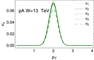
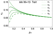
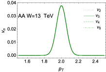
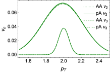
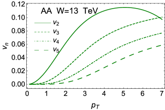
Fig. 13 shows vnsubscript𝑣𝑛v_{n} for gold-gold scattering. One can see three major differences: vnsubscript𝑣𝑛v_{n} values turns out to be smaller than for proton-nucleus scattering, especially when pT2=pTRefsubscript𝑝𝑇2subscriptsuperscript𝑝Ref𝑇p_{T2}=p^{\rm Ref}_{T} differs from pT1subscript𝑝𝑇1p_{T1}; the momentum distribution is much narrower than for pA𝑝𝐴pA scattering, and vnsubscript𝑣𝑛v_{n} are the same for all n𝑛n.

Refer to caption Refer to caption Refer to caption Refer to caption
Fig. 13-a Fig. 13-b Fig. 13-c Fig. 13-d
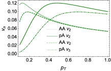
Figure 13: vnsubscript𝑣𝑛v_{n} versus pTsubscript𝑝𝑇p_{T} for gold - gold scattering at W=13TeV𝑊13𝑇𝑒𝑉W=13\,TeV, using Eq. (19) and Eq. (12). Fig. 13-a shows vnsubscript𝑣𝑛v_{n} that stem from Eq. (12)-1. In Fig. 13-b the estimates from Eq. (12)-2 for pTRef=2GeVsubscriptsuperscript𝑝Ref𝑇2𝐺𝑒𝑉p^{\rm Ref}_{T}=2\,GeV is plotted. Fig. 13c and Fig. 13-d describe the difference between proton-gold and gold-gold interactions.

Comparing Fig. 6, Fig. 11 and Fig. 13 we can conclude that the simplest estimates lead to sufficiently large vnsubscript𝑣𝑛v_{n} for both even and odd n𝑛n, which are similar to those obtained in proton-proton and proton-nucleus collisions, but they are considerably smaller for the nucleus-nucleus case. Comparing these predictions with the experimental data of Refs.CMSPP ; STARAA ; PHOBOSAA ; STARAA1 ; CMSPA ; CMSAA ; ALICEAA ; ALICEPA ; ATLASPP ; ATLASPA ; ATLASAA we see that the BE correlations should be taken into account in all three reactions, since they give sizable contributions.

III A brief review of our model

In this section we will give a brief review of our model which has been developed in our papers GLM2CH ; GLMNI . The advantage of the model is that it describes the experimental data on diffractive and elastic productionGLM2CH ; the inclusive production GLMINCL and large rapidity range (LRR) correlations GLMCOR .

As has been mentioned we need to build a model which incorporates at least two non-perturbative phenomena: the correct large b𝑏b behaviour of the amplitude and the hadron structure. These need to be incorporated so as to reproduce in the framework of one approach, the main features of the experimental data, such as the increase of the interaction radius with energy, a sufficiently large cross section of diffraction production, as well as energy and multiplicity dependence of inclusive cross sections and two particle correlations. On the other hand, we wish to include as much information as possible from a theoretical approach based on QCD.

III.1 Theoretical input and ‘dressed’ Pomeron Green function

At the moment, the effective theory for QCD at high energies exists in two different formulations: the CGC/saturation approach MV ; MUCD ; BK ; JIMWLK , and the BFKL Pomeron calculus BFKL ; GLR ; MUQI ; MUPA ; BART ; BRN ; KOLE ; LELU ; LMP ; AKLL ; AKLL1 ; LEPP . In building our model we rely on the BFKL Pomeron calculus, since the relation to diffractive physics is more evident in this approach. However, we are aware that the CGC/saturation approach gives a more general patternAKLL ; AKLL1 . In Ref.AKLL1 it was proven that these two approaches are equivalent for

Y2ΔBFKLln(1ΔBFKL2)𝑌2subscriptΔBFKL1subscriptsuperscriptΔ2BFKLY\,\leq\,\frac{2}{\Delta_{\mbox{\tiny BFKL}}}\,\ln\left(\frac{1}{\Delta^{2}_{\mbox{\tiny BFKL}}}\right) (24)

where ΔBFKLsubscriptΔBFKL\Delta_{\mbox{\tiny BFKL}} denotes the intercept of the BFKL Pomeron. As we will see, in our model ΔBFKL 0.20.25subscriptΔBFKL0.20.25\Delta_{\mbox{\tiny BFKL}}\,\approx\,0.2-0.25 leading to Ymax=2030subscript𝑌𝑚𝑎𝑥2030Y_{max}=20-30, which covers all accessible energies. In addition in Ref.AKLL1 it is shown that for such Y𝑌Y, we can safely use the Mueller-Patel-Salam-Iancu (MPSI) approachMPSI , which allows us to calculate the contribution to the resulting BFKL Pomeron Green function ( see Fig. 14-a):

GIPdressed(Y,r,R;b)=subscriptsuperscript𝐺dressed𝐼𝑃𝑌𝑟𝑅𝑏absent\displaystyle G^{\mbox{\tiny dressed}}_{I\!\!P}\left(Y,r,R;b\right)\,\,= (25)
i=1d2rid2bid2rid2biN(YY,r,{ri,bbi})Adipole-dipoleBA(ri,ri,𝒃i𝒃i)N(Y,R,{ri,bi})subscriptproduct𝑖1superscript𝑑2subscript𝑟𝑖superscript𝑑2subscript𝑏𝑖superscript𝑑2subscriptsuperscript𝑟𝑖superscript𝑑2subscriptsuperscript𝑏𝑖𝑁𝑌superscript𝑌𝑟subscript𝑟𝑖𝑏subscript𝑏𝑖subscriptsuperscript𝐴BAdipole-dipolesubscript𝑟𝑖subscriptsuperscript𝑟𝑖subscript𝒃𝑖subscriptsuperscript𝒃bold-′𝑖𝑁superscript𝑌𝑅subscriptsuperscript𝑟𝑖subscriptsuperscript𝑏𝑖\displaystyle\,\,\int\prod_{i=1}d^{2}r_{i}\,d^{2}b_{i}\,d^{2}r^{\prime}_{i}\,d^{2}b^{\prime}_{i}\,N\left(Y-Y^{\prime},r,\{r_{i},b-b_{i}\}\right)\,A^{\rm BA}_{\mbox{\tiny dipole-dipole}}\left(r_{i},r^{\prime}_{i},\boldsymbol{b}_{i}-\boldsymbol{b^{\prime}}_{i}\right)N\left(Y^{\prime},R,\{r^{\prime}_{i},b^{\prime}_{i}\}\right)

where Adipole-dipoleBAsubscriptsuperscript𝐴𝐵𝐴dipole-dipoleA^{BA}_{\mbox{\tiny dipole-dipole}} is the dipole-dipole scattering amplitude in the Born approximation of perturbative QCD, and is shown in Fig. 14-a by the red circles.

Refer to caption
Figure 14: Fig. 14-a shows the set of the diagrams in the BFKL Pomeron calculus that produce the resulting (dressed) Green function of the Pomeron in the framework of high energy QCD. The red blobs denote the amplitude of dipole-dipole interaction at low energy. In Fig. 14-b the net diagrams, which include the interaction of the BFKL Pomerons with colliding hadrons, are shown. The sum of the diagrams after integration over positions of G3IPsubscript𝐺3𝐼𝑃G_{3{I\!\!P}} in rapidity, reduces to Fig. 14-c.

We need to find the amplitude for the production of dipoles of size risubscript𝑟𝑖r_{i} at impact parameters bisubscript𝑏𝑖b_{i}. This amplitude can be written as (see Fig. 14-c)

N(YY,r,{ri,bi})=𝑁𝑌superscript𝑌𝑟subscript𝑟𝑖subscript𝑏𝑖absent\displaystyle N\left(Y-Y^{\prime},r,\{r_{i},b_{i}\}\right)\,\,= (26)
n=1( 1)n+1C~n(ϕ0,r)i=1nGIP(YY;r,ri,bi)=n=1( 1)n+1C~n(ϕ0,r)i=1nGIP(zzi).subscriptsuperscript𝑛1superscript1𝑛1subscript~𝐶𝑛subscriptitalic-ϕ0𝑟subscriptsuperscriptproduct𝑛𝑖1subscript𝐺𝐼𝑃𝑌superscript𝑌𝑟subscript𝑟𝑖subscript𝑏𝑖subscriptsuperscript𝑛1superscript1𝑛1subscript~𝐶𝑛subscriptitalic-ϕ0𝑟subscriptsuperscriptproduct𝑛𝑖1subscript𝐺𝐼𝑃𝑧subscript𝑧𝑖\displaystyle\,\,\sum^{\infty}_{n=1}\,\left(-\,1\right)^{n+1}\widetilde{C}_{n}\left(\phi_{0},r\right)\prod^{n}_{i=1}G_{I\!\!P}\left(Y-Y^{\prime};r,r_{i},b_{i}\right)\,\,=\,\,\sum^{\infty}_{n=1}\,\left(-\,1\right)^{n+1}\widetilde{C}_{n}\left(\phi_{0},r\right)\prod^{n}_{i=1}G_{I\!\!P}\left(z-z_{i}\right).

C~n(ϕ0,r)subscript~𝐶𝑛subscriptitalic-ϕ0𝑟\widetilde{C}_{n}\left(\phi_{0},r\right) is shown as the multi-Pomeron amplitudes ( pink ovals) in Fig. 14-c.

The solution to the non-linear equation is of the following general form

N(GIP(ϕ0,z))=n=1( 1)n+1Cn(ϕ0)GIPn(ϕ0,z).𝑁subscript𝐺𝐼𝑃subscriptitalic-ϕ0𝑧subscriptsuperscript𝑛1superscript1𝑛1subscript𝐶𝑛subscriptitalic-ϕ0superscriptsubscript𝐺𝐼𝑃𝑛subscriptitalic-ϕ0𝑧N\left(G_{I\!\!P}\left(\phi_{0},z\right)\right)\,\,=\,\,\sum^{\infty}_{n=1}\,\left(-\,1\right)^{n+1}C_{n}\left(\phi_{0}\right)G_{I\!\!P}^{n}\left(\phi_{0},z\right). (27)

Comparing Eq. (26) with Eq. (27) we see

C~n(ϕ0,r)=Cn(ϕ0).subscript~𝐶𝑛subscriptitalic-ϕ0𝑟subscript𝐶𝑛subscriptitalic-ϕ0\widetilde{C}_{n}\left(\phi_{0},r\right)\,\,\,=\,\,\,C_{n}\left(\phi_{0}\right). (28)

Coefficients Cnsubscript𝐶𝑛C_{n} can be found from the solution to the Balitsky-Kovchegov equation BK in the saturation region (see Ref.LEPP ).

NBK(GIP(ϕ0,z))=a(1exp(GIP(ϕ0,z)))+(1a)GIP(ϕ0,z)1+GIP(ϕ0,z),superscript𝑁BKsubscript𝐺𝐼𝑃subscriptitalic-ϕ0𝑧𝑎1subscript𝐺𝐼𝑃subscriptitalic-ϕ0𝑧1𝑎subscript𝐺𝐼𝑃subscriptitalic-ϕ0𝑧1subscript𝐺𝐼𝑃subscriptitalic-ϕ0𝑧N^{\rm BK}\left(G_{I\!\!P}\left(\phi_{0},z\right)\right)\,\,=\,\,a\,\left(1-\exp\left(-G_{I\!\!P}\left(\phi_{0},z\right)\right)\right)\,\,+\,\,\left(1-a\right)\frac{G_{I\!\!P}\left(\phi_{0},z\right)}{1\,+\,G_{I\!\!P}\left(\phi_{0},z\right)}, (29)

with a𝑎a = 0.65. Eq. (29) is a convenient parameterization of the numerical solution within accuracy better than 5%. Having Cnsubscript𝐶𝑛C_{n} we can calculate the Green function of the dressed BFKL Pomeron using Eq. (25) and the property of the BFKL Pomeron exchange:

αS24πGIP(Y0,r,R;b)=superscriptsubscript𝛼𝑆24𝜋subscript𝐺𝐼𝑃𝑌0𝑟𝑅𝑏absent\displaystyle\frac{\alpha_{S}^{2}}{4\pi}\,\,G_{I\!\!P}\left(Y-0,r,R;b\right)\,=\, (30)
d2rd2bd2r′′d2b′′GIP(YY,r,r,𝒃𝒃)GIP(Yr′′,R,𝒃′′)Adipole-dipoleBA(r,r′′,𝒃′′𝒃)superscript𝑑2superscript𝑟superscript𝑑2superscript𝑏superscript𝑑2superscript𝑟′′superscript𝑑2superscript𝑏′′subscript𝐺𝐼𝑃𝑌superscript𝑌𝑟superscript𝑟𝒃superscript𝒃subscript𝐺𝐼𝑃superscript𝑌superscript𝑟′′𝑅superscript𝒃′′subscriptsuperscript𝐴BAdipole-dipolesuperscript𝑟superscript𝑟′′superscript𝒃bold-′′superscript𝒃bold-′\displaystyle\int d^{2}r^{\prime}d^{2}b^{\prime}\,d^{2}r^{\prime\prime}\,d^{2}b^{\prime\prime}\,G_{I\!\!P}\left(Y-Y^{\prime},r,r^{\prime},\boldsymbol{b}-\boldsymbol{b}^{\,{}^{\prime}}\right)\,\,\,G_{I\!\!P}\left(Y^{\prime}r^{\prime\prime},R,\boldsymbol{b}^{\,{}^{\prime\prime}}\right)\,\,A^{\rm BA}_{\mbox{\tiny dipole-dipole}}\left(r^{\prime},r^{\prime\prime},\boldsymbol{b^{\prime\prime}}-\boldsymbol{b^{\prime}}\right)

Carrying out the integrations in Eq. (25), we obtain the Green function of the dressed Pomeron in the following form:

Gdressed(T)superscript𝐺dressed𝑇\displaystyle G^{\mbox{\tiny dressed}}\left(T\right)\,\, =\displaystyle= a2(1exp(T))+2a(1a)T1+T+(1a)2G(T)superscript𝑎21𝑇2𝑎1𝑎𝑇1𝑇superscript1𝑎2𝐺𝑇\displaystyle\,\,a^{2}(1-\exp\left(-T\right))+2a(1-a)\frac{T}{1+T}+(1-a)^{2}G\left(T\right)
with G(T)=11Texp(1T)Γ(0,1T)𝐺𝑇11𝑇1𝑇Γ01𝑇\displaystyle~{}~{}G\left(T\right)=1-\frac{1}{T}\exp\left(\frac{1}{T}\right)\Gamma\left(0,\frac{1}{T}\right) (31)

where Γ(s,z)Γ𝑠𝑧\Gamma\left(s,z\right) is the upper incomplete gamma function (see Ref.RY formula 8.35) and T𝑇T is the BFKL Pomeron in the vicinity of the saturation scale

T(r,s,b)=ϕ0(r2Qs2(Y,b))γ¯𝑇subscript𝑟bottom𝑠𝑏subscriptitalic-ϕ0superscriptsubscriptsuperscript𝑟2bottomsubscriptsuperscript𝑄2𝑠𝑌𝑏¯𝛾T\left(r_{\bot},s,b\right)\,\,=\,\,\phi_{0}\left(r^{2}_{\bot}Q^{2}_{s}\left(Y,b\right)\right)^{\bar{\gamma}} (32)

III.2 Phenomenological assumptions and phenomenological parameters

The first phenomenological idea, is to fix the large impact parameter behaviour by assuming that the saturation momentum depends on b𝑏b in the following way:

Qs2(b,Y)=Q0s2(b,Y0)eλ(YY0)subscriptsuperscript𝑄2𝑠𝑏𝑌subscriptsuperscript𝑄20𝑠𝑏subscript𝑌0superscript𝑒𝜆𝑌subscript𝑌0Q^{2}_{s}\left(b,Y\right)\,\,=\,\,Q^{2}_{0s}\left(b,Y_{0}\right)\,e^{\lambda\,(Y-Y_{0})} (33)

with

Q0s2(b,Y0)=(m2)11/γ¯(S(b,m))1/γ¯S(b,m)=m22πembandγ¯= 0.63formulae-sequencesubscriptsuperscript𝑄20𝑠𝑏subscript𝑌0superscriptsuperscript𝑚211¯𝛾superscript𝑆𝑏𝑚1¯𝛾𝑆𝑏𝑚superscript𝑚22𝜋superscript𝑒𝑚𝑏and¯𝛾0.63Q^{2}_{0s}\left(b,Y_{0}\right)\,\,=\,\,\left(m^{2}\right)^{1-1/\bar{\gamma}}\,\left(S\left(b,m\right)\right)^{1/\bar{\gamma}}~{}~{}~{}~{}~{}~{}~{}S\left(b,m\right)\,\,=\,\,\frac{m^{2}}{2\pi}e^{-mb}~{}~{}~{}\mbox{and}~{}~{}\bar{\gamma}\,=\,0.63 (34)

We have introduced a new phenomenological parameter m𝑚m to describe the large b𝑏b behaviour. The Y𝑌Y dependence as well as r2superscript𝑟2r^{2} dependence, can be found from CGC/saturation approach KOLEB , since ϕ0subscriptitalic-ϕ0\phi_{0} and λ𝜆\lambda can be calculated in the leading order of perturbative QCD. However, since the higher order corrections turn out to be large HOCOR we treat them as parameters to be fitted. m𝑚m is non-perturbative parameter which determines the typical sizes of dipoles inside hadrons. As one can see from Table 1 from the fit m𝑚m = 5.25 GeV, supporting our main assumption that we can apply the BFKL Pomeron calculus, based on perturbative QCD, to the soft interaction since mμsoftmuch-greater-than𝑚subscript𝜇𝑠𝑜𝑓𝑡m\,\gg\,\mu_{soft} where μsoftsubscript𝜇𝑠𝑜𝑓𝑡\mu_{soft} is the scale of soft interaction, which is of the order of the mass of pion or ΛQCDsubscriptΛQCD\Lambda_{\rm QCD}.

Unfortunately, since the confinement problem is far from being solved, we have to assume a phenomenological approach for the structure of the colliding hadrons. We use a two channel model, which allows us to calculate the diffractive production in the region of small masses. In this model, we replace the rich structure of the diffractively produced states, by a single state with the wave function ψDsubscript𝜓𝐷\psi_{D}, a la Good-Walker GW . The observed physical hadronic and diffractive states are written in the form

ψh=αΨ1+βΨ2;ψD=βΨ1+αΨ2;whereα2+β2= 1;formulae-sequencesubscript𝜓𝛼subscriptΨ1𝛽subscriptΨ2formulae-sequencesubscript𝜓𝐷𝛽subscriptΨ1𝛼subscriptΨ2wheresuperscript𝛼2superscript𝛽21\psi_{h}\,=\,\alpha\,\Psi_{1}+\beta\,\Psi_{2}\,;\,\,\,\,\,\,\,\,\,\,\psi_{D}\,=\,-\beta\,\Psi_{1}+\alpha\,\Psi_{2};~{}~{}~{}~{}~{}~{}~{}~{}~{}\mbox{where}~{}~{}~{}~{}~{}~{}~{}\alpha^{2}+\beta^{2}\,=\,1; (35)

Functions ψ1subscript𝜓1\psi_{1} and ψ2subscript𝜓2\psi_{2} form a complete set of orthogonal functions {ψi}subscript𝜓𝑖\{\psi_{i}\} which diagonalize the interaction matrix T𝑇T

Ai,kik=<ψiψk|𝐓|ψiψk>=Ai,kδi,iδk,k.subscriptsuperscript𝐴superscript𝑖superscript𝑘𝑖𝑘quantum-operator-productsubscript𝜓𝑖subscript𝜓𝑘𝐓subscript𝜓superscript𝑖subscript𝜓superscript𝑘subscript𝐴𝑖𝑘subscript𝛿𝑖superscript𝑖subscript𝛿𝑘superscript𝑘A^{i^{\prime}k^{\prime}}_{i,k}=<\psi_{i}\,\psi_{k}|\mathbf{T}|\psi_{i^{\prime}}\,\psi_{k^{\prime}}>=A_{i,k}\,\delta_{i,i^{\prime}}\,\delta_{k,k^{\prime}}. (36)

The unitarity constraints take the form

2ImAi,k(s,b)=|Ai,k(s,b)|2+Gi,kin(s,b),2Imsubscript𝐴𝑖𝑘𝑠𝑏superscriptsubscript𝐴𝑖𝑘𝑠𝑏2subscriptsuperscript𝐺𝑖𝑛𝑖𝑘𝑠𝑏2\,\mbox{Im}\,A_{i,k}\left(s,b\right)=|A_{i,k}\left(s,b\right)|^{2}+G^{in}_{i,k}(s,b), (37)

where Gi,kinsubscriptsuperscript𝐺𝑖𝑛𝑖𝑘G^{in}_{i,k} denotes the contribution of all non diffractive inelastic processes, i.e. it is the summed probability for these final states to be produced in the scattering of a state i𝑖i off a state k𝑘k. In Eq. (37) s=W𝑠𝑊\sqrt{s}=W denotes the energy of the colliding hadrons, and b𝑏b the impact parameter. A simple solution to Eq. (37) at high energies, has the eikonal form with an arbitrary opacity ΩiksubscriptΩ𝑖𝑘\Omega_{ik}, where the real part of the amplitude is much smaller than the imaginary part.

Ai,k(s,b)=i(1exp(Ωi,k(s,b))),subscript𝐴𝑖𝑘𝑠𝑏𝑖1subscriptΩ𝑖𝑘𝑠𝑏A_{i,k}(s,b)=i\left(1-\exp\left(-\Omega_{i,k}(s,b)\right)\right), (38)
Gi,kin(s,b)=1exp(2Ωi,k(s,b)).subscriptsuperscript𝐺𝑖𝑛𝑖𝑘𝑠𝑏12subscriptΩ𝑖𝑘𝑠𝑏G^{in}_{i,k}(s,b)=1-\exp\left(-2\,\Omega_{i,k}(s,b)\right). (39)

Eq. (39) implies that Pi,kS=exp(2Ωi,k(s,b))subscriptsuperscript𝑃𝑆𝑖𝑘2subscriptΩ𝑖𝑘𝑠𝑏P^{S}_{i,k}=\exp\left(-2\,\Omega_{i,k}(s,b)\right), is the probability that the initial projectiles (i,k)𝑖𝑘(i,k) reach the final state interaction unchanged, regardless of the initial state re-scatterings.

III.3 Small parameters from the fit and the scattering amplitude

The first approach is to use the eikonal approximation for ΩΩ\Omega in which

Ωi,k(r,YY0,b)=d2bd2b′′gi(𝒃)Gdressed(T(r,YY0,𝒃′′))gk(𝒃𝒃𝒃′′)subscriptΩ𝑖𝑘subscript𝑟bottom𝑌subscript𝑌0𝑏superscript𝑑2superscript𝑏superscript𝑑2superscript𝑏′′subscript𝑔𝑖superscript𝒃superscript𝐺dressed𝑇subscript𝑟bottom𝑌subscript𝑌0superscript𝒃′′subscript𝑔𝑘𝒃superscript𝒃superscript𝒃′′\Omega_{i,k}(r_{\bot},Y-Y_{0},b)\,\,=\,\int d^{2}b^{\prime}\,d^{2}b^{\prime\prime}\,g_{i}\left(\boldsymbol{b}^{\prime}\right)\,G^{\mbox{\tiny dressed}}\left(T\left(r_{\bot},Y-Y_{0},\boldsymbol{b}^{\prime\prime}\right)\right)\,g_{k}\left(\boldsymbol{b}-\boldsymbol{b}^{\prime}\ -\boldsymbol{b}^{\prime\prime}\right) (40)

We propose a more general approach, which takes into account new small parameters, that come from the fit to the experimental data (see Table 1 and Fig. 14 for notations):

G3IP/gi(b=0)  1;mm1andm2formulae-sequencemuch-less-thansubscript𝐺3𝐼𝑃subscript𝑔𝑖𝑏01much-greater-than𝑚subscript𝑚1andsubscript𝑚2G_{3{I\!\!P}}\Big{/}g_{i}(b=0)\,\ll\,\,1;~{}~{}~{}~{}~{}~{}~{}~{}m\,\gg\,m_{1}~{}\mbox{and}~{}m_{2} (41)

The second equation in Eq. (41) leads to the fact that b′′superscript𝑏′′b^{\prime\prime} in Eq. (40) is much smaller than b𝑏b and bsuperscript𝑏b^{\prime}, therefore, Eq. (40) can be re-written in a simpler form

Ωi,k(r,YY0,b)subscriptΩ𝑖𝑘subscript𝑟bottom𝑌subscript𝑌0𝑏\displaystyle\Omega_{i,k}(r_{\bot},Y-Y_{0},b)\,\, =\displaystyle= (d2b′′Gdressed(T(r,YY0,𝒃′′)))d2bgi(𝒃)gk(𝒃𝒃)superscript𝑑2superscript𝑏′′superscript𝐺dressed𝑇subscript𝑟bottom𝑌subscript𝑌0superscript𝒃′′superscript𝑑2superscript𝑏subscript𝑔𝑖superscript𝒃subscript𝑔𝑘𝒃superscript𝒃\displaystyle\,\Bigg{(}\int d^{2}b^{\prime\prime}\,G^{\mbox{\tiny dressed}}\left(T\left(r_{\bot},Y-Y_{0},\boldsymbol{b}^{\prime\prime}\right)\right)\Bigg{)}\,\int d^{2}b^{\prime}g_{i}\left(\boldsymbol{b}^{\prime}\right)\,g_{k}\left(\boldsymbol{b}-\boldsymbol{b}^{\prime}\right)\, (42)
=\displaystyle= G~dressed(r,YY0)d2bgi(𝒃)gk(𝒃𝒃)superscript~𝐺dressedsubscript𝑟bottom𝑌subscript𝑌0superscript𝑑2superscript𝑏subscript𝑔𝑖superscript𝒃subscript𝑔𝑘𝒃superscript𝒃\displaystyle\,\tilde{G}^{\mbox{\tiny dressed}}\left(r_{\bot},Y-Y_{0}\right)\,\,\int d^{2}b^{\prime}g_{i}\left(\boldsymbol{b}^{\prime}\right)\,g_{k}\left(\boldsymbol{b}-\boldsymbol{b}^{\prime}\right)

Using the first small parameter of Eq. (41), we can see that the main contribution stems from the net diagrams shown in Fig. 14-b. The sum of these diagramsGLM2CH leads to the following expression for Ωi,k(s,b)subscriptΩ𝑖𝑘𝑠𝑏\Omega_{i,k}(s,b)

Ω(r,YY0;b)Ωsubscript𝑟bottom𝑌subscript𝑌0𝑏\displaystyle\Omega\left(r_{\bot},Y-Y_{0};b\right)~{}~{} =\displaystyle= d2bgi(𝒃)gk(𝒃𝒃)G~dressed(r,YY0)1+G3IPG~dressed(r,YY0)[gi(𝒃)+gk(𝒃𝒃)];superscript𝑑2superscript𝑏subscript𝑔𝑖superscript𝒃subscript𝑔𝑘𝒃superscript𝒃superscript~𝐺dressedsubscript𝑟bottom𝑌subscript𝑌01subscript𝐺3𝐼𝑃superscript~𝐺dressedsubscript𝑟bottom𝑌subscript𝑌0delimited-[]subscript𝑔𝑖superscript𝒃subscript𝑔𝑘𝒃superscript𝒃\displaystyle~{}~{}\int d^{2}b^{\prime}\,\,\,\,\frac{g_{i}\left(\boldsymbol{b}^{\prime}\right)\,g_{k}\left(\boldsymbol{b}-\boldsymbol{b}^{\prime}\right)\,\tilde{G}^{\mbox{\tiny dressed}}\left(r_{\bot},Y-Y_{0}\right)}{1\,+\,G_{3{I\!\!P}}\,\tilde{G}^{\mbox{\tiny dressed}}\left(r_{\bot},Y-Y_{0}\right)\left[g_{i}\left(\boldsymbol{b}^{\prime}\right)+g_{k}\left(\boldsymbol{b}-\boldsymbol{b}^{\prime}\right)\right]}; (43)
gi(b)subscript𝑔𝑖𝑏\displaystyle g_{i}\left(b\right)~{}~{} =\displaystyle= giSp(b;mi);subscript𝑔𝑖subscript𝑆𝑝𝑏subscript𝑚𝑖\displaystyle~{}~{}g_{i}\,S_{p}\left(b;m_{i}\right); (44)

where

Sp(b,mi)=14πmi3bK1(mib)subscript𝑆𝑝𝑏subscript𝑚𝑖14𝜋subscriptsuperscript𝑚3𝑖𝑏subscript𝐾1subscript𝑚𝑖𝑏S_{p}\left(b,m_{i}\right)\,=\,\frac{1}{4\pi}m^{3}_{i}\,b\,K_{1}\left(m_{i}b\right) (45)
G~dressed(r,YY0)=d2bGdressed(T(r,YY0,b))superscript~𝐺dressedsubscript𝑟bottom𝑌subscript𝑌0superscript𝑑2𝑏superscript𝐺dressed𝑇subscript𝑟bottom𝑌subscript𝑌0𝑏\tilde{G}^{\mbox{\tiny dressed}}\left(r_{\bot},Y-Y_{0}\right)\,\,=\,\,\int d^{2}b\,\,G^{\mbox{\tiny dressed}}\left(T\left(r_{\bot},Y-Y_{0},b\right)\right) (46)

where T(r,YY0,b)𝑇subscript𝑟bottom𝑌subscript𝑌0𝑏T\left(r_{\bot},Y-Y_{0},b\right) is given by Eq. (32).

Note that G~dressed(YY0)superscript~𝐺dressed𝑌subscript𝑌0\tilde{G}^{\mbox{\tiny dressed}}\left(Y-Y_{0}\right) does not depend on b𝑏b. In all previous formulae, the value of the triple BFKL Pomeron vertex is known: G3IP=1.29GeV1subscript𝐺3𝐼𝑃1.29𝐺𝑒superscript𝑉1G_{3{I\!\!P}}=1.29\,GeV^{-1}.

model λ𝜆\lambda ϕ0subscriptitalic-ϕ0\phi_{0} (GeV2𝐺𝑒superscript𝑉2GeV^{-2}) g1subscript𝑔1g_{1} (GeV1𝐺𝑒superscript𝑉1GeV^{-1}) g2subscript𝑔2g_{2} (GeV1𝐺𝑒superscript𝑉1GeV^{-1}) m(GeV)𝑚𝐺𝑒𝑉m(GeV) m1(GeV)subscript𝑚1𝐺𝑒𝑉m_{1}(GeV) m2(GeV)subscript𝑚2𝐺𝑒𝑉m_{2}(GeV) β𝛽\beta aIPIPsubscript𝑎𝐼𝑃𝐼𝑃a_{{I\!\!P}{I\!\!P}}
2 channel 0.38 0.0019 110.2 11.2 5.25 0.92 1.9 0.58 0.21
Table 1: Fitted parameters of the model. The values are taken from Ref.GLM2CH .

To simplify further discussion, we introduce the notation

NBK(GIPi(r,Y,b))=a(1exp(GIPi(r,Y,b)))+(1a)GIPi(r,Y,b)1+GIPi(r,Y,b),superscript𝑁𝐵𝐾subscriptsuperscript𝐺𝑖𝐼𝑃subscript𝑟bottom𝑌𝑏𝑎1subscriptsuperscript𝐺𝑖𝐼𝑃subscript𝑟bottom𝑌𝑏1𝑎subscriptsuperscript𝐺𝑖𝐼𝑃subscript𝑟bottom𝑌𝑏1subscriptsuperscript𝐺𝑖𝐼𝑃subscript𝑟bottom𝑌𝑏N^{BK}\left(G^{i}_{I\!\!P}\left(r_{\bot},Y,b\right)\right)\,\,=\,\,a\,\left(1-\exp\left(-G^{i}_{I\!\!P}\left(r_{\bot},Y,b\right)\right)\right)\,\,+\,\,\left(1-a\right)\frac{G^{i}_{I\!\!P}\left(r_{\bot},Y,b\right)}{1\,+\,G^{i}_{I\!\!P}\left(r_{\bot},Y,b\right)}, (47)

with a=0.65𝑎0.65a=0.65 . Eq. (47) is an analytical approximation to the numerical solution for the BK equationLEPP . GIPi(r,Y;b)=gi(b)G~dressed(r,YY0)subscriptsuperscript𝐺𝑖𝐼𝑃subscript𝑟bottom𝑌𝑏subscript𝑔𝑖𝑏superscript~𝐺dressedsubscript𝑟bottom𝑌subscript𝑌0G^{i}_{I\!\!P}\left(r_{\bot},Y;b\right)\,=\,\,g_{i}\left(b\right)\,\tilde{G}^{\mbox{\tiny dressed}}\left(r_{\bot},Y-Y_{0}\right). We recall that the BK equation sums the ‘fan’ diagrams.

For the elastic amplitude we have

ael(b)=(α4A1,1+ 2α2β2A1,2+β4A2,2).subscript𝑎𝑒𝑙𝑏superscript𝛼4subscript𝐴112superscript𝛼2superscript𝛽2subscript𝐴12superscript𝛽4subscript𝐴22a_{el}(b)\,=\,\left(\alpha^{4}A_{1,1}\,+\,2\alpha^{2}\,\beta^{2}\,A_{1,2}\,+\,\beta^{4}A_{2,2}\right). (48)

We will discuss the inclusive production as well as LRR correlations in appendix B.

IV Azimuthal angle correlation and the structure of the ‘dressed’ Pomeron

As has been discussed, our model includes three dimensional scales: m𝑚m,m1subscript𝑚1m_{1} and m2subscript𝑚2m_{2}. m1subscript𝑚1m_{1} and m2subscript𝑚2m_{2} describe two typical sizes in the proton wave function, which could be associated with the distance between constituent quarks (size of proton) Rp1/m1similar-tosubscript𝑅𝑝1subscript𝑚1R_{p}\sim 1/m_{1} and the size of the constituent quark Rq1/m2similar-tosubscript𝑅𝑞1subscript𝑚2R_{q}\sim 1/m_{2} in the framework of the constituent quark model CQM . The third scale: m𝑚m, characterizes the impact parameter behaviour of the saturation scale, and is intimately related to the structure of the dressed Pomeron in our model. In section 2 we discussed how two scales in the proton wave function arise in the BE correlations. Here, we would like to show that the third scale leads to the BE correlations which can explain the values of vnsubscript𝑣𝑛v_{n} observed experimentally.

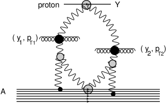
As we have discussed in section 3-A , the dressed Pomeron is the sum of enhanced diagrams (see Fig. 14-a) which is given by Eq. (III.1). Therefore, the exchange of the dressed Pomeron generates the production of an infinite number of the parton showers and, in particular, two parton showers which generate the BE correlations as is shown in Fig. 15. Integration over rapidities of triple Pomeron verticesLMP reduces the diagrams of Fig. 15-a and Fig. 15-b to the diagrams of Fig. 15-c and Fig. 15-d. We can calculate the probability to find two parton showers (P2subscript𝑃2P_{2}) inside of the dressed Pomeron expanding Eq. (III.1):

P2=(22a+a2/3)= 0.91fora=0.65formulae-sequencesubscript𝑃222𝑎superscript𝑎230.91for𝑎0.65P_{2}\,=\,(2-2a+a^{2}/3)\,=\,0.91\,\,\,\,\,\,\mbox{for}\,\,\,\,\,\,a=0.65 (49)

and the contribution of two parton showers production to the double inclusive cross section for the diagrams of Fig. 15-a, is equal to

d2σdy1dy2d2pT1d2pT2=aIPIP2P22d2kTT(kT,Yy1)T(kT,Yy2)T(kT,y1)T(kT,y2)superscript𝑑2𝜎𝑑subscript𝑦1𝑑subscript𝑦2superscript𝑑2subscript𝑝𝑇1superscript𝑑2subscript𝑝𝑇2subscriptsuperscript𝑎2𝐼𝑃𝐼𝑃subscriptsuperscript𝑃22superscript𝑑2subscript𝑘𝑇𝑇subscript𝑘𝑇𝑌subscript𝑦1𝑇subscript𝑘𝑇𝑌subscript𝑦2𝑇subscript𝑘𝑇subscript𝑦1𝑇subscript𝑘𝑇subscript𝑦2\frac{d^{2}\sigma}{dy_{1}\,dy_{2}d^{2}p_{T1}d^{2}p_{T2}}\,\,=\,\,a^{2}_{{I\!\!P}{I\!\!P}}\,P^{2}_{2}\,\int d^{2}k_{T}\,\,T\left(k_{T},Y-y_{1}\right)\,T\left(k_{T},Y-y_{2}\right)\,T\left(k_{T},y_{1}\right)\,T\left(k_{T},\ y_{2}\right) (50)

where aIPIPsubscript𝑎𝐼𝑃𝐼𝑃a_{{I\!\!P}{I\!\!P}} denotes the Mueller vertex of gluon emission (see Fig. 15). In our estimates for the calculation of vnsubscript𝑣𝑛v_{n}, we do not need to know the probability P2subscript𝑃2P_{2}, as well as the vertex aIPIPsubscript𝑎𝐼𝑃𝐼𝑃a_{{I\!\!P}{I\!\!P}}, assuming that aIPIPsubscript𝑎𝐼𝑃𝐼𝑃a_{{I\!\!P}{I\!\!P}} is the same in Fig. 15-a and in Fig. 15-b. In Eq. (50) all rapidities are in the laboratory frame.

T(kT,y)𝑇subscript𝑘𝑇𝑦T\left(k_{T},y\right) is the Fourier image of T(b,y)𝑇𝑏𝑦T\left(b,y\right) defined in Eq. (32)-Eq. (34) and it takes the form

T(kT,y)=ϕ01(1+kT2m2)3/2eλγ¯(YY0)𝑇subscript𝑘𝑇𝑦subscriptitalic-ϕ01superscript1subscriptsuperscript𝑘2𝑇superscript𝑚232superscript𝑒𝜆¯𝛾𝑌subscript𝑌0T\left(k_{T},y\right)\,\,=\,\,\phi_{0}\,\frac{1}{\left(1+\frac{k^{2}_{T}}{m^{2}}\right)^{3/2}}\,e^{\lambda\,\bar{\gamma}\left(Y-Y_{0}\right)}\ (51)
Refer to caption
Figure 15: The Mueller diagrams for the BE correlation for the ’dressed’ Pomeron. A blob denotes the vertex for gluon emission aIPIPsubscript𝑎𝐼𝑃𝐼𝑃a_{{I\!\!P}{I\!\!P}} (see Eq. (50)).

For the interaction with nuclei, we need to take into account the interaction of the Pomeron with the nucleons inside the nucleus, as it is shown in Fig. 16. The equation for the resulting TA(y,kT)subscript𝑇𝐴𝑦subscript𝑘𝑇T_{A}\left(y,k_{T}\right) takes the form (see Fig. 17-a)

TA(y,kT)=T(y,kT)Γ3IP0y𝑑yT(yy,kT)d2kTGA(y𝒌𝒌)TA(y,kT)subscript𝑇𝐴𝑦subscript𝑘𝑇𝑇𝑦subscript𝑘𝑇subscriptΓ3𝐼𝑃subscriptsuperscript𝑦0differential-dsuperscript𝑦𝑇𝑦superscript𝑦subscript𝑘𝑇superscript𝑑2subscriptsuperscript𝑘𝑇subscript𝐺𝐴superscript𝑦𝒌superscript𝒌subscript𝑇𝐴superscript𝑦subscriptsuperscript𝑘𝑇T_{A}\left(y,k_{T}\right)\,=\,T\left(y,k_{T}\right)\,\,-\,\,\Gamma_{3{I\!\!P}}\int^{y}_{0}\,dy^{\prime}\,T\left(y-y^{\prime},k_{T}\right)\int d^{2}k^{\prime}_{T}\,G_{A}\left(y^{\prime}\boldsymbol{k}-\boldsymbol{k}^{\prime}\right)\,T_{A}\left(y^{\prime},k^{\prime}_{T}\right) (52)

The triple Pomeron vertex Γ3IPsubscriptΓ3𝐼𝑃\Gamma_{3{I\!\!P}} will be calculated in our model below.

The typical |𝒌𝒌|1/RA 1/msimilar-to𝒌superscript𝒌1subscript𝑅𝐴much-less-than1𝑚|\boldsymbol{k}-\boldsymbol{k}^{\prime}|\sim 1/R_{A}\,\ll\,1/m and, therefore, we can replace GA(y,𝒌𝒌)subscript𝐺𝐴superscript𝑦𝒌superscript𝒌G_{A}\left(y^{\prime},\boldsymbol{k}-\boldsymbol{k}^{\prime}\right)\, by G~A(y)δ(2)(𝒌𝒌)subscript~𝐺𝐴superscript𝑦superscript𝛿2𝒌superscript𝒌\widetilde{G}_{A}\left(y^{\prime}\right)\delta^{(2)}\left(\boldsymbol{k}-\boldsymbol{k}^{\prime}\right). Note that the normalization is such that the first diagram for G~A=SA(b=0)T(y,kT=0)subscript~𝐺𝐴subscript𝑆𝐴𝑏0𝑇𝑦subscript𝑘𝑇0\widetilde{G}_{A}=S_{A}\left(b=0\right)T\left(y,k_{T}=0\right), where SA(b)subscript𝑆𝐴𝑏S_{A}\left(b\right) is defined in Eq. (95). After integration over kTsubscriptsuperscript𝑘𝑇k^{\prime}_{T}, Eq. (52) reduces to the following equation
TA(y,kT)=T(y,kT)Γ3IP0y𝑑yT(yy,kT)G~A(y)TA(y,kT)subscript𝑇𝐴𝑦subscript𝑘𝑇𝑇𝑦subscript𝑘𝑇subscriptΓ3𝐼𝑃subscriptsuperscript𝑦0differential-dsuperscript𝑦𝑇𝑦superscript𝑦subscript𝑘𝑇subscript~𝐺𝐴superscript𝑦subscript𝑇𝐴superscript𝑦subscriptsuperscript𝑘𝑇T_{A}\left(y,k_{T}\right)\,=\,T\left(y,k_{T}\right)\,\,-\,\,\Gamma_{3{I\!\!P}}\int^{y}_{0}\,dy^{\prime}\,T\left(y-y^{\prime},k_{T}\right)\widetilde{G}_{A}\left(y^{\prime}\right)\,T_{A}\left(y^{\prime},k^{\prime}_{T}\right) (53)

For G~Asubscript~𝐺𝐴\widetilde{G}_{A} we have the equation of Fig. 17-b, which has the following analytical form:

G~A(y)=SA(b=0)T(y,kT=0)Γ3IP0y𝑑yT(yy,kT)G~A2(y)subscript~𝐺𝐴𝑦subscript𝑆𝐴𝑏0𝑇𝑦subscript𝑘𝑇0subscriptΓ3𝐼𝑃subscriptsuperscript𝑦0differential-dsuperscript𝑦𝑇𝑦superscript𝑦subscript𝑘𝑇subscriptsuperscript~𝐺2𝐴superscript𝑦\widetilde{G}_{A}\left(y\right)\,\,\,\,=\,\,\,S_{A}\left(b=0\right)\,T\left(y,k_{T}=0\right)\,-\,\Gamma_{3{I\!\!P}}\int^{y}_{0}\,dy^{\prime}\,\,T\left(y-y^{\prime},k_{T}\right)\widetilde{G}^{2}_{A}\left(y^{\prime}\right) (54)
Refer to caption
Figure 16: The Mueller diagrams for the BE correlation for the ’dressed’ Pomeron for proton-nucleus scattering. Black blob denotes the vertex for gluon emission aIPIPsubscript𝑎𝐼𝑃𝐼𝑃a_{{I\!\!P}{I\!\!P}} (see Eq. (41), the gray blob stands for the triple Pomeron vertex.

The solution to these two equations (Eq. (53) and Eq. (54) can be written as follows

TA(y,kT)=T(y,kT)1+Γ~3IPSA(b=0)T(y,kT)subscript𝑇𝐴𝑦subscript𝑘𝑇𝑇𝑦subscript𝑘𝑇1subscript~Γ3𝐼𝑃subscript𝑆𝐴𝑏0𝑇𝑦subscript𝑘𝑇T_{A}\left(y,k_{T}\right)\,\,=\,\,\frac{T\left(y,k_{T}\right)}{1+\tilde{\Gamma}_{3{I\!\!P}}\,S_{A}\left(b=0\right)\,T\left(y,k_{T}\right)} (55)

where Γ~3IP=Γ3IP/(λγ¯)=P2subscript~Γ3𝐼𝑃subscriptΓ3𝐼𝑃𝜆¯𝛾subscript𝑃2\tilde{\Gamma}_{3{I\!\!P}}=\Gamma_{3{I\!\!P}}/\left(\lambda\,\bar{\gamma}\right)\,=\,P_{2}.

T(y,kT)𝑇𝑦subscript𝑘𝑇T\left(y,k_{T}\right) has a physical meaning, of the BFKL amplitude in the vicinity of the saturation scale, where it has a geometric scaling behaviour GS , and it depends on one variable z=ln(r2Qs2(Y))𝑧superscript𝑟2subscriptsuperscript𝑄2𝑠𝑌z=\ln\left(r^{2}Q^{2}_{s}(Y)\right). For diagrams of Fig. 15 the typical r1/misimilar-to𝑟1subscript𝑚𝑖r\sim 1/m_{i} and zλY𝑧𝜆𝑌z\to\lambda Y. It is well known that the main contribution to the inclusive cross section stems from vicinity of the saturation scale, since this cross section is proportional to r2N(r,b;Y)subscriptsuperscript2𝑟𝑁𝑟𝑏𝑌\nabla^{2}_{r}N\left(r,b;Y\right), which tends to zero inside the saturation domain (see Eq. (70)). N𝑁N is the scattering amplitude of the dipole with size r𝑟r. The fact that we are dealing with the amplitude in the region where it has geometric scaling behaviour, is the reason why a non-linear equation of the BK type BK is degenerate to one dimensional equations (see Eq. (53) - Eq. (55)).
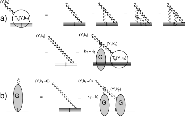
Refer to caption
Figure 17: Graphic form of equation for TA(y,kT)subscript𝑇𝐴𝑦subscript𝑘𝑇T_{A}\left(y,k_{T}\right). The wavy double lines denote T(Y,kT)𝑇𝑌subscript𝑘𝑇T\left(Y,k_{T}\right) of Eq. (51), while the wavy lines stand for TA(y,kT=0)subscript𝑇𝐴𝑦subscript𝑘𝑇0T_{A}\left(y,k_{T}=0\right).

Using Eq. (50) we can calculate C(|𝒑T1𝒑T2|)𝐶subscript𝒑𝑇1subscript𝒑𝑇2C\left(|\boldsymbol{p}_{T1}-\boldsymbol{p}_{T2}|\right) for proton-proton scattering, given by Eq. (1) which is equal to

Cpp(|𝒑T1𝒑T2|)=1Nc21d2kTT(kT,Yy1)T(kT,Yy2)T(𝒌T𝒑T,12,y1)T(𝒌T𝒑T,12,y2)d2kTT(kT,Yy1)T(kT,Yy2)T(kT,y1)T(kT,y2)subscript𝐶ppsubscript𝒑𝑇1subscript𝒑𝑇21subscriptsuperscript𝑁2𝑐1superscript𝑑2subscript𝑘𝑇𝑇subscript𝑘𝑇𝑌subscript𝑦1𝑇subscript𝑘𝑇𝑌subscript𝑦2𝑇subscript𝒌𝑇subscript𝒑𝑇12subscript𝑦1𝑇subscript𝒌𝑇subscript𝒑𝑇12subscript𝑦2superscript𝑑2subscript𝑘𝑇𝑇subscript𝑘𝑇𝑌subscript𝑦1𝑇subscript𝑘𝑇𝑌subscript𝑦2𝑇subscript𝑘𝑇subscript𝑦1𝑇subscript𝑘𝑇subscript𝑦2C_{\rm pp}\left(|\boldsymbol{p}_{T1}-\boldsymbol{p}_{T2}|\right)\,\,=\frac{1}{N^{2}_{c}-1}\frac{\,\int d^{2}k_{T}\,\,T\left(k_{T},Y-y_{1}\right)\,T\left(k_{T},Y-y_{2}\right)\,T\left(\boldsymbol{k}_{T}\,-\,\boldsymbol{p}_{T,12},y_{1}\right)\,T\left(\boldsymbol{k}_{T}\,-\,\boldsymbol{p}_{T,12},\ y_{2}\right)}{\,\int d^{2}k_{T}\,\,T\left(k_{T},Y-y_{1}\right)\,T\left(k_{T},Y-y_{2}\right)\,T\left(k_{T},y_{1}\right)\,T\left(k_{T},\ y_{2}\right)} (56)

For proton-nucleus we have

CpA(|𝒑T1𝒑T2|)=1Nc21d2kTTA(kT,Yy1)TA(kT,Yy2)T(𝒌T𝒑T,12,y1)T(𝒌T𝒑T,12,y2)d2kTT(kT,Yy1)T(kT,Yy2)T(kT,y1)T(kT,y2)subscript𝐶pAsubscript𝒑𝑇1subscript𝒑𝑇21subscriptsuperscript𝑁2𝑐1superscript𝑑2subscript𝑘𝑇subscript𝑇𝐴subscript𝑘𝑇𝑌subscript𝑦1subscript𝑇𝐴subscript𝑘𝑇𝑌subscript𝑦2𝑇subscript𝒌𝑇subscript𝒑𝑇12subscript𝑦1𝑇subscript𝒌𝑇subscript𝒑𝑇12subscript𝑦2superscript𝑑2subscript𝑘𝑇𝑇subscript𝑘𝑇𝑌subscript𝑦1𝑇subscript𝑘𝑇𝑌subscript𝑦2𝑇subscript𝑘𝑇subscript𝑦1𝑇subscript𝑘𝑇subscript𝑦2C_{\rm pA}\left(|\boldsymbol{p}_{T1}-\boldsymbol{p}_{T2}|\right)\,\,=\frac{1}{N^{2}_{c}-1}\frac{\,\int d^{2}k_{T}\,\,T_{A}\left(k_{T},Y-y_{1}\right)\,T_{A}\left(k_{T},Y-y_{2}\right)\,T\left(\boldsymbol{k}_{T}\,-\,\boldsymbol{p}_{T,12},y_{1}\right)\,T\left(\boldsymbol{k}_{T}\,-\,\boldsymbol{p}_{T,12},\ y_{2}\right)}{\,\int d^{2}k_{T}\,\,T\left(k_{T},Y-y_{1}\right)\,T\left(k_{T},Y-y_{2}\right)\,T\left(k_{T},y_{1}\right)\,T\left(k_{T},\ y_{2}\right)} (57)

and for nucleus - nucleus CAAsubscript𝐶AAC_{\rm AA} has the form:

CAA(|𝒑T1𝒑T2|)=1Nc21d2kTTA(kT,Yy1)TA(kT,Yy2)TA(𝒌T𝒑T,12,y1)TA(𝒌T𝒑T,12,y2)d2kTT(kT,Yy1)T(kT,Yy2)T(kT,y1)T(kT,y2)subscript𝐶AAsubscript𝒑𝑇1subscript𝒑𝑇21subscriptsuperscript𝑁2𝑐1superscript𝑑2subscript𝑘𝑇subscript𝑇𝐴subscript𝑘𝑇𝑌subscript𝑦1subscript𝑇𝐴subscript𝑘𝑇𝑌subscript𝑦2subscript𝑇𝐴subscript𝒌𝑇subscript𝒑𝑇12subscript𝑦1subscript𝑇𝐴subscript𝒌𝑇subscript𝒑𝑇12subscript𝑦2superscript𝑑2subscript𝑘𝑇𝑇subscript𝑘𝑇𝑌subscript𝑦1𝑇subscript𝑘𝑇𝑌subscript𝑦2𝑇subscript𝑘𝑇subscript𝑦1𝑇subscript𝑘𝑇subscript𝑦2C_{\rm AA}\left(|\boldsymbol{p}_{T1}-\boldsymbol{p}_{T2}|\right)\,\,=\frac{1}{N^{2}_{c}-1}\frac{\,\int d^{2}k_{T}\,\,T_{A}\left(k_{T},Y-y_{1}\right)\,T_{A}\left(k_{T},Y-y_{2}\right)\,T_{A}\left(\boldsymbol{k}_{T}\,-\,\boldsymbol{p}_{T,12},y_{1}\right)\,T_{A}\left(\boldsymbol{k}_{T}\,-\,\boldsymbol{p}_{T,12},\ y_{2}\right)}{\,\int d^{2}k_{T}\,\,T\left(k_{T},Y-y_{1}\right)\,T\left(k_{T},Y-y_{2}\right)\,T\left(k_{T},y_{1}\right)\,T\left(k_{T},\ y_{2}\right)} (58)

The results of calculations for C(RcorpT,12)𝐶subscript𝑅corsubscript𝑝𝑇12C\left(R_{\rm cor}p_{T,12}\right) using Eq. (56) - Eq. (58) are plotted in Fig. 18, One can see that the radius of correlations (Rcor2=Bsuperscriptsubscript𝑅cor2𝐵R_{\rm cor}^{2}=B) turns out to be very small in comparison with the same radius in Fig. 8 and Fig. 10.
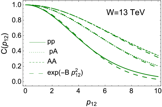
Refer to caption
Figure 18: C(|𝒑T1𝒑T2|=pT,12)𝐶subscript𝒑𝑇1subscript𝒑𝑇2subscript𝑝𝑇12C\left(|\boldsymbol{p}_{T1}-\boldsymbol{p}_{T2}|=p_{T,12}\right), calculated using Eq. (56) - Eq. (58), versus pT,12subscript𝑝𝑇12p_{T,12} for three reactions: proton-proton, proton - lead and lead - lead collisions at energy W=13TeV𝑊13𝑇𝑒𝑉W=13\,TeV. The long dashed curves correspond to exp(BpT,122)𝐵subscriptsuperscript𝑝2𝑇12\exp\left(-B\,p^{2}_{T,12}\right) with Bpp=0.035GeV2subscript𝐵pp0.035𝐺𝑒superscript𝑉2B_{\rm pp}=0.035\,GeV^{-2}, BpA=0.027Ge4V2subscript𝐵pA0.027𝐺𝑒4superscript𝑉2B_{\rm pA}=0.027\,Ge4V^{-2} and BAA=0.022GeV2subscript𝐵AA0.022𝐺𝑒superscript𝑉2B_{\rm AA}=0.022\,GeV^{-2}.

From C(RcorpT,12)𝐶subscript𝑅corsubscript𝑝𝑇12C\left(R_{\rm cor}p_{T,12}\right) we can calculate vnsubscript𝑣𝑛v_{n} using Eq. (11) and Eq. (12)-1. However, C(RcorpT,12)𝐶subscript𝑅corsubscript𝑝𝑇12C\left(R_{\rm cor}p_{T,12}\right) shown in Fig. 18, are calculated for the production of gluon jets, while experimentally vnsubscript𝑣𝑛v_{n} are measured for a hadron. Following Ref. LEREINC we explore the local parton-hadron duality(LPHD) suggested in Ref. LPHD .

In our approach the hadrons originate from the decay of a gluon jet, and their transverse momenta are

𝒑hadron,T=z𝒑jet,T+𝒑intristic,Tsubscript𝒑hadronT𝑧subscript𝒑jetTsubscript𝒑intristicT\boldsymbol{p}_{\rm hadron,\,T}\,=\,z\,\boldsymbol{p}_{\rm jet,\,T}\,\,+\,\,\boldsymbol{p}_{\rm intristic,\,T} (59)

where z𝑧z is the fraction of energy of the jet, carried by the hadron. 𝒑intristic,Tsubscript𝒑intristicT\boldsymbol{p}_{\rm intristic,\,T} is the transverse momentum of the hadron in the mini-jet that has only longitudinal momentum. From Eq. (59) we obtain that the average pTsubscript𝑝𝑇p_{T} of hadrons is equal to

phadron,T=z2pjet,T2+pintristic,T2delimited-⟨⟩subscript𝑝hadronTsuperscript𝑧2subscriptsuperscript𝑝2jetTsubscriptsuperscript𝑝2intristicT\langle p_{\rm hadron,\,T}\rangle\,\,=\,\,\sqrt{z^{2}\,p^{2}_{\rm jet,\,T}\,\,+\,\,p^{2}_{\rm intristic,\,T}} (60)

In Ref.LEREINC we found that we need to take z=0.5𝑧0.5z=0.5 and pintristic,T=mπsubscript𝑝intristicTsubscript𝑚𝜋p_{\rm intristic,\,T}=m_{\pi}, to describe the inclusive spectra of hadron at the LHC. Using Eq. (60) we recalculate vnsubscript𝑣𝑛v_{n} for a gluon jet to vnsubscript𝑣𝑛v_{n} for hadrons, which are shown in Fig. 19. Comparing with the experimental data CMSPP ; STARAA ; PHOBOSAA ; STARAA1 ; CMSPA ; CMSAA ; ALICEAA ; ALICEPA ; ATLASPP ; ATLASPA ; ATLASAA , and Fig. 7-b and Fig. 12, one can see that we describe the proton-proton scattering rather well, while for proton-nucleus we obtain v2subscript𝑣2v_{2} which is smaller by 15- 20%. For lead-lead collisions v2subscript𝑣2v_{2} turns out to be two times smaller than the experimental value ATLASAA . However, for central events with centrality 0 - 10% measured v2subscript𝑣2v_{2} is very close to our estimates. vnsubscript𝑣𝑛v_{n} with n3𝑛3n\geq 3 are larger than the experimental values. In general the pTsubscript𝑝𝑇p_{T} distribution is wider than the experimental one. The LPHD approach and Eq. (60) are very approximate, and we need to use a more advanced jet fragmentation function. Second, we need to add together the two mechanisms: one discussed in this section and one discussed in section 2. We need to include a more advanced fragmentation function, together with more careful accounting of the emission vertex in QCD (see appendix A). We will consider these in a future publication.
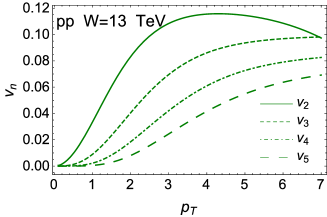
Refer to caption Refer to caption Refer to caption
Fig. 19-a Fig. 19-b Fig. 19-c
Figure 19: vnsubscript𝑣𝑛v_{n} versus pTsubscript𝑝𝑇p_{T} at W=13TeV𝑊13𝑇𝑒𝑉W=13\,TeV for proton-proton (Fig. 19-a), proton-lead (Fig. 19-b) and lead-lead (Fig. 19-c) scatterings, using Eq. (11) and Eq. (12)-1.

The estimates from our model show that the mechanism that has been discussed in section 2, yields about 10 -20% of the contribution which we now consider. In Fig. 20 one can see how the sum of two mechanism occur in v2subscript𝑣2v_{2}. One can see that the sum has a wider pTsubscript𝑝𝑇p_{T} distribution and a smaller maximal value. For proton-proton collisions both effects make predictions closer to the experimentally observed values of v2subscript𝑣2v_{2} ATLASPP .

Refer to caption Refer to caption
Fig. 20-a Fig. 20-b
Figure 20: v2subscript𝑣2v_{2} versus pTsubscript𝑝𝑇p_{T} at W=13TeV𝑊13𝑇𝑒𝑉W=13\,TeV for proton-proton (Fig. 20-a) and proton-lead (Fig. 20-b) for the sum of two contributions: the ‘dressed’ Pomeron structure and the diffractive production, discussed in section 2. The percents indicate the fraction of diffractive production in the Pomeron structure.

One of the properties that has been violated in the estimates in section 2, was the factorization rn=1subscript𝑟𝑛1r_{n}=1 where

rn=VnΔ(pT1,pT2)VnΔ(pT1,pT1)VnΔ(pT2,pT2)= 1subscript𝑟𝑛subscript𝑉𝑛Δsubscript𝑝𝑇1subscript𝑝𝑇2subscript𝑉𝑛Δsubscript𝑝𝑇1subscript𝑝𝑇1subscript𝑉𝑛Δsubscript𝑝𝑇2subscript𝑝𝑇21r_{n}\,=\,\frac{V_{n\Delta}\left(p_{T1},p_{T2}\right)}{\sqrt{V_{n\Delta}\left(p_{T1},p_{T1}\right)\,V_{n\Delta}\left(p_{T2},p_{T2}\right)}}\,=\,1 (61)

Fig. 21 shows that Eq. (61) holds at least for pT4GeVsubscript𝑝𝑇4𝐺𝑒𝑉p_{T}\leq 4\,GeV in accordance with the experimental data (see Ref.ATLASPA ).

Refer to caption Refer to caption Refer to caption Refer to caption
Fig. 21-a Fig. 21-b Fig. 21-c Fig. 21-d
Figure 21: The ration rnsubscript𝑟𝑛r_{n} versus pTsubscript𝑝𝑇p_{T} at W=5TeV𝑊5𝑇𝑒𝑉W=5\,TeV for proton-lead collisions. 

V Conclusions

In this paper we showed how three different dimensional scales in high energy scattering, arise in the Bose-Einstaein correlations that generates vnsubscript𝑣𝑛v_{n}, for even and odd n𝑛n. The first two scales are intimately related to the structure of the wave function of the hadron, and have an interpretation in the constituent quark model, as the distance between the constituent quarks and the size of the quark. In a more formal way they characterize the size of the vertex of the BFKL Pomeron interaction with the hadron, and the typical size of the same vertex for the diffraction production, in the region of small mass. We demonstrated that these sizes lead to BE correlations which are large, but narrowly distributed in pTsubscript𝑝𝑇p_{T} .

The third size is the value of the saturation momentum in the CGC/saturation approach, and has been used in the construction of our model for the high energy soft interactions. This size is incorporated in the structure of the ‘dressed’ Pomeron in our model. It turns out that this size leads to values of vnsubscript𝑣𝑛v_{n} which are close to the experimental values both for even and odd n𝑛n, and they are broadly distributed in pTsubscript𝑝𝑇p_{T}. In proton-proton scattering this mechanism is able to describe the experimental data both for even and odd vnsubscript𝑣𝑛v_{n}, while for proton-nucleus and nucleus-nucleus collisions we obtain smaller values of v2subscript𝑣2v_{2}: 20-30% smaller for proton-lead scattering, and two times smaller for lead-lead collisions. However, we would like to stress that for centrality 0-10%, the structure of the Pomeron gives values of vnsubscript𝑣𝑛v_{n} which are very close to the experimentally observed ones.

All estimates were made in the framework of our model for soft interactions which is based on CGC/saturation approach, but introduces non-perturbative parameters which describe the wave function of the hadron, and the large impact parameter behaviour of the saturation momentum. We describe in this model the total, elastic and diffractive cross sections as well as the inclusive production and long range rapidity correlations, and therefore, we trust that we can rely on the model when discussing the azimuthal angle correlations.

We demonstrated in this paper that BE correlations in the framework of CGC/saturation approach are able to explain a substantial part if not the entire, experimental values of vnsubscript𝑣𝑛v_{n} for both even and odd n𝑛n. Therefore, we believe that is premature to conclude that the origin of the observed long range rapidity correlations are only due to elliptic flow.

Acknowledgements We thank our colleagues at Tel Aviv University and UTFSM for encouraging discussions. Our special thanks go to Carlos Cantreras, Alex Kovner and Michel Lublinsky for elucidating discussions on the subject of this paper. This research was supported by the BSF grant 2012124, by Proyecto Basal FB 0821(Chile) , Fondecyt (Chile) grant 1140842 and by CONICYT grant PIA ACT1406.

Appendix A

A.1 BFKL contribution for the interference diagram

In this appendix we derive the BFKL contribution to dσdy1d2pT1(kT,|𝒌𝑻+𝒑T,12|)𝑑𝜎𝑑subscript𝑦1superscript𝑑2subscript𝑝𝑇1subscript𝑘𝑇subscript𝒌𝑻subscript𝒑𝑇12\frac{d\sigma}{dy_{1}d^{2}p_{T1}}\left(k_{T},|\boldsymbol{k_{T}}+\boldsymbol{p}_{T,12}|\right) given by Eq. (14).

Refer to caption
Figure 22: The graphical representation of Eq. (14).

The Lipatov vertices Γμ(qT,pT1)subscriptΓ𝜇subscript𝑞𝑇subscript𝑝𝑇1\Gamma_{\mu}\left(q_{T},p_{T1}\right) and Γμ(qT1,pT2)subscriptΓ𝜇subscript𝑞𝑇1subscript𝑝𝑇2\Gamma_{\mu}\left(q_{T1},p_{T2}\right) have the form (see book KOLEB for example):

Γμ(qT,pT1)=1pT12(qT2𝒑T1𝒒TpT12);Γμ(qT1,pT2)=1pT22(qT12𝒑T2𝒒T1pT22);formulae-sequencesubscriptΓ𝜇subscript𝑞𝑇subscript𝑝𝑇11superscriptsubscript𝑝𝑇12subscriptsuperscript𝑞2𝑇subscript𝒑𝑇1subscript𝒒𝑇subscriptsuperscript𝑝2𝑇1subscriptΓ𝜇subscript𝑞𝑇1subscript𝑝𝑇21superscriptsubscript𝑝𝑇22subscriptsuperscript𝑞2𝑇1subscript𝒑𝑇2subscript𝒒𝑇1subscriptsuperscript𝑝2𝑇2\Gamma_{\mu}\left(q_{T},p_{T1}\right)\,\,=\,\,\frac{1}{p_{T1}^{2}}\left(\,q^{2}_{T}\,\boldsymbol{p}_{T1}\,-\,\boldsymbol{q}_{T}\,p^{2}_{T1}\right);~{}~{}~{}~{}~{}~{}~{}~{}\Gamma_{\mu}\left(q_{T1},p_{T2}\right)\,\,=\,\,\frac{1}{p_{T2}^{2}}\left(\,q^{2}_{T1}\,\boldsymbol{p}_{T2}\,-\,\boldsymbol{q}_{T1}\,p^{2}_{T2}\right); (62)

and

Γμ(qT,pT1)Γμ(qT1,pT2)=qT12(𝒒T𝒑T2)2pT22+qT2(𝒒T1𝒑T1)2pT12kT2pT,122qT2qT12pT12pT22subscriptΓ𝜇subscript𝑞𝑇subscript𝑝𝑇1subscriptΓ𝜇subscript𝑞𝑇1subscript𝑝𝑇2subscriptsuperscript𝑞2𝑇1superscriptsubscript𝒒𝑇subscript𝒑𝑇22subscriptsuperscript𝑝2𝑇2subscriptsuperscript𝑞2𝑇superscriptsubscript𝒒𝑇1subscript𝒑𝑇12subscriptsuperscript𝑝2𝑇1subscriptsuperscript𝑘2𝑇subscriptsuperscript𝑝2𝑇12subscriptsuperscript𝑞2𝑇subscriptsuperscript𝑞2𝑇1subscriptsuperscript𝑝2𝑇1subscriptsuperscript𝑝2𝑇2\Gamma_{\mu}\left(q_{T},p_{T1}\right)\,\Gamma_{\mu}\left(q_{T1},p_{T2}\right)\,\,=\,\,\frac{q^{2}_{T1}\,\left(\boldsymbol{q}_{T}-\boldsymbol{p}_{T2}\right)^{2}}{p^{2}_{T2}}\,+\,\frac{q^{2}_{T}\,\left(\boldsymbol{q}_{T1}-\boldsymbol{p}_{T1}\right)^{2}}{p^{2}_{T1}}\,-\,k^{2}_{T}\,-\,p^{2}_{T,12}\frac{q^{2}_{T}\,q^{2}_{T1}}{p^{2}_{T1}\,p^{2}_{T2}} (63)

where 𝒑T,12=𝒑T1𝒑T2subscript𝒑𝑇12subscript𝒑𝑇1subscript𝒑𝑇2\boldsymbol{p}_{T,12}\,=\,\boldsymbol{p}_{T1}-\boldsymbol{p}_{T2} , 𝒒T=𝒒T𝒑T1subscriptsuperscript𝒒𝑇subscript𝒒𝑇subscript𝒑𝑇1\boldsymbol{q}^{\,{}^{\prime}}_{T}\,=\,\,\boldsymbol{q}_{T}-\boldsymbol{p}_{T1}, 𝒒T1=𝒒T1𝒑T2subscriptsuperscript𝒒𝑇1subscript𝒒𝑇1subscript𝒑𝑇2\boldsymbol{q}^{\,{}^{\prime}}_{T1}\,=\,\,\boldsymbol{q}_{T1}-\boldsymbol{p}_{T2}, and 𝒒T1=𝒒T𝒌Tsubscript𝒒𝑇1subscript𝒒𝑇subscript𝒌𝑇\boldsymbol{q}_{T1}=\boldsymbol{q}_{T}-\boldsymbol{k}_{T}. Eq. (63) can be re-written as

Γμ(qT,pT1)Γμ(qT1,pT2)=qT12(𝒒T+𝒑T,12)2pT22+qT2(𝒒T1𝒑T,12)2pT12kT2pT,122qT2qT12pT12pT22subscriptΓ𝜇subscript𝑞𝑇subscript𝑝𝑇1subscriptΓ𝜇subscript𝑞𝑇1subscript𝑝𝑇2subscriptsuperscript𝑞2𝑇1superscriptsubscriptsuperscript𝒒𝑇subscript𝒑𝑇122subscriptsuperscript𝑝2𝑇2subscriptsuperscript𝑞2𝑇superscriptsubscriptsuperscript𝒒𝑇1subscript𝒑𝑇122subscriptsuperscript𝑝2𝑇1subscriptsuperscript𝑘2𝑇subscriptsuperscript𝑝2𝑇12subscriptsuperscript𝑞2𝑇subscriptsuperscript𝑞2𝑇1subscriptsuperscript𝑝2𝑇1subscriptsuperscript𝑝2𝑇2\Gamma_{\mu}\left(q_{T},p_{T1}\right)\,\Gamma_{\mu}\left(q_{T1},p_{T2}\right)\,\,=\,\,\frac{q^{2}_{T1}\,\left(\boldsymbol{q}^{\,{}^{\prime}}_{T}+\boldsymbol{p}_{T,12}\right)^{2}}{p^{2}_{T2}}\,+\,\frac{q^{2}_{T}\,\left(\boldsymbol{q}^{\,{}^{\prime}}_{T1}-\boldsymbol{p}_{T,12}\right)^{2}}{p^{2}_{T1}}\,-\,k^{2}_{T}\,-\,p^{2}_{T,12}\frac{q^{2}_{T}\,q^{2}_{T1}}{p^{2}_{T1}\,p^{2}_{T2}} (64)

ϕBFKLsuperscriptitalic-ϕBFKL\phi^{\rm BFKL} satisfies the following equation:

ϕBFKL(Y;qT,kT)Y=α¯Sd2qTπK(kT,qT)ϕBFKL(Y;qT,kT)superscriptitalic-ϕBFKL𝑌subscript𝑞𝑇subscript𝑘𝑇𝑌subscript¯𝛼𝑆superscript𝑑2subscriptsuperscript𝑞𝑇𝜋𝐾subscript𝑘𝑇subscriptsuperscript𝑞𝑇superscriptitalic-ϕBFKL𝑌subscriptsuperscript𝑞𝑇subscript𝑘𝑇\frac{\partial\phi^{\rm BFKL}\left(Y;q_{T},k_{T}\right)}{\partial\,Y}\,\,=\,\,\bar{\alpha}_{S}\,\int\frac{d^{2}q^{\prime}_{T}}{\pi}\,K\left(k_{T},q^{\prime}_{T}\right)\,\phi^{\rm BFKL}\left(Y;q^{\prime}_{T},k_{T}\right) (65)

where

K(kT,qT)=𝐾subscript𝑘𝑇subscriptsuperscript𝑞𝑇absent\displaystyle K\left(k_{T},q^{\prime}_{T}\right)\,\,= (66)
(qT12qT2pT2+qT2qT12pT2kT2)1qT2qT12{qT2d2pTpT2(𝒒T𝒑T)2+qT2d2pTpT2(𝒒T𝒑T)2}δ(2)(𝒒t𝒒T)subscriptsuperscript𝑞2𝑇1subscriptsuperscript𝑞2𝑇subscriptsuperscript𝑝2𝑇subscriptsuperscript𝑞2𝑇subscriptsuperscript𝑞2𝑇1subscriptsuperscript𝑝2𝑇subscriptsuperscript𝑘2𝑇1subscriptsuperscript𝑞2𝑇subscriptsuperscript𝑞2𝑇1subscriptsuperscript𝑞2𝑇superscript𝑑2subscript𝑝𝑇subscriptsuperscript𝑝2𝑇superscriptsubscript𝒒𝑇subscript𝒑𝑇2subscriptsuperscript𝑞2𝑇superscript𝑑2subscript𝑝𝑇subscriptsuperscript𝑝2𝑇superscriptsubscriptsuperscript𝒒𝑇subscript𝒑𝑇2superscript𝛿2subscriptsuperscript𝒒𝑡subscript𝒒𝑇\displaystyle\,\,\Bigg{(}\frac{q^{2}_{T1}\,q^{\prime 2}_{T}}{p^{2}_{T}}\,+\,\frac{q^{2}_{T}\,q^{\prime 2}_{T1}}{p^{2}_{T}}\,-\,k^{2}_{T}\Bigg{)}\frac{1}{q^{\prime 2}_{T}\,q^{\prime 2}_{T1}}\,\,-\,\Bigg{\{}q^{2}_{T}\int\frac{d^{2}p_{T}}{p^{2}_{T}\,\left(\boldsymbol{q}_{T}-\boldsymbol{p}_{T}\right)^{2}}\,+\,q^{\prime 2}_{T}\int\frac{d^{2}p_{T}}{p^{2}_{T}\,\left(\boldsymbol{q}^{\,{}^{\prime}}_{T}-\boldsymbol{p}_{T}\right)^{2}}\Bigg{\}}\delta^{(2)}\left(\boldsymbol{q}^{\,{}^{\prime}}_{t}-\boldsymbol{q}_{T}\right)

Eq. (65) is the BFKL equation in the momentum representation, which has the following form in the coordinate representationLI ; MUCD :

NBFKL(Y;x12,b)Y=superscript𝑁BFKL𝑌subscript𝑥12𝑏𝑌absent\displaystyle\frac{\partial N^{\rm BFKL}\left(Y;x_{12},b\right)}{\partial\,Y}\,\,= (67)
α¯Sd2x3πx122x132x232{N(Y;x13,𝒃12𝒙23)+N(Y;x23,𝒃12𝒙13)N(Y;x13,b)}subscript¯𝛼𝑆superscript𝑑2subscript𝑥3𝜋subscriptsuperscript𝑥212subscriptsuperscript𝑥213subscriptsuperscript𝑥223𝑁𝑌subscript𝑥13𝒃12subscript𝒙23𝑁𝑌subscript𝑥23𝒃12subscript𝒙13𝑁𝑌subscript𝑥13𝑏\displaystyle\,\,\bar{\alpha}_{S}\,\int\frac{d^{2}x_{3}}{\pi}\,\frac{x^{2}_{12}}{x^{2}_{13}\,x^{2}_{23}}\Big{\{}N\left(Y;x_{13},\boldsymbol{b}-\frac{1}{2}\boldsymbol{x}_{23}\right)\,+\,N\left(Y;x_{23},\boldsymbol{b}-\frac{1}{2}\boldsymbol{x}_{13}\right)\,-\,N\left(Y;x_{13},b\right)\Big{\}}

whereKOLEB ; KOTUINC

1(𝒒T+12𝒌T)2(12𝒌T𝒒T)2ϕBFKL(qT,kT)=2CFα¯S(2π)3d2bd2x12ei𝒒T𝒙12+i𝒌T𝒃NBFKL(Y;x12,b)1superscriptsubscript𝒒𝑇12subscript𝒌𝑇2superscript12subscript𝒌𝑇subscript𝒒𝑇2superscriptitalic-ϕBFKLsubscript𝑞𝑇subscript𝑘𝑇2subscript𝐶𝐹subscript¯𝛼𝑆superscript2𝜋3superscript𝑑2𝑏superscript𝑑2subscript𝑥12superscript𝑒𝑖subscript𝒒𝑇subscript𝒙12𝑖subscript𝒌𝑇𝒃superscript𝑁BFKL𝑌subscript𝑥12𝑏\frac{1}{\left(\boldsymbol{q}_{T}+\frac{1}{2}\boldsymbol{k}_{T}\right)^{2}\,\left(\frac{1}{2}\boldsymbol{k}_{T}-\boldsymbol{q}_{T}\right)^{2}}\phi^{\rm BFKL}\left(q_{T},k_{T}\right)\,\,=\,\,\frac{2\,C_{F}}{\bar{\alpha}_{S}(2\pi)^{3}}\int d^{2}b\,d^{2}x_{12}\,e^{i\boldsymbol{q}_{T}\cdot\boldsymbol{x}_{12}\,+\,i\boldsymbol{k}_{T}\cdot\boldsymbol{b}}\,N^{\rm BFKL}\left(Y;x_{12},b\right) (68)

For diagrams Fig. 2- c and Fig. 2-d 𝒑12=0subscript𝒑120\boldsymbol{p}_{12}=0 and plugging Eq. (68) in Eq. (14) we obtain that

dσdy1d2pT1(kT,kT)=(2CFα¯S(2π)3)2d2x12d2bd2bei𝒑T1𝒙12+i𝒌T𝒃𝑑𝜎𝑑subscript𝑦1superscript𝑑2subscript𝑝𝑇1subscript𝑘𝑇subscript𝑘𝑇superscript2subscript𝐶𝐹subscript¯𝛼𝑆superscript2𝜋32superscript𝑑2subscript𝑥12superscript𝑑2𝑏superscript𝑑2superscript𝑏superscript𝑒𝑖subscript𝒑𝑇1subscript𝒙12𝑖subscript𝒌𝑇𝒃\displaystyle\frac{d\sigma}{dy_{1}d^{2}p_{T1}}\left(k_{T},k_{T}\right)\,\,=\,\,\,\left(\frac{2\,C_{F}}{\bar{\alpha}_{S}(2\pi)^{3}}\right)^{2}\int d^{2}x_{12}\,d^{2}b\,d^{2}b^{\prime}\,e^{i\boldsymbol{p}_{T1}\cdot\boldsymbol{x}_{12}\,+\,i\boldsymbol{k}_{T}\cdot\boldsymbol{b}} (69)
×{1pT12(((12b+x12)2NBFKL(Yy;x12,𝒃𝒃))((12bx12)2NBFKL(y;x12,𝒃))\displaystyle\times\Bigg{\{}\frac{1}{p_{T1}^{2}}\left(\left(\left(\frac{1}{2}\boldsymbol{\nabla}_{b}\,+\,\boldsymbol{\nabla}_{x_{12}}\right)^{2}N^{\rm BFKL}\left(Y-y;x_{12},\boldsymbol{b}-\boldsymbol{b}^{\prime}\right)\right)\,\left(\left(\frac{1}{2}\boldsymbol{\nabla}_{b^{\prime}}\,-\,\boldsymbol{\nabla}_{x_{12}}\right)^{2}\,N^{\rm BFKL}\left(y;x_{12},\boldsymbol{b}^{\prime}\right)\right)\,\right.
+((12bx12)2NBFKL(Yy;x12,𝒃𝒃))((12b+x12)2NBFKL(y;x12,𝒃)))\displaystyle\left.+\,\left(\left(\frac{1}{2}\boldsymbol{\nabla}_{b}\,-\,\boldsymbol{\nabla}_{x_{12}}\right)^{2}N^{\rm BFKL}\left(Y-y;x_{12},\boldsymbol{b}-\boldsymbol{b}^{\prime}\right)\right)\,\left(\left(\frac{1}{2}\boldsymbol{\nabla}_{b^{\prime}}\,+\,\boldsymbol{\nabla}_{x_{12}}\right)^{2}\,N^{\rm BFKL}\left(y;x_{12},\boldsymbol{b}^{\prime}\right)\right)\right)
(bNBFKL(Yy;x12,𝒃𝒃))(bNBFKL(y;x12,𝒃))}\displaystyle\,-\,\left(\boldsymbol{\nabla}_{b}N^{\rm BFKL}\left(Y-y;x_{12},\boldsymbol{b}-\boldsymbol{b}^{\prime}\right)\right)\cdot\left(\boldsymbol{\nabla}_{b^{\prime}}N^{\rm BFKL}\left(y;x_{12},\boldsymbol{b}^{\prime}\right)\right)\Bigg{\}}

Eq. (69) in the limit kT0subscript𝑘𝑇0k_{T}\to 0, degenerates to the expression for the inclusive cross section which has the elegant form derived in Ref.KOTUINC

dσdy1d2pT1(kT=0,kT=0)=𝑑𝜎𝑑subscript𝑦1superscript𝑑2subscript𝑝𝑇1formulae-sequencesubscript𝑘𝑇0subscript𝑘𝑇0absent\displaystyle\frac{d\sigma}{dy_{1}d^{2}p_{T1}}\left(k_{T}=0,k_{T}=0\right)\,\,= (70)
(2CFα¯S(2π)3)21pT12d2x12ei𝒑T1x12(x122d2bNBFKL(Yy;x12,𝒃))(x122d2bNBFKL(y;x12,𝒃))superscript2subscript𝐶𝐹subscript¯𝛼𝑆superscript2𝜋321subscriptsuperscript𝑝2𝑇1superscript𝑑2subscript𝑥12superscript𝑒𝑖subscript𝒑𝑇1subscript𝑥12subscriptsuperscript2subscript𝑥12superscript𝑑2𝑏superscript𝑁BFKL𝑌𝑦subscript𝑥12𝒃subscriptsuperscript2subscript𝑥12superscript𝑑2superscript𝑏superscript𝑁BFKL𝑦subscript𝑥12superscript𝒃\displaystyle\left(\frac{2\,C_{F}}{\bar{\alpha}_{S}(2\pi)^{3}}\right)^{2}\frac{1}{p^{2}_{T1}}\,\int d^{2}x_{12}\,e^{i\boldsymbol{p}_{T1}\cdot x_{12}}\left(\nabla^{2}_{x_{12}}\int d^{2}b\,N^{\rm BFKL}\left(Y-y;x_{12},\boldsymbol{b}\right)\right)\,\left(\nabla^{2}_{x_{12}}\int d^{2}b^{\prime}\,N^{\rm BFKL}\left(y;x_{12},\boldsymbol{b}^{\prime}\right)\right)

The interesting feature of Eq. (69) and Eq. (70) is, that they remain correct, if we replace 2NBFKL2superscript𝑁BFKL2N^{\rm BFKL} by NG= 2NN2subscript𝑁𝐺2𝑁superscript𝑁2N_{G}\,=\,2\,N\,-\,N^{2}, where N𝑁N is the solution of the Balitsky-Kovchegov equationBK . Inside the saturation domain where N1𝑁1N\to 1, both equations lead to negligible contributions. In other words, in both equations the main contributions stem from the vicinity of the saturation scale, where x122Qs2 1subscriptsuperscript𝑥212subscriptsuperscript𝑄2𝑠1x^{2}_{12}\,Q^{2}_{s}\approx\,1.

The solution for the scattering amplitude of two dipoles r1subscript𝑟1r_{1} and r2subscript𝑟2r_{2} to Eq. (67) is knownLI

NIP(r1,r2;Y,b)=subscript𝑁𝐼𝑃subscript𝑟1subscript𝑟2𝑌𝑏absent\displaystyle N_{I\!\!P}\left(r_{1},r_{2};Y,b\right)\,\,= (71)
n=0dγ2πiϕin(n)(γ;r2)d2R1d2R2δ(𝑹1𝑹2𝒃)eω(γ,n)YEγ,n(r1,R1)E1γ,n(r2,R2)superscriptsubscript𝑛0𝑑𝛾2𝜋𝑖subscriptsuperscriptitalic-ϕ𝑛𝑖𝑛𝛾subscript𝑟2superscript𝑑2subscript𝑅1superscript𝑑2subscript𝑅2𝛿subscript𝑹1subscript𝑹2𝒃superscript𝑒𝜔𝛾𝑛𝑌superscript𝐸𝛾𝑛subscript𝑟1subscript𝑅1superscript𝐸1𝛾𝑛subscript𝑟2subscript𝑅2\displaystyle\,\,\sum_{n=0}^{\infty}\int\frac{d\gamma}{2\,\pi\,i}\,\phi^{(n)}_{in}(\gamma;r_{2})\,\,d^{2}\,R_{1}\,\,d^{2}\,R_{2}\,\delta(\boldsymbol{R}_{1}-\boldsymbol{R}_{2}-\boldsymbol{b})\,e^{\omega(\gamma,n)\,Y}\,E^{\gamma,n}\left(r_{1},R_{1}\right)\,E^{1-\gamma,n}\left(r_{2},R_{2}\right)

where the functions ϕin(n)(γ;r2)subscriptsuperscriptitalic-ϕ𝑛𝑖𝑛𝛾subscript𝑟2\phi^{(n)}_{in}(\gamma;r_{2}) are determined by the initial conditions at low energies and

ω(γ,n)=α¯Sχ(γ,n)=α¯S(2ψ(1)ψ(γ+|n|/2)ψ(1γ+|n|/2));𝜔𝛾𝑛subscript¯𝛼𝑆𝜒𝛾𝑛subscript¯𝛼𝑆2𝜓1𝜓𝛾𝑛2𝜓1𝛾𝑛2\omega(\gamma,n)\,\,=\,\,\bar{\alpha}_{S}\chi(\gamma,n)\,\,=\,\,\bar{\alpha}_{S}\left(2\psi\left(1\right)\,-\,\psi\left(\gamma+|n|/2\right)\,\,-\,\,\psi\left(1-\gamma+|n|/2\right)\right); (72)

where ψ(γ)=dlnΓ(γ)/dγ𝜓𝛾𝑑Γ𝛾𝑑𝛾~{}\psi\left(\gamma\right)\,\,=\,\,d\ln\Gamma\left(\gamma\right)/d\gamma and Γ(γ)Γ𝛾\Gamma\left(\gamma\right) is Euler gamma function. Functions En,γ(ρ1a,ρ2a)superscript𝐸𝑛𝛾subscript𝜌1𝑎subscript𝜌2𝑎E^{n,\gamma}\left(\rho_{1a},\rho_{2a}\right) are given by the following equations.

En,γ(ρ1a,ρ2a)=(ρ12ρ1aρ2a)1γ+n/2(ρ12ρ1aρ2a)1γn/2,superscript𝐸𝑛𝛾subscript𝜌1𝑎subscript𝜌2𝑎superscriptsubscript𝜌12subscript𝜌1𝑎subscript𝜌2𝑎1𝛾𝑛2superscriptsubscriptsuperscript𝜌12subscriptsuperscript𝜌1𝑎subscriptsuperscript𝜌2𝑎1𝛾𝑛2\displaystyle E^{n,\gamma}\left(\rho_{1a},\rho_{2a}\right)\,=\,\left(\frac{\rho_{12}}{\rho_{1a}\,\rho_{2a}}\right)^{1-\gamma+n/2}\,\left(\frac{\rho^{*}_{12}}{\rho^{*}_{1a}\,\rho^{*}_{2a}}\right)^{1-\gamma-n/2}, (73)

In Eq. (73) we use complex numbers to characterize the point on the plane

ρi=xi,1+ixi,2;ρi=xi,1ixi,2formulae-sequencesubscript𝜌𝑖subscript𝑥𝑖1𝑖subscript𝑥𝑖2subscriptsuperscript𝜌𝑖subscript𝑥𝑖1𝑖subscript𝑥𝑖2\displaystyle\rho_{i}=x_{i,1}+i\,x_{i,2};\,\,\,\,\,\,\,\rho^{*}_{i}=x_{i,1}-i\,x_{i,2} (74)

where the indices 111 and 222 denote two transverse axes. Note that

ρ12ρ12=ri2;ρ1aρ1a=(𝑹i12𝒓i)2ρ2aρ2a=(𝑹i+12𝒓i)2formulae-sequencesubscript𝜌12subscriptsuperscript𝜌12subscriptsuperscript𝑟2𝑖formulae-sequencesubscript𝜌1𝑎subscriptsuperscript𝜌1𝑎superscriptsubscript𝑹𝑖12subscript𝒓𝑖2subscript𝜌2𝑎subscriptsuperscript𝜌2𝑎superscriptsubscript𝑹𝑖12subscript𝒓𝑖2\rho_{12}\,\rho^{*}_{12}\,\,=\,\,r^{2}_{i};~{}~{}~{}~{}~{}~{}\rho_{1a}\,\rho^{*}_{1a}\,=\,\left(\boldsymbol{R}_{i}\,-\,\frac{1}{2}\boldsymbol{r}_{i}\right)^{2}~{}~{}~{}~{}~{}~{}\rho_{2a}\,\rho^{*}_{2a}\,=\,\left(\boldsymbol{R}_{i}\,+\,\frac{1}{2}\boldsymbol{r}_{i}\right)^{2} (75)

At large values of Y𝑌Y, the main contribution stems from the first term with n=0𝑛0n=0. For this term, Eq. (73) can be re-written in the form

Eγ,0(ri,Ri)=(ri2(𝑹i+12𝒓i)2(𝑹i12𝒓i)2)1γ.superscript𝐸𝛾0subscript𝑟𝑖subscript𝑅𝑖superscriptsubscriptsuperscript𝑟2𝑖superscriptsubscript𝑹𝑖12subscript𝒓𝑖2superscriptsubscript𝑹𝑖12subscript𝒓𝑖21𝛾E^{\gamma,0}\left(r_{i},R_{i}\right)\,\,=\,\,\left(\,\frac{r^{2}_{i}}{(\boldsymbol{R}_{i}\,+\,\frac{1}{2}\boldsymbol{r}_{i})^{2}\,\,(\boldsymbol{R}_{i}\,-\,\frac{1}{2}\boldsymbol{r}_{i})^{2}}\,\right)^{1-\gamma}\,\,. (76)

The integrals over R1subscript𝑅1R_{1} and R2subscript𝑅2R_{2} were taken in Refs.LI ; NAPE and at n=0𝑛0n=0 we have

Hγ(w,w)d2R1Eγ,0(r1,R1)E1γ,0(r2,𝑹1𝒃)=superscript𝐻𝛾𝑤superscript𝑤superscript𝑑2subscript𝑅1superscript𝐸𝛾0subscript𝑟1subscript𝑅1superscript𝐸1𝛾0subscript𝑟2subscript𝑹1𝒃absent\displaystyle H^{\gamma}\left(w,w^{*}\right)\,\,\equiv\,\,\int d^{2}\,R_{1}\,E^{\gamma,0}\left(r_{1},R_{1}\right)\,E^{1-\gamma,0}\left(r_{2},\boldsymbol{R}_{1}\,-\,\boldsymbol{b}\right)\,= (77)
(γ12)2(γ(1γ))2{bγwγwγF(γ,γ,2γ,w)F(γ,γ,2γ,w)\displaystyle\,\frac{(\gamma-\frac{1}{2})^{2}}{(\gamma(1-\gamma))^{2}}\Big{\{}b_{\gamma}\,w^{\gamma}\,{w^{*}}^{\gamma}\,F\left(\gamma,\gamma,2\gamma,w\right)\,F\left(\gamma,\gamma,2\gamma,w^{*}\right)
+b1γw1γw1γF(1γ,1γ,22γ,w)F(1γ,1γ,22γ,w)}\displaystyle\,+b_{1-\gamma}w^{1-\gamma}{w^{*}}^{1-\gamma}F\left(1-\gamma,1-\gamma,2-2\gamma,w\right)\,F\left(1-\gamma,1-\gamma,2-2\gamma,w^{*}\right)\Big{\}}
br1and/orr2(γ12)2(γ(1γ))2{bγwγwγ+b1γw1γw1γ}=(γ12)2(γ(1γ))2{bγ(r12r22b4)γ+b1γ(r12r22b4)1γ}much-greater-than𝑏subscript𝑟1and/orsubscript𝑟2absentsuperscript𝛾122superscript𝛾1𝛾2subscript𝑏𝛾superscript𝑤𝛾superscriptsuperscript𝑤𝛾subscript𝑏1𝛾superscript𝑤1𝛾superscriptsuperscript𝑤1𝛾superscript𝛾122superscript𝛾1𝛾2subscript𝑏𝛾superscriptsubscriptsuperscript𝑟21subscriptsuperscript𝑟22superscript𝑏4𝛾subscript𝑏1𝛾superscriptsubscriptsuperscript𝑟21subscriptsuperscript𝑟22superscript𝑏41𝛾\displaystyle\xrightarrow{b\,\gg\,r_{1}\,\,\mbox{\small and/or}\,\,r_{2}}\,\,\,\frac{(\gamma-\frac{1}{2})^{2}}{(\gamma(1-\gamma))^{2}}\Big{\{}b_{\gamma}\,w^{\gamma}\,{w^{*}}^{\gamma}\,+b_{1-\gamma}w^{1-\gamma}{w^{*}}^{1-\gamma}\Big{\}}\,=\,\,\frac{(\gamma-\frac{1}{2})^{2}}{(\gamma(1-\gamma))^{2}}\Big{\{}b_{\gamma}\,\left(\frac{r^{2}_{1}\,r^{2}_{2}}{b^{4}}\right)^{\gamma}\,+b_{1-\gamma}\left(\frac{r^{2}_{1}\,r^{2}_{2}}{b^{4}}\right)^{1-\gamma}\Big{\}}

where F𝐹F is hypergeometric function RY . In Eq. (77) ww𝑤superscript𝑤w\,w^{*} and bγsubscript𝑏𝛾b_{\gamma} are equal

ww=r12r22(𝒃12(𝒓1𝒓2))2(𝒃+12(𝒓1𝒓2))2;bγ=π3 24(1/2γ)Γ(γ)Γ(1/2γ)Γ(1γ)Γ(1/2+γ).formulae-sequence𝑤superscript𝑤subscriptsuperscript𝑟21subscriptsuperscript𝑟22superscript𝒃12subscript𝒓1subscript𝒓22superscript𝒃12subscript𝒓1subscript𝒓22subscript𝑏𝛾superscript𝜋3superscript2412𝛾Γ𝛾Γ12𝛾Γ1𝛾Γ12𝛾w\,w^{*}\,\,=\,\,\frac{r^{2}_{1}\,r^{2}_{2}}{\left(\boldsymbol{b}-\frac{1}{2}\left(\,\boldsymbol{r}_{1}\,-\,\boldsymbol{r}_{2}\right)\right)^{2}\,\left(\boldsymbol{b}\,+\,\frac{1}{2}\left(\,\boldsymbol{r}_{1}\,-\,\boldsymbol{r}_{2}\right)\right)^{2}};~{}~{}~{}~{}~{}~{}~{}~{}b_{\gamma}\,=\,\pi^{3}\,2^{4(1/2-\gamma)}\,\frac{\Gamma\left(\gamma\right)}{\Gamma\left(1/2-\gamma\right)}\,\frac{\Gamma\left(1-\gamma\right)}{\Gamma\left(1/2+\gamma\right)}. (78)

Therefore, at large b𝑏b, NBFKLsuperscript𝑁BFKLN^{\rm BFKL} decreases as a power of b𝑏b which violates the Froissart theorem KOWE . At present, as has been mentioned above, we cannot suggest a modification of the equation of the CGC/saturation approach in which the correctFROI exponential behaviour at large b𝑏b would be incorporated. So we doomed to build a model. We discussed our model in section 3.

A.2 Born diagrams

The spirited discussions with our colleagues, showed us that it would be benificial to add a general discussion of the BFKL contribution, by calculating of the first Born diagrams for the production of two identical gluons that have rapidities y1subscript𝑦1y_{1} and y2subscript𝑦2y_{2}, and carry momenta 𝒑T1subscript𝒑𝑇1\boldsymbol{p}_{T1} and 𝒑T2subscript𝒑𝑇2\boldsymbol{p}_{T2}. These diagrams are shown in Fig. 23 for the scattering of the bound states of two oniums (two dipoles). Such a model for the scattering systems allows us to use the perturbative QCD approach, and has the analogy in the simplest bound system: deuteron.

The two onium bound state is described by the wave function Ψ(𝑹1𝑹2)Ψsubscript𝑹1subscript𝑹2\Psi\left(\boldsymbol{R}_{1}-\boldsymbol{R}_{2}\right), where Risubscript𝑅𝑖R_{i} is the coordinate of the onium which is equal 𝑹i=12(𝒙i+𝒚i)subscript𝑹𝑖12subscript𝒙𝑖subscript𝒚𝑖\boldsymbol{R}_{i}=\frac{1}{2}\left(\boldsymbol{x}_{i}+\boldsymbol{y}_{i}\right) where 𝒙isubscript𝒙𝑖\boldsymbol{x}_{i} and 𝒚isubscript𝒚𝑖\boldsymbol{y}_{i} are coordinates of quark and antiquark in the onium (see Fig. 23). We introduce two new functions that describe the form factor of our bound state (G(q)𝐺𝑞G\left(q\right)), and the interaction of two gluons with the onium:

G(q)𝐺𝑞\displaystyle G\left(q\right)\, =\displaystyle= d2R|Ψ(R)|2ei𝒒𝑹with𝑹=𝑹1𝑹2;superscript𝑑2𝑅superscriptΨ𝑅2superscript𝑒𝑖𝒒𝑹with𝑹subscript𝑹1subscript𝑹2\displaystyle\,\int d^{2}R\,|\Psi\left(R\right)|^{2}\,\,e^{i\,\boldsymbol{q}\cdot\boldsymbol{R}}~{}~{}~{}\mbox{with}~{}~{}~{}\boldsymbol{R}=\boldsymbol{R}_{1}-\boldsymbol{R}_{2};
ϕonium(q,k)subscriptitalic-ϕonium𝑞𝑘\displaystyle\phi_{\rm onium}\left(q,k\right)\, =\displaystyle=  2d2ri|ψonium(ri)|2ei12𝒌𝒓i(1+ei𝒒𝒓i)with𝒓i=𝒙i𝒚i;2superscript𝑑2subscript𝑟𝑖superscriptsubscript𝜓oniumsubscript𝑟𝑖2superscript𝑒𝑖12𝒌subscript𝒓𝑖1superscript𝑒𝑖𝒒subscript𝒓𝑖withsubscript𝒓𝑖subscript𝒙𝑖subscript𝒚𝑖\displaystyle\,2\,\int d^{2}r_{i}\,|\psi_{\rm onium}\left(r_{i}\right)|^{2}\,\,e^{i\,\frac{1}{2}\boldsymbol{k}\cdot\boldsymbol{r}_{i}}\left(1+e^{i\boldsymbol{q}\cdot\boldsymbol{r}_{i}}\right)~{}~{}~{}~{}~{}\mbox{with}~{}~{}~{}~{}~{}\boldsymbol{r}_{i}\,=\,\boldsymbol{x}_{i}\,-\,\boldsymbol{y}_{i}; (79)

The contribution of the diagram of Fig. 23 can be written as222 We omit all numerical factors as well as α¯S6superscriptsubscript¯𝛼𝑆6\bar{\alpha}_{S}^{6}.

σinterferenced2k4π2G(k)G(𝒌+𝒑T,12)I2(𝒌,𝒑T1,𝒑T2)proportional-tosubscript𝜎interferencesuperscript𝑑2𝑘4superscript𝜋2𝐺𝑘𝐺𝒌subscript𝒑𝑇12superscript𝐼2𝒌subscript𝒑𝑇1subscript𝒑𝑇2\sigma_{\rm interference}\,\propto\,\int\frac{d^{2}k}{4\pi^{2}}\,G\left(k\right)\,G\left(\boldsymbol{k}+\boldsymbol{p}_{T,12}\right)\,I^{2}\left(\boldsymbol{k},\boldsymbol{p}_{T1},\boldsymbol{p}_{T2}\right) (80)

where

I(𝒌,𝒑T1,𝒑T2)𝐼𝒌subscript𝒑𝑇1subscript𝒑𝑇2\displaystyle I\left(\boldsymbol{k},\boldsymbol{p}_{T1},\boldsymbol{p}_{T2}\right)\, proportional-to\displaystyle\propto d2q4π2ϕonium(𝒌,𝒒)ϕonium(𝒌𝒑T,12,𝒒)superscript𝑑2𝑞4superscript𝜋2subscriptitalic-ϕonium𝒌𝒒subscriptitalic-ϕonium𝒌subscript𝒑𝑇12𝒒\displaystyle\,\int\frac{d^{2}q}{4\,\pi^{2}}\,\,\phi_{\rm onium}\left(\boldsymbol{k},\boldsymbol{q}\right)\,\phi_{\rm onium}\left(\boldsymbol{k}\,-\,\boldsymbol{p}_{T,12},\boldsymbol{q}\right)\, (81)
×\displaystyle\times {1q2(𝒌𝒒)2Γμ(qT,pT1)Γμ(qT1,pT2)1(𝒒𝒑T1)2(𝒌𝒑T,12𝒒)2}1superscript𝑞2superscript𝒌𝒒2subscriptΓ𝜇subscript𝑞𝑇subscript𝑝𝑇1subscriptΓ𝜇subscript𝑞𝑇1subscript𝑝𝑇21superscript𝒒subscript𝒑𝑇12superscript𝒌subscript𝒑𝑇12𝒒2\displaystyle\Bigg{\{}\frac{1}{q^{2}\,\left(\boldsymbol{k}-\boldsymbol{q}\right)^{2}}\,\Gamma_{\mu}\left(q_{T},p_{T1}\right)\,\Gamma_{\mu}\left(q_{T1},p_{T2}\right)\,\,\frac{1}{\left(\boldsymbol{q}-\boldsymbol{p}_{T1}\right)^{2}\,\left(\boldsymbol{k}-\boldsymbol{p}_{T,12}-\boldsymbol{q}\right)^{2}}\Bigg{\}}

where Γμ(qT,pT1)Γμ(qT1,pT2)subscriptΓ𝜇subscript𝑞𝑇subscript𝑝𝑇1subscriptΓ𝜇subscript𝑞𝑇1subscript𝑝𝑇2\Gamma_{\mu}\left(q_{T},p_{T1}\right)\,\Gamma_{\mu}\left(q_{T1},p_{T2}\right) is given by Eq. (63) and Eq. (64).

One can see from Eq. (80) and Eq. (3) that the typical q1/r𝑞1𝑟q\approx 1/r, where r𝑟r is he size of the onium , while the typical values of k1/Rproportional-to𝑘1𝑅k\propto 1/R, where R𝑅R is the size of the bound state. Assuming that Rrmuch-greater-than𝑅𝑟R\gg r, we see that kqmuch-less-than𝑘𝑞k\,\ll\,q. Anticipating pT,121/Rproportional-tosubscript𝑝𝑇121𝑅p_{T,12}\propto 1/R, we can reduce the contribution of the interference diagram to the following form:

σinterference1pT12pT,22d2k4π2G(k)G(𝒌+𝒑T,12)(d2q4π21q2(𝒒𝒑T1)2)2proportional-tosubscript𝜎interference1subscriptsuperscript𝑝2𝑇1subscriptsuperscript𝑝2𝑇2superscript𝑑2𝑘4superscript𝜋2𝐺𝑘𝐺𝒌subscript𝒑𝑇12superscriptsuperscript𝑑2𝑞4superscript𝜋21superscript𝑞2superscript𝒒subscript𝒑𝑇122\sigma_{\rm interference}\,\propto\,\frac{1}{p^{2}_{T1}\,p^{2}_{T,2}}\int\frac{d^{2}k}{4\pi^{2}}\,G\left(k\right)\,G\left(\boldsymbol{k}+\boldsymbol{p}_{T,12}\right)\Bigg{(}\int\frac{d^{2}q}{4\pi^{2}}\frac{1}{q^{2}\,\left(\boldsymbol{q}-\boldsymbol{p}_{T1}\right)^{2}}\Bigg{)}^{2} (82)

In Eq. (82) we assume that pT1pT2subscript𝑝𝑇1subscript𝑝𝑇2p_{T1}\approx p_{T2} and one can see that pT,12subscript𝑝𝑇12p_{T,12} from this equation is indeed of the order of 1/R1𝑅1/R, being much smaller than pTisubscript𝑝𝑇𝑖p_{Ti} if they are of the order of 1/r1𝑟1/r. For 1/RpTi 1/rmuch-less-than1𝑅subscript𝑝𝑇𝑖much-less-than1𝑟1/R\,\ll\,p_{Ti}\,\ll\,1/r we need to take Γμ(qT,pT1)Γμ(qT1,pT2)=(1pT12+1pT22)1q4subscriptΓ𝜇subscript𝑞𝑇subscript𝑝𝑇1subscriptΓ𝜇subscript𝑞𝑇1subscript𝑝𝑇21subscriptsuperscript𝑝2𝑇11subscriptsuperscript𝑝2𝑇21superscript𝑞4\Gamma_{\mu}\left(q_{T},p_{T1}\right)\,\Gamma_{\mu}\left(q_{T1},p_{T2}\right)\,\,=\,\,\left(\frac{1}{p^{2}_{T1}}\,+\,\frac{1}{p^{2}_{T2}}\right)\,\frac{1}{q^{4}}.

Refer to caption
Figure 23: The Born interference diagram for production of two identical gluons with rapidities:y1subscript𝑦1y_{1} and y2subscript𝑦2y_{2} and transverse momenta 𝒑T1subscript𝒑𝑇1\boldsymbol{p}_{T1} and 𝒑T2subscript𝒑𝑇2\boldsymbol{p}_{T2}.𝑹i=12(𝒙i+𝒚i)subscript𝑹𝑖12subscript𝒙𝑖subscript𝒚𝑖\boldsymbol{R}_{i}=\frac{1}{2}\left(\boldsymbol{x}_{i}+\boldsymbol{y}_{i}\right), 𝒑T,12=𝒑T1𝒑T2subscript𝒑𝑇12subscript𝒑𝑇1subscript𝒑𝑇2\boldsymbol{p}_{T,12}=\boldsymbol{p}_{T1}-\boldsymbol{p}_{T2}. Red rectangle shows function Φ(𝒌,𝒑T1,𝒑T2)Φ𝒌subscript𝒑𝑇1subscript𝒑𝑇2\Phi\left(\boldsymbol{k},\boldsymbol{p}_{T1},\boldsymbol{p}_{T2}\right)(see text).

Appendix B BE correlations in the model: diffractive production in the small mass region.

B.0.1 Inclusive production

The inclusive production in the framework of the CGC/saturation approach comprises two stages: the gluon mini-jet productions and the decay of this mini-jet into hadrons. For mini-jet production, we use the kTsubscript𝑘𝑇k_{T} factorization formula, which has been proven in Ref. KOTUINC in the framework of the CGC/saturation approach (see appendix for details).

dσdyd2pT=2πα¯SCF1pT2d2kTϕGh1(x1;𝒌T)ϕGh2(x2;𝒑T𝒌T)𝑑𝜎𝑑𝑦superscript𝑑2subscript𝑝𝑇2𝜋subscript¯𝛼𝑆subscript𝐶𝐹1subscriptsuperscript𝑝2𝑇superscript𝑑2subscript𝑘𝑇subscriptsuperscriptitalic-ϕsubscript1𝐺subscript𝑥1subscript𝒌𝑇subscriptsuperscriptitalic-ϕsubscript2𝐺subscript𝑥2subscript𝒑𝑇subscript𝒌𝑇\frac{d\sigma}{dy\,d^{2}p_{T}}\,\,=\,\,\frac{2\pi\bar{\alpha}_{S}}{C_{F}}\frac{1}{p^{2}_{T}}\,\int d^{2}k_{T}\,\,\phi^{h_{1}}_{G}\left(x_{1};\boldsymbol{k}_{T}\right)\,\phi^{h_{2}}_{G}\left(x_{2};\boldsymbol{p}_{T}-\boldsymbol{k}_{T}\right) (83)

where ϕGhisubscriptsuperscriptitalic-ϕsubscript𝑖𝐺\phi^{h_{i}}_{G} denotes the probability to find a gluon that carries the fraction xisubscript𝑥𝑖x_{i} of energy with kTsubscript𝑘𝑇k_{T} transverse momentum, and α¯S=αSNc/πsubscript¯𝛼𝑆subscript𝛼𝑆subscript𝑁𝑐𝜋\bar{\alpha}_{S}\,=\,\alpha_{S}N_{c}/\pi, with the number of colours equal to Ncsubscript𝑁𝑐N_{c}. 12Y+y=ln(1/x1)12𝑌𝑦1subscript𝑥1\frac{1}{2}Y+y\,=\,\ln(1/x_{1}) and 12Yy=ln(1/x2)12𝑌𝑦1subscript𝑥2\frac{1}{2}Y-y=\ln(1/x_{2}). ϕGhisubscriptsuperscriptitalic-ϕsubscript𝑖𝐺\phi^{h_{i}}_{G} is the solution of the Balitsky-Kovchegov(BK) BK non-linear evolution equation, and can be viewed as the sum of ‘fan’ diagrams of the BFKL Pomeron interactions, shown in Fig. 24.
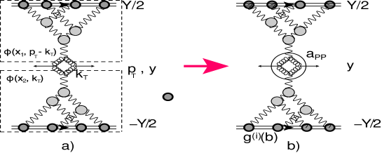
Refer to caption
Figure 24: The graphic representation of Eq. (83) (see Fig. 24-a).For the sake of simplicity all other indices in ϕ(x1,pTkT)italic-ϕsubscript𝑥1subscript𝑝𝑇subscript𝑘𝑇\phi\left(x_{1},p_{T}-k_{T}\right) and ϕ(x2,kT)italic-ϕsubscript𝑥2subscript𝑘𝑇\phi\left(x_{2},k_{T}\right) are omitted. The wavy lines denote the BFKL Pomerons, while the helical lines illustrate the gluons. In Fig. 24-b the Mueller diagram for inclusive production is shown.

In our model the sum of ‘fan’ diagrams is given by Eq. (29). Assuming that the main contribution to

dσdy=d2pTdσdyd2pT𝑑𝜎𝑑𝑦superscript𝑑2subscript𝑝𝑇𝑑𝜎𝑑𝑦superscript𝑑2subscript𝑝𝑇\frac{d\sigma}{dy}\,=\,\int d^{2}p_{T}\,\frac{d\sigma}{dy\,d^{2}p_{T}}

stems from pTQssubscript𝑝𝑇subscript𝑄𝑠p_{T}\,\leq\,Q_{s}, we obtain the following formula:

dσdy𝑑𝜎𝑑𝑦\displaystyle\frac{d\sigma}{dy}\,\, =\displaystyle= d2pTdσdyd2pT=aIPIPln(W/W0)(α2In(1)(12Y+y)+β2In(2)(12Y+y))superscript𝑑2subscript𝑝𝑇𝑑𝜎𝑑𝑦superscript𝑑2subscript𝑝𝑇subscript𝑎𝐼𝑃𝐼𝑃𝑊subscript𝑊0superscript𝛼2𝐼superscript𝑛112𝑌𝑦superscript𝛽2𝐼superscript𝑛212𝑌𝑦\displaystyle\,\,\int d^{2}p_{T}\,\frac{d\sigma}{dy\,d^{2}p_{T}}\,\,=\,\,a_{{I\!\!P}{I\!\!P}}\,\ln\left(W/W_{0}\right)\Bigg{(}\alpha^{2}\,In^{(1)}\left(\frac{1}{2}Y+y\right)\,+\beta^{2}\,In^{(2)}\left(\frac{1}{2}Y+y\right)\Bigg{)} (84)
×\displaystyle\times (α2In(1)(12Yy)+β2In(2)(12Yy))superscript𝛼2𝐼superscript𝑛112𝑌𝑦superscript𝛽2𝐼superscript𝑛212𝑌𝑦\displaystyle\Bigg{(}\alpha^{2}\,In^{(1)}\left(\frac{1}{2}Y-y\right)\,+\beta^{2}\,In^{(2)}\left(\frac{1}{2}Y-y\right)\Bigg{)}

where

In(i)(y)=d2bNBK(g(i)S(mi,b)G~IP(y))orIn(i)(y)=IiBK(y,QT=0);formulae-sequence𝐼superscript𝑛𝑖𝑦superscript𝑑2𝑏superscript𝑁𝐵𝐾superscript𝑔𝑖𝑆subscript𝑚𝑖𝑏subscript~𝐺𝐼𝑃𝑦or𝐼superscript𝑛𝑖𝑦subscriptsuperscript𝐼BK𝑖𝑦subscript𝑄𝑇0\displaystyle In^{(i)}\left(y\right)\,=\,\int d^{2}b\,\,N^{BK}\left(g^{(i)}\,S\left(m_{i},b\right)\,\tilde{G}_{I\!\!P}\left(y\right)\right)~{}~{}~{}~{}~{}~{}~{}\mbox{or}~{}~{}~{}~{}~{}~{}In^{(i)}\left(y\right)=I^{\rm BK}_{i}\left(y,Q_{T}=0\right);
withIiBK(y,QT)=d2bei𝒃𝑸TNBK(g(i)S(mi,b)G~IP(y))withsubscriptsuperscript𝐼BK𝑖𝑦subscript𝑄𝑇superscript𝑑2𝑏superscript𝑒𝑖𝒃subscript𝑸𝑇superscript𝑁𝐵𝐾superscript𝑔𝑖𝑆subscript𝑚𝑖𝑏subscript~𝐺𝐼𝑃𝑦\displaystyle~{}~{}~{}\mbox{with}~{}~{}~{}I^{\rm BK}_{i}\left(y,Q_{T}\right)\,=\,\int d^{2}b\,e^{i\boldsymbol{b}\cdot\boldsymbol{Q}_{T}}\,\,N^{BK}\left(g^{(i)}\,S\left(m_{i},b\right)\,\tilde{G}_{I\!\!P}\left(y\right)\right) (85)

where G~IP(y)subscript~𝐺𝐼𝑃𝑦\tilde{G}_{I\!\!P}\left(y\right) and NBKsuperscript𝑁𝐵𝐾N^{BK} have been defined in Eq. (46) and in Eq. (29), respectively. Regarding the factor in front of Eq. (84) i.e. ln(W/W0)𝑊subscript𝑊0\ln\left(W/W_{0}\right), where W=s𝑊𝑠W=\sqrt{s} is the energy of collision in c.m. frame, and W0subscript𝑊0W_{0} is the value of energy from which we start our approach. One can see that Eq. (83) is divergent in the region of small pT<Qssubscript𝑝𝑇subscript𝑄𝑠p_{T}\,<\,Q_{s}. Indeed, in this region ϕitalic-ϕ\phi’s in Eq. (83) do not depend on pTsubscript𝑝𝑇p_{T}, since kTQs>pTsubscript𝑘𝑇subscript𝑄𝑠subscript𝑝𝑇k_{T}\approx\,Q_{s}\,>\,p_{T}, and the integration over pTsubscript𝑝𝑇p_{T} leads to ln(Qs2/msoft2)subscriptsuperscript𝑄2𝑠subscriptsuperscript𝑚2𝑠𝑜𝑓𝑡\ln\left(Q^{2}_{s}/m^{2}_{soft}\right), where msoftsubscript𝑚𝑠𝑜𝑓𝑡m_{soft} is the non-perturbative scale, that includes the confinement of quarks and gluons (msoftΛQCD)m_{soft}\sim\Lambda_{QCD}).

B.0.2 LRR correlations

In our previous paper GLMCOR , we showed that in the framework of our model that has been described above, the main source of the long range rapidity correlation, is the correlation between two parton showers. In other words, it was shown that the contribution to the correlation function from enhanced and semi-enhanced diagrams, turns out to be negligibly small.

The appropriate Mueller diagrams are shown in Fig. 25. Examining this diagram, we see that the contribution to the double inclusive cross section, differs from the product of two single inclusive cross sections. This difference generates the rapidity correlation function, which is defined as

R(y1,y2)=1σind2σdy1dy21σindσdy11σindσdy2  1𝑅subscript𝑦1subscript𝑦21subscript𝜎𝑖𝑛superscript𝑑2𝜎𝑑subscript𝑦1𝑑subscript𝑦21subscript𝜎𝑖𝑛𝑑𝜎𝑑subscript𝑦11subscript𝜎𝑖𝑛𝑑𝜎𝑑subscript𝑦21R\left(y_{1},y_{2}\right)\,\,=\,\ \frac{\frac{1}{\sigma_{in}}\frac{d^{2}\sigma}{dy_{1}\,dy_{2}}}{\frac{1}{\sigma_{in}}\frac{d\sigma}{dy_{1}}\,\frac{1}{\sigma_{in}}\frac{d\sigma}{dy_{2}}}\,\,-\,\,1 (86)
Refer to caption
Figure 25: The Mueller diagram for the rapidity correlation between two particles produced in two parton showers. Fig. 25-a shows the first Mueller diagram, while Fig. 25-b indicates the structure of general diagrams. The double wavy lines describe the dressed BFKL Pomerons. The blobs stand for the vertices as shown in the legend.

There are two reasons for the difference between the double inclusive cross section due to production of two parton showers, and the products of inclusive cross sections: the first, is that in the expression for the double inclusive cross section, we integrate the product of the single inclusive inclusive cross sections, over b𝑏b or QTsubscript𝑄𝑇Q_{T}(see Fig. 24-a and Eq. (13)). The second, is that the summation over i𝑖i and k𝑘k for the product of single inclusive cross sections, is for fixed i𝑖i and k𝑘k(see Fig. 24-a).

Introducing the following new function, enables us to write the analytical expression for the double inclusive cross section:

I(i,k)(y,b)superscript𝐼𝑖𝑘𝑦𝑏\displaystyle I^{(i,k)}\left(y,b\right)\,\, =\displaystyle= a~IPIPd2bNBK(g(i)S(mi,b)G~dressed(r=1/m,12Y+y))subscript~𝑎𝐼𝑃𝐼𝑃superscript𝑑2superscript𝑏superscript𝑁𝐵𝐾superscript𝑔𝑖𝑆subscript𝑚𝑖superscript𝑏superscript~𝐺dressedsubscript𝑟bottom1𝑚12𝑌𝑦\displaystyle\,\,\tilde{a}_{{I\!\!P}{I\!\!P}}\,\int d^{2}b^{\prime}\,\,N^{BK}\Bigg{(}g^{(i)}\,S\left(m_{i},b^{\prime}\right)\tilde{G}^{\mbox{\tiny dressed}}\left(r_{\bot}=1/m,\frac{1}{2}Y+y\right)\Bigg{)}\, (87)
×\displaystyle\times NBK(g(k)S(mk,𝒃𝒃)G~dressed(r=1/m,12Yy))superscript𝑁𝐵𝐾superscript𝑔𝑘𝑆subscript𝑚𝑘𝒃superscript𝒃superscript~𝐺dressedsubscript𝑟bottom1𝑚12𝑌𝑦\displaystyle N^{BK}\Bigg{(}g^{(k)}\,S\left(m_{k},\boldsymbol{b}-\boldsymbol{b}^{\,{}^{\prime}}\right)\tilde{G}^{\mbox{\tiny dressed}}\left(r_{\bot}=1/m,\frac{1}{2}Y-y\right)\Bigg{)}

where a~IPIP=aIPIPln(W/W0)subscript~𝑎𝐼𝑃𝐼𝑃subscript𝑎𝐼𝑃𝐼𝑃𝑊subscript𝑊0\tilde{a}_{{I\!\!P}{I\!\!P}}=a_{{I\!\!P}{I\!\!P}}\,\ln\left(W/W_{0}\right).

Using Eq. (87) we can write the double inclusive cross section in two equivalent forms

d2σ2 parton showersdy1dy2=d2p1Td2p2Td2σ2 parton showersdy1dy2d2p1Td2p2T=d2b{α4I(1,1)(y1,b)I(1,1)(y2,b)\displaystyle\frac{d^{2}\sigma^{\mbox{\tiny 2 parton showers}}}{dy_{1}\,\,dy_{2}}\,\,=\,\,\int d^{2}p_{1T}\,d^{2}p_{2T}\frac{d^{2}\sigma^{\mbox{\tiny 2 parton showers}}}{dy_{1}\,\,dy_{2}\,d^{2}p_{1T}\,d^{2}p_{2T}}\,\,=\,\,\int d^{2}b\,\,\Bigg{\{}\alpha^{4}\,I^{(1,1)}\left(y_{1},b\right)\,I^{(1,1)}\left(y_{2},b\right)
+α2β2(I(1,2)(y1,b)I(1,2)(y2,b)+I(2,1)(y1,b)I(2,1)(y2,b))+β4I(2,2)(y1,b)I(2,2)(y2,b)}\displaystyle+\alpha^{2}\,\beta^{2}\,\left(I^{(1,2)}\left(y_{1},b\right)\,I^{(1,2)}\left(y_{2},b\right)\,\,+\,\,I^{(2,1)}\left(y_{1},b\right)\,I^{(2,1)}\left(y_{2},b\right)\right)\,\,+\,\,\beta^{4}\,I^{(2,2)}\left(y_{1},b\right)\,I^{(2,2)}\left(y_{2},b\right)\Bigg{\}} (88)
=a~IPIP2pT12pT22d2QT(α2I1BK(12Y+y1;QT)I1BK(12Y+y2;QT)+β2I2BK(12Y+y1;QT)I2BK(12Y+y2;QT))absentsubscriptsuperscript~𝑎2𝐼𝑃𝐼𝑃subscriptsuperscript𝑝2𝑇1subscriptsuperscript𝑝2𝑇2superscript𝑑2subscript𝑄𝑇superscript𝛼2subscriptsuperscript𝐼BK112𝑌subscript𝑦1subscript𝑄𝑇subscriptsuperscript𝐼BK112𝑌subscript𝑦2subscript𝑄𝑇superscript𝛽2subscriptsuperscript𝐼BK212𝑌subscript𝑦1subscript𝑄𝑇subscriptsuperscript𝐼BK212𝑌subscript𝑦2subscript𝑄𝑇\displaystyle=\frac{\tilde{a}^{2}_{{I\!\!P}{I\!\!P}}}{p^{2}_{T1}\,p^{2}_{T2}}\,\int d^{2}Q_{T}\Bigg{(}\alpha^{2}I^{\rm BK}_{1}\left(\frac{1}{2}Y+y_{1};Q_{T}\right)I^{\rm BK}_{1}\left(\frac{1}{2}Y+y_{2};Q_{T}\right)\,+\,\beta^{2}\,I^{\rm BK}_{2}\left(\frac{1}{2}Y+y_{1};Q_{T}\right)I^{\rm BK}_{2}\left(\frac{1}{2}Y+y_{2};Q_{T}\right)\Bigg{)}
×(α2I1BK(12Yy1;QT)I1BK(12Yy2;QT)+β2I2BK(12Yy1;QT)I2BK(12Yy2;QT))absentsuperscript𝛼2subscriptsuperscript𝐼BK112𝑌subscript𝑦1subscript𝑄𝑇subscriptsuperscript𝐼BK112𝑌subscript𝑦2subscript𝑄𝑇superscript𝛽2subscriptsuperscript𝐼BK212𝑌subscript𝑦1subscript𝑄𝑇subscriptsuperscript𝐼BK212𝑌subscript𝑦2subscript𝑄𝑇\displaystyle\times\,\Bigg{(}\alpha^{2}I^{\rm BK}_{1}\left(\frac{1}{2}Y-y_{1};Q_{T}\right)I^{\rm BK}_{1}\left(\frac{1}{2}Y-y_{2};Q_{T}\right)\,+\,\beta^{2}\,I^{\rm BK}_{2}\left(\frac{1}{2}Y-y_{1};Q_{T}\right)I^{\rm BK}_{2}\left(\frac{1}{2}Y-y_{2};Q_{T}\right)\Bigg{)}\,
a~IPIP2pT12pT22d2QTF12BK(12Y+y1,12Y+y2;QT)F12BK(12Yy1,12Yy2;QT)absentsubscriptsuperscript~𝑎2𝐼𝑃𝐼𝑃subscriptsuperscript𝑝2𝑇1subscriptsuperscript𝑝2𝑇2superscript𝑑2subscript𝑄𝑇subscriptsuperscript𝐹BK1212𝑌subscript𝑦112𝑌subscript𝑦2subscript𝑄𝑇subscriptsuperscript𝐹BK1212𝑌subscript𝑦112𝑌subscript𝑦2subscript𝑄𝑇\displaystyle\equiv\,\,\,\frac{\tilde{a}^{2}_{{I\!\!P}{I\!\!P}}}{p^{2}_{T1}\,p^{2}_{T2}}\,\int d^{2}Q_{T}\,F^{\rm BK}_{12}\left(\frac{1}{2}Y+y_{1},\frac{1}{2}Y+y_{2};Q_{T}\right)\,\,F^{\rm BK}_{12}\left(\frac{1}{2}Y-y_{1},\frac{1}{2}Y-y_{2};Q_{T}\right) (89)

where F12BKsubscriptsuperscript𝐹BK12F^{\rm BK}_{12} is equal to

F12BK(Y1,Y2;QT)=α2I1BK(Y1;QT)I1BK(Y2;QT)+β2I2BK(Y1;QT)I2BK(Y2;QT)subscriptsuperscript𝐹BK12subscript𝑌1subscript𝑌2subscript𝑄𝑇superscript𝛼2subscriptsuperscript𝐼BK1subscript𝑌1subscript𝑄𝑇subscriptsuperscript𝐼BK1subscript𝑌2subscript𝑄𝑇superscript𝛽2subscriptsuperscript𝐼BK2subscript𝑌1subscript𝑄𝑇subscriptsuperscript𝐼BK2subscript𝑌2subscript𝑄𝑇F^{\rm BK}_{12}\left(Y_{1},Y_{2};Q_{T}\right)\,=\,\alpha^{2}I^{\rm BK}_{1}\left(Y_{1};Q_{T}\right)I^{\rm BK}_{1}\left(Y_{2};Q_{T}\right)\,+\,\beta^{2}\,I^{\rm BK}_{2}\left(Y_{1};Q_{T}\right)I^{\rm BK}_{2}\left(Y_{2};Q_{T}\right) (90)

Recall that all rapidities are in the c.m. frame.

B.0.3 𝒗𝒏subscript𝒗𝒏v_{n} for proton-proton collisions

Using Eq. (89), Eq. (10) can be re-written in the following form

d2σdy1dy2d2pT1d2pT2=a~IPIP2pT12pT22d2kTF12BK(12Y+y1,12Y+y2;kT)F12BK(12Yy1,12Yy2;kT)superscript𝑑2𝜎𝑑subscript𝑦1𝑑subscript𝑦2superscript𝑑2subscript𝑝𝑇1superscript𝑑2subscript𝑝𝑇2subscriptsuperscript~𝑎2𝐼𝑃𝐼𝑃subscriptsuperscript𝑝2𝑇1subscriptsuperscript𝑝2𝑇2superscript𝑑2subscript𝑘𝑇subscriptsuperscript𝐹BK1212𝑌subscript𝑦112𝑌subscript𝑦2subscript𝑘𝑇subscriptsuperscript𝐹BK1212𝑌subscript𝑦112𝑌subscript𝑦2subscript𝑘𝑇\displaystyle\frac{d^{2}\sigma}{dy_{1}\,dy_{2}d^{2}p_{T1}d^{2}p_{T2}}\,\,=\,\,\frac{\tilde{a}^{2}_{{I\!\!P}{I\!\!P}}}{p^{2}_{T1}\,p^{2}_{T2}}\,\int d^{2}k_{T}\,F^{\rm BK}_{12}\left(\frac{1}{2}Y+y_{1},\frac{1}{2}Y+y_{2};k_{T}\right)\,\,F^{\rm BK}_{12}\left(\frac{1}{2}Y-y_{1},\frac{1}{2}Y-y_{2};k_{T}\right) (91)
+a~IPIP2Nc2114(1pT12+1pT22)2d2kTF12BK(12Y+y1,12Y+y2;𝒌T)F12BK(12Yy1,12Yy2;𝒌T+𝒑T,12)subscriptsuperscript~𝑎2𝐼𝑃𝐼𝑃subscriptsuperscript𝑁2𝑐114superscript1subscriptsuperscript𝑝2𝑇11subscriptsuperscript𝑝2𝑇22superscript𝑑2subscript𝑘𝑇subscriptsuperscript𝐹BK1212𝑌subscript𝑦112𝑌subscript𝑦2subscript𝒌𝑇subscriptsuperscript𝐹BK1212𝑌subscript𝑦112𝑌subscript𝑦2subscript𝒌𝑇subscript𝒑𝑇12\displaystyle+\,\,\frac{\tilde{a}^{2}_{{I\!\!P}{I\!\!P}}}{N^{2}_{c}-1}\,\frac{1}{4}\left(\frac{1}{p^{2}_{T1}}\,+\,\frac{1}{p^{2}_{T2}}\right)^{2}\int d^{2}k_{T}\,F^{\rm BK}_{12}\left(\frac{1}{2}Y+y_{1},\frac{1}{2}Y+y_{2};\boldsymbol{k}_{T}\right)\,\,F^{\rm BK}_{12}\left(\frac{1}{2}Y-y_{1},\frac{1}{2}Y-y_{2};\boldsymbol{k}_{T}+\boldsymbol{p}_{T,12}\right)

In Eq. (91) we neglected the contribution pT,122proportional-toabsentsubscriptsuperscript𝑝2𝑇12\propto p^{2}_{T,12} in the vertex of gluon emission in Fig. 22 (see Appendix A1), as well as the dependence of the BFKL Pomeron on the momentum transfer. The small size of both quantities stem from the fact that in our model, kTsubscript𝑘𝑇k_{T} dependence in Eq. (91) is determined by the proton structure and the typical kTm1similar-tosubscript𝑘𝑇subscript𝑚1k_{T}\sim m_{1}{\rm} or m2subscript𝑚2m_{2} (see Table 1), while typical transverse momentum in the BFKL Pomeron is about Qssubscript𝑄𝑠Q_{s} or m𝑚m, and it is much larger than m1subscript𝑚1m_{1} or m2subscript𝑚2m_{2}.

Appendix C Hadron-nucleus interaction in the model

In the case of the hadron-nucleus interaction the general formula of Eq. (89) can be re-written in the formGLMPA

d2σ2 parton showersdy1dy2=d2p1Td2p2Td2σ2 parton showersdy1dy2d2p1Td2p2T=superscript𝑑2superscript𝜎2 parton showers𝑑subscript𝑦1𝑑subscript𝑦2superscript𝑑2subscript𝑝1𝑇superscript𝑑2subscript𝑝2𝑇superscript𝑑2superscript𝜎2 parton showers𝑑subscript𝑦1𝑑subscript𝑦2superscript𝑑2subscript𝑝1𝑇superscript𝑑2subscript𝑝2𝑇absent\displaystyle\frac{d^{2}\sigma^{\mbox{\tiny 2 parton showers}}}{dy_{1}\,\,dy_{2}}\,\,=\,\,\int d^{2}p_{1T}\,d^{2}p_{2T}\frac{d^{2}\sigma^{\mbox{\tiny 2 parton showers}}}{dy_{1}\,\,dy_{2}\,d^{2}p_{1T}\,d^{2}p_{2T}}\,\,= (92)
=a~IPIP2pT12pT22d2QT(α2I1BK(12Y+y1;QT)I1BK(12Y+y2;QT)+β2I2BK(12Y+y1;QT)I2BK(12Y+y2;QT))absentsubscriptsuperscript~𝑎2𝐼𝑃𝐼𝑃subscriptsuperscript𝑝2𝑇1subscriptsuperscript𝑝2𝑇2superscript𝑑2subscript𝑄𝑇superscript𝛼2subscriptsuperscript𝐼BK112𝑌subscript𝑦1subscript𝑄𝑇subscriptsuperscript𝐼BK112𝑌subscript𝑦2subscript𝑄𝑇superscript𝛽2subscriptsuperscript𝐼BK212𝑌subscript𝑦1subscript𝑄𝑇subscriptsuperscript𝐼BK212𝑌subscript𝑦2subscript𝑄𝑇\displaystyle=\frac{\tilde{a}^{2}_{{I\!\!P}{I\!\!P}}}{p^{2}_{T1}\,p^{2}_{T2}}\,\int d^{2}Q_{T}\Bigg{(}\alpha^{2}I^{\rm BK}_{1}\left(\frac{1}{2}Y+y_{1};Q_{T}\right)I^{\rm BK}_{1}\left(\frac{1}{2}Y+y_{2};Q_{T}\right)\,+\,\beta^{2}\,I^{\rm BK}_{2}\left(\frac{1}{2}Y+y_{1};Q_{T}\right)I^{\rm BK}_{2}\left(\frac{1}{2}Y+y_{2};Q_{T}\right)\Bigg{)}
×IABK(12Yy1;QT)IABK(12Yy2;QT)absentsubscriptsuperscript𝐼BK𝐴12𝑌subscript𝑦1subscript𝑄𝑇subscriptsuperscript𝐼BK𝐴12𝑌subscript𝑦2subscript𝑄𝑇\displaystyle\times\,I^{\rm BK}_{A}\left(\frac{1}{2}Y-y_{1};Q_{T}\right)\,I^{\rm BK}_{A}\left(\frac{1}{2}Y-y_{2};Q_{T}\right)\ \,
a~IPIP2pT12pT22d2QTF12BK(12Y+y1,12Y+y2;QT)FABK(12Yy1,12Yy2;QT)absentsubscriptsuperscript~𝑎2𝐼𝑃𝐼𝑃subscriptsuperscript𝑝2𝑇1subscriptsuperscript𝑝2𝑇2superscript𝑑2subscript𝑄𝑇subscriptsuperscript𝐹BK1212𝑌subscript𝑦112𝑌subscript𝑦2subscript𝑄𝑇subscriptsuperscript𝐹BK𝐴12𝑌subscript𝑦112𝑌subscript𝑦2subscript𝑄𝑇\displaystyle\equiv\,\,\,\frac{\tilde{a}^{2}_{{I\!\!P}{I\!\!P}}}{p^{2}_{T1}\,p^{2}_{T2}}\,\int d^{2}Q_{T}\,F^{\rm BK}_{12}\left(\frac{1}{2}Y+y_{1},\frac{1}{2}Y+y_{2};Q_{T}\right)\,\,F^{\rm BK}_{A}\left(\frac{1}{2}Y-y_{1},\frac{1}{2}Y-y_{2};Q_{T}\right) (93)

where

IABK(y,QT)=d2bei𝒃𝑸TNBK((α2In(1)(y)+β2In(2)(y))SA(b))subscriptsuperscript𝐼BK𝐴𝑦subscript𝑄𝑇superscript𝑑2𝑏superscript𝑒𝑖𝒃subscript𝑸𝑇superscript𝑁BKsuperscript𝛼2𝐼superscript𝑛1𝑦superscript𝛽2𝐼superscript𝑛2𝑦subscript𝑆𝐴𝑏I^{\rm BK}_{A}\left(y,Q_{T}\right)\,\,=\,\,\int d^{2}be^{i\boldsymbol{b}\cdot\boldsymbol{Q}_{T}}\,N^{\rm BK}\left(\left(\alpha^{2}In^{(1)}\left(y\right)\,+\,\beta^{2}\,In^{(2)}\left(y\right)\right)S_{A}\left(b\right)\right) (94)

where In(i)𝐼superscript𝑛𝑖In^{(i)} are defined in Eq. (B.0.1) and SA(b)subscript𝑆𝐴𝑏S_{A}\left(b\right) is the nucleus Wood-Saxon distributionWS given by

SA(b)=𝑑zρ01+exp(z2+b2RAh)whered2bSA(b)=Aformulae-sequencesubscript𝑆𝐴𝑏subscriptsuperscriptdifferential-d𝑧subscript𝜌01superscript𝑧2superscript𝑏2subscript𝑅𝐴wheresuperscript𝑑2𝑏subscript𝑆𝐴𝑏𝐴S_{A}\left(b\right)\,\,=\,\ \int^{\infty}_{-\infty}dz\,\frac{\rho_{0}}{1\,+\,\exp\Big{(}\frac{\sqrt{z^{2}+b^{2}}-R_{A}}{h}\Big{)}}~{}~{}~{}~{}~{}~{}~{}~{}\mbox{where}~{}~{}~{}~{}~{}~{}\int d^{2}b\,S_{A}\left(b\right)\,=\,A (95)

For gold we have RA=6.38fmsubscript𝑅𝐴6.38𝑓𝑚R_{A}=6.38\,fm and h=0.535fm0.535𝑓𝑚h=0.535\,fm, while for lead we have RA=6.68fmsubscript𝑅𝐴6.68𝑓𝑚R_{A}=6.68\,fm and h=0.546fm0.546𝑓𝑚h=0.546\,fm WS . In Eq. (93) we have taken into account that the typical impact parameters in hadron-hadron interaction are much smaller than the radius of nucleus (RAsubscript𝑅𝐴R_{A}). Indeed, the typical b𝑏b in hadron-hadron collisions are αeffYsubscriptsuperscript𝛼𝑒𝑓𝑓𝑌\alpha^{\prime}_{eff}Y or less, where αeffsubscriptsuperscript𝛼𝑒𝑓𝑓\alpha^{\prime}_{eff} is the effective slope of the BFKL Pomeron trajectory, which occurs in our model as a result of shadowing corrections.

Using Eq. (93) we can re-write Eq. (91) for proton-proton in the following form for proton-nucleus scattering

d2σdy1dy2d2pT1d2pT2=a~IPIP2pT12pT22d2kTF12BK(12Y+y1,12Y+y2;kT)FABK(12Yy1,12Yy2;kT)superscript𝑑2𝜎𝑑subscript𝑦1𝑑subscript𝑦2superscript𝑑2subscript𝑝𝑇1superscript𝑑2subscript𝑝𝑇2subscriptsuperscript~𝑎2𝐼𝑃𝐼𝑃subscriptsuperscript𝑝2𝑇1subscriptsuperscript𝑝2𝑇2superscript𝑑2subscript𝑘𝑇subscriptsuperscript𝐹BK1212𝑌subscript𝑦112𝑌subscript𝑦2subscript𝑘𝑇subscriptsuperscript𝐹BK𝐴12𝑌subscript𝑦112𝑌subscript𝑦2subscript𝑘𝑇\displaystyle\frac{d^{2}\sigma}{dy_{1}\,dy_{2}d^{2}p_{T1}d^{2}p_{T2}}\,\,=\,\,\frac{\tilde{a}^{2}_{{I\!\!P}{I\!\!P}}}{p^{2}_{T1}\,p^{2}_{T2}}\,\int d^{2}k_{T}\,F^{\rm BK}_{12}\left(\frac{1}{2}Y+y_{1},\frac{1}{2}Y+y_{2};k_{T}\right)\,\,F^{\rm BK}_{A}\left(\frac{1}{2}Y-y_{1},\frac{1}{2}Y-y_{2};k_{T}\right) (96)
+a~IPIP2Nc2114(1pT12+1pT22)2d2kTF12BK(12Y+y1,12Y+y2;𝒌T+𝒑T,12)FABK(12Yy1,12Yy2;𝒌T)subscriptsuperscript~𝑎2𝐼𝑃𝐼𝑃subscriptsuperscript𝑁2𝑐114superscript1subscriptsuperscript𝑝2𝑇11subscriptsuperscript𝑝2𝑇22superscript𝑑2subscript𝑘𝑇subscriptsuperscript𝐹BK1212𝑌subscript𝑦112𝑌subscript𝑦2subscript𝒌𝑇subscript𝒑𝑇12subscriptsuperscript𝐹BK𝐴12𝑌subscript𝑦112𝑌subscript𝑦2subscript𝒌𝑇\displaystyle+\,\,\frac{\tilde{a}^{2}_{{I\!\!P}{I\!\!P}}}{N^{2}_{c}-1}\,\frac{1}{4}\left(\frac{1}{p^{2}_{T1}}\,+\,\frac{1}{p^{2}_{T2}}\right)^{2}\int d^{2}k_{T}\,F^{\rm BK}_{12}\left(\frac{1}{2}Y+y_{1},\frac{1}{2}Y+y_{2};\boldsymbol{k}_{T}+\boldsymbol{p}_{T,12}\right)\,\,F^{\rm BK}_{A}\left(\frac{1}{2}Y-y_{1},\frac{1}{2}Y-y_{2};\boldsymbol{k}_{T}\right)

and for nucleus-nuclues scattering we have

d2σdy1dy2d2pT1d2pT2=a~IPIP2pT12pT22d2kTF12BK(12Y+y1,12Y+y2;kT)FABK(12Yy1,12Yy2;kT)superscript𝑑2𝜎𝑑subscript𝑦1𝑑subscript𝑦2superscript𝑑2subscript𝑝𝑇1superscript𝑑2subscript𝑝𝑇2subscriptsuperscript~𝑎2𝐼𝑃𝐼𝑃subscriptsuperscript𝑝2𝑇1subscriptsuperscript𝑝2𝑇2superscript𝑑2subscript𝑘𝑇subscriptsuperscript𝐹BK1212𝑌subscript𝑦112𝑌subscript𝑦2subscript𝑘𝑇subscriptsuperscript𝐹BK𝐴12𝑌subscript𝑦112𝑌subscript𝑦2subscript𝑘𝑇\displaystyle\frac{d^{2}\sigma}{dy_{1}\,dy_{2}d^{2}p_{T1}d^{2}p_{T2}}\,\,=\,\,\frac{\tilde{a}^{2}_{{I\!\!P}{I\!\!P}}}{p^{2}_{T1}\,p^{2}_{T2}}\,\int d^{2}k_{T}\,F^{\rm BK}_{12}\left(\frac{1}{2}Y+y_{1},\frac{1}{2}Y+y_{2};k_{T}\right)\,\,F^{\rm BK}_{A}\left(\frac{1}{2}Y-y_{1},\frac{1}{2}Y-y_{2};k_{T}\right) (97)
+a~IPIP2Nc2114(1pT12+1pT22)2d2kTFABK(12Y+y1,12Y+y2;𝒌T+𝒑T,12)FABK(12Yy1,12Yy2;𝒌T)subscriptsuperscript~𝑎2𝐼𝑃𝐼𝑃subscriptsuperscript𝑁2𝑐114superscript1subscriptsuperscript𝑝2𝑇11subscriptsuperscript𝑝2𝑇22superscript𝑑2subscript𝑘𝑇subscriptsuperscript𝐹BK𝐴12𝑌subscript𝑦112𝑌subscript𝑦2subscript𝒌𝑇subscript𝒑𝑇12subscriptsuperscript𝐹BK𝐴12𝑌subscript𝑦112𝑌subscript𝑦2subscript𝒌𝑇\displaystyle+\,\,\frac{\tilde{a}^{2}_{{I\!\!P}{I\!\!P}}}{N^{2}_{c}-1}\,\frac{1}{4}\left(\frac{1}{p^{2}_{T1}}\,+\,\frac{1}{p^{2}_{T2}}\right)^{2}\int d^{2}k_{T}\,F^{\rm BK}_{A}\left(\frac{1}{2}Y+y_{1},\frac{1}{2}Y+y_{2};\boldsymbol{k}_{T}+\boldsymbol{p}_{T,12}\right)\,\,F^{\rm BK}_{A}\left(\frac{1}{2}Y-y_{1},\frac{1}{2}Y-y_{2};\boldsymbol{k}_{T}\right)

References

  • (1) E. Gotsman, E. Levin and U. Maor, arXiv:1604.04461 [hep-ph].
  • (2) V. Khachatryan et al. [CMS Collaboration], arXiv:1510.03068 [nucl-ex];  JHEP 1009 (2010) 091 [arXiv:1009.4122 [hep-ex]]. arXiv:1510.03068 [nucl-ex].
  • (3) J. Adams et al. [STAR Collaboration], Phys. Rev. Lett.  95 (2005) 152301 [nucl-ex/0501016].
  • (4) B. Alver et al. [PHOBOS Collaboration], Phys. Rev. Lett.  104 (2010) 062301 [arXiv:0903.2811 [nucl-ex]].
  • (5) H. Agakishiev et al. [STAR Collaboration], arXiv:1010.0690 [nucl-ex].
  • (6) S. Chatrchyan et al. [CMS Collaboration], Phys. Lett. B 718 (2013) 795 [arXiv:1210.5482 [nucl-ex]];    V. Khachatryan et al. [CMS Collaboration], JHEP 1009 (2010) 091, [arXiv:1009.4122 [hep-ex]].
  • (7) S. Chatrchyan et al. [CMS Collaboration], JHEP 1402 (2014) 088, [arXiv:1312.1845 [nucl-ex]];  Phys. Rev. C 89 (2014) no.4, 044906;  [arXiv:1310.8651 [nucl-ex]];  “Centrality dependence of dihadron correlations and azimuthal anisotropy harmonics in PbPb collisions at sNN=2.76subscript𝑠𝑁𝑁2.76\sqrt{s_{NN}}=2.76 TeV,” Eur. Phys. J. C 72 (2012) 2012 [arXiv:1201.3158 [nucl-ex]];    JHEP 1402 (2014) 088 doi:10.1007/JHEP02(2014)088 [arXiv:1312.1845 [nucl-ex]].
  • (8) J. Adam et al. [ALICE Collaboration], arXiv:1604.07663 [nucl-ex];    Phys. Rev. Lett.  116 (2016) no.13, 132302 doi:10.1103/PhysRevLett.116.132302 [arXiv:1602.01119 [nucl-ex]];    L. Milano [ALICE Collaboration], Nucl. Phys. A 931 (2014) 1017, [arXiv:1407.5808 [hep-ex]];   Y. Zhou [ALICE Collaboration], J. Phys. Conf. Ser.  509 (2014) 012029, [arXiv:1309.3237 [nucl-ex]].   
  • (9) B. B. Abelev et al. [ALICE Collaboration], Phys. Rev. C 90 (2014) no.5, 054901, [arXiv:1406.2474 [nucl-ex]];    B. B. Abelev et al. [ALICE Collaboration], Phys. Lett. B 726 (2013) 164 doi:10.1016/j.physletb.2013.08.024 [arXiv:1307.3237 [nucl-ex]];   B. Abelev et al. [ALICE Collaboration], Phys. Lett. B 719 (2013) 29, [arXiv:1212.2001 [nucl-ex]].
  • (10) G. Aad et al. [ATLAS Collaboration], Phys. Rev. Lett.  116 (2016) 172301, [arXiv:1509.04776 [hep-ex]].
  • (11) G. Aad et al. [ATLAS Collaboration], Phys. Rev. C 90 (2014) no.4, 044906;  [arXiv:1409.1792 [hep-ex]];    B. Wosiek [ATLAS Collaboration], Annals Phys.  352 (2015) 117;   G. Aad et al. [ATLAS Collaboration], Phys. Lett. B 725 (2013) 60, [arXiv:1303.2084 [hep-ex]]. 
  • (12) B. Wosiek [ATLAS Collaboration], Phys. Rev. C 86 (2012) 014907, [arXiv:1203.3087 [hep-ex]].  
  • (13) E. M. Levin, M. G. Ryskin and S. I. Troian, Sov. J. Nucl. Phys.  23 (1976) 222 [Yad. Fiz.  23 (1976) 423];     A. Capella, A. Krzywicki and E. M. Levin, Phys. Rev. D 44 (1991) 704.
  • (14) Y. V. Kovchegov and D. E. Wertepny, Nucl. Phys. A 906 (2013) 50, [arXiv:1212.1195 [hep-ph]];   
  • (15) T. Altinoluk, N. Armesto, G. Beuf, A. Kovner and M. Lublinsky, Phys. Lett. B 752 (2016) 113, [arXiv:1509.03223 [hep-ph]];    T. Altinoluk, N. Armesto, G. Beuf, A. Kovner and M. Lublinsky, Phys. Lett. B 751 (2015) 448, [arXiv:1503.07126 [hep-ph]].
  • (16) Yuri V Kovchegov and Eugene Levin, “ Quantum Choromodynamics at High Energies", Cambridge Monographs on Particle Physics, Nuclear Physics and Cosmology, Cambridge University Press, 2012 .
  • (17) R. Hanbury Brown and R. Q. Twiss, Nature 178 (1956) 1046.
  • (18) G. Goldhaber, W. B. Fowler, S. Goldhaber and T. F. Hoang, Phys. Rev. Lett.  3, 181 (1959);    G. I. Kopylov and M. I. Podgoretsky, Sov. J. Nucl. Phys.  15, 219 (1972) [Yad. Fiz.  15, 392 (1972)];    G. Alexander, Rept. Prog. Phys.  66 (2003) 481, [hep-ph/0302130].
  • (19) A. H. Mueller, Phys. Rev. D2 (1970) 2963.
  • (20) E. A. Kuraev, L. N. Lipatov, and F. S. Fadin, Sov. Phys. JETP 45, 199 (1977);     Ya. Ya. Balitsky and L. N. Lipatov, Sov. J. Nucl. Phys.28, 22 (1978).
  • (21) L. N. Lipatov, Phys. Rep. 286 (1997) 131; Sov. Phys. JETP 63 (1986) 904 and references therein.
  • (22) F. Ferro [TOTEM Collaboration], AIP Conf. Proc.  1350, 172 (2011) ;   G. Antchev et al. [TOTEM Collaboration], Europhys. Lett.  96, 21002 (2011), 95, 41001 (2011) [arXiv:1110.1385 [hep-ex]];    G. Antchev et al. [TOTEM Collaboration], Phys. Rev. Lett.  111 (2013) 26, 262001 [arXiv:1308.6722 [hep-ex]].
  • (23) M. Froissart, Phys.  Rev.123 (1961) 1053;
     A.  Martin, “Scattering Theory: Unitarity, Analitysity and Crossing." Lecture Notes in Physics, Springer-Verlag, Berlin-Heidelberg-New-York, 1969.
  • (24) A. Kovner and U. A. Wiedemann, Phys. Rev. D 66, 051502, 034031 (2002) [hep-ph/0112140,hep-ph/0204277];   Phys. Lett. B 551, 311 (2003) [hep-ph/0207335].
  • (25) E. Gotsman, E. Levin and U. Maor, Eur. Phys. J. C 75 (2015) 5, 179 [arXiv:1502.05202 [hep-ph]].
  • (26) E. Gotsman, E. Levin and U. Maor, Eur. Phys. J. C 75 (2015) 1, 18 [arXiv:1408.3811 [hep-ph]].
  • (27) E. Gotsman, E. Levin and U. Maor, Phys. Lett. B 746 (2015) 154 [arXiv:1503.04294 [hep-ph]].
  • (28) E. Gotsman, E. Levin and U. Maor, Eur. Phys. J. C 75 (2015) 11, 518 [arXiv:1508.04236 [hep-ph]].
  • (29) A. B. Kaidalov, Surveys High Energ. Phys.  13 (1999) 265;    hep-ph/9710546,    A. Capella, U. Sukhatme, C. I. Tan and J. Tran Thanh Van, Phys. Rept.  236 (1994) 225;    A. B. Kaidalov, Phys. Rept.  50 (1979) 157.
  • (30) S. Gavin, L. McLerran and G. Moschelli, Phys. Rev. C 79 (2009) 051902, [arXiv:0806.4718 [nucl-th]];    N. Armesto, M. A. Braun and C. Pajares, Phys. Rev. C 75 (2007) 054902, [hep-ph/0702216 ];    K. Dusling, F. Gelis, T. Lappi and R. Venugopalan, Nucl. Phys. A 836 (2010) 159, [arXiv:0911.2720 [hep-ph]];    A. Dumitru, K. Dusling, F. Gelis, J. Jalilian-Marian, T. Lappi and R. Venugopalan, Phys. Lett. B 697 (2011) 21, [arXiv:1009.5295 [hep-ph]];    A. Kovner and M. Lublinsky, Phys. Rev. D 83 (2011) 034017, [arXiv:1012.3398 [hep-ph]];    F. Gelis, T. Lappi and R. Venugopalan, Phys. Rev. D 79 (2009) 094017 [arXiv:0810.4829 [hep-ph]].
  • (31) E. Levin and A. H. Rezaeian, Phys. Rev. D 84 (2011) 034031, [arXiv:1105.3275 [hep-ph]].
  • (32) A. Kovner and M. Lublinsky, Int. J. Mod. Phys. E 22 (2013) 1330001 [arXiv:1211.1928 [hep-ph]].
  • (33) L. McLerran and R. Venugopalan, Phys. Rev. D49 (1994) 2233, 3352; D50 (1994) 2225; D53 (1996) 458;
    D59 (1999) 09400.
  • (34) A. H. Mueller, Nucl. Phys.  B 415, 373 (1994); Nucl. Phys.  B 437 (1995) 107 [arXiv:hep-ph/9408245].
  • (35) I. Balitsky, [arXiv:hep-ph/9509348];   Phys. Rev. D60, 014020 (1999) [arXiv:hep-ph/9812311];     Y. V. Kovchegov, Phys. Rev. D60, 034008 (1999), [arXiv:hep-ph/9901281].
  • (36)  J. Jalilian-Marian, A. Kovner, A. Leonidov and H. Weigert, Phys. Rev.D59, 014014 (1999), [arXiv:hep-ph/9706377];   Nucl. Phys.B504, 415 (1997), [arXiv:hep-ph/9701284];     J. Jalilian-Marian, A. Kovner and H. Weigert, Phys. Rev. D59, 014015 (1999), [arXiv:hep-ph/9709432];    A. Kovner, J. G. Milhano and H. Weigert, Phys. Rev. D62, 114005 (2000), [arXiv:hep-ph/0004014] ;     E. Iancu, A. Leonidov and L. D. McLerran, Phys. Lett.B510, 133 (2001); [arXiv:hep-ph/0102009];   Nucl. Phys.A692, 583 (2001), [arXiv:hep-ph/0011241];    E. Ferreiro, E. Iancu, A. Leonidov and L. McLerran, Nucl. Phys.  A703, 489 (2002), [arXiv:hep-ph/0109115];    H. Weigert, Nucl. Phys. A703, 823 (2002), [arXiv:hep-ph/0004044].
  • (37) L. V. Gribov, E. M. Levin and M. G. Ryskin, Phys. Rep. 100 (1983) 1.
  • (38) A. H. Mueller and J. Qiu, Nucl. Phys. B268 (1986) 427.
  • (39) A. H. Mueller and B. Patel, Nucl. Phys. B425 (1994) 471.
  • (40) J. Bartels, M. Braun and G. P. Vacca, Eur. Phys. J. C40 (2005) 419 [arXiv:hep-ph/0412218]. J. Bartels and C. Ewerz, JHEP 9909 026 (1999) [arXiv:hep-ph/9908454]. J. Bartels and M. Wusthoff, Z. Phys. C6, (1995) 157. J. Bartels, Z. Phys. C60 (1993) 471.
  • (41) M. A. Braun, Phys. Lett. B632 (2006) 297 [arXiv:hep-ph/0512057]; Eur. Phys. J. C16 (2000) 337 [arXiv:hep-ph/0001268]; Phys. Lett. B483 (2000) 115 [arXiv:hep-ph/0003004]; Eur. Phys. J. C33 (2004) 113 [arXiv:hep-ph/0309293]; C6, 321 (1999) [arXiv:hep-ph/9706373]. M. A. Braun and G. P. Vacca, Eur. Phys. J. C6 (1999) 147 [arXiv:hep-ph/9711486].
  • (42) Y. V. Kovchegov and E. Levin, Nucl. Phys. B 577 (2000) 221 [hep-ph/9911523].
  • (43) E. Levin and M. Lublinsky, Nucl. Phys.  A 763 (2005) 172 [arXiv:hep-ph/0501173];   Phys. Lett.  B 607 (2005) 131 [arXiv:hep-ph/0411121];   Nucl. Phys.  A 730 (2004) 191 [arXiv:hep-ph/0308279].
  • (44) E. Levin, J. Miller and A. Prygarin, Nucl. Phys.  A806 (2008) 245, [arXiv:0706.2944 [hep-ph]].
  • (45) T. Altinoluk, C. Contreras, A. Kovner, E. Levin, M. Lublinsky and A. Shulkim, Int. J. Mod. Phys. Conf. Ser.  25 (2014) 1460025;    T. Altinoluk, N. Armesto, A. Kovner, E. Levin and M. Lublinsky, JHEP 1408 (2014) 007.
  • (46) T. Altinoluk, A. Kovner, E. Levin and M. Lublinsky, JHEP 1404 (2014) 075 [arXiv:1401.7431 [hep-ph]].;    T. Altinoluk, C. Contreras, A. Kovner, E. Levin, M. Lublinsky and A. Shulkin, JHEP 1309 (2013) 115.
  • (47) E. Levin, JHEP 1311 (2013) 039 [arXiv:1308.5052 [hep-ph]].
  • (48) A. H. Mueller and B. Patel, Nucl. Phys. B425 (1994) 471. A. H. Mueller and G. P. Salam, Nucl. Phys. B475, (1996) 293. [arXiv:hep-ph/9605302]. G. P. Salam, Nucl. Phys. B461 (1996) 512; E. Iancu and A. H. Mueller, Nucl. Phys. A730 (2004) 460 [arXiv:hep-ph/0308315]; 494 [arXiv:hep-ph/0309276].
  • (49) V. A. Khoze, A. D. Martin, M. G. Ryskin and W. J. Stirling, Phys. Rev. D 70 (2004) 074013 [hep-ph/0406135];    D . N. Triantafyllopoulos, Nucl. Phys. B 648 (2003) 293 [hep-ph/0209121].
  • (50) M. L. Good and W. D. Walker, Phys. Rev. 120 (1960) 1857.
  • (51) Y. V. Kovchegov and K. Tuchin, Phys. Rev. D 65 (2002) 074026 doi:10.1103/PhysRevD.65.074026 [hep-ph/0111362].
  • (52) E. Gotsman, E. Levin and U. Maor, Phys. Rev. D 88 (2013) no.11, 114027, [arXiv:1308.6660 [hep-ph]].
  • (53) C.  W.  De Jagier, H.  De Vries, and C.  De Vries, Atomic Data and Nuclear Data Tables, Vol.14 No. 5,6, 479 (1974).
  • (54) E. Gotsman, E. Levin, U. Maor and S. Tapia, Phys. Rev. D 93 (2016) no.7, 074029, [arXiv:1603.02143 [hep-ph]].
  • (55) Y. M. Shabelski and A. G. Shuvaev, JHEP 1411 (2014) 023, [arXiv:1406.1421 [hep-ph]];   Eur. Phys. J. C 75 (2015) no.9, 438, [arXiv:1504.03499 [hep-ph]];    S. Bondarenko and E. Levin, Eur. Phys. J. C 51 (2007) 65, [hep-ph/0511124];    S. Bondarenko, E. Levin and J. Nyiri, Eur. Phys. J. C 25 (2002) 277, [hep-ph/0204156];    J.J.J. Kokkedee, “ The Quark Model”, NY, W.A. Benjamin, 1969 and references therein;    H. J. Lipkin and F. Scheck, Phys. Rev. Lett.  16 (1966) 71;    E. M. Levin and L. L. Frankfurt, JETP Lett.  2 (1965) 65.
  • (56) E. Iancu, K. Itakura and L. McLerran, Nucl. Phys. A 708 (2002) 327, [hep-ph/0203137];    A. M. Stasto, K. J. Golec-Biernat and J. Kwiecinski, Phys. Rev. Lett.  86 (2001) 596, [hep-ph/0007192];    E. Levin and K. Tuchin, Nucl. Phys. B 573 (2000) 833, [hep-ph/9908317]. Nucl. Phys. B 387 (1992) 617.
  • (57) E. Levin and A. H. Rezaeian, “Hadron production at the LHC: Any indication of new phenomena,” AIP Conf. Proc.  1350 (2011) 243, [arXiv:1011.3591 [hep-ph]]. Phys. Rev. D 82 (2010) 054003, [arXiv:1007.2430 [hep-ph]]; Phys. Rev. D 82 (2010) 014022, [arXiv:1005.0631 [hep-ph]].
  • (58) Y. L. Dokshitzer, Phil. Trans. Roy. Soc. Lond. A 359 (2001) 309 [hep-ph/0106348].;    V. A. Khoze, W. Ochs and J. Wosiek, “Analytical QCD and multiparticle production,” In *Shifman, M. (ed.): At the frontier of particle physics, vol. 2* 1101-1194,2000, [hep-ph/0009298];    Y. L. Dokshitzer, V. A. Khoze and S. I. Troian, J. Phys. G 17 (1991) 1585.
  • (59)  H. Navelet   and  R. B.  Peschanski, Nucl. Phys. B 507, 35 (1997) [hep-ph/9703238];  Phys. Rev. Lett.  82 (1999) 1370 [hep-ph/9809474];  Nucl. Phys. B 634 (2002) 291 [hep-ph/0201285].
  • (60) I. Gradstein and I. Ryzhik, Table of Integrals, Series, and Products, Fifth Edition, Academic Press, London, 1994.