EVEREST: Pixel Level Decorrelation of K2 Light curves

Abstract

We present EVEREST, an open-source pipeline for removing instrumental noise from K2 light curves. EVEREST employs a variant of pixel level decorrelation (PLD) to remove systematics introduced by the spacecraft’s pointing error and a Gaussian process (GP) to capture astrophysical variability. We apply EVEREST to all K2 targets in campaigns 0-7, yielding light curves with precision comparable to that of the original Kepler mission for stars brighter than $K_{p}\approx 13$, and within a factor of two of the Kepler precision for fainter targets. We perform cross-validation and transit injection and recovery tests to validate the pipeline, and compare our light curves to the other de-trended light curves available for download at the MAST High Level Science Products archive. We find that EVEREST achieves the highest average precision of any of these pipelines for unsaturated K2 stars. The improved precision of these light curves will aid in exoplanet detection and characterization, investigations of stellar variability, asteroseismology, and other photometric studies. The EVEREST pipeline can also easily be applied to future surveys, such as the TESS mission, to correct for instrumental systematics and enable the detection of low signal-to-noise transiting exoplanets. The EVEREST light curves and the source code used to generate them are freely available online.

1. Introduction

Launched in 2009, the Kepler spacecraft has to date led to the discovery of nearly 5000 extrasolar planet candidates and to a revolution in several fields of astronomy including but not limited to exoplanet science, eclipsing binary characterization, asteroseismology and stellar variability studies. Its unprecedented photometric precision allowed for the study of astrophysical signals down to the level of $\sim 15$ parts per million (Gilliland et al., 2011), which has enabled the discovery of small planets in the habitable zones of their stars (e.g., Borucki et al., 2013; Quintana et al., 2014; Torres et al., 2015). Unfortunately, after the failure of its second reaction wheel in May 2013, the spacecraft was no longer able to achieve the fine pointing accuracy required for high precision photometry, and the nominal mission was brought to an end. Engineering tests suggested that by aligning the spacecraft along the plane of the ecliptic, pointing drift could be mitigated by the solar wind pressure and by periodic thruster firings. As of May 2014 the spacecraft has been operating in this new mode, known as K2, and has continued to enable high precision photometry science, monitoring tens of thousands of stars near the plane of the ecliptic during campaigns lasting about 75 days each (Howell et al., 2014).

However, because of the reduced pointing accuracy, K2 raw aperture photometry is between 3 and 4 times less precise than that of the original Kepler mission and displays strong instrumental artefacts with different timescales, including a $\sim$ 6 hour trend, which severely compromise its ability to detect small transits. Recently, several authors have developed powerful methods to correct for these systematics, often coming within a factor of $\sim$ 2 of the original Kepler precision.

In particular, the K2SFF pipeline (Vanderburg & Johnson, 2014) decorrelates K2 aperture photometry with the centroid position of the stellar images. Centroids are determined based either on the center-of-light or via a Gaussian fit to the stellar PSF. The motion of the centroids is then fit with a polynomial and transformed into a single parameter that relates spacecraft motion to flux variations, which is then used to de-trend the data. Similar methods are employed in the K2VARCAT pipeline (Armstrong et al., 2015), developed specifically for variable K2 stars, the K2P² pipeline (Lund et al., 2015), which uses an intelligent clustering algorithm to define custom apertures, and in the pipeline of Huang et al. (2015), which employs astrometric solutions to the motion of K2 targets, determining the $X$ and $Y$ motion of a target from the behavior of multiple stars on the same spacecraft module. Finally, the K2SC pipeline (Aigrain et al., 2015, 2016) and the pipeline of Crossfield et al. (2015) both employ a Gaussian process (GP) to remove instrumental noise, using the $X$ and $Y$ coordinates of the target star as the regressors to derive a model for the instrumental systematics. The nonparametric nature of the GP results in a flexible model with increased de-trending power especially for dim K2 targets.

In one way or another, all of these techniques rely on numerical methods to identify and remove correlations between the stellar position and the intensity fluctuations. Even when a nonparametric technique such as a GP is used, assumptions are still made about the nature of the correlations between spacecraft motion and instrumental variability. Moreover, the process of determining the stellar centroids is prone to uncertainties and relies on assumptions about the shape of the stellar PSF.

A powerful alternative to these methods is pixel level decorrelation (PLD), a method developed by Deming et al. (2015) to correct for systematics in Spitzer observations of transiting hot Jupiters. The tenet of PLD is that the best way to correct for noise introduced by the motion of the stellar image does not involve actual measurements of the position of the star. The centroid of the stellar image is, after all, a secondary data product of photometry, and is subject to additional uncertainty. PLD skips these two numerical steps (i.e., fitting for the stellar position and solving for the correlations) by operating on the primary data products of photometry, the intensities in each of the detector pixels. These intensities are normalized by the total flux in the chosen aperture then used as basis vectors for a linear least-squares (LLS) fit to the aperture-summed flux. Since astrophysical signals (stellar variability, planet transits, stellar eclipses, etc.) are present in all of the pixels in the aperture, the normalization step removes astrophysical information from the basis set, ensuring that PLD is sensitive only to the signals that are different across the aperture. PLD is therefore an “agnostic” method of performing robust flat-fielding corrections with minimal assumptions about either the nature of the intra-pixel variability or the correlation between spacecraft jitter and intensity fluctuations. We note that our method is similar to that of Foreman-Mackey et al. (2015) and Montet et al. (2015), who use the principal components of the variability among the full set of K2 campaign 1 light curves as “eigen light curve” regressors. However, rather than deriving our basis vectors from other stars in the field, whose light curves contain undesired astrophysical signals, our basis vectors are derived solely from the pixels of the star under consideration.

In this paper we build on the PLD method of Deming et al. (2015), extending it to higher order in the pixel fluxes and performing principal component analysis (PCA) on the basis vectors to limit the flexibility of the model and thus prevent overfitting. We further couple PLD with a GP to disentangle astrophysical and instrumental variability.

We apply our pipeline, EVEREST (EPIC Variability Extraction and Removal for Exoplanet Science Targets), to the entire set of K2 light curves from campaigns 0-7 and generate a publicly-available database of processed light curves. Our code is open-source and will be made available online.

The paper is organized as follows: in §2 we review the basics of PLD and derive our third-order PLD/PCA/GP model, and in §3 we describe our pipeline in detail. Results are presented in §4, and in §5 we conclude and outline plans for future work.

2. Pixel Level Decorrelation

2.1. First Order PLD

The linear PLD model developed in Deming et al. (2015) is given by the expression

$$m_{i}= \sum\limits_{l}a_{l}\frac{p_{il}}{\sum\limits_{k}p_{ik}}+\alpha+\beta t_{i}+\gamma t_{i}^{2}$$ (1)

where $m_{i}$ denotes the noise model at time $t_{i}$, $p_{il}$ denotes the flux in the $l^{th}$ pixel at time $t_{i}$, and $a_{l}$ is the linear PLD coefficient for the $l^{th}$ pixel. Both sums are taken over all pixels in the aperture; the last three terms are a polynomial in time used to capture temporal variations in the flux baseline due to intrinsic variability of the star.

The coefficients are obtained by minimizing the sum of the squares of the difference between the model $m_{i}$ and the simple aperture photometry (SAP) flux, $y_{i}$:

$$\frac{\partial\chi^{2}}{\partial a_{l}}=0$$ (2)

where

$$\chi^{2}={{\sum\limits_{i}}}\frac{\left(y_{i}-m_{i}\right)^{2}}{\sigma_{i}^{2}}.$$ (3)

In the expression above, $\sigma_{i}$ are the standard errors of the flux and

$$y_{i}=\sum\limits_{k}p_{ik}.$$ (4)

Framed in this manner, computation of the PLD model is a linear regression problem; the coefficients are readily found by simultaneously solving Equation (2) for all coefficients $a_{l}$, as well as $\alpha$, $\beta$, and $\gamma$.

2.2. Higher Order PLD

Deming et al. (2015) found that the pointing jitter of the Spitzer telescope was sufficiently small that extending PLD to higher order in the pixel fluxes was unnecessary. However, because of the large pointing variations of the K2 spacecraft on short timescales, we find it necessary to extend PLD to higher order. Keeping terms up to third order in the pixel fluxes, we may express this model as

$$m_{i}= \sum\limits_{l}a_{l}\frac{p_{il}}{\sum\limits_{k}p_{ik}}+$$

$$\sum\limits_{l}\sum\limits_{m}b_{lm}\frac{p_{il}p_{im}}{(\sum\limits_{k}p_{ik})^{2}}+$$

$$\sum\limits_{l}\sum\limits_{m}\sum\limits_{n}c_{lmn}\frac{p_{il}p_{im}p_{in}}{(\sum\limits_{k}p_{ik})^{3}}+\alpha+\beta t_{i}+\gamma t_{i}^{2}$$ (5)

where once again index $i$ denotes time and all other indices denote the pixel number. The PLD coefficients are now $a_{l}$ (one per pixel), $b_{lm}$ (one per pixel pair), and $c_{lmn}$ (one per group of three pixels). Despite the added complexity, the model remains linear and may be solved in a similar fashion as before.

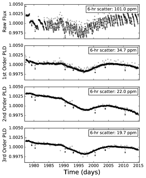
In Figure 1, we illustrate the de-trending technique for EPIC 201367065 (K2-3), a star host to three known transiting planets (Crossfield et al., 2015). The top panel shows the normalized raw aperture-summed flux after subtracting off the background; note the large systematics at very short ($\sim$ 6 hr) timescales. The next panel shows the flux de-trended with first order PLD (Equation 1). The scatter is reduced by a factor of 2.9 and the seven transits become visible by eye. The following two panels show the results of second and third order PLD, which improve the scatter over the raw data by factors of 4.7 and 5.2, respectively. Note, importantly, that even data collected during thruster fire events (the outlier points seen above the continuum every $\sim$ 6 hr in the top two plots), is properly corrected by higher order PLD.

One might wonder why not go to even higher order in the pixel coefficients. While possible in principle, the number of regressors increases steeply with the PLD order. For a typical K2 star, this number is around $5\times 10^{3}$ for third order PLD, and would increase to $\sim 5\times 10^{4}$ for fourth order and $\sim 3\times 10^{5}$ for fifth order PLD. While such a large number of regressors can become computationally expensive, the most serious drawback of higher order PLD is that it can become so flexible as to lead to overfitting. As we discuss in §3.3 below, PLD can sometimes overstep and remove part of the white noise component of the light curve. This is particularly problematic when the number of regressors becomes very large, in which case PLD can lead to artificially low scatter in the de-trended light curve, washing out astrophysical signals (including transits) in the process.

To avoid these issues, in Figure 1 we computed the PLD basis vectors from the 10 brightest pixels in the aperture. In practice, however, we obtain better results by instead performing principal component analysis (PCA) on the first, second, and third order fractional pixel fluxes (the terms in Equation 2.2). This gives us a set of $N$ basis vectors $\mathbf{x}$ that describe most of the instrumental variability in the light curve. We use these to construct our design matrix

$$\mathbf{X}=\begin{pmatrix}x_{0,0}&x_{0,1}&...&x_{0,N}&1\\ \\ x_{1,0}&x_{1,1}&...&x_{1,N}&1\\ \\ ...&...&...&...&...\\ \\ x_{M,0}&x_{M,1}&...&x_{M,N}&1\\ \end{pmatrix}$$ (6)

where $M$ denotes the total number of data points along the time dimension. We choose the number of principal components $N$ that maximize the de-trending power while preventing overfitting. We explain our method in §3.3 below; typically, $N<200$.

Since our problem is still linear, our model is simply

$$\mathbf{m}=\mathbf{X}\cdot\mathbf{c}$$ (7)

where $\mathbf{c}$ is the vector of coefficients, one for each basis vector in $\mathbf{X}$. Their values are given by solving the generalized least-squares (GLS) problem

$$\mathbf{c}=\left(\mathbf{X}^{\top}\cdot\mathbf{K}^{-1}\cdot\mathbf{X}\right)^{-1}\cdot\left(\mathbf{X}^{\top}\cdot\mathbf{K}^{-1}\cdot\mathbf{y}\right)$$ (8)

where $\mathbf{K}$ is the covariance matrix of the data and $\mathbf{y}$ is the SAP flux given by Equation (4). Note that for a diagonal covariance $\mathbf{K}_{ij}=\delta_{ij}\sigma_{i}^{2}$, Equation (8) is mathematically equivalent to Equations (2) and (3) from before.

Figure 1.— PLD applied to a portion of the data for EPIC 201367065 (K2-3). The top panel is the background-subtracted, normalized SAP flux in a large 35-pixel aperture centered on the target. The bottom three panels show the normalized PLD-de-trended flux for 1^st, 2^nd, and 3^rd order PLD, respectively, using only the 10 brightest pixels. PLD increases the 6-hr photometric precision by factors of 2.9 (1^st order), 4.7 (2^nd order), and 5.2 (3^rd order).

2.3. Gaussian Process Regression

Figure 2.— Different de-trending techniques for quarter 4 of KIC 8583696 (KOI 1275), a planet candidate host from the original Kepler mission. The original data are shown in the left column; in the other columns we artificially injected a sinusoidal signal with a period of 25 days and an amplitude comparable to that of the instrumental variability. The top row shows the raw SAP data (black) and the first order PLD model (red); the residuals of the fit are indicated directly below. The third row shows the final residuals after smoothing with a GP to eliminate low-frequency stellar variability. Finally, the bottom row shows these residuals folded on the orbital period of the planet candidate (black), with the 1-hr median indicated in red. Combining PLD with a GP ensures PLD fits out only the instrumental variability without inflating the white noise.

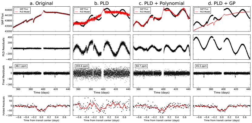
In Equation (6) we purposefully neglected the temporal polynomial terms. In principle, modeling stellar variability should not be necessary if all we wish to remove is the instrumental noise. By virtue of using the fractional pixel fluxes as basis vectors (from which the astrophysical signal has been removed by the normalization), PLD should fit out instrumental variability only, obviating the need for an extra temporal term. However, in practice, this is not always the case. To illustrate this, in Figure 2 we plot a quarter of data of KOI 1275, a star with one planet candidate discovered by the original Kepler mission (Borucki et al., 2011). We chose this star over one from the K2 mission simply because it is easier to discriminate between instrumental and astrophysical signals by eye for this light curve, though our arguments apply equally well to K2.

Figure 2a shows the raw simple aperture photometry (SAP) data in black (top panel); in red we plot a simple first-order PLD fit with no polynomial term (obtained from the solution to Equation 2). Below it are the residuals of the PLD fit (second panel, black) and the fully de-trended data after smoothing with a GP to remove stellar noise (third panel). The bottom panel shows the de-trended data folded on the period of the planet candidate, with the 1-hr median shown in red. Note that the PLD fit is quite good, as it removes the low-frequency arc as well as the flux jump at $t\sim 375$ d and the thermal features at $t\sim 385$ d and $t\sim 400$ d. Since the star isn’t significantly variable, the temporal term is not necessary.

However, this is not the case when the star is variable. In the next three columns we multiply the pixel level light curve by a sinusoid with a period of 25 days to simulate stellar variability. We choose an amplitude comparable to the amplitude of the instrumental signal, and de-trend the light curve three different ways: PLD only (b), PLD plus a tenth order polynomial (c) and PLD plus a GP (d).

The PLD-only fit (Figure 2b) is quite poor. The general shape of the PLD curve is mostly preserved and, as expected, the stellar signal is still present in the residuals, but the fit increases the white noise by a factor of $\sim$ 4, all but washing out the transits (bottom panel). This happens because of a serious limitation of the LLS problem framed in Equation 2, which yields the PLD coefficients that minimize the scatter of the PLD term $m_{i}$ about the flux $y_{i}$. If $m_{i}$ is not a suitable approximation to the flux, as in the case of a highly variable star, the $\chi^{2}$ of the fit will necessarily be large. It is not hard to show that $\chi^{2}$ can be substantially reduced by inflating the white noise component of $m_{i}$, leading to the large scatter seen in the de-trended data. Absent a model for the astrophysical variability, PLD naturally exchanges correlated noise for white noise, which severely compromises its de-trending power.

A straightforward way to improve the quality of the fit is to include the polynomial term to capture the stellar variability, as in Deming et al. (2015). We do this in Figure 2c, where we use a tenth order polynomial. While the fit is significantly improved, PLD still inflates the white noise component, since the polynomial is not flexible enough to capture all of the stellar signal. Though the transit is visible in the bottom plot, the quality of the de-trended data is significantly degraded when compared to that of the non-variable star.

One might imagine that a higher order polynomial would do the trick. However, there is an alternate approach, one that naturally follows from Equation 8. Rather than model the stellar signal explicitly, we instead treat it non-parametrically by performing Gaussian process regression, in which we use a GP to estimate the covariance matrix $\mathbf{K}$. Provided $\mathbf{K}$ is a reasonable approximation to the true covariance of the stellar signal, Equation 8 will yield a set of PLD coefficients that fit out only the instrumental component of the noise. We illustrate this in Figure 2d, where we use a Matérn-3/2 kernel (see Equation 3.2 below) with amplitude $\alpha_{m}=100$ and timescale $\tau_{m}=20$ days to model the stellar signal. Unlike in the previous two cases, the PLD model (top panel, red) no longer attempts to fit out the stellar signal; in fact, the curve is almost identical to the fit to the original data (Figure 2a). The astrophysical signal is recovered to high fidelity by subtracting the PLD term (second panel). After removing it, the final residuals (third panel) show a comparable (in fact, marginally smaller) RMS to the residuals of the original data. It is also clear from the bottom panel that the transit shape and depth are well preserved.

We note that another advantage of GP regression is that the PLD model is relatively insensitive to the particular choice of kernel function and values of its hyperparameters. This can be seen in the example above; even though the stellar variability signal was generated from a 25-day period sinusoidal function, a radial Matérn-3/2 kernel with a timescale of 20 days was sufficient to ensure the instrumental signal was removed without inflating the white noise. This is important because the stellar signal is generally unknown a priori, and any attempt to estimate it from the data will be subject to how well one can discriminate between instrumental and stellar effects.

Finally, we caution that GP regression assumes Gaussian noise. Deviations from Gaussianity, such as the presence of outliers, can invalidate the assumptions of the method and lead to poor fits to the data. Although we remove outliers prior to optimizing the GP, users accessing our de-trended light curves are encouraged to check for Gaussianity with methods such as an Anderson-Darling test. In §3 we describe our iterative procedure for removing outliers and optimizing the GP kernel.

3. Methods

In §2 we outlined the basics of principal component regression on the fractional pixel fluxes using a GP. In this section, we describe how we apply this method to K2 data.

3.1. Pre-Processing

For each star in the K2 EPIC catalog, we download the target pixel files and select aperture number 15 from the K2SFF catalog (Vanderburg & Johnson, 2014; Vanderburg, 2014), which is derived by fitting the Kepler pixel response function (PRF) to the stellar image. The K2SFF data contain twenty such apertures of varying sizes for each star. We find that aperture 15 is typically the best compromise between having enough pixels to generate a good basis set for PLD while preventing excess contamination from neighboring stars. We note that when contamination is not an issue, the choice of aperture has little effect on our results. As in Vanderburg & Johnson (2014), we then compute the median per-timestamp flux in the pixels of the image that lie outside the aperture and subtract it from all pixels to remove the background signal. In this paper, we consider only the long cadence (LC) K2 dataset.

Next, we perform iterative sigma-clipping to mask large outliers. Just as PLD can artificially inflate the white noise in an attempt to remove stellar variability (§2.3), it can do so in the presence of short timescale features such as eclipses, transits, flares, or cosmic ray hits. Deming et al. (2015) deal with this by explicitly adding a transit term to the PLD model (Equation 1), but this requires knowledge of the transit parameters. Since we do not know a priori whether there are transits in a given light curve, we instead mask all features in the light curve that are not well modeled by either the PLD terms or the GP. We then train our model on the masked light curve to compute the PLD coefficients and use those to de-trend the full, unmasked light curve.

We detect outliers by dividing the light curve into five chunks and de-trending each with a first order PLD model. We use a 2-day Matérn-3/2 covariance (see §3.2) with amplitude equal to the median standard deviation of the flux in all 2-day segments; again, we note that our results are relatively insensitive to the particular value of these parameters. Next, we perform a median absolute deviation (MAD) cut at 5$\sigma$ to identify outliers. We then re-compute the PLD model by masking those outliers and de-trend the full light curve, identifying a new set of outliers. This process is repeated until no new outliers are identified. We find that this identifies deep transits, eclipses, and other outliers that could affect the quality of the PLD fit.

3.2. GP Optimization

Figure 3.— GP optimization procedure for EPIC 201497682. In the top left panel we plot the raw SAP flux (black) and a ten chunk, first order PLD fit (red); the residuals are shown in the panel below. These are used to compute the power spectrum of the stellar signal (top right), and its autocorrelation function (bottom right, black curve). Different kernels are then fit to the autocorrelation function, and the one with the lowest $\chi^{2}$ value is chosen for the de-trending step (red curve). The grey envelope about the autocorrelation curve is the ad hoc standard error assumed to compute $\chi^{2}$.

The next step is to compute the covariance matrix $\mathbf{K}$, which we do using the george Python package (Ambikasaran et al., 2016). We parametrize it as

$$\mathbf{K}_{ij}=k_{w}(t_{i},t_{j})+k_{t}(t_{i},t_{j})$$ (9)

where

$$k_{w}(t_{i},t_{j})=\sigma^{2}\delta_{ij}$$ (10)

is a white noise kernel with standard deviation $\sigma$ and $k_{t}$ is either an additive or multiplicative combination of one or more of an exponential kernel $k_{e}$, a Matérn-3/2 kernel $k_{m}$, and a cosine kernel $k_{c}$:

$$k_{e}(t_{i},t_{j}) =\alpha_{e}e^{-\left|t_{i}-t_{j}\right|/\tau_{e}}$$

$$k_{m}(t_{i},t_{j}) =\alpha_{m}\left(1+\sqrt{3(t_{i}-t_{j})^{2}}\right)e^{-\sqrt{3(t_{i}-t_{j})^{2}}/\tau_{m}}$$

$$k_{c}(t_{i},t_{j}) =\alpha_{c}\cos{\left(\frac{2\pi}{P}(t_{i}-t_{j})\right)}.$$ (11)

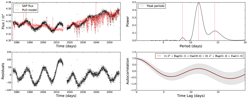
The choice of kernel depends on the properties of the stellar signal, which we do not know a priori, since it is mixed with the instrumental signal in the light curve. We therefore adopt an iterative procedure, where we guess at the initial kernel form and hyperparameters and use it to de-trend the light curve with PLD, thus obtaining an approximate stellar component. We then train the GP on this stellar component and use it to run our PLD analysis again. While this can be repeated multiple times, we find that two iterations are typically enough for most targets. This procedure is illustrated in Figure 3.

Our initial kernel is a Matérn-3/2 kernel with $\tau_{m}=2$ days and amplitude equal to the median variance in 2-day chunks of the light curve. We split the light curve into 5-10 roughly equal chunks and de-trend each of them with first order PLD using Equations 7 and 8. Since we use first order PLD at this step, we do not perform PCA here. We then compute the autocorrelation function of the de-trended data and perform least-squares fits on different additive and multiplicative combinations of the kernels in Equation 3.2, using the peaks in a Lomb-Scargle periodogram as the initial guess for the periods in the cosine kernels. We choose the kernel and corresponding hyperparameters that result in the best fit and compute its overall amplitude as well as the amplitude of the white noise kernel $k_{w}$ by maximizing the marginal likelihood $\mathcal{L}$ of the data given the model,

$$\log\mathcal{L}=-\frac{1}{2}\mathbf{y}^{\top}\cdot\mathbf{K^{-1}}\cdot\mathbf{y}-\frac{1}{2}\log\left|\mathbf{K}\right|-\frac{n}{2}\log 2\pi$$ (12)

where $\mathbf{y}$ is the de-trended flux and $n$ is the number of data points in $\mathbf{y}$ (Rasmussen & Williams, 2006). In principle, one may optimize the parameters of each of the kernel combinations in this way to obtain the best estimate of the covariance matrix. However, such a procedure is computationally expensive. After considerable experimentation, we find that the method outlined above—which takes on the order of one minute on a single core of a 2.66 GHz machine—is sufficient to ensure PLD removes only the instrumental component of the noise for most targets.

3.3. Design Matrix Optimization

The next step in our pipeline is to construct our design matrix (Equation 6). In order to do so, we must choose the number of PLD principal components to use in the regression. This number must be large enough to capture most of the instrumental variability but not so large as to lead to overfitting. In fact, one must take care to prevent PLD (or any other de-trending technique) from fitting out the white noise component of the light curve. As the number of basis vectors grows to become very large, there begin to exist linear combinations of these vectors that can artificially remove white noise from the data, improving the apparent quality of the fit but leading to spurious results. This is best illustrated by considering the example in Figure 1, where we kept only 285 basis vectors in the bottom panel. Had we de-trended with all 8435 components, we would obtain the light curve shown in Figure 4.

Figure 4.— Top: Third order PLD applied to EPIC 201367065, but this time keeping all basis vectors. Compare to Figure 1. While the median scatter improved by a factor of about 4, the scatter in the transits (which were masked during the de-trending) increased by a factor of several thousand. Bottom: The same figure, but zoomed out to show the in-transit scatter.

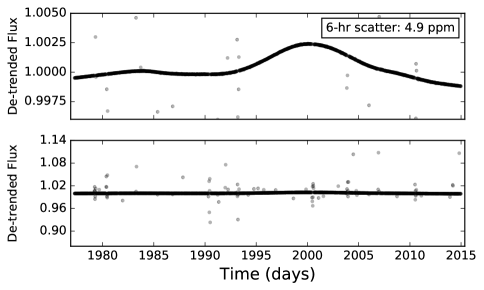
While the median scatter improved by a factor of $\sim$ 4, the in-transit scatter increased by a factor of several thousand. This is because we masked the transits of K2-3b, c, and d during the de-trending step (see §3.1). The poor performance of the extrapolated model betrays its terrible predictive power, a clear sign of overfitting.

In order to limit the flexibility of our PLD model, we implement a simple cross-validation scheme. We divide the light curve into training sets (large chunks of data that we use to compute the PLD coefficients) and validation sets (small randomly selected chunks that we de-trend using the coefficients computed from the training sets). We then compute the 6-hr precision in the validation sets for a range of design matrix sizes (details below). Since the validation data is never used to compute the PLD coefficients, the model cannot overfit in the validation set. Instead, as the number of regressors becomes too large and PLD begins to fit out astrophysical signals and/or white noise, the scatter in the validation set will grow. This process is illustrated in Figure 5, where we plot the scatter in the training set (blue) and the scatter in the validation set (red) as a function of the number of principal components $n_{pc}$.

Figure 5.— De-trended light curve precision as a function of the number of principal components for EPIC 201497682. The blue dots are the median 6-hr precision (in ppm) of the unmasked sections of the light curve (the training set); the red dots are the median precision in 6-hr chunks that were masked during the de-trending step (the validation set). Solid curves indicate our GP fit to the data points. Initially, the scatter decreases in both cases as the number of components is increased. However, above $\sim$ 50 components, while the scatter in the training set continues to decrease, the scatter in the validation set (where the model is extrapolated) begins to grow. This is the signature of overfitting. We therefore choose 50 principal components for the de-trending, yielding a precision of 55 ppm (versus $\sim$ 70 ppm for the K2SFF de-trended flux).

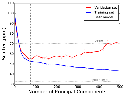
Initially, as $n_{pc}$ increases, the scatter in both the training and validation data decreases. As the number of components increases further, the training precision continues to improve, eventually surpassing the photon noise limit for $n_{pc}\gtrsim 1000$. This is obviously unphysical and a clear sign of overfitting. The scatter in the validation set, on the other hand, begins to increase steadily above $n_{pc}\sim 50$, indicating that the predictive power of the model worsens as the number of principal components is increased. The minimum in the red curve, which occurs for $n_{pc}\sim 80$, is the best we can do; above that point, PLD is likely to begin fitting out white noise.

We employ this cross-validation method for each EPIC target. In practice, we compute the 6-hr precision (see §4.3) in the validation sets fifty times for each value of $n_{pc}$ and take the median. Each validation set is a group of 10 non-overlapping chunks that are masked when computing the PLD coefficients; each chunk is chosen randomly from the set of all contiguous 13-cadence segments of the light curve. Our grid in $n_{pc}$ typically ranges from 1 to 250 principal components, with a spacing of ten components. After computing the median scatter for each value of $n_{pc}$, we smooth the curves with a GP and choose the value of $n_{pc}$ that minimizes the scatter in the validation set.

Finally, for campaign 1 we found it necessary to split all light curves into two separate timeseries, with a breakpoint at $\mathrm{BJD}-2454833=2017$, a mid-campaign data gap. Inspection of the top left panel of Figure 3 reveals a qualitative change in the instrumental systematics in the second half of the campaign, likely due to a reversal in the direction of the spacecraft roll (see, e.g., Aigrain et al., 2016). While similar reversals are also present in other campaigns, campaign 1 is the only one in which we obtain a de-trending improvement significant enough to justify the breakpoint.

3.4. De-trending

After optimizing the GP and choosing the order of the PLD, the number of principal components, and the number of light curve subdivisions, we de-trend each EPIC light curve by subtracting the model given by Equations 7 and 8. We then add the median value of the SAP flux to the result to obtain our final, de-trended light curves.

4. Results

4.1. Transit Injections

Since the PLD basis vectors are obtained from the fractional pixel fluxes, they do not in principle contain any astrophysical signals. De-trending with PLD should therefore preserve the transit shape and depth, a fact that is confirmed for the transits of several hot Jupiters observed with Spitzer (Deming et al., 2015). However, as we showed in §3.3, PLD can increase the scatter of regions of the data that are not used to compute the coefficients (such as transits that are flagged as outliers) when too many principal components are present (see Figure 4). If a transit is missed in the outlier detection step, the transit shape may also be affected, since PLD can exploit linear combinations of the white noise component to decrease the transit depth and therefore improve the likelihood of the fit.

Figure 6.— Transit injection results. Each panel shows the fraction of transits recovered with a certain depth ratio $D/D_{0}$ (recovered depth divided by true depth). Blue histograms correspond to the actual injection and recovery process performed with our pipeline; red histograms correspond to transits injected directly into the de-trended light curves and are shown for comparison. The values to the left and right of each histogram are the median $D/D_{0}$ for our pipeline and for the control run, respectively. The smaller values at the top indicate the fraction of transits recovered with depths lower and higher than the bounds of the plots. Finally, the two columns distinguish between the default runs (left) and runs where the transits were explicitly masked (right); the three rows correspond to different injected depths: $10^{-2}$, $10^{-3}$, and $10^{-4}$. PLD preserves transit depths if the transits are properly masked; otherwise, a small bias toward smaller depths is introduced.

In order to test whether our pipeline is robust against these effects, we ran a set of transit injection and recovery tests on a sample of EPIC targets that do not contain known transit events. We randomly selected 200 campaigns 0-6 stars from each magnitude bin in the range $8\leq K_{p}\leq 18$ ($K_{p}$ is the Kepler bandpass magnitude) for a total sample size of 2000 stars per run. We then injected synthetic transits of varying depths into the light curve by multiplying each pixel by a transit model generated by the pysyzygy package, which calculates fast limb-darkened light curves based on the Mandel & Agol (2002) transit model. We randomly chose orbital periods in the range 3-10 days and fixed the transit duration at 2.5 hours, assuming zero eccentricity and quadratic limb darkening parameters $a=0.45$ and $b=0.30$. We then ran our pipeline to de-trend the light curves.

Performing a full transit search is outside the scope of this paper. Since our goal is to determine whether or not PLD can bias transit depths, we fix all the parameters except for the depth at their true values and recover the transit depth by linear regression, simultaneously fitting the baseline flux in the vicinity of the transit with a third-order polynomial. Our results are shown in Figure 6.

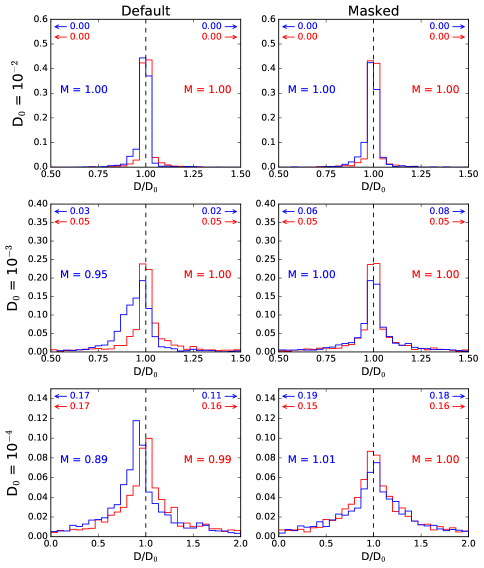
Each panel shows two histograms of the recovered depth as a fraction of the true depth, $D/D_{0}$. In blue, we plot the recovery results after de-trending with our pipeline. As a control, we also injected transits directly into the de-trended data; we plot the corresponding distributions in red. Provided EVEREST does not affect transit depths or increase in-transit scatter, these two sets of distributions should be similar. The numbers at the top left and right of each panel respectively indicate the fraction of recovered depths below and above the limits of the plot. The median values $M$ of each distribution are also shown.

Each row in the figure corresponds to a different injected depth: $10^{-2}$, $10^{-3}$, and $10^{-4}$, ranging from a typical hot Jupiter to a roughly Earth-sized planet. The left column corresponds to the default runs of our pipeline; the right column corresponds to runs in which the transits were explicitly masked (more details on this below).

In the top left panel ($D_{0}=10^{-2}$), both distributions have medians equal to 1.00, corresponding to an unbiased recovery of the transit depth. Moreover, the spread is similar in both distributions, indicating that EVEREST does not introduce significant in-transit scatter. In the next two panels ($D_{0}=10^{-3}$ and $10^{-4}$), however, a bias toward smaller transit depth is visible; the EVEREST de-trending causes transits of these small planets to be shallower by $\sim 5$ and $\sim 10\%$, respectively. This is because our sigma-clipping outlier detection technique (§3.1) is not effective at finding shallow transits, and thus these transits are not masked during the de-trending step. As we mentioned above, since we have no term in our design matrix (Equation 6) to explicitly model transits, the PLD model picks up the slack and partially fits out these features by inflating the white noise, slightly improving the quality of the overall fit. This is similar to the example in Figure 2, where PLD inflated the white noise to remove an astrophysical signal.

When the transits are properly masked (right column of the figure), both the bias and the increased scatter in the recovered depths disappear for transits of all depths. This shows that our cross-validation technique (§3.3) is correctly preventing overfitting and enforcing the high predictive power of the model in the masked regions of the dataset.

In order to remove the small bias introduced in the presence of shallow, unmasked transits, we strongly encourage those making use of our light curves for transiting exoplanet characterization to run EVEREST while explicitly masking these transits. This can be done by specifying the transit times and durations when calling the EVEREST Python module; the code takes only a few seconds to run. The same applies to those using our light curves for transiting planet searches. Once features of interest are detected, one should run EVEREST again with those features masked to obtain unbiased estimates of the transit parameters.

It is important to note, however, that some transits with very low signal-to-noise could be completely fit out during the de-trending step, preventing their detection in the first place. As Foreman-Mackey et al. (2015) point out, this is an inevitable consequence of the de-trend-then-search method. It is always best to use a model that captures all the features of the data, allowing one to solve for instrumental noise, stellar variability, and transits simultaneously. To this end Foreman-Mackey et al. (2015) explicitly include a transit model in their design matrix, solving Equation 8 over a fine grid of periods and transit epochs. This eliminates the de-trending step in favor of a combined de-trending/planet searching step, which effectively circumvents the overfitting problems inherent to least-squares de-trending techniques. However, such an approach is very computationally expensive, given that each light curve must be processed once for every combination of transit parameters. We therefore defer this procedure to a future paper.

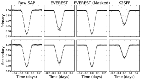
We note, finally, that other K2 pipelines are subject to similar overfitting problems. Consider the example in Figure 7, which shows the (folded and normalized) primary and secondary eclipses of the eclipsing binary EPIC 202072563. Four datasets are presented: the raw SAP flux (left), the default EVEREST light curve, the masked EVEREST light curve, and the K2SFF light curve. The EVEREST and K2SFF fluxes have been smoothed with a GP to remove astrophysical variability. It is clear from the second column that our outlier detection technique failed to mask all points during the eclipse, leading to a $\sim 20\%$ decrease in the eclipse depths. When properly masking the eclipses, however, the depth is correctly recovered (third column). In the last column, we see that the K2SFF depths are also shallower, but by nearly $50\%$. Proper modeling or masking of these features would be necessary to preserve their depths during the K2SFF de-trending step.

Figure 7.— Primary and secondary eclipses of EPIC 202072563, folded on a period of 2.1237 days. From left to right, the columns show the raw SAP flux, the EVEREST flux, the EVEREST flux obtained when explicitly masking the eclipses, and the K2SFF flux. Masking is critical to preserving the transit depth during de-trending for any pipeline that does not explicitly include a transit or eclipse model.

4.2. Limitations

We find that there are two particular situations in which PLD is likely to fail: saturated stars and crowded apertures. These limitations are inherent to the method itself and not specific to K2 data.

4.2.1 Saturated Stars

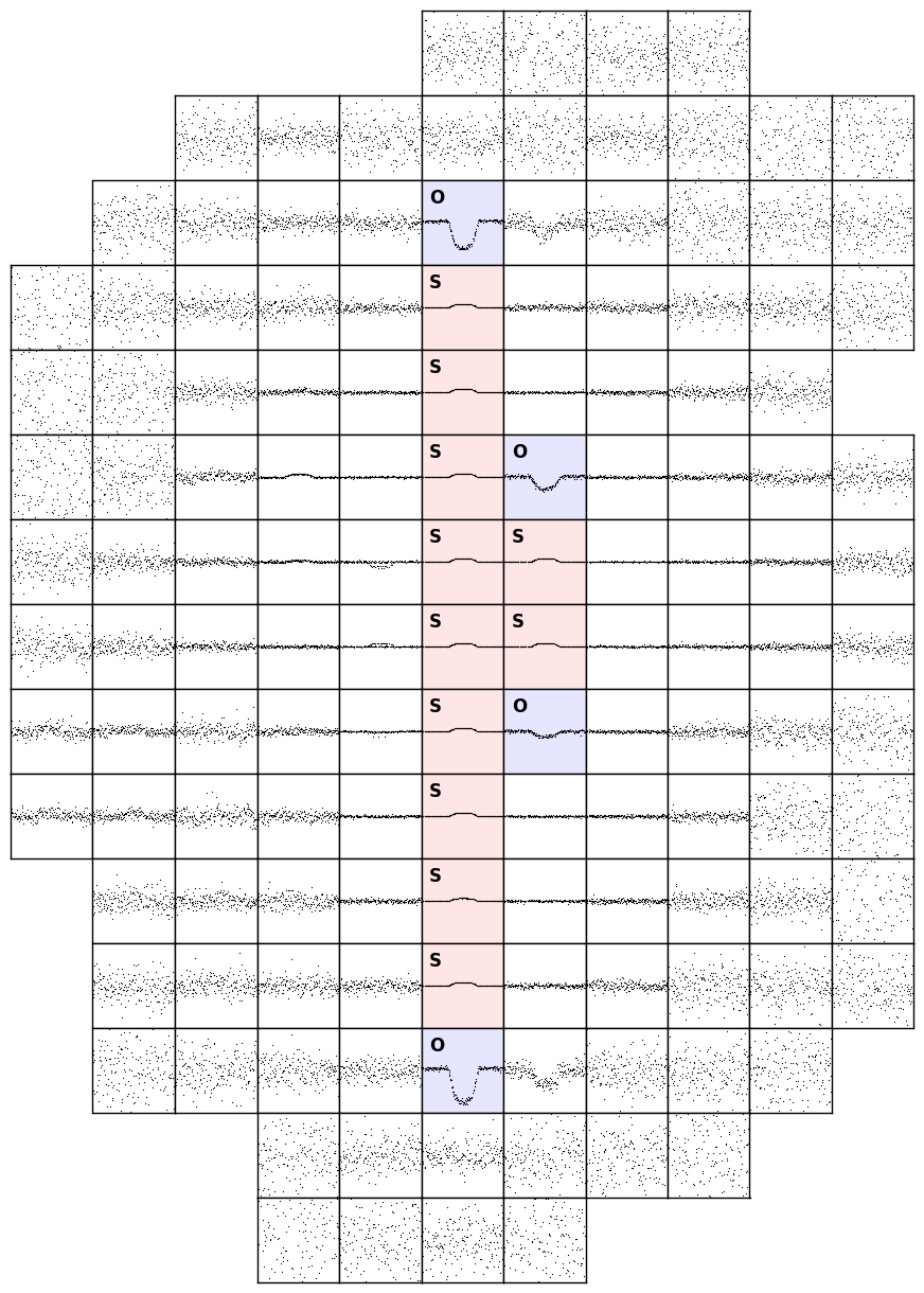
The Kepler detectors begin to saturate for stars with $K_{p}\lesssim 11.5$, leading to flux bleeding along the pixel columns (Gilliland et al., 2010). Since the total charge is well conserved for stars dimmer than $K_{p}\approx 7$, this is not an issue for aperture photometry; transit depths and shapes are preserved in the SAP flux. However, the basic assumption of PLD—that the fractional pixel fluxes $p_{il}/\sum_{k}{p_{ik}}$ (see Equation 2.2) contain no astrophysical information—breaks down for these stars. This occurs because saturated pixels contain virtually no transit signal, as both the in-transit flux and the out-of-transit flux are above the saturation level, resulting in a relatively featureless timeseries. Since the total flux is conserved, the transit signal overflows into the adjacent pixels, traveling along the column until it reaches an unsaturated pixel. In these “overflow” pixels, the fractional transit depth is much larger than the true depth, since it contains the total transit signal from all of the saturated pixels in that column. Consequently, the normalization $p_{il}/\sum_{k}{p_{ik}}$ will only partially remove the transit in the “overflow” pixels. Conversely, it will over-correct the saturated pixel fluxes, leading to an inverted transit shape in the PLD basis vectors corresponding to those pixels. This is illustrated in Figure 8, which shows the fractional pixel fluxes as a function of their position on the detector for the saturated hot-Jupiter host Kepler-3b. We again choose a Kepler target for illustrative purposes, though the idea applies equally to K2. Saturated pixels are indicated in red; “overflow” pixels are indicated in blue; both groups of pixels contain the transit signal. Unsurprisingly, PLD fails to properly de-trend this target, removing most of the transit signal along with the instrumental noise.

Figure 8.— Fractional pixel fluxes $p_{il}/\sum_{k}{p_{ik}}$ for quarter 3 of Kepler-3, a $K_{p}=9.2$ hot-Jupiter host observed by the original Kepler mission. The panels are arranged according to the positions of the pixels on the detector, and the data is smoothed and folded on the orbital period of Kepler-3b. Saturated pixels are highlighted in red and are labeled with an S; overflow pixels are highlighted in blue and labeled with an O. PLD fails for this system because the transit signal is present in several of the basis vectors.

Figure 9.— EPIC 201270464, a $K_{p}=9.4$ saturated eclipsing binary. Plotted here is the raw flux (top), the K2SFF flux (center), and the EVEREST flux (bottom). PLD washes out the stellar variability along with most of the eclipses for some saturated stars.

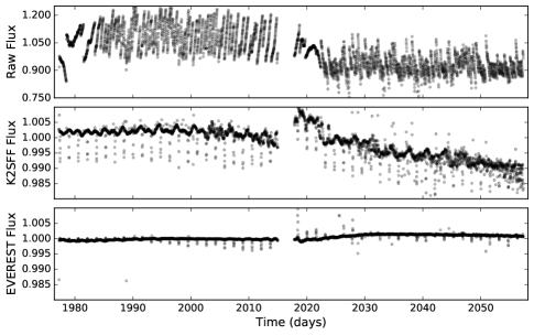
In Figure 9, we show an example of a saturated light curve of an eclipsing binary processed with K2SFF and EVEREST. The K2SFF pipeline removes a significant amount of the instrumental noise while preserving most of the astrophysical signal. EVEREST, on the other hand, fits out both the stellar variability and the eclipses, leading to spurious low scatter.

In principle, the saturation effects may be mitigated by collapsing each saturated column into a single timeseries; since charge is conserved within individual columns, this would enforce the correct transit depth in those “superpixels,” which could then be used as basis vectors for PLD. However, we leave this procedure to future work. At present, we flag saturated stars in our database that are at risk of PLD overfitting. As a general rule, while saturation may occur for stars as faint as $K_{p}=11.5$, we find that PLD preserves transit depths for most stars dimmer than $K_{p}=11$.

4.2.2 Crowded Apertures

The other situation in which PLD performs poorly is in apertures containing significant contamination from other stars. In simple aperture photometry, the transit depth can be decreased in the presence of another star within the aperture. To correct for this, one can simply scale the depth by the (inverse of the) crowding metric, the ratio of the flux due to the planet host to the total flux in the aperture. However, this is not the case for data de-trended with PLD, for reasons we describe below.

In the case of a single star, the pixel flux $p_{il}$ in the $l^{\mathrm{th}}$ pixel at the $i^{\mathrm{th}}$ time is the product of the (position-dependent) stellar signal $a_{il}$ and the (position-independent) transit signal $\tau_{i}$, such that the fractional pixel flux is

$$\frac{p_{il}}{\sum\limits_{k}p_{ik}}=\frac{a_{il}\tau_{i}}{\sum\limits_{k}a_{ik}\tau_{i}}=\frac{a_{il}}{\sum\limits_{k}a_{ik}},$$ (13)

which, as we have argued before, contains no transit signal. In the case of two stars, $a_{il}$ and $b_{il}$, the first of which contains a transit, we may write the fractional flux as

$$\frac{p_{il}}{\sum\limits_{k}p_{ik}}=\frac{a_{il}\tau_{i}+b_{il}}{\sum\limits_{k}a_{ik}\tau_{i}+b_{ik}}.$$ (14)

Note that in this case the transit signal does not cancel, and the PLD basis vectors will contain some amount of transit information, leading to possible overfitting as in the case of a saturated aperture. For a dim contaminant star, $b_{il}\ll a_{il}$, we may write

$$\frac{p_{il}}{\sum\limits_{k}p_{ik}}\approx\frac{a_{il}}{\sum\limits_{k}a_{ik}}\left(1+\frac{\Delta}{\tau_{i}}\right)$$ (15)

where

$$\Delta\equiv\left(\frac{b_{il}}{a_{il}}-\frac{\sum\limits_{k}b_{ik}}{\sum\limits_{k}a_{ik}}\right)$$ (16)

is a measure of the difference between the crowding in a given pixel and the crowding in the entire aperture. In general, the larger the value of $\Delta$, the more power PLD will have to fit out the transit signal. This is the case for bright contaminant sources near the edge of the aperture, for which the value of $b_{il}/a_{il}$ varies greatly across the aperture. Interestingly, for contaminant sources co-located with the transiting planet host (as in the case of binary stars or stars that are aligned but unresolved), the quantity $b_{il}/a_{il}$ is constant across the detector and $\Delta=0$, leading to a PLD basis set that does not contain transit information. This can also be shown from the exact expression (Equation 14). Crowding is therefore only a concern when there is a bright contaminant sufficiently separated from the transiting planet host. In practice, we find that PLD begins to overfit for contaminants that are separated by more than one pixel from the target and are either brighter than or within $\sim 2$ magnitudes of the target.

It is possible to correct for the effects of crowding if the quantity $b_{il}/a_{il}$ is known, even if just approximately. However, this requires careful modeling of the stellar PSF and is beyond the scope of this paper. In our database, we flag sources that may suffer from overfitting due to crowded fields.

4.3. Photometric Precision

The formal photometric noise metric developed by the Kepler team is the Combined Differential Photometric Precision (CDPP) (Christiansen et al., 2012), which is computed by the Kepler pipeline on transit-like timescales of 3, 6 and 12 hours. The CDPP evaluated for a given duration is defined so that it is equivalent to the depth of a transit of that duration that would yield a SNR of 1. In this section we adopt a proxy of the 6-hr CDPP that is easier to calculate than the formal metric defined in Christiansen et al. (2012). Our approach is very similar to the approaches of Gilliland et al. (2011), Vanderburg & Johnson (2014) and Aigrain et al. (2016). In order to prevent correlated stellar noise from inflating the white noise calculation, we apply a 2-day, quadratic Savitsky-Golay (Savitzky & Golay, 1964) high-pass filter to the de-trended flux, clipping outliers at 5$\sigma$. We then compute the standard deviation of all contiguous 13-cadence chunks of data, take the median, and divide by $\sqrt{13}$ as in Vanderburg & Johnson (2014) to obtain the approximate 6-hr photometric precision of the data, which we henceforth refer to as the CDPP.

Figure 10.— 6-hr photometric precision as a function of Kepler magnitude $K_{p}$ for all stars observed by Kepler (yellow dots) and for all unsaturated, non-crowded K2 targets in campaigns 0-7 de-trended with EVEREST (blue dots). The median values are indicated for 0.5 magnitude-wide bins with filled circles. Our pipeline recovers the original Kepler precision for stars brighter than $K_{p}\approx 13$.

Figure 11.— A comparison of the raw K2 6-hr precision (red dots) and the EVEREST precision (blue dots) as a function of $K_{p}$. The lines indicate the median in 0.5 magnitude-wide bins. We also plot the approximate photon limit (dashed yellow line) for reference. EVEREST leads to an order-of-magnitude improvement in the CDPP for the brightest stars.

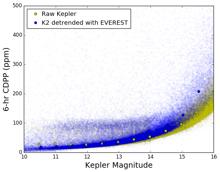
In Figure 10 we plot the CDPP of our de-trended fluxes for campaign 0-7 stars, excluding saturated targets (stars whose brightest pixel’s median flux $>1.6\times 10^{5}\mathrm{e/s}$) and stars in highly crowded apertures (stars with $\Delta K_{p}<5$ neighbors inside the aperture or brighter neighbors within 2 pixels of the edge of the aperture), since PLD is likely to lead to artificially low CDPP in those cases. EVEREST CDPP values are plotted as blue dots. For comparison, in yellow we plot the CDPP calculated for the raw SAP fluxes of all stars observed by the original Kepler mission. EVEREST recovers the raw Kepler CDPP for most $K_{p}\lesssim 13$ stars and yields light curves with CDPP within about 1.5 times that of Kepler for $13\lesssim K_{p}\lesssim 15$. The sparser clump of stars above the bulk group between $K_{p}=11$ and $14$ are likely giants, whose short-timescale pulsations are not efficiently captured by the high-pass filter and thus appear to be more noisy; this clump is also present in the Kepler distribution.

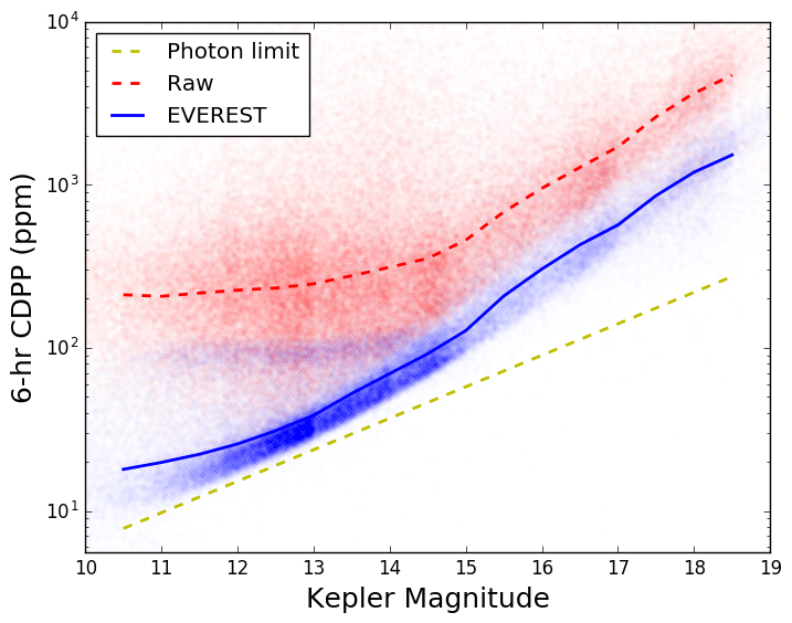
In Figure 11 we again plot the CDPP as a function of $K_{p}$, but this time on a logarithmic scale, comparing the EVEREST values (blue dots) to the raw K2 CDPP (red dots) and the approximate 6-hr photon limit (dashed yellow line), which we calculate as

$$\mathrm{CDPP}_{phot}=\frac{10^{6}}{\sqrt{21600\times\bar{F}}}$$ (17)

where $\bar{F}$ is the average SAP flux in $\mathrm{e/s}$ at a particular value of $K_{p}$. The dashed red and solid blue lines indicate the median CDPP in 0.5 magnitude-wide bins in the raw and de-trended light curves, respectively. EVEREST leads to nearly an order-of-magnitude improvement in the CDPP for the brightest targets, approaching the photon limit for $K_{p}\lesssim 13$ dwarfs.

4.4. Comparison to Other Pipelines

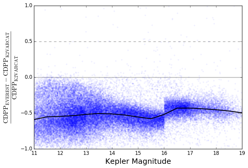
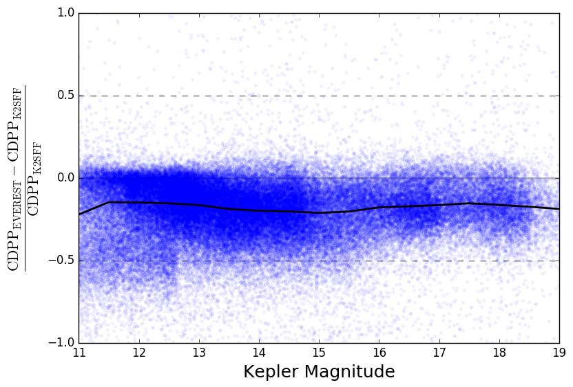
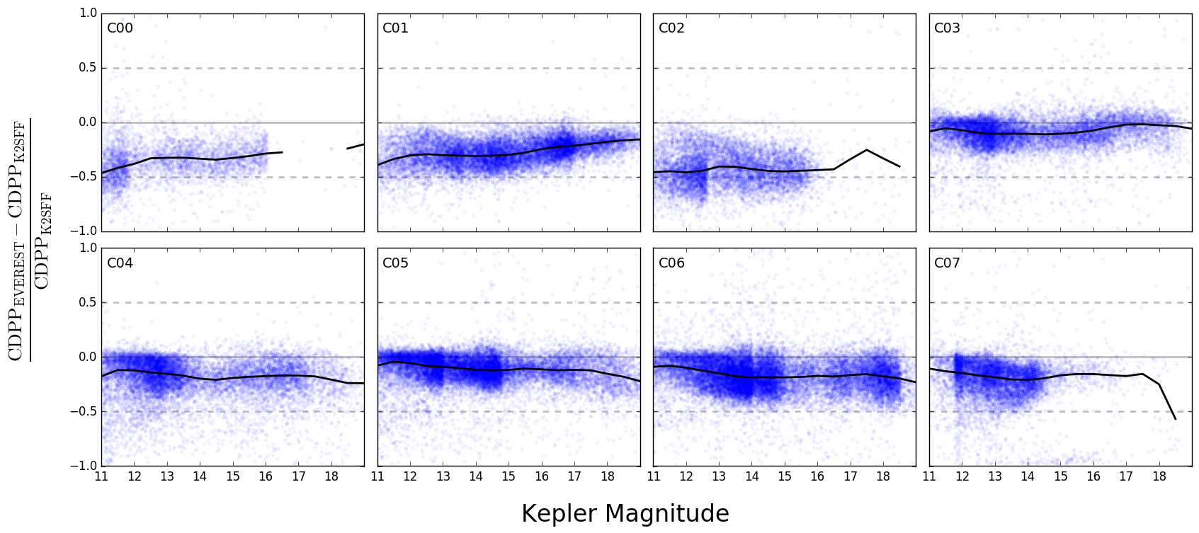
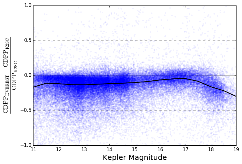
In this section we compare the precision of our de-trended light curves to that of the K2VARCAT (Armstrong et al., 2015), K2SFF (Vanderburg & Johnson, 2014), and K2SC (Aigrain et al., 2016) light curves. Though other pipelines exist (e.g., Lund et al., 2015; Huang et al., 2015; Crossfield et al., 2015), here we focus on those that are also available for download at the MAST HLSP K2 archive. For each of the pipelines, we download all available de-trended light curves and compute the CDPP as described in §4.3. In Figures 12-15, we plot a pairwise comparison of the precision achieved for all campaign 0-7 light curves that are available in both our catalog and that of the other pipeline. These plots are based on Figure 10 in Aigrain et al. (2016); the plots show the relative 6-hr CDPP difference between our light curves and those produced by the K2VARCAT, K2SFF, and K2SC pipelines as a function of Kepler magnitude. Results for individual light curves are indicated by blue dots, and the median in half magnitude-wide bins is shown as a black line. As before, we trim 5$\sigma$ outliers and apply a high-pass filter prior to computing the CDPP. We again exclude from the comparison saturated stars and stars in highly crowded apertures.

Figure 12 shows the comparison to the K2VARCAT pipeline. Our de-trended precision is systematically better at all magnitudes shown; on average, we achieve about double the precision (half the CDPP). There are very few cases where K2VARCAT yields lower CDPP values than EVEREST (points above zero).

Figure 13 shows the same plot, but comparing EVEREST to K2SFF. Again, EVEREST yields higher median precision at all magnitudes; EVEREST light curves have $\sim 20\%$ less scatter on average. The gain in precision changes with $K_{p}$, but also with campaign; this can be seen in Figure 14. Note, in particular, that the EVEREST precision is significantly higher relative to that of K2SFF in campaigns 0-2; in campaign 2, particularly, the average star has half the scatter in the EVEREST light curves. In the more recent campaigns, the precision gain relative to K2SFF is smaller, but EVEREST still yields higher median precision at all magnitudes. In general, EVEREST light curves also have significantly fewer outliers than K2SFF light curves. This is clear from Figures 16 and 17 in the following section: K2SFF light curves often display a band of outliers above or below the light curve continuum, most likely associated with thruster firings. PLD naturally corrects for these, obviating the need to discard the several hundred thruster firing data points in each campaign.

Finally, in Figure 15 we plot the comparison to the PDC version of the K2SC pipeline, whose performance is the best out of the three we consider here. In order to ensure the two datasets are compared on equal footing, we use the systematics-corrected K2SC fluxes rather than the fully whitened fluxes; we obtain these by summing the FLUX and TREND_T columns in the dataset. We then apply a Savitsky-Golay filter, as we do to the EVEREST data, to remove the stellar components of the variability. Since campaigns 0-2 are not available in the K2SC catalog, this plot shows the comparison for campaigns 3-5 only. Once again, EVEREST light curves have higher precision than those of K2SC by $\sim$ 10% for bright stars and $\sim$ 5% for stars in the range $16\lesssim K_{p}\lesssim 11$.

All plots shown here display a significant amount of scatter. While EVEREST yields the lowest median CDPP in all cases, we recommend comparing light curves from the different pipelines when the highest precision is desired for specific targets. Moreover, at this time EVEREST performs poorly for saturated targets and for those in very crowded fields.

Figure 12.— Relative 6-hr CDPP difference between EVEREST and K2VARCAT light curves for campaigns 0-7. Blue dots show differences for individual stars, while the black line indicates the median in 0.5 magnitude-wide bins. Negative values indicate higher precision in the EVEREST light curves; compare to Figure 10 in Aigrain et al. (2016). On average, EVEREST yields light curves with half the scatter for all Kepler magnitudes $K_{p}>11$.

Figure 13.— Same as Figure 12, but comparing EVEREST to K2SFF. Once again, negative values correspond to higher precision in the EVEREST light curves. Our pipeline yields higher precision light curves for most K2 stars and does better on average for all Kepler magnitudes $K_{p}>11$.

Figure 14.— A comparison of the EVEREST and K2SFF CDPP for each individual campaign. Note the marked difference between campaigns 3-7 and campaigns 0-2. For campaign 2, in particular, the relative improvement is close to 0.5, corresponding to an average EVEREST precision a factor of 2 higher than K2SFF.

Figure 15.— Same as Figure 12, but comparing EVEREST to K2SC. To ensure both sets of light curves are on the same footing, the K2SC CDPP is computed from the PDC flux corrected for the instrumental systematics only. As before, a Savitsky-Golay filter is then applied to both sets of light curves. The median relative difference is once again negative everywhere, indicating that EVEREST yields higher precision light curves at all magnitudes.

4.4.1 Example Light Curves

Figure 16.— De-trended light curves for the campaign 1 star EPIC 201367065 (K2-3, Crossfield et al., 2015). Top: The de-trended K2SFF flux (left) and the GP-smoothed flux folded on the periods of the planets b, c, and d (right). Bottom: The de-trended EVEREST flux. The 6-hr CDPP is 30.9 ppm for K2SFF and 16.6 ppm for EVEREST, a factor of $\sim$ 2 improvement.

Figure 17.— De-trended light curves for EPIC 205071984, a campaign 2 star with three known planet candidates (Sinukoff et al., 2015). As in Figure 16, the K2SFF light curve and the folded transits of EPIC 205071984.01 (b), 205071984.02 (c), and 205071984.03 (d) are shown at the top; the equivalent plots for EVEREST are shown at the bottom. The 6-hr CDPP is 56.1 ppm for K2SFF and 24.0 ppm for EVEREST, a factor of $\gtrsim$ 2 improvement.

In Figures 16 and 17 we plot our de-trended light curves for two K2 planet candidate hosts, EPIC 201367065 and 205071984. These were chosen specifically to illustrate the advantages of the PLD technique and are, in a sense, best case scenarios. Both stars have $K_{p}\approx 12$ and are the only bright sources in their apertures. (There are two faint sources, $K_{p}\approx 17$ and $K_{p}\approx 18$, at the edge of the aperture of EPIC 205071984, but they are faint enough as to not affect the de-trending.) In each of the figures, we plot the K2SFF light curves at the top (red) and the EVEREST light curves at the bottom (black). To the right, we plot the folded transits of their planet candidates after removing the stellar variability signal with a GP.

In both cases, the EVEREST precision is a factor of about 2 higher than that of K2SFF: EVEREST yields 30.9 ppm for EPIC 201367065 and 24.0 ppm for EPIC 205071984. This is visible in both the full light curve and in the folded transits, which display significantly less scatter. Note, importantly, that the greater de-trending power of EVEREST does not affect the low-frequency stellar variability, which is present equally in both sets of light curves.

The corresponding light curves in the K2VARCAT database have CDPP values of 43.1 and 63.4, respectively. At the time of writing, these light curves are not present in the K2SC catalog.

5. Conclusions

In this paper we introduced EVEREST, a pipeline developed to yield the highest precision light curves for K2 stars. EVEREST builds on the pixel level decorrelation (PLD) technique of Deming et al. (2015), extending it to third order in the pixel fluxes and combining it with principal component analysis to yield a set of basis vectors that together capture most of the instrumental variability in the data. Gaussian process (GP) regression is then performed to remove the instrumental systematics while preserving astrophysical signals. In order to prevent overfitting, we developed a method to determine the ideal number of principal components to use in the fit, yielding reliable, high precision de-trended light curves for all K2 campaigns to date.

We validated our model by performing transit injection and recovery tests and showed that when transits were properly masked by our iterative sigma-clipping technique, we recovered the correct depths without any bias. When transits were not masked (the case of many low signal-to-noise transits, which are missed by our outlier detection step), PLD de-trending resulted in somewhat shallower transits by $\lesssim 10\%$. We therefore strongly encourage those making use of our light curves for transiting exoplanet characterization to run EVEREST while explicitly masking these transits. Our code is implemented in Python, is user-friendly, and takes only a few seconds to run for a given target. The same applies to those using our light curves for transiting planet searches. Once features of interest are detected, one should run EVEREST again with those features masked to obtain unbiased estimates of the transit parameters. While the decreased transit depth can in principle preclude the detection of very low signal-to-noise planets in the EVEREST light curves, we find that the increased precision of these light curves relative to other pipelines is sufficient to enable the detection of previously unknown, small transiting planets around K2 host stars (Kruse et al., 2016, in prep.). Since EVEREST preserves stellar signals, these light curves should also greatly aid in stellar variability and asteroseismology studies.

For stars brighter than $K_{p}\approx 13$, we found that EVEREST recovers the photometric precision of the original Kepler mission; for fainter stars, the median precision is within a factor of 2 of that of the original mission. We further compared our de-trended light curves to those produced by the other K2 pipelines available at the MAST HLSP K2 archive. EVEREST light curves have systematically higher precision than K2SFF, K2VARCAT and K2SC for all Kepler magnitudes $K_{p}>11$. Currently, EVEREST performs poorly for saturated targets and for those in highly crowded fields.

Our catalog of de-trended light curves is publicly available at https://archive.stsci.edu/prepds/everest/ and will be constantly updated for new K2 campaigns. The code used to de-trend the light curves is open source under the MIT license and is available at https://github.com/rodluger/everest, along with user-friendly routines for downloading and interacting with the de-trended light curves. A static release of version 1.0 of the code is also available at http://dx.doi.org/10.5281/zenodo.56577. Since the only inputs to EVEREST are the pixel level light curves, the techniques developed here can be generally applied to light curves produced by any photometry mission, including the upcoming TESS mission (Ricker et al., 2015), to remove instrumental noise and enable the detection of small transiting planets.

References

- Aigrain et al. (2015) Aigrain, S., Hodgkin, S. T., Irwin, M. J., Lewis, J. R., & Roberts, S. J. 2015, MNRAS, 447, 2880
- Aigrain et al. (2016) Aigrain, S., Parviainen, H., & Pope, B. 2016, ArXiv e-prints
- Ambikasaran et al. (2016) Ambikasaran, S., Foreman-Mackey, D., Greengard, L., Hogg, D. W., & O’Neil, M. 2016, IEEE Transactions on Pattern Analysis and Machine Intelligence, 38, 252
- Armstrong et al. (2015) Armstrong, D. J., Kirk, J., Lam, K. W. F., McCormac, J., Walker, S. R., Brown, D. J. A., Osborn, H. P., Pollacco, D. L., & Spake, J. 2015, A&A, 579, A19
- Borucki et al. (2011) Borucki, W. et al. 2011, ApJ, 736, 19
- Borucki et al. (2013) —. 2013, Science, 340, 587
- Christiansen et al. (2012) Christiansen, J. L., Jenkins, J. M., Caldwell, D. A., Burke, C. J., Tenenbaum, P., Seader, S., Thompson, S. E., Barclay, T. S., Clarke, B. D., Li, J., Smith, J. C., Stumpe, M. C., Twicken, J. D., & Van Cleve, J. 2012, PASP, 124, 1279
- Crossfield et al. (2015) Crossfield, I. J. M., Petigura, E., Schlieder, J. E., Howard, A. W., Fulton, B. J., Aller, K. M., Ciardi, D. R., Lépine, S., Barclay, T., de Pater, I., de Kleer, K., Quintana, E. V., Christiansen, J. L., Schlafly, E., Kaltenegger, L., Crepp, J. R., Henning, T., Obermeier, C., Deacon, N., Weiss, L. M., Isaacson, H. T., Hansen, B. M. S., Liu, M. C., Greene, T., Howell, S. B., Barman, T., & Mordasini, C. 2015, ApJ, 804, 10
- Deming et al. (2015) Deming, D., Knutson, H., Kammer, J., Fulton, B. J., Ingalls, J., Carey, S., Burrows, A., Fortney, J. J., Todorov, K., Agol, E., Cowan, N., Desert, J.-M., Fraine, J., Langton, J., Morley, C., & Showman, A. P. 2015, ApJ, 805, 132
- Foreman-Mackey et al. (2015) Foreman-Mackey, D., Montet, B. T., Hogg, D. W., Morton, T. D., Wang, D., & Schölkopf, B. 2015, ApJ, 806, 215
- Gilliland et al. (2011) Gilliland, R. L., Chaplin, W. J., Dunham, E. W., Argabright, V. S., Borucki, W. J., Basri, G., Bryson, S. T., Buzasi, D. L., Caldwell, D. A., Elsworth, Y. P., Jenkins, J. M., Koch, D. G., Kolodziejczak, J., Miglio, A., van Cleve, J., Walkowicz, L. M., & Welsh, W. F. 2011, ApJS, 197, 6
- Gilliland et al. (2010) Gilliland, R. L., Jenkins, J. M., Borucki, W. J., Bryson, S. T., Caldwell, D. A., Clarke, B. D., Dotson, J. L., Haas, M. R., Hall, J., Klaus, T., Koch, D., McCauliff, S., Quintana, E. V., Twicken, J. D., & van Cleve, J. E. 2010, The Astrophysical Journal Letters, 713, L160
- Howell et al. (2014) Howell, S. B., Sobeck, C., Haas, M., Still, M., Barclay, T., Mullally, F., Troeltzsch, J., Aigrain, S., Bryson, S. T., Caldwell, D., Chaplin, W. J., Cochran, W. D., Huber, D., Marcy, G. W., Miglio, A., Najita, J. R., Smith, M., Twicken, J. D., & Fortney, J. J. 2014, PASP, 126, 398
- Huang et al. (2015) Huang, C. X., Penev, K., Hartman, J. D., Bakos, G. Á., Bhatti, W., Domsa, I., & de Val-Borro, M. 2015, MNRAS, 454, 4159
- Kruse et al. (2016, in prep.) Kruse, E., Luger, R., & Agol, E. 2016, in prep.
- Lund et al. (2015) Lund, M. N., Handberg, R., Davies, G. R., Chaplin, W. J., & Jones, C. D. 2015, ApJ, 806, 30
- Mandel & Agol (2002) Mandel, K. & Agol, E. 2002, ApJ, 580, L171
- Montet et al. (2015) Montet, B. T., Morton, T. D., Foreman-Mackey, D., Johnson, J. A., Hogg, D. W., Bowler, B. P., Latham, D. W., Bieryla, A., & Mann, A. W. 2015, ApJ, 809, 25
- Quintana et al. (2014) Quintana, E. V., Barclay, T., Raymond, S. N., Rowe, J. F., Bolmont, E., Caldwell, D. A., Howell, S. B., Kane, S. R., Huber, D., Crepp, J. R., Lissauer, J. J., Ciardi, D. R., Coughlin, J. L., Everett, M. E., Henze, C. E., Horch, E., Isaacson, H., Ford, E. B., Adams, F. C., Still, M., Hunter, R. C., Quarles, B., & Selsis, F. 2014, Science, 344, 277
- Rasmussen & Williams (2006) Rasmussen, C. E. & Williams, C. K. I. 2006, Gaussian Processes for Machine Learning
- Ricker et al. (2015) Ricker, G. R., Winn, J. N., Vanderspek, R., Latham, D. W., Bakos, G. Á., Bean, J. L., Berta-Thompson, Z. K., Brown, T. M., Buchhave, L., Butler, N. R., Butler, R. P., Chaplin, W. J., Charbonneau, D., Christensen-Dalsgaard, J., Clampin, M., Deming, D., Doty, J., De Lee, N., Dressing, C., Dunham, E. W., Endl, M., Fressin, F., Ge, J., Henning, T., Holman, M. J., Howard, A. W., Ida, S., Jenkins, J. M., Jernigan, G., Johnson, J. A., Kaltenegger, L., Kawai, N., Kjeldsen, H., Laughlin, G., Levine, A. M., Lin, D., Lissauer, J. J., MacQueen, P., Marcy, G., McCullough, P. R., Morton, T. D., Narita, N., Paegert, M., Palle, E., Pepe, F., Pepper, J., Quirrenbach, A., Rinehart, S. A., Sasselov, D., Sato, B., Seager, S., Sozzetti, A., Stassun, K. G., Sullivan, P., Szentgyorgyi, A., Torres, G., Udry, S., & Villasenor, J. 2015, Journal of Astronomical Telescopes, Instruments, and Systems, 1, 014003
- Savitzky & Golay (1964) Savitzky, A. & Golay, M. J. E. 1964, Analytical Chemistry, 36, 1627
- Sinukoff et al. (2015) Sinukoff, E., Howard, A. W., Petigura, E. A., Schlieder, J. E., Crossfield, I. J. M., Ciardi, D. R., Fulton, B. J., Isaacson, H., Aller, K. M., Baranec, C., Beichman, C. A., Hansen, B. M. S., Knutson, H. A., Law, N. M., Liu, M. C., & Riddle, R. 2015, ArXiv e-prints
- Torres et al. (2015) Torres, G., Kipping, D. M., Fressin, F., Caldwell, D. A., Twicken, J. D., Ballard, S., Batalha, N. M., Bryson, S. T., Ciardi, D. R., Henze, C. E., Howell, S. B., Isaacson, H. T., Jenkins, J. M., Muirhead, P. S., Newton, E. R., Petigura, E. A., Barclay, T., Borucki, W. J., Crepp, J. R., Everett, M. E., Horch, E. P., Howard, A. W., Kolbl, R., Marcy, G. W., McCauliff, S., & Quintana, E. V. 2015, ApJ, 800, 99
- Vanderburg (2014) Vanderburg, A. 2014, ArXiv e-prints
- Vanderburg & Johnson (2014) Vanderburg, A. & Johnson, J. A. 2014, PASP, 126, 948