\floatpagestyle

empty

The Multiple Quantile Graphical Model

Alnur Ali1    J. Zico Kolter1,2    Ryan J. Tibshirani1,3
(1Machine Learning Department, Carnegie Mellon University
2Computer Science Department, Carnegie Mellon University
3Department of Statistics, Carnegie Mellon University)
Abstract

We introduce the Multiple Quantile Graphical Model (MQGM), which extends the neighborhood selection approach of Meinshausen and Bühlmann for learning sparse graphical models. The latter is defined by the basic subproblem of modeling the conditional mean of one variable as a sparse function of all others. Our approach models a set of conditional quantiles of one variable as a sparse function of all others, and hence offers a much richer, more expressive class of conditional distribution estimates. We establish that, under suitable regularity conditions, the MQGM identifies the exact conditional independencies with probability tending to one as the problem size grows, even outside of the usual homoskedastic Gaussian data model. We develop an efficient algorithm for fitting the MQGM using the alternating direction method of multipliers. We also describe a strategy for sampling from the joint distribution that underlies the MQGM estimate. Lastly, we present detailed experiments that demonstrate the flexibility and effectiveness of the MQGM in modeling hetereoskedastic non-Gaussian data.

1 Introduction

We consider modeling the joint distribution 𝐏𝐫(y1,,yd)𝐏𝐫subscript𝑦1subscript𝑦𝑑\mathop{\bf Pr}(y_{1},\ldots,y_{d}) of d𝑑d random variables, given n𝑛n independent draws from this distribution y(1),,y(n)Rdsuperscript𝑦1superscript𝑦𝑛superscriptR𝑑y^{(1)},\ldots,y^{(n)}\in{\mbox{\bf R}}^{d}, where possibly dnmuch-greater-than𝑑𝑛d\gg n. Later, we generalize this setup and consider modeling the conditional distribution 𝐏𝐫(y1,,yd|x1,,xp)𝐏𝐫subscript𝑦1conditionalsubscript𝑦𝑑subscript𝑥1subscript𝑥𝑝\mathop{\bf Pr}(y_{1},\ldots,y_{d}|x_{1},\ldots,x_{p}), given n𝑛n independent pairs (x(1),y(1)),,(x(n),y(n))Rp+dsuperscript𝑥1superscript𝑦1superscript𝑥𝑛superscript𝑦𝑛superscriptR𝑝𝑑(x^{(1)},y^{(1)}),\ldots,(x^{(n)},y^{(n)})\in{\mbox{\bf R}}^{p+d}. Our starting point is the neighborhood selection method of Meinshausen and Bühlmann (2006), which is typically considered in the context of multivariate Gaussian data, and seen as a tool for covariance selection (Dempster, 1972): when 𝐏𝐫(y1,,yd)𝐏𝐫subscript𝑦1subscript𝑦𝑑\mathop{\bf Pr}(y_{1},\ldots,y_{d}) is a multivariate Gaussian distribution, it is a well-known fact yjsubscript𝑦𝑗y_{j} and yksubscript𝑦𝑘y_{k} are conditionally independent given the remaining variables if and ony if the coefficent corresponding to yksubscript𝑦𝑘y_{k} is zero in the (linear) regression of yjsubscript𝑦𝑗y_{j} on all other variables (e.g., Lauritzen (1996)). Therefore, in neighborhood selection we compute, for each k=1,,d𝑘1𝑑k=1,\ldots,d, a lasso regression — in order to obtain a small set of conditional dependencies — of yksubscript𝑦𝑘y_{k} on the remaining variables, i.e.,

minimizeθk𝐑di=1n(yk(i)jkθkjyj(i))2+λθk1,subscriptminimizesubscript𝜃𝑘superscript𝐑𝑑superscriptsubscript𝑖1𝑛superscriptsuperscriptsubscript𝑦𝑘𝑖subscript𝑗𝑘subscript𝜃𝑘𝑗superscriptsubscript𝑦𝑗𝑖2𝜆subscriptnormsubscript𝜃𝑘1\mathop{\mbox{minimize}}_{\theta_{k}\in{\bf R}^{d}}\;\sum_{i=1}^{n}\bigg{(}y_{k}^{(i)}-\sum_{j\neq k}\theta_{kj}y_{j}^{(i)}\bigg{)}^{2}+\lambda\|\theta_{k}\|_{1}, (1)

for a tuning parameter λ>0𝜆0\lambda>0. This strategy can be seen as a pseudolikelihood approximation (Besag, 1974),

𝐏𝐫(y1,,yd)k=1d𝐏𝐫(yk|y¬k),𝐏𝐫subscript𝑦1subscript𝑦𝑑superscriptsubscriptproduct𝑘1𝑑𝐏𝐫conditionalsubscript𝑦𝑘subscript𝑦𝑘\mathop{\bf Pr}(y_{1},\ldots,y_{d})\approx\prod_{k=1}^{d}\mathop{\bf Pr}(y_{k}|y_{\neg k}), (2)

where y¬ksubscript𝑦𝑘y_{\neg k} denotes all variables except yksubscript𝑦𝑘y_{k}. Under the multivariate Gaussian model for 𝐏𝐫(y1,,yd)𝐏𝐫subscript𝑦1subscript𝑦𝑑\mathop{\bf Pr}(y_{1},\ldots,y_{d}), the conditional distributions 𝐏𝐫(yk|y¬k)𝐏𝐫conditionalsubscript𝑦𝑘subscript𝑦𝑘\mathop{\bf Pr}(y_{k}|y_{\neg k}), k=1,,d𝑘1𝑑k=1,\ldots,d here are (univariate) Gaussians, and maximizing the pseudolikelihood in (2) is equivalent to separately maximizing the conditionals, as is precisely done in (1) (with induced sparsity), for k=1,,d𝑘1𝑑k=1,\ldots,d.

Following the pseudolikelihood-based approach traditionally means carrying out three steps: (i) we write down a suitable family of joint distributions for 𝐏𝐫(y1,,yd)𝐏𝐫subscript𝑦1subscript𝑦𝑑\mathop{\bf Pr}(y_{1},\ldots,y_{d}), (ii) we derive the conditionals 𝐏𝐫(yk|y¬k)𝐏𝐫conditionalsubscript𝑦𝑘subscript𝑦𝑘\mathop{\bf Pr}(y_{k}|y_{\neg k}), k=1,,d𝑘1𝑑k=1,\ldots,d, and then (iii) we maximize each conditional likelihood by (freely) fitting the parameters. Neighborhood selection, and a number of related approaches that came after it (see Section 2.1), can be all thought of in this workflow. In many ways, step (ii) acts as the bottleneck here, and to derive the conditionals, we are usually limited to a homoskedastic and parameteric family for the joint distribution.

The approach we take in this paper differs somewhat substantially, as we begin by directly modeling the conditionals in (2), without any preconceived model for the joint distribution — in this sense, it may be seen a type of dependency network (Heckerman et al., 2000) for continuous data. We also employ heteroskedastic, nonparametric models for the conditional distributions, which allows us great flexibility in learning these conditional relationships. Our method, called the Multiple Quantile Graphical Model (MQGM), is a marriage of ideas in high-dimensional, nonparametric, multiple quantile regression with those in the dependency network literature (the latter is typically focused on discrete, not continuous, data).

An outline for this paper is as follows. Section 2 reviews background material, and Section 3 develops the MQGM estimator. Section 4 studies basic properties of the MQGM, and establishes a structure recovery result under appropriate regularity conditions, even for heteroskedastic, non-Gaussian data. Section 5 describes an efficient ADMM algorithm for estimation, and Section 6 presents empirical examples comparing the MQGM versus common alternatives. Section 7 concludes with a discussion.

2 Background

2.1 Neighborhood selection and related methods

Neighborhood selection has motivated a number of methods for learning sparse graphical models. The literature here is vast; we do not claim to give a complete treatment, but just mention some relevant approaches. Many pseudolikelihood approaches have been proposed, see, e.g., Rocha et al. (2008); Peng et al. (2009); Friedman et al. (2010); Liu and Wang (2012); Khare et al. (2014); Ali et al. (2016). These works exploit the connection between estimating a sparse inverse covariance matrix and regression, and they vary in terms of the optimization algorithms they use and the theoretical guarantees they offer.

In a related but distinct line of research, Yuan and Lin (2007); Banerjee et al. (2008); Friedman et al. (2008); Rothman et al. (2008) proposed 1subscript1\ell_{1}-penalized likelihood estimation in the Gaussian graphical model, a method now generally termed the graphical lasso (GLasso). Following this, several recent papers have extended the GLasso in various ways. Finegold and Drton (2011) examined a modification based on the multivariate Student t𝑡t-distribution, for robust graphical modeling. Sohn and Kim (2012); Yuan and Zhang (2014); Wytock and Kolter (2013) considered conditional distributions of the form 𝐏𝐫(y1,,yd|x1,,xp)𝐏𝐫subscript𝑦1conditionalsubscript𝑦𝑑subscript𝑥1subscript𝑥𝑝\mathop{\bf Pr}(y_{1},\ldots,y_{d}|x_{1},\ldots,x_{p}). Lee and Hastie (2013) proposed a model for mixed (both continuous and discrete) data types, generalizing both GLasso and pairwise Markov random fields. Liu et al. (2009, 2012) used copulas for learning non-Gaussian graphical models.

A strength of neighborhood-based (i.e., pseudolikelihood-based) approaches lies in their simplicity; because they essentially reduce to a collection of univariate probability models, they are in a sense much easier to study outside of the typical homoskedastic, Gaussian data setting. Höfling and Tibshirani (2009); Yang et al. (2012, 2015) elegantly studied the implications of using univariate exponential family models for the conditionals in (2). Closely related to pseudoliklihood approaches are dependency networks (Heckerman et al., 2000). Both frameworks focus on the conditional distributions of one variable given all the rest; the difference lies in whether or not the model for conditionals stems from first specifying some family of joint distributions (pseudolikelihood methods), or not (dependency networks). Dependency networks have been thoroughly studied for discrete data, e.g., Heckerman et al. (2000); Neville and Jensen (2004). For continuous data, Voorman et al. (2014) proposed modeling the mean in a Gaussian neighborhood regression as a nonparametric, additive function of the remaining variables, yielding flexible relationships — this is a type of dependency network for continuous data (though it is not described by the authors in this way). Our method, the MQGM, also deals with continuous data, and is the first to our knowledge that allows for fully nonparametric conditional distributions, as well as nonparametric contributions of the neighborhood variables, in each local model.

2.2 Quantile regression

In linear regression, we estimate the conditional mean of y|x1,,xpconditional𝑦subscript𝑥1subscript𝑥𝑝y|x_{1},\ldots,x_{p} based on data samples. Similarly, in α𝛼\alpha-quantile regression (Koenker and Bassett, 1978), we estimate the conditional α𝛼\alpha-quantile of y|x1,,xpconditional𝑦subscript𝑥1subscript𝑥𝑝y|x_{1},\ldots,x_{p}, formally Qy|x1,,xp(α)=inf{t:𝐏𝐫(yt|x1,,xp)α}subscript𝑄conditional𝑦subscript𝑥1subscript𝑥𝑝𝛼infimumconditional-set𝑡𝐏𝐫𝑦conditional𝑡subscript𝑥1subscript𝑥𝑝𝛼Q_{y|x_{1},\ldots,x_{p}}(\alpha)=\inf\{t:\mathop{\bf Pr}(y\leq t|x_{1},\ldots,x_{p})\geq\alpha\}, for a given α[0,1]𝛼01\alpha\in[0,1], by solving the convex optimization problem:

minimizeθi=1nψα(y(i)j=1qθjxj(i)),subscriptminimize𝜃superscriptsubscript𝑖1𝑛subscript𝜓𝛼superscript𝑦𝑖superscriptsubscript𝑗1𝑞subscript𝜃𝑗superscriptsubscript𝑥𝑗𝑖\mathop{\mbox{minimize}}_{\theta}\;\sum_{i=1}^{n}\psi_{\alpha}\bigg{(}y^{(i)}-\sum_{j=1}^{q}\theta_{j}x_{j}^{(i)}\bigg{)},

where ψα(z)=max{αz,(α1)z}subscript𝜓𝛼𝑧𝛼𝑧𝛼1𝑧\psi_{\alpha}(z)=\max\{\alpha z,(\alpha-1)z\} is the quantile loss (also referred to as the “pinball” or “tilted absolute” loss). Quantile regression can be useful when the conditional distribution in question is suspected to be heteroskedastic and/or non-Gaussian, e.g., heavy-tailed, or if we wish to understand properties of the distribution other than the mean, e.g., tail behavior. In multiple quantile regression, we solve several quantile regression problems simultaneously, each corresponding to a different quantile level; these problems can be coupled somehow to increase efficiency in estimation (see details in the next section). Again, the literature on quantile regression is quite vast (especially that from econometrics), and we only give a short review here. A standard text is Koenker (2005). Nonparametric modeling of quantiles is a natural extension from the (linear) quantile regression approach outlined above; in the univariate case (one conditioning variable), Koenker et al. (1994) suggested a method using smoothing splines, and Takeuchi et al. (2006) described an approach using kernels. More recently, Koenker (2011) studied the multivariate nonparametric case (more than one conditioning variable), using additive models. In the high-dimensional setting, where p𝑝p is large, Belloni and Chernozhukov (2011); Kato (2011); Fan et al. (2014) studied 1subscript1\ell_{1}-penalized quantile regression and derived estimation and recovery theory for non-(sub-)Gaussian data. We extend results in Fan et al. (2014) to prove structure recovery guarantees for the MQGM (in Section 4.3).

3 The multiple quantile graphical model

Many choices can be made with regards to the final form of the MQGM, and to help in understanding these options, we break down our presentation in parts. First fix some ordered set 𝒜={α1,,αr}𝒜subscript𝛼1subscript𝛼𝑟\mathcal{A}=\{\alpha_{1},\ldots,\alpha_{r}\} of quantile levels, e.g., 𝒜={0.05,0.10,,0.95}𝒜0.050.100.95\mathcal{A}=\{0.05,0.10,\ldots,0.95\}. For each variable yksubscript𝑦𝑘y_{k}, and each level αsubscript𝛼\alpha_{\ell}, we model the αsubscript𝛼\alpha_{\ell}-conditional quantile given the other variables, using an additive expansion of the form:

Qyk|y¬k(α)=bk+jkdfkj(yj),subscript𝑄conditionalsubscript𝑦𝑘subscript𝑦𝑘subscript𝛼subscriptsuperscript𝑏𝑘superscriptsubscript𝑗𝑘𝑑superscriptsubscript𝑓𝑘𝑗subscript𝑦𝑗Q_{y_{k}|y_{\neg k}}(\alpha_{\ell})=b^{*}_{\ell k}+\sum_{j\neq k}^{d}f_{\ell kj}^{*}(y_{j}), (3)

where bkRsuperscriptsubscript𝑏𝑘Rb_{\ell k}^{*}\in{\mbox{\bf R}} is an intercept term, and fkjsuperscriptsubscript𝑓𝑘𝑗f_{\ell kj}^{*}, j=1,,d𝑗1𝑑j=1,\ldots,d are smooth, but not parametric in form.

Generic functional form of the MQGM

In its most general form, the MQGM estimator is defined as a collection of optimization problems, over k=1,,d𝑘1𝑑k=1,\ldots,d and =1,,r1𝑟\ell=1,\ldots,r:

minimizebk,fkjkj,j=1,,di=1nψα(yk(i)bkjkfkj(yj(i)))+jk(λ1P1(fkj)+λ2P2(fkj))ω.subscriptminimizeformulae-sequencesubscript𝑏𝑘subscript𝑓𝑘𝑗subscript𝑘𝑗𝑗1𝑑superscriptsubscript𝑖1𝑛subscript𝜓subscript𝛼superscriptsubscript𝑦𝑘𝑖subscript𝑏𝑘subscript𝑗𝑘subscript𝑓𝑘𝑗superscriptsubscript𝑦𝑗𝑖subscript𝑗𝑘superscriptsubscript𝜆1subscript𝑃1subscript𝑓𝑘𝑗subscript𝜆2subscript𝑃2subscript𝑓𝑘𝑗𝜔\mathop{\mbox{minimize}}_{b_{\ell k},\,f_{\ell kj}\in\mathcal{F}_{\ell kj},\,j=1,\ldots,d}\;\sum_{i=1}^{n}\psi_{\alpha_{\ell}}\bigg{(}y_{k}^{(i)}-b_{\ell k}-\sum_{j\not=k}f_{\ell kj}(y_{j}^{(i)})\bigg{)}+\sum_{j\not=k}\Big{(}\lambda_{1}P_{1}(f_{\ell kj})+\lambda_{2}P_{2}(f_{\ell kj})\Big{)}^{\omega}. (4)

Here λ1,λ20subscript𝜆1subscript𝜆20\lambda_{1},\lambda_{2}\geq 0 are tuning parameters. Also, kjsubscript𝑘𝑗\mathcal{F}_{\ell kj}, j=1,,d𝑗1𝑑j=1,\ldots,d are spaces of univariate functions, ω>0𝜔0\omega>0 is a fixed exponent, and P1,P2subscript𝑃1subscript𝑃2P_{1},P_{2} are sparsity and smoothness penalty functions, respectively, all to be decided as part of the modeling process. We give three examples below; several other variants are possible outside of what we describe.

Example 1: basis expansion model

Consider taking kj=𝐬𝐩𝐚𝐧{ϕ1j,,ϕmj}subscript𝑘𝑗𝐬𝐩𝐚𝐧superscriptsubscriptitalic-ϕ1𝑗superscriptsubscriptitalic-ϕ𝑚𝑗\mathcal{F}_{\ell kj}=\mathbf{span}\{\phi_{1}^{j},\ldots,\phi_{m}^{j}\}, the span of m𝑚m basis functions, e.g., radial basis functions (RBFs) with centers placed at appropriate locations across the domain of variable j𝑗j, for each j=1,,d𝑗1𝑑j=1,\ldots,d. This means that each fkjkjsubscript𝑓𝑘𝑗subscript𝑘𝑗f_{\ell kj}\in\mathcal{F}_{\ell kj} can be expressed as fkj(x)=θkjTϕj(x)subscript𝑓𝑘𝑗𝑥superscriptsubscript𝜃𝑘𝑗𝑇superscriptitalic-ϕ𝑗𝑥f_{\ell kj}(x)=\theta_{\ell kj}^{T}\phi^{j}(x), for a coefficient vector θkjRmsubscript𝜃𝑘𝑗superscriptR𝑚\theta_{\ell kj}\in{\mbox{\bf R}}^{m}, where ϕj(x)=(ϕ1j(x),,ϕmj(x))superscriptitalic-ϕ𝑗𝑥subscriptsuperscriptitalic-ϕ𝑗1𝑥subscriptsuperscriptitalic-ϕ𝑗𝑚𝑥\phi^{j}(x)=(\phi^{j}_{1}(x),\ldots,\phi^{j}_{m}(x)). Also consider an exponent ω=1𝜔1\omega=1, and the sparsity and smoothness penalties

P1(fkj)=θkj2andP2(fkj)=θkj22,formulae-sequencesubscript𝑃1subscript𝑓𝑘𝑗subscriptnormsubscript𝜃𝑘𝑗2andsubscript𝑃2subscript𝑓𝑘𝑗superscriptsubscriptnormsubscript𝜃𝑘𝑗22P_{1}(f_{\ell kj})=\|\theta_{\ell kj}\|_{2}\quad\text{and}\quad P_{2}(f_{\ell kj})=\|\theta_{\ell kj}\|_{2}^{2},

respectively, which are group lasso and ridge penalties, respectively. With these choices in place, the MQGM problem in (4) can be rewritten in finite-dimensional form:

minimizebk,θk=(θk1,,θkd)ψα(Ykbk𝟏Φθk)+jk(λ1θkj2+λ2θkj22).subscriptminimizesubscript𝑏𝑘subscript𝜃𝑘subscript𝜃𝑘1subscript𝜃𝑘𝑑subscript𝜓subscript𝛼subscript𝑌𝑘subscript𝑏𝑘1Φsubscript𝜃𝑘subscript𝑗𝑘subscript𝜆1subscriptnormsubscript𝜃𝑘𝑗2subscript𝜆2superscriptsubscriptnormsubscript𝜃𝑘𝑗22\mathop{\mbox{minimize}}_{b_{\ell k},\,\theta_{\ell k}=(\theta_{\ell k1},\ldots,\theta_{\ell kd})}\;\psi_{\alpha_{\ell}}\Big{(}Y_{k}-b_{\ell k}\mathbf{1}-\Phi\theta_{\ell k}\Big{)}+\sum_{j\not=k}\Big{(}\lambda_{1}\|\theta_{\ell kj}\|_{2}+\lambda_{2}\|\theta_{\ell kj}\|_{2}^{2}\Big{)}. (5)

Above, we used the abbreviation ψα(z)=i=1nψα(zi)subscript𝜓subscript𝛼𝑧superscriptsubscript𝑖1𝑛subscript𝜓subscript𝛼subscript𝑧𝑖\psi_{\alpha_{\ell}}(z)=\sum_{i=1}^{n}\psi_{\alpha_{\ell}}(z_{i}) for a vector z=(z1,,zn)Rn𝑧subscript𝑧1subscript𝑧𝑛superscriptR𝑛z=(z_{1},\ldots,z_{n})\in{\mbox{\bf R}}^{n}, and also Yk=(yk(1),,yk(n))Rnsubscript𝑌𝑘superscriptsubscript𝑦𝑘1superscriptsubscript𝑦𝑘𝑛superscriptR𝑛Y_{k}=(y_{k}^{(1)},\ldots,y_{k}^{(n)})\in{\mbox{\bf R}}^{n} for the observations along variable k𝑘k, 𝟏=(1,,1)Rn111superscriptR𝑛\mathbf{1}=(1,\ldots,1)\in{\mbox{\bf R}}^{n}, and ΦRn×dmΦsuperscriptR𝑛𝑑𝑚\Phi\in{\mbox{\bf R}}^{n\times dm} for the basis matrix, with blocks of columns Φij=ϕ(yj(i))TRmsubscriptΦ𝑖𝑗italic-ϕsuperscriptsuperscriptsubscript𝑦𝑗𝑖𝑇superscriptR𝑚\Phi_{ij}=\phi(y_{j}^{(i)})^{T}\in{\mbox{\bf R}}^{m}.

The basis expansion model is simple and tends to works well in practice. For the majority of the paper, we will focus on this model; in principle, everything that follows (methodologically, theoretically, algorithmically) extends to the next two models we describe, as well as many other variants.

Example 2: smoothing splines model

Now consider taking kj=𝐬𝐩𝐚𝐧{g1j,,gnj}subscript𝑘𝑗𝐬𝐩𝐚𝐧superscriptsubscript𝑔1𝑗superscriptsubscript𝑔𝑛𝑗\mathcal{F}_{\ell kj}=\mathbf{span}\{g_{1}^{j},\ldots,g_{n}^{j}\}, the span of m=n𝑚𝑛m=n natural cubic splines with knots at yj(1),,yj(n)superscriptsubscript𝑦𝑗1superscriptsubscript𝑦𝑗𝑛y_{j}^{(1)},\ldots,y_{j}^{(n)}, for j=1,,d𝑗1𝑑j=1,\ldots,d. As before, we can then write fkj(x)=θkjTgj(x)subscript𝑓𝑘𝑗𝑥superscriptsubscript𝜃𝑘𝑗𝑇superscript𝑔𝑗𝑥f_{\ell kj}(x)=\theta_{\ell kj}^{T}g^{j}(x) with coefficients θkjRnsubscript𝜃𝑘𝑗superscriptR𝑛\theta_{\ell kj}\in{\mbox{\bf R}}^{n}, for fkjkjsubscript𝑓𝑘𝑗subscript𝑘𝑗f_{\ell kj}\in\mathcal{F}_{\ell kj}. The work of Meier et al. (2009), on high-dimensional additive smoothing splines, suggests a choice of exponent ω=1/2𝜔12\omega=1/2, and penalties

P1(fkj)=Gjθkj22andP2(fkj)=θkjTΩjθkj,formulae-sequencesubscript𝑃1subscript𝑓𝑘𝑗superscriptsubscriptnormsuperscript𝐺𝑗subscript𝜃𝑘𝑗22andsubscript𝑃2subscript𝑓𝑘𝑗superscriptsubscript𝜃𝑘𝑗𝑇superscriptΩ𝑗subscript𝜃𝑘𝑗P_{1}(f_{\ell kj})=\|G^{j}\theta_{\ell kj}\|_{2}^{2}\quad\text{and}\quad P_{2}(f_{\ell kj})=\theta_{\ell kj}^{T}\Omega^{j}\theta_{\ell kj},

for sparsity and smoothness, respectively, where GjRn×nsuperscript𝐺𝑗superscriptR𝑛𝑛G^{j}\in{\mbox{\bf R}}^{n\times n} is a spline basis matrix with entries Giij=gij(yj(i))subscriptsuperscript𝐺𝑗𝑖superscript𝑖subscriptsuperscript𝑔𝑗superscript𝑖superscriptsubscript𝑦𝑗𝑖G^{j}_{ii^{\prime}}=g^{j}_{i^{\prime}}(y_{j}^{(i)}), and ΩjsuperscriptΩ𝑗\Omega^{j} is the smoothing spline penalty matrix containing integrated products of pairs of twice differentiated basis functions. The MQGM problem in (4) can be translated into a finite-dimensional form, very similar to what we have done in (5), but we omit this for brevity.

Example 3: RKHS model

Consider taking kj=jsubscript𝑘𝑗subscript𝑗\mathcal{F}_{\ell kj}=\mathcal{H}_{j}, a univariate reproducing kernel Hilbert space (RKHS), with kernel function κj(,)superscript𝜅𝑗\kappa^{j}(\cdot,\cdot). The representer theorem allows us to express each function fkjjsubscript𝑓𝑘𝑗subscript𝑗f_{\ell kj}\in\mathcal{H}_{j} in terms of the representers of evaluation, i.e., fkj(x)=i=1n(θkj)iκj(x,yj(i))subscript𝑓𝑘𝑗𝑥superscriptsubscript𝑖1𝑛subscriptsubscript𝜃𝑘𝑗𝑖superscript𝜅𝑗𝑥subscriptsuperscript𝑦𝑖𝑗f_{\ell kj}(x)=\sum_{i=1}^{n}(\theta_{\ell kj})_{i}\kappa^{j}(x,y^{(i)}_{j}), for a coefficient vector θkjRnsubscript𝜃𝑘𝑗superscriptR𝑛\theta_{\ell kj}\in{\mbox{\bf R}}^{n}. The work of Raskutti et al. (2012), on high-dimensional additive RKHS modeling, suggests a choice of exponent ω=1𝜔1\omega=1, and sparsity and smoothness penalties

P1(fkj)=Kjθkj2andP2(fkj)=θkjTKjθkj,formulae-sequencesubscript𝑃1subscript𝑓𝑘𝑗subscriptnormsuperscript𝐾𝑗subscript𝜃𝑘𝑗2andsubscript𝑃2subscript𝑓𝑘𝑗superscriptsubscript𝜃𝑘𝑗𝑇superscript𝐾𝑗subscript𝜃𝑘𝑗P_{1}(f_{\ell kj})=\|K^{j}\theta_{\ell kj}\|_{2}\quad\text{and}\quad P_{2}(f_{\ell kj})=\sqrt{\theta_{\ell kj}^{T}K^{j}\theta_{\ell kj}},

respectively, where KjRn×nsuperscript𝐾𝑗superscriptR𝑛𝑛K^{j}\in{\mbox{\bf R}}^{n\times n} is the kernel matrix with entries Kiij=κj(yj(i),yj(i))subscriptsuperscript𝐾𝑗𝑖superscript𝑖superscript𝜅𝑗superscriptsubscript𝑦𝑗𝑖superscriptsubscript𝑦𝑗superscript𝑖K^{j}_{ii^{\prime}}=\kappa^{j}(y_{j}^{(i)},y_{j}^{(i^{\prime})}). Again, the MQGM problem in (4) can be written in finite-dimensional form, now an SDP, omitted for brevity.

Structural constraints

Different kinds of structural constraints can be placed on top of the MQGM optimization problem in order to guide the estimated component functions to meet particular shape requirements. An important example are non-crossing constraints (commonplace in nonparametric, multiple quantile regression (Koenker, 2005; Takeuchi et al., 2006)): here, we optimize (4) jointly over =1,,r1𝑟\ell=1,\ldots,r, subject to

bk+jkfkj(yj(i))bk+jkfkj(yj(i)),for all α<α, and i=1,,n.subscript𝑏𝑘subscript𝑗𝑘subscript𝑓𝑘𝑗superscriptsubscript𝑦𝑗𝑖subscript𝑏superscript𝑘subscript𝑗𝑘subscript𝑓superscript𝑘𝑗superscriptsubscript𝑦𝑗𝑖for all α<α, and i=1,,nb_{\ell k}+\sum_{j\not=k}f_{\ell kj}(y_{j}^{(i)})\leq b_{\ell^{\prime}k}+\sum_{j\not=k}f_{\ell^{\prime}kj}(y_{j}^{(i)}),\quad\text{for all $\alpha_{\ell}<\alpha_{\ell^{\prime}}$, and $i=1,\ldots,n$}. (6)

This ensures that the estimated quantiles obey the proper ordering, at the observations. For concreteness, we consider the implications for the basis regression model, in Example 1 (similar statements hold for the other two models). For each =1,,r1𝑟\ell=1,\ldots,r, denote by Fk(bk,θk)subscript𝐹𝑘subscript𝑏𝑘subscript𝜃𝑘F_{\ell k}(b_{\ell k},\theta_{\ell k}) the criterion in (5). Introducing the non-crossing constraints requires coupling (5) over =1,,r1𝑟\ell=1,\ldots,r, so that we now have the following optimization problems, for each target variable k=1,,d𝑘1𝑑k=1,\ldots,d:

minimizeBk,Θk=1rFk(bk,θk)subject to(𝟏BkT+ΦΘk)DT0,subscriptminimizesubscript𝐵𝑘subscriptΘ𝑘superscriptsubscript1𝑟subscript𝐹𝑘subscript𝑏𝑘subscript𝜃𝑘subject to1superscriptsubscript𝐵𝑘𝑇ΦsubscriptΘ𝑘superscript𝐷𝑇0\mathop{\mbox{minimize}}_{B_{k},\Theta_{k}}\;\sum_{\ell=1}^{r}F_{\ell k}(b_{\ell k},\theta_{\ell k})\quad\mbox{subject to}\quad(\mathbf{1}B_{k}^{T}+\Phi\Theta_{k})D^{T}\geq 0, (7)

where we denote Bk=(b1k,,brk)Rrsubscript𝐵𝑘subscript𝑏1𝑘subscript𝑏𝑟𝑘superscriptR𝑟B_{k}=(b_{1k},\ldots,b_{rk})\in{\mbox{\bf R}}^{r}, ΦRn×dmΦsuperscriptR𝑛𝑑𝑚\Phi\in{\mbox{\bf R}}^{n\times dm} the basis matrix as before, ΘkRdm×rsubscriptΘ𝑘superscriptR𝑑𝑚𝑟\Theta_{k}\in{\mbox{\bf R}}^{dm\times r} given by column-stacking θkRdmsubscript𝜃𝑘superscriptR𝑑𝑚\theta_{\ell k}\in{\mbox{\bf R}}^{dm}, =1,,r1𝑟\ell=1,\ldots,r, and DR(r1)×r𝐷superscriptR𝑟1𝑟D\in{\mbox{\bf R}}^{(r-1)\times r} is the usual discrete difference operator, i.e.,

D=[110001100011].𝐷delimited-[]11000110missing-subexpressionmissing-subexpression0011D=\left[\begin{array}[]{rrrrr}-1&1&0&\ldots&0\\ 0&-1&1&\ldots&0\\ \vdots&&\ddots&\ddots&\\ 0&0&\ldots&-1&1\end{array}\right].

(The inequality in (7) is to be interpreted componentwise.) Computationally, coupling the subproblems across =1,,r1𝑟\ell=1,\ldots,r clearly adds to the overall difficulty of the MQGM, but statistically this coupling acts as a regularizer, by constraining the parameter space in a useful way, thus increasing our efficiency in fitting multiple quantile levels from the given data.

For a triplet ,k,j𝑘𝑗\ell,k,j, monotonicity constraints are easy to add, i.e., fkj(yj(i))fkj(yj(i))subscript𝑓𝑘𝑗superscriptsubscript𝑦𝑗𝑖subscript𝑓𝑘𝑗superscriptsubscript𝑦𝑗superscript𝑖f_{\ell kj}(y_{j}^{(i)})\leq f_{\ell kj}(y_{j}^{(i^{\prime})}) for all yj(i)<yj(i)superscriptsubscript𝑦𝑗𝑖superscriptsubscript𝑦𝑗superscript𝑖y_{j}^{(i)}<y_{j}^{(i^{\prime})}. Convexity constraints, where we require fkjsubscript𝑓𝑘𝑗f_{\ell kj} to be convex over the observations, for a particular ,k,j𝑘𝑗\ell,k,j, are also straightforward. Lastly, strong non-crossing constraints, where we enforce (6) but over all inputs zRd𝑧superscriptR𝑑z\in{\mbox{\bf R}}^{d} (not just over the observations) are also possible with positive basis functions.

Exogenous variables and conditional random fields

So far, we have considered modeling the joint distribution 𝐏𝐫(y1,,yd)𝐏𝐫subscript𝑦1subscript𝑦𝑑\mathop{\bf Pr}(y_{1},\ldots,y_{d}), corresponding to learning a Markov random field (MRF). It is not hard to extend our framework to model the conditional distribution 𝐏𝐫(y1,,yd|x1,,xp)𝐏𝐫subscript𝑦1conditionalsubscript𝑦𝑑subscript𝑥1subscript𝑥𝑝\mathop{\bf Pr}(y_{1},\ldots,y_{d}|x_{1},\ldots,x_{p}) given some exogenous variables x1,,xpsubscript𝑥1subscript𝑥𝑝x_{1},\ldots,x_{p}, corresponding to learning a conditional random field (CRF). To extend the basis regression model, we introduce the additional parameters θkxRpsubscriptsuperscript𝜃𝑥𝑘superscriptR𝑝\theta^{x}_{\ell k}\in{\mbox{\bf R}}^{p} in (5), and the loss now becomes ψα(Ykbk𝟏TΦθkXθkx)subscript𝜓subscript𝛼subscript𝑌𝑘subscript𝑏𝑘superscript1𝑇Φsubscript𝜃𝑘𝑋subscriptsuperscript𝜃𝑥𝑘\psi_{\alpha_{\ell}}(Y_{k}-b_{\ell k}\mathbf{1}^{T}-\Phi\theta_{\ell k}-X\theta^{x}_{\ell k}), where XRn×q𝑋superscriptR𝑛𝑞X\in{\mbox{\bf R}}^{n\times q} is filled with the exogenous observations x(1),,x(n)Rqsuperscript𝑥1superscript𝑥𝑛superscriptR𝑞x^{(1)},\ldots,x^{(n)}\in{\mbox{\bf R}}^{q}; the other models are changed similarly.

4 Basic properties and theory

4.1 Quantiles and conditional independence

In the model (3), if a particular variable yjsubscript𝑦𝑗y_{j} has no contribution, i.e., satisfied fkj=0superscriptsubscript𝑓𝑘𝑗0f_{\ell kj}^{*}=0 across all quantile levels αsubscript𝛼\alpha_{\ell}, =1,,r1𝑟\ell=1,\ldots,r, what does this imply about the conditional independence between yksubscript𝑦𝑘y_{k} and yjsubscript𝑦𝑗y_{j}, given the rest? Outside of the multivariate normal model (where the feature transformations need only be linear), nothing can be said in generality. But we argue that conditional independence can be understood in a certain approximate sense (i.e., in a projected approximation of the data generating model). We begin with a simple lemma. Its proof is elementary, and given in the supplement.

Lemma 4.1.

Let U,V,W𝑈𝑉𝑊U,V,W be random variables, and suppose that all conditional quantiles of U|V,Wconditional𝑈𝑉𝑊U|V,W do not depend on V𝑉V, i.e., QU|V,W(α)=QU|W(α)subscript𝑄conditional𝑈𝑉𝑊𝛼subscript𝑄conditional𝑈𝑊𝛼Q_{U|V,W}(\alpha)=Q_{U|W}(\alpha) for all α[0,1]𝛼01\alpha\in[0,1]. Then U𝑈U and V𝑉V are conditionally independent given W𝑊W.

By the lemma, if we knew that QU|V,W(α)=h(α,U,W)subscript𝑄conditional𝑈𝑉𝑊𝛼𝛼𝑈𝑊Q_{U|V,W}(\alpha)=h(\alpha,U,W) for a function hh, then it would follow that U,V𝑈𝑉U,V are conditionally independent given W𝑊W (n.b., the converse is true, as well). The MQGM problem in (4), with sparsity imposed on the coefficients, essentially aims to achieve such a representation for the conditional quantiles; of course we cannot use a fully nonparametric representation of the conditional distribution yk|y¬kconditionalsubscript𝑦𝑘subscript𝑦𝑘y_{k}|y_{\neg k} and instead we use an r𝑟r-step approximation to the conditional cumulative distribution function (CDF) of yk|y¬kconditionalsubscript𝑦𝑘subscript𝑦𝑘y_{k}|y_{\neg k} (corresponding to estimating r𝑟r conditional quantiles), and (say) in the basis regression model, limit the dependence on conditioning variables to be in terms of an additive function of RBFs in yjsubscript𝑦𝑗y_{j}, jk𝑗𝑘j\neq k. Thus, if at the solution in (5) we find that θ^kj=0subscript^𝜃𝑘𝑗0\hat{\theta}_{kj\ell}=0, =1,,r1𝑟\ell=1,\ldots,r, we may interpret this to mean that yksubscript𝑦𝑘y_{k} and yjsubscript𝑦𝑗y_{j} are conditionally independent given the remaining variables, but according to the distribution defined by the projection of yk|y¬kconditionalsubscript𝑦𝑘subscript𝑦𝑘y_{k}|y_{\neg k} onto the space of models considered in (5) (r𝑟r-step conditional CDFs, which are additive expansions in yjsubscript𝑦𝑗y_{j}, jk𝑗𝑘j\neq k). This interpretation is no more tenuous (arguably, less so, as the model space here is much larger) than that needed when applying standard neighborhood selection to non-Gaussian data.

4.2 Gibbs sampling and the “joint” distribution

When specifying a form for the conditional distributions in a pseudolikelihood approximation as in (2), it is natural to ask: what is the corresponding joint distribution? Unfortunately, for a general collection of conditional distributions, there need not exist a compatible joint distribution, even when all conditionals are continuous (Wang and Ip, 2008). Still, pseudolikelihood approximations (a special case of composite likelihood approximations), possess solid theoretical backing, in that maximizing the pseudolikelihood relates closely to minimizing a certain (expected composite) Kullback-Leibler divergence, measured to the true conditionals (Varin and Vidoni, 2005). Recently, Chen et al. (2015); Yang et al. (2015) made nice progress in describing specific conditions on conditional distributions that give rise to a valid joint distribution, though their work was specific to exponential families. A practical answer to the question of this subsection is to use Gibbs sampling, which attempts to draw samples consistent with the fitted conditionals; this is precisely the observation of Heckerman et al. (2000), who show that Gibbs sampling from discrete conditionals converges to a unique stationary distribution, although this distribution may not actually be compatible with the conditionals. The following result establishes the analogous claim for continuous conditionals; its proof is in the supplement. We demonstrate the practical value of Gibbs sampling through various examples in Section 6.

Lemma 4.2.

Assume that the conditional distributions 𝐏𝐫(yk|y¬k)𝐏𝐫conditionalsubscript𝑦𝑘subscript𝑦𝑘\mathop{\bf Pr}(y_{k}|y_{\neg k}), k=1,,d𝑘1𝑑k=1,\ldots,d take only positive values on their domain. Then, for any given ordering of the variables, Gibbs sampling converges to a unique stationary distribution that can be reached from any initial point. (This stationary distribution depends on the ordering.)

4.3 Graph structure recovery

When logd=O(n2/21)𝑑𝑂superscript𝑛221\log{d}=O(n^{2/21}), and we assume somewhat standard regularity conditions (listed as A1–A4 in the supplement), we will show that the MQGM estimate recovers the underlying conditional independencies with high probability (interpreted in the projected model space, as explained in Section 4.1). Importantly, we do not require a Gaussian, sub-Gaussian, or even parametric assumption on the data generating process; instead, we assume i.i.d. draws y(1),,y(n)Rdsuperscript𝑦1superscript𝑦𝑛superscriptR𝑑y^{(1)},\ldots,y^{(n)}\in{\mbox{\bf R}}^{d}, where the conditional distributions yk|y¬kconditionalsubscript𝑦𝑘subscript𝑦𝑘y_{k}|y_{\neg k} have quantiles that are specified by the model in (3) for k=1,,d𝑘1𝑑k=1,\ldots,d, =1,,r1𝑟\ell=1,\ldots,r, and further, each fkj(x)=θkjTϕj(x)superscriptsubscript𝑓𝑘𝑗𝑥superscriptsubscript𝜃𝑘𝑗𝑇superscriptitalic-ϕ𝑗superscript𝑥f_{\ell kj}^{*}(x)=\theta_{\ell kj}^{T}\phi^{j}(x)^{*} for coefficients θkjRmsuperscriptsubscript𝜃𝑘𝑗superscriptR𝑚\theta_{\ell kj}^{*}\in{\mbox{\bf R}}^{m}, j=1,,d𝑗1𝑑j=1,\ldots,d, as in the basis expansion model.

Let Esuperscript𝐸E^{*} denote the corresponding edge set of conditional dependencies from these neighborhood models, i.e., {k,j}Emax=1,,rmax{θkj2,|θjk2}>0iff𝑘𝑗superscript𝐸subscript1𝑟subscriptnormsuperscriptsubscript𝜃𝑘𝑗2subscriptdelimited-|‖superscriptsubscript𝜃𝑗𝑘20\{k,j\}\in E^{*}\iff\max_{\ell=1,\ldots,r}\max\{\|\theta_{\ell kj}^{*}\|_{2},|\theta_{\ell jk}^{*}\|_{2}\}>0. We define the estimated edge set E^^𝐸\hat{E} in the analogous way, based on the solution in (5). Without a loss of generality, we assume the features have been scaled to satisfy ΦjnnormsubscriptΦ𝑗𝑛\|\Phi_{j}\|\leq\sqrt{n} for j=1,,dm𝑗1𝑑𝑚j=1,\ldots,dm. The following is our recovery result; its proof is provided in the supplement.

Theorem 4.3.

Assume logd=O(n2/21)𝑑𝑂superscript𝑛221\log{d}=O(n^{2/21}), and conditions A1–A4 in the supplement. Assume that the tuning parameters λ1,λ2subscript𝜆1subscript𝜆2\lambda_{1},\lambda_{2} satisfy

λ1mnlog(d2mr/δ)log3nandλ2=o(n41/42/θmax),formulae-sequenceasymptotically-equalssubscript𝜆1𝑚𝑛superscript𝑑2𝑚𝑟𝛿superscript3𝑛andsubscript𝜆2𝑜superscript𝑛4142subscriptsuperscript𝜃\lambda_{1}\asymp\sqrt{mn\log(d^{2}mr/\delta)\log^{3}n}\quad\text{and}\quad\lambda_{2}=o(n^{41/42}/\theta^{*}_{\max}),

where θmax=max,k,jθkj2subscriptsuperscript𝜃subscript𝑘𝑗subscriptnormsubscriptsuperscript𝜃𝑘𝑗2\theta^{*}_{\max}=\max_{\ell,k,j}\|\theta^{*}_{\ell kj}\|_{2}. Then for n𝑛n large enough, the MQGM estimate in (5) exactly recovers the underlying conditional dependencies, i.e., E^=E^𝐸superscript𝐸\hat{E}=E^{*}, with probability at least 1δ1𝛿1-\delta.

The theorem shows that the nonzero pattern in the MQGM estimate identifies, with high probability, the underlying conditional independencies. But to be clear, we emphasize that the MQGM estimate is not an estimate of the inverse covariance matrix itself (this is also the case with neighborhood regression, SpaceJam of Voorman et al. (2014), and many other methods for learning graphical models).

5 Computational approach

By design, the MQGM problem in (5) separates into d𝑑d subproblems, across k=1,,d𝑘1𝑑k=1,\ldots,d (it therefore suffices to consider only a single subproblem, so we omit notational dependence on k𝑘k for auxiliary variables). While these subproblems are challenging for off-the-shelf solvers (even for only moderately-sized graphs), the key terms here all admit efficient proximal operators (Parikh and Boyd, 2013), which makes operator splitting methods like the alternating direction method of multipliers (Boyd et al., 2011) a natural choice. As an illustration, we consider the non-crossing constraints in the basis regression model below. Reparameterizing so that we may apply ADMM:

minimizeΘk,Bk,V,W,Zψ𝒜(Z)+λ1=1rj=1dWj2+λ22WF2+I+(VDT)subject toV=𝟏BkT+ΦΘk,W=Θk,Z=Yk𝟏T𝟏BkTΦΘk,subscriptΘ𝑘subscript𝐵𝑘𝑉𝑊𝑍minimizesubscript𝜓𝒜𝑍subscript𝜆1superscriptsubscript1𝑟superscriptsubscript𝑗1𝑑subscriptnormsubscript𝑊𝑗2subscript𝜆22superscriptsubscriptnorm𝑊𝐹2subscript𝐼𝑉superscript𝐷𝑇subject toformulae-sequence𝑉1superscriptsubscript𝐵𝑘𝑇ΦsubscriptΘ𝑘formulae-sequence𝑊subscriptΘ𝑘𝑍subscript𝑌𝑘superscript1𝑇1superscriptsubscript𝐵𝑘𝑇ΦsubscriptΘ𝑘\begin{array}[]{ll}\underset{\Theta_{k},B_{k},V,W,Z}{\mathop{\mbox{minimize}}}&\psi_{\mathcal{A}}(Z)+\lambda_{1}\sum_{\ell=1}^{r}\sum_{j=1}^{d}\|W_{\ell j}\|_{2}+\frac{\lambda_{2}}{2}\|W\|_{F}^{2}+I_{+}(VD^{T})\vskip 3.0pt plus 1.0pt minus 1.0pt\\ \mbox{subject to}&V=\mathbf{1}B_{k}^{T}+\Phi\Theta_{k},\;W=\Theta_{k},\;Z=Y_{k}\mathbf{1}^{T}-\mathbf{1}B_{k}^{T}-\Phi\Theta_{k},\end{array} (8)

where for brevity ψ𝒜(A)==1rj=1dψα(Aj)subscript𝜓𝒜𝐴superscriptsubscript1𝑟superscriptsubscript𝑗1𝑑subscript𝜓subscript𝛼subscript𝐴𝑗\psi_{\mathcal{A}}(A)=\sum_{\ell=1}^{r}\sum_{j=1}^{d}\psi_{\alpha_{\ell}}(A_{\ell j}), and I+()subscript𝐼I_{+}(\cdot) is the indicator function of the space of elementwise nonnegative matrices. The augmented Lagrangian associated with (8) is:

Lρ(Θk,Bk,V,W,Z,UV,UW,UZ)=ψ𝒜(Z)+λ1=1rj=1dWj2+λ22WF2+I+(VDT)subscript𝐿𝜌subscriptΘ𝑘subscript𝐵𝑘𝑉𝑊𝑍subscript𝑈𝑉subscript𝑈𝑊subscript𝑈𝑍subscript𝜓𝒜𝑍subscript𝜆1superscriptsubscript1𝑟superscriptsubscript𝑗1𝑑subscriptnormsubscript𝑊𝑗2subscript𝜆22superscriptsubscriptnorm𝑊𝐹2subscript𝐼𝑉superscript𝐷𝑇\displaystyle L_{\rho}(\Theta_{k},B_{k},V,W,Z,U_{V},U_{W},U_{Z})=\psi_{\mathcal{A}}(Z)+\lambda_{1}\sum_{\ell=1}^{r}\sum_{j=1}^{d}\|W_{\ell j}\|_{2}+\frac{\lambda_{2}}{2}\|W\|_{F}^{2}+I_{+}(VD^{T}) (9)
+ρ2(𝟏BkT+ΦΘkV+UVF2+ΘkW+UWF2+Yk𝟏T𝟏BkTΦΘkZ+UZF2),𝜌2superscriptsubscriptnorm1superscriptsubscript𝐵𝑘𝑇ΦsubscriptΘ𝑘𝑉subscript𝑈𝑉𝐹2superscriptsubscriptnormsubscriptΘ𝑘𝑊subscript𝑈𝑊𝐹2superscriptsubscriptnormsubscript𝑌𝑘superscript1𝑇1superscriptsubscript𝐵𝑘𝑇ΦsubscriptΘ𝑘𝑍subscript𝑈𝑍𝐹2\displaystyle\;+\,\frac{\rho}{2}\Big{(}\|\mathbf{1}B_{k}^{T}+\Phi\Theta_{k}-V+U_{V}\|_{F}^{2}+\|\Theta_{k}-W+U_{W}\|_{F}^{2}+\|Y_{k}\mathbf{1}^{T}-\mathbf{1}B_{k}^{T}-\Phi\Theta_{k}-Z+U_{Z}\|_{F}^{2}\Big{)},

where ρ>0𝜌0\rho>0 is the augmented Lagrangian parameter, and UV,UW,UZsubscript𝑈𝑉subscript𝑈𝑊subscript𝑈𝑍U_{V},U_{W},U_{Z} are dual variables corresponding to the equality constraints on V,W,Z𝑉𝑊𝑍V,W,Z, respectively. Minimizing (9) over V𝑉V yields:

VPiso(𝟏BkT+ΦΘk+UV),𝑉subscript𝑃iso1superscriptsubscript𝐵𝑘𝑇ΦsubscriptΘ𝑘subscript𝑈𝑉V\leftarrow P_{\textrm{iso}}\left(\mathbf{1}B_{k}^{T}+\Phi\Theta_{k}+U_{V}\right), (10)

where Piso()subscript𝑃isoP_{\textrm{iso}}(\cdot) denotes the row-wise projection operator onto the isotonic cone (the space of componentwise nondecreasing vectors), an O(nr)𝑂𝑛𝑟O(nr) operation here (Johnson, 2013). Minimizing (9) over Wjsubscript𝑊𝑗W_{\ell j} yields the update:

Wj(Θk)j+(UW)j1+λ2/ρ(1λ1/ρ(Θk)j+(UW)j2)+,subscript𝑊𝑗subscriptsubscriptΘ𝑘𝑗subscriptsubscript𝑈𝑊𝑗1subscript𝜆2𝜌subscript1subscript𝜆1𝜌subscriptnormsubscriptsubscriptΘ𝑘𝑗subscriptsubscript𝑈𝑊𝑗2W_{\ell j}\leftarrow\frac{(\Theta_{k})_{\ell j}+(U_{W})_{\ell j}}{1+\lambda_{2}/\rho}\bigg{(}1-\frac{\lambda_{1}/\rho}{\|(\Theta_{k})_{\ell j}+(U_{W})_{\ell j}\|_{2}}\bigg{)}_{+}, (11)

where ()+subscript(\cdot)_{+} is the positive part operator. This can be seen by deriving the proximal operator of the function f(x)=λ1x2+(λ2/2)x22𝑓𝑥subscript𝜆1subscriptnorm𝑥2subscript𝜆22superscriptsubscriptnorm𝑥22f(x)=\lambda_{1}\|x\|_{2}+(\lambda_{2}/2)\|x\|_{2}^{2}. Minimizing (9) over Z𝑍Z yields the update:

Z𝐩𝐫𝐨𝐱(1/ρ)ψ𝒜(Yk𝟏T𝟏bkTΦΘk+UZ),𝑍subscript𝐩𝐫𝐨𝐱1𝜌subscript𝜓𝒜subscript𝑌𝑘superscript1𝑇1superscriptsubscript𝑏𝑘𝑇ΦsubscriptΘ𝑘subscript𝑈𝑍Z\leftarrow\mathbf{prox}_{(1/\rho)\psi_{\mathcal{A}}}(Y_{k}\mathbf{1}^{T}-\mathbf{1}b_{k}^{T}-\Phi\Theta_{k}+U_{Z}), (12)

where 𝐩𝐫𝐨𝐱f()subscript𝐩𝐫𝐨𝐱𝑓\mathbf{prox}_{f}(\cdot) denotes the proximal operator of a function f𝑓f. For the multiple quantile loss function ψ𝒜subscript𝜓𝒜\psi_{\mathcal{A}}, this is a kind of generalized soft-thresholding. The proof is given in the supplement.

Lemma 5.1.

Let P+()subscript𝑃P_{+}(\cdot) and P()subscript𝑃P_{-}(\cdot) be the elementwise positive and negative part operators, respectively, and let a=(α1,,αr)𝑎subscript𝛼1subscript𝛼𝑟a=(\alpha_{1},\ldots,\alpha_{r}). Then 𝐩𝐫𝐨𝐱tψ𝒜(A)=P+(At𝟏aT)+P(At𝟏aT).subscript𝐩𝐫𝐨𝐱𝑡subscript𝜓𝒜𝐴subscript𝑃𝐴𝑡1superscript𝑎𝑇subscript𝑃𝐴𝑡1superscript𝑎𝑇\mathbf{prox}_{t\psi_{\mathcal{A}}}(A)=P_{+}(A-t\mathbf{1}a^{T})+P_{-}(A-t\mathbf{1}a^{T}).

Finally, differentiation in (9) with respect to Bksubscript𝐵𝑘B_{k} and ΘksubscriptΘ𝑘\Theta_{k} yields the simultaneous updates:

[ΘkBkT]12[ΦTΦ+12IΦT𝟏𝟏TΦ𝟏T𝟏]1([I 0]T(WUW)+[Φ 1]T(Yk𝟏TZ+UZ+VUV)).delimited-[]subscriptΘ𝑘superscriptsubscript𝐵𝑘𝑇12superscriptdelimited-[]superscriptΦ𝑇Φ12𝐼superscriptΦ𝑇1superscript1𝑇Φsuperscript1𝑇11superscriptdelimited-[]𝐼 0𝑇𝑊subscript𝑈𝑊superscriptdelimited-[]Φ1𝑇subscript𝑌𝑘superscript1𝑇𝑍subscript𝑈𝑍𝑉subscript𝑈𝑉\begin{split}\left[\begin{array}[]{c}\Theta_{k}\\ B_{k}^{T}\end{array}\right]&\leftarrow\frac{1}{2}\left[\begin{array}[]{cc}\Phi^{T}\Phi+\frac{1}{2}I&\Phi^{T}\mathbf{1}\\ \mathbf{1}^{T}\Phi&\mathbf{1}^{T}\mathbf{1}\end{array}\right]^{-1}\left(\left[I\;\mathbf{0}\right]^{T}(W-U_{W})+\left[\Phi\;\mathbf{1}\right]^{T}(Y_{k}\mathbf{1}^{T}-Z+U_{Z}+V-U_{V})\right).\end{split} (13)

A complete description of our ADMM algorithm for solving the MQGM problem is in the supplement.

Gibbs sampling

Having fit the conditionals yk|y¬kconditionalsubscript𝑦𝑘subscript𝑦𝑘y_{k}|y_{\neg k}, k=1,d𝑘1𝑑k=1,\ldots d, we may want to make predictions or extract joint distributions over subsets of variables. As discussed in Section 4.2, there is no general analytic form for these joint distributions, but the pseudolikelihood approximation underlying the MQGM suggests a natural Gibbs sampler. A careful implementation that respects the additive model in (3) yields a highly efficient Gibbs sampler, especially for CRFs; the supplement gives details.

6 Empirical examples

6.1 Synthetic data

We consider synthetic examples, comparing to neighborhood selection (MB), the graphical lasso (GLasso), SpaceJam Voorman et al. (2014), the nonparanormal skeptic Liu et al. (2012), TIGER Liu and Wang (2012), and neighborhood selection using the absolute loss (Laplace).

Ring example

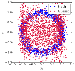
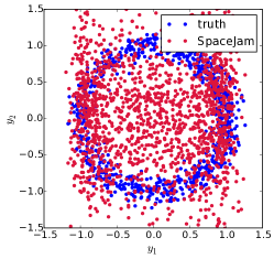
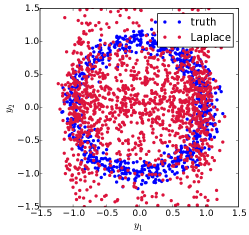
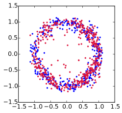
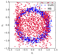
As a simple but telling example, we drew n=400𝑛400n=400 samples from a “ring” distribution in d=4𝑑4d=4 dimensions. We used m=10𝑚10m=10 expanded features and r=20𝑟20r=20 quantile levels. Data were generated by first drawing a random angle νUniform(0,1)similar-to𝜈Uniform01\nu\sim\textrm{Uniform}(0,1), then a random radius R𝒩(0,0.1)similar-to𝑅𝒩00.1R\sim\mathcal{N}(0,0.1), and finally computing the coordinates y1=Rcosνsubscript𝑦1𝑅𝜈y_{1}=R\cos\nu, y2=Rsinνsubscript𝑦2𝑅𝜈y_{2}=R\sin\nu and y3,y4𝒩(0,1)similar-tosubscript𝑦3subscript𝑦4𝒩01y_{3},y_{4}\sim\mathcal{N}(0,1), i.e., y1subscript𝑦1y_{1} and y2subscript𝑦2y_{2} are the only dependent variables here. Figure 1 plots samples (blue) of the coordinates (y1,y2)subscript𝑦1subscript𝑦2(y_{1},y_{2}) as well as new samples (red) from the MQGM, MB, GLasso, and SpaceJam fitted to these same (blue) samples; the samples from the MQGM, obtained by using our Gibbs sampler (see the supplement for further details), appear to closely match the samples from the underlying ring.
Refer to caption
Refer to caption
Refer to caption
Refer to caption
Refer to caption
Refer to caption
Figure 1: Data from the ring distribution (blue) as well as new samples (red) from the MQGM, MB, GLasso, SpaceJam, TIGER, and Laplace fitted to the same (blue) data; the samples from the MQGM were obtained by using our Gibbs sampler.

Figure 2 shows the conditional independencies recovered by the MQGM, MB, GLasso, SpaceJam, the nonparanormal skeptic, TIGER, and Laplace, when run on the ring data. We visualize these independencies by forming a d×d𝑑𝑑d\times d matrix with the cell (j,k)𝑗𝑘(j,k) set to white if j,k𝑗𝑘j,k are conditionally independent given the others, and black otherwise. Across a range of tuning parameters for each method, the MQGM is the only one that successfully recovers the underlying conditional dependencies.

Refer to caption
Refer to caption
Refer to caption
Refer to caption
Refer to caption
Refer to caption
Refer to caption
Figure 2: Conditional independencies recovered by the MQGM, MB, GLasso, SpaceJam, the nonparanormal skeptic, TIGER, and Laplace on the ring data; black means conditional dependence. The MQGM is the only method that successfully recovers the underlying conditional dependencies.

Table 6.1 presents an evaluation of the conditional CDFs given by the MQGM, MB, GLasso, SpaceJam, TIGER, and Laplace when run on the ring data. For each method, we averaged the total variation distances and Kolmogorov-Smirnoff statistics between the fitted and true conditional CDFs across all variables, and then reported the best values obtained across a range of tuning parameters (further details are given in the supplement); the MQGM outperforms all its competitors, in both metrics.

Table 1: Total variation (TV) distance and Kolmogorov-Smirnoff (KS) statistic values for the MQGM, MB, GLasso, SpaceJam, TIGER, and Laplace on the ring data; lower is better, best in bold.
TV KS
MQGM 20.873 0.760
MB 92.298 1.856
GLasso 92.479 1.768
SpaceJam 91.568 1.697
TIGER 88.284 1.450
Laplace 127.406 1.768
Larger examples

To investigate performance at larger scales, we drew n{50,100,300}𝑛50100300n\in\{50,100,300\} samples from a multivariate normal and Student t𝑡t-distribution (with 3 degrees of freedom), both in d=100𝑑100d=100 dimensions, and parameterized by a random, sparse, diagonally dominant d×d𝑑𝑑d\times d inverse covariance matrix, following the procedure in Peng et al. (2009); Khare et al. (2014); Oh et al. (2014); Ali et al. (2016). Over the same set of sample sizes, with d=100𝑑100d=100, we also considered an autoregressive setup in which we drew samples of pairs of adjacent variables from the ring distribution. In all three data settings (normal, t𝑡t, and autoregressive), we used m=10𝑚10m=10 and r=20𝑟20r=20 for the MQGM. To summarize the performances, we considered a range of tuning parameters for each method, computed corresponding false and true positive rates (in detecting conditional dependencies), and then computed the corresponding area under the curve (AUC), following, e.g., Peng et al. (2009); Khare et al. (2014); Oh et al. (2014); Ali et al. (2016). Table 6.1 reports the median AUCs (across 50 trials) for all three of these examples; the MQGM outperforms all other methods on the autoregressive example, as well as on the small-n𝑛n normal and Student t𝑡t examples.

Table 2: AUC values for the MQGM, MB, GLasso, SpaceJam, the nonparanormal skeptic, TIGER, and Laplace for the normal, t𝑡t, and autoregressive data settings; higher is better, best in bold (standard errors are 104absentsuperscript104\approx 10^{-4} or smaller).

6.2 Modeling flu epidemics

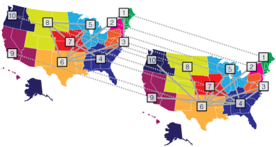
We study n=937𝑛937n=937 weekly flu incidence reports from September 28, 1997 through August 30, 2015, across 10 regions in the United States (see the left panel of Figure 3), obtained from Centers for Disease Control and Prevention (2015) (CDC). We considered d=20𝑑20d=20 variables: the first 10 encode the current week’s flu incidence (precisely, the percentage of doctor’s visits in which flu-like symptoms are presented) in the 10 regions, and the last 10 encode the same but for the prior week. We set m=5𝑚5m=5, r=99𝑟99r=99, and also introduced exogenous variables to encode the week numbers, so p=1𝑝1p=1. Thus, learning the MQGM here corresponds to learning the structure of a spatiotemporal graphical model, and reduces to solving 20 multiple quantile regression subproblems, each of dimension (19×5+1)×99=95041951999504(19\times 5+1)\times 99=9504. All subproblems took about 1 minute on a 6 core 3.3 Ghz Core i7 X980 processor.

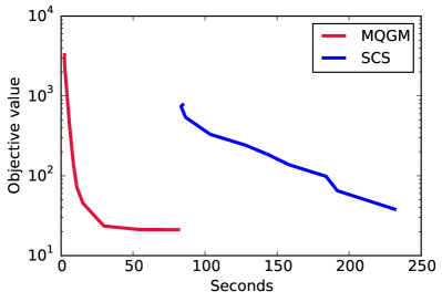
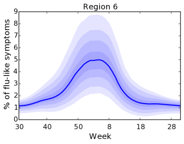
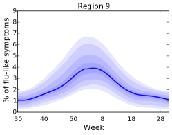
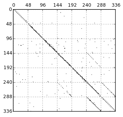
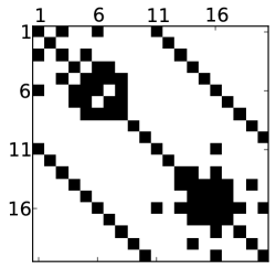
The left panel of Figure 4 plots the wallclock time (seconds) for solving one subproblem using ADMM versus SCS (O’Donoghue et al., 2013), a cone solver that has been advocated as a reasonable choice for a class of problems encapsulating (4); ADMM outperforms SCS by roughly two orders of magnitude. The right panel of Figure 3 presents the conditional independencies recovered by the MQGM. Nonzero entries in the upper left 10×10101010\times 10 submatrix correspond to dependencies between the yksubscript𝑦𝑘y_{k} variables for k=1,,10𝑘110k=1,\ldots,10; e.g., the nonzero (0,2) entry suggests that region 1 and 3’s flu reports are dependent. The lower right 10×10101010\times 10 submatrix corresponds to the yksubscript𝑦𝑘y_{k} variables for k=11,,20𝑘1120k=11,\ldots,20, and the nonzero banded entries suggest that at any region the previous week’s flu incidence (naturally) influences the next week’s. The left panel of Figure 3 visualizes these relationships by drawing an edge between dependent regions; region 6 is highly connected, suggesting that it is a bellwether for other regions, which is a qualitative observation also made by the CDC. To draw samples from the fitted distributions, we ran our Gibbs sampler over the year, generating 1000 total samples, making 5 passes over all coordinates between each sample, and with a burn-in period of 100 iterations. The right panel of Figure 4 plots samples from the marginal distribution of the percentages of flu reports at region six (other regions are in the supplement) throughout the year, revealing the heteroskedastic nature of the data; we also see that flu incidence (naturally) increases towards the end of the year.
Refer to caption
Refer to caption
Figure 3: Conditional dependencies recovered by the MQGM on the flu data; each of the first ten cells on the right corresponds to a region of the U.S. on the left, and black means dependence.
Refer to caption
Refer to caption
Figure 4: Wallclock time (seconds) for solving one subproblem using ADMM versus SCS, on the left. Samples from the fitted marginal distribution of the weekly flu incidence rates at region six, on the right. Samples at larger quantiles are shaded lighter; the median is in darker blue.

Our last example, on wind power data, is presented in the supplement.

7 Discussion

We proposed and studied the Multiple Quantile Graphical Model (MQGM). We established theoretical and empirical backing to the claim that the MQGM is capable of compactly representing relationships between heteroskedastic, non-Gaussian variables. We developed efficient algorithms for estimation and sampling in the MQGM. All in all, we believe that our work represents a step forward in the design of flexible yet tractable graphical models.

Acknowledgments

This work was supported by a Department of Energy Computational Science Graduate Fellowship, under grant number DE-FG02-97ER25308.

References

  • Ali et al. (2016) Alnur Ali, Kshitij Khare, Sang-Yun Oh, and Bala Rajaratnam. Generalized pseudolikelihood methods for inverse covariance estimation. Technical report, 2016. Available at http://arxiv.org/pdf/1606.00033.pdf.
  • Banerjee et al. (2008) Onureena Banerjee, Laurent El Ghaoui, and Alexandre d’Aspremont. Model selection through sparse maximum likelihood estimation for multivariate Gaussian or binary data. Journal of Machine Learning Research, 9:485–516, 2008.
  • Belloni and Chernozhukov (2011) Alexandre Belloni and Victor Chernozhukov. 1subscript1\ell_{1}-penalized quantile regression in high-dimensional sparse models. Annals of Statistics, 39(1):82–130, 2011.
  • Besag (1974) Julian Besag. Spatial interaction and the statistical analysis of lattice systems. Journal of the Royal Statistical Society: Series B, 36(2):192–236, 1974.
  • Bishop (2006) Christopher Bishop. Pattern Recognition and Machine Learning. Springer, 2006.
  • Boyd et al. (2011) Stephen Boyd, Neal Parikh, Eric Chu, Borja Peleato, and Jonathan Eckstein. Distributed optimization and statistical learning via the alternating direction method of multipliers. Foundations and Trends in Machine Learning, 3(1):1–122, 2011.
  • Centers for Disease Control and Prevention (2015) (CDC) Centers for Disease Control and Prevention (CDC). Influenza national and regional level graphs and data, August 2015. URL http://gis.cdc.gov/grasp/fluview/fluportaldashboard.html.
  • Chen et al. (2015) Shizhe Chen, Daniela Witten, and Ali Shojaie. Selection and estimation for mixed graphical models. Biometrika, 102(1):47–64, 2015.
  • Dempster (1972) Arthur Dempster. Covariance selection. Biometrics, 28(1):157–175, 1972.
  • Fan et al. (2014) Jianqing Fan, Yingying Fan, and Emre Barut. Adaptive robust variable selection. Annals of Statistics, 42(1):324–351, 2014.
  • Finegold and Drton (2011) Michael Finegold and Mathias Drton. Robust graphical modeling of gene networks using classical and alternative t-distributions. Annals of Applied Statistics, 5(2A):1057–1080, 2011.
  • Friedman et al. (2008) Jerome Friedman, Trevor Hastie, and Robert Tibshirani. Sparse inverse covariance estimation with the graphical lasso. Biostatistics, 9(3):432–441, 2008.
  • Friedman et al. (2010) Jerome Friedman, Trevor Hastie, and Robert Tibshirani. Applications of the lasso and grouped lasso to the estimation of sparse graphical models. Technical report, 2010. Available at http://statweb.stanford.edu/~tibs/ftp/ggraph.pdf.
  • Gyrofi et al. (2002) Laszlo Gyrofi, Michael Kohler, Adam Krzyzak, and Harro Walk. A Distribution-Free Theory of Nonparametric Regression. 2002.
  • Heckerman et al. (2000) David Heckerman, David Maxwell Chickering, David Meek, Robert Rounthwaite, and Carl Kadie. Dependency networks for inference, collaborative filtering, and data visualization. Journal of Machine Learning Research, 1:49–75, 2000.
  • Höfling and Tibshirani (2009) Holger Höfling and Robert Tibshirani. Estimation of sparse binary pairwise Markov networks using pseudo-likelihoods. Journal of Machine Learning Research, 10:883–906, 2009.
  • Hong et al. (2014) Tao Hong, Pierre Pinson, and Shu Fan. Global energy forecasting competition 2012. International Journal of Forecasting, 30:357–363, 2014.
  • Johnson (2013) Nicholas Johnson. A dynamic programming algorithm for the fused lasso and 0subscript0\ell_{0}-segmentation. Journal of Computational and Graphical Statistics, 22(2):246–260, 2013.
  • Kato (2011) Kengo Kato. Group lasso for high dimensional sparse quantile regression models. Technical report, 2011. Available at http://arxiv.org/pdf/1103.1458.pdf.
  • Khare et al. (2014) Kshitij Khare, Sang-Yun Oh, and Bala Rajaratnam. A convex pseudolikelihood framework for high dimensional partial correlation estimation with convergence guarantees. Journal of the Royal Statistical Society: Series B, 77(4):803–825, 2014.
  • Koenker (2005) Roger Koenker. Quantile Regression. Cambridge University Press, 2005.
  • Koenker (2011) Roger Koenker. Additive models for quantile regression: Model selection and confidence bandaids. Brazilian Journal of Probability and Statistics, 25(3):239–262, 2011.
  • Koenker and Bassett (1978) Roger Koenker and Gilbert Bassett. Regression quantiles. Econometrica, 46(1):33–50, 1978.
  • Koenker et al. (1994) Roger Koenker, Pin Ng, and Stephen Portnoy. Quantile smoothing splines. Biometrika, 81(4):673–680, 1994.
  • Lauritzen (1996) Steffen Lauritzen. Graphical models. Oxford University Press, 1996.
  • Lee and Hastie (2013) Jason Lee and Trevor Hastie. Structure learning of mixed graphical models. In Proceedings of the 16th International Conference on Artificial Intelligence and Statistics, pages 388–396, 2013.
  • Liu and Wang (2012) Han Liu and Lie Wang. TIGER: A tuning-insensitive approach for optimally estimating Gaussian graphical models. Technical report, 2012. Available at http://arxiv.org/pdf/1209.2437.pdf.
  • Liu et al. (2009) Han Liu, John Lafferty, and Larry Wasserman. The nonparanormal: Semiparametric estimation of high dimensional undirected graphs. Journal of Machine Learning Research, 10:2295–2328, 2009.
  • Liu et al. (2012) Han Liu, Fang Han, Ming Yuan, John Lafferty, and Larry Wasserman. High-dimensional semiparametric Gaussian copula graphical models. The Annals of Statistics, pages 2293–2326, 2012.
  • Meier et al. (2009) Lukas Meier, Sara van de Geer, and Peter Buhlmann. High-dimensional additive modeling. Annals of Statistics, 37(6):3779–3821, 2009.
  • Meinshausen and Bühlmann (2006) Nicolai Meinshausen and Peter Bühlmann. High-dimensional graphs and variable selection with the lasso. Annals of Statistics, 34(3):1436–1462, 2006.
  • Neville and Jensen (2004) Jennifer Neville and David Jensen. Dependency networks for relational data. In Proceedings of Fourth IEEE International Conference on the Data Mining, pages 170–177. IEEE, 2004.
  • O’Donoghue et al. (2013) Brendan O’Donoghue, Eric Chu, Neal Parikh, and Stephen Boyd. Operator splitting for conic optimization via homogeneous self-dual embedding. Technical report, 2013. Available at https://stanford.edu/~boyd/papers/pdf/scs.pdf.
  • Oh et al. (2014) Sang-Yun Oh, Onkar Dalal, Kshitij Khare, and Bala Rajaratnam. Optimization methods for sparse pseudolikelihood graphical model selection. In Advances in Neural Information Processing Systems 27, pages 667–675, 2014.
  • Parikh and Boyd (2013) Neal Parikh and Stephen Boyd. Proximal algorithms. Foundations and Trends in Optimization, 1(3):123–231, 2013.
  • Peng et al. (2009) Jie Peng, Pei Wang, Nengfeng Zhou, and Ji Zhu. Partial correlation estimation by joint sparse regression models. Journal of the American Statistical Association, 104(486):735–746, 2009.
  • Raskutti et al. (2012) Garvesh Raskutti, Martin Wainwright, and Bin Yu. Minimax-optimal rates for sparse additive models over kernel classes via convex programming. Journal of Machine Learning Research, 13:389–427, 2012.
  • Rocha et al. (2008) Guilherme Rocha, Peng Zhao, and Bin Yu. A path following algorithm for sparse pseudo-likelihood inverse covariance estimation (SPLICE). Technical report, 2008. Available at https://www.stat.berkeley.edu/~binyu/ps/rocha.pseudo.pdf.
  • Rothman et al. (2008) Adam Rothman, Peter Bickel, Elizaveta Levina, and Ji Zhu. Sparse permutation invariant covariance estimation. Electronic Journal of Statistics, 2:494–515, 2008.
  • Sohn and Kim (2012) Kyung-Ah Sohn and Seyoung Kim. Joint estimation of structured sparsity and output structure in multiple-output regression via inverse covariance regularization. In Proceedings of the 15th International Conference on Artificial Intelligence and Statistics, pages 1081–1089, 2012.
  • Takeuchi et al. (2006) Ichiro Takeuchi, Quoc Le, Timothy Sears, and Alexander Smola. Nonparametric quantile estimation. Journal of Machine Learning Research, 7:1231–1264, 2006.
  • Varin and Vidoni (2005) Cristiano Varin and Paolo Vidoni. A note on composite likelihood inference and model selection. Biometrika, 92(3):519–528, 2005.
  • Voorman et al. (2014) Arend Voorman, Ali Shojaie, and Daniela Witten. Graph estimation with joint additive models. Biometrika, 101(1):85–101, 2014.
  • Wainwright (2009) Martin Wainwright. Sharp thresholds for high-dimensional and noisy sparsity recovery using-constrained quadratic programming (Lasso). IEEE Transactions on Information Theory, 55(5):2183–2202, 2009.
  • Wang and Ip (2008) Yuchung Wang and Edward Ip. Conditionally specified continuous distributions. Biometrika, 95(3):735–746, 2008.
  • Wytock and Kolter (2013) Matt Wytock and Zico Kolter. Sparse Gaussian conditional random fields: Algorithms, theory, and application to energy forecasting. In Proceedings of the 30th International Conference on Machine Learning, pages 1265–1273, 2013.
  • Yang et al. (2012) Eunho Yang, Pradeep Ravikumar, Genevera Allen, and Zhandong Liu. Graphical models via generalized linear models. In Advances in Neural Information Processing Systems 25, pages 1358–1366, 2012.
  • Yang et al. (2015) Eunho Yang, Pradeep Ravikumar, Genevera Allen, and Zhandong Liu. Graphical models via univariate exponential family distributions. Journal of Machine Learning Research, 16:3813–3847, 2015.
  • Yuan and Lin (2007) Ming Yuan and Yi Lin. Model selection and estimation in the Gaussian graphical model. Biometrika, 94(1):19–35, 2007.
  • Yuan and Zhang (2014) Xiao-Tong Yuan and Tong Zhang. Partial Gaussian graphical model estimation. IEEE Transactions on Information Theory, 60(3):1673–1687, 2014.

Supplement to “The Multiple Quantile Graphical Model”

S.1 Proof of Lemma 4.1

If the conditional quantiles satisfy QU|V,W(α)=QU|W(α)subscript𝑄conditional𝑈𝑉𝑊𝛼subscript𝑄conditional𝑈𝑊𝛼Q_{U|V,W}(\alpha)=Q_{U|W}(\alpha) for all α[0,1]𝛼01\alpha\in[0,1], then the conditional CDF must obey the same property, i.e., FU|V,W(t)=FU|W(t)subscript𝐹conditional𝑈𝑉𝑊𝑡subscript𝐹conditional𝑈𝑊𝑡F_{U|V,W}(t)=F_{U|W}(t) for all t𝑡t in the support of U𝑈U. This is simply because any CDF may be expressed in terms of its corresponding quantile function (i.e., inverse CDF), as in

FU|V,W(t)=sup{α[0,1]:QU|V,W(α)t},subscript𝐹conditional𝑈𝑉𝑊𝑡supremumconditional-set𝛼01subscript𝑄conditional𝑈𝑉𝑊𝛼𝑡F_{U|V,W}(t)=\sup\{\alpha\in[0,1]:Q_{U|V,W}(\alpha)\leq t\},

and the right-hand side does not depend on V𝑉V, so neither can the left-hand side. But this precisely implies that the distribution of U|V,Wconditional𝑈𝑉𝑊U|V,W equals that of U|Wconditional𝑈𝑊U|W, i.e., U𝑈U and V𝑉V are conditionally independent given W𝑊W. We note that the converse of the statement in the lemma is true as well, by just reversing all the arguments here. ∎

S.2 Proof of Lemma 4.2

This result can be seen as a generalization of Theorem 3 in Heckerman et al. (2000).

First, we define an iteration of Gibbs sampling to be a single pass through all the variables (without a loss of generality, we take this order to be y1,,ydsubscript𝑦1subscript𝑦𝑑y_{1},\ldots,y_{d}). Now, consider a particular iteration of Gibbs sampling; let y~1,,y~dsubscript~𝑦1subscript~𝑦𝑑\tilde{y}_{1},\ldots,\tilde{y}_{d} be the values assigned to the variables on the previous iteration. Then the transition kernel for our Gibbs sampler is given by

𝐏𝐫(y1,,yd|y~1,,y~d)𝐏𝐫subscript𝑦1conditionalsubscript𝑦𝑑subscript~𝑦1subscript~𝑦𝑑\displaystyle\mathop{\bf Pr}(y_{1},\ldots,y_{d}|\tilde{y}_{1},\ldots,\tilde{y}_{d}) =𝐏𝐫(yd|yd1,,y1,y~1,,y~d)𝐏𝐫(yd1,,y1|y~1,,y~d)absent𝐏𝐫conditionalsubscript𝑦𝑑subscript𝑦𝑑1subscript𝑦1subscript~𝑦1subscript~𝑦𝑑𝐏𝐫subscript𝑦𝑑1conditionalsubscript𝑦1subscript~𝑦1subscript~𝑦𝑑\displaystyle=\mathop{\bf Pr}(y_{d}|y_{d-1},\ldots,y_{1},\tilde{y}_{1},\ldots,\tilde{y}_{d})\mathop{\bf Pr}(y_{d-1},\ldots,y_{1}|\tilde{y}_{1},\ldots,\tilde{y}_{d}) (S.1)
=𝐏𝐫(yd|yd1,,y1)𝐏𝐫(yd1,,y1|y~1,,y~d)absent𝐏𝐫conditionalsubscript𝑦𝑑subscript𝑦𝑑1subscript𝑦1𝐏𝐫subscript𝑦𝑑1conditionalsubscript𝑦1subscript~𝑦1subscript~𝑦𝑑\displaystyle=\mathop{\bf Pr}(y_{d}|y_{d-1},\ldots,y_{1})\mathop{\bf Pr}(y_{d-1},\ldots,y_{1}|\tilde{y}_{1},\ldots,\tilde{y}_{d}) (S.2)
=𝐏𝐫(yd|yd1,,y1)𝐏𝐫(yd1|yd2,y1,y~d)𝐏𝐫(y1|y~2,,y~d),absent𝐏𝐫conditionalsubscript𝑦𝑑subscript𝑦𝑑1subscript𝑦1𝐏𝐫conditionalsubscript𝑦𝑑1subscript𝑦𝑑2subscript𝑦1subscript~𝑦𝑑𝐏𝐫conditionalsubscript𝑦1subscript~𝑦2subscript~𝑦𝑑\displaystyle=\mathop{\bf Pr}(y_{d}|y_{d-1},\ldots,y_{1})\mathop{\bf Pr}(y_{d-1}|y_{d-2},\ldots y_{1},\tilde{y}_{d})\cdots\mathop{\bf Pr}(y_{1}|\tilde{y}_{2},\ldots,\tilde{y}_{d}), (S.3)

where (S.1) follows by the definition of conditional probability, (S.2) by conditional independence, and (S.3) by repeated applications of these tools. Since each conditional distribution is assumed to be (strictly) positive, we have that the transition kernel is also positive, which in turn implies (Bishop, 2006, page 544) that the induced Markov chain is ergodic with a unique stationary distribution that can be reached from any initial point. ∎

S.3 Statement and discussion of regularity conditions for Theorem 4.3

For each k=1,,r𝑘1𝑟k=1,\ldots,r, =1,,r1𝑟\ell=1,\ldots,r, let us define the “effective” (independent) error terms ϵki=yk(i)bkjkϕ(yj(i))Tθkjsubscriptitalic-ϵ𝑘𝑖superscriptsubscript𝑦𝑘𝑖superscriptsubscript𝑏𝑘subscript𝑗𝑘italic-ϕsuperscriptsuperscriptsubscript𝑦𝑗𝑖𝑇superscriptsubscript𝜃𝑘𝑗\epsilon_{\ell ki}=y_{k}^{(i)}-b_{\ell k}^{*}-\sum_{j\neq k}\phi(y_{j}^{(i)})^{T}\theta_{\ell kj}^{*}, over i=1,,n𝑖1𝑛i=1,\ldots,n. Denote by Fϵksubscript𝐹subscriptitalic-ϵ𝑘F_{\epsilon_{\ell k}} the conditional CDF of ϵki|y¬k(i)conditionalsubscriptitalic-ϵ𝑘𝑖superscriptsubscript𝑦𝑘𝑖\epsilon_{\ell ki}|y_{\neg k}^{(i)}, i=1,,n𝑖1𝑛i=1,\ldots,n, which by construction satisfies Fϵk(0)=αsubscript𝐹subscriptitalic-ϵ𝑘0subscript𝛼F_{\epsilon_{\ell k}}(0)=\alpha_{\ell}. Also define the underlying support

Sk={j{1,,d}:θkj0}.subscript𝑆𝑘conditional-set𝑗1𝑑superscriptsubscript𝜃𝑘𝑗0S_{\ell k}=\big{\{}j\in\{1,\ldots,d\}:\theta_{\ell kj}^{*}\not=0\big{\}}.

Here we take a moment to explain a somewhat subtle indexing issue with the columns of the feature matrix ΦRn×dmΦsuperscriptR𝑛𝑑𝑚\Phi\in{\mbox{\bf R}}^{n\times dm}. For a single fixed index j=1,,d𝑗1𝑑j=1,\ldots,d, we will extract an appropriate block of columns of ΦRn×dmΦsuperscriptR𝑛𝑑𝑚\Phi\in{\mbox{\bf R}}^{n\times dm}, corresponding to the basis expansion of variable j𝑗j, by writing ΦjsubscriptΦ𝑗\Phi_{j}. More precisely, we use ΦjsubscriptΦ𝑗\Phi_{j} to denote the block of m𝑚m columns

[Φ(j1)m+1,Φ(j1)m+2,,Φjm].subscriptΦ𝑗1𝑚1subscriptΦ𝑗1𝑚2subscriptΦ𝑗𝑚[\Phi_{(j-1)m+1},\Phi_{(j-1)m+2},\ldots,\Phi_{jm}]. (S.4)

We do this because it simplifies notation considerably. (Occasionally, to be transparent, we will use the more exhaustive notation on the right-hand side in (S.4), but this is to be treated as an exception, and the default is to use the concise notation as in ΦjsubscriptΦ𝑗\Phi_{j}.) The same rule will be used for subsets of indices among 1,,d1𝑑1,\ldots,d, so that ΦSksubscriptΦsubscript𝑆𝑘\Phi_{S_{\ell k}} denotes the appropriate block of m|Sk|𝑚subscript𝑆𝑘m|S_{\ell k}| columns corresponding to the basis expansions of the variables in Sksubscript𝑆𝑘S_{\ell k}.

For all k=1,,d𝑘1𝑑k=1,\ldots,d, =1,,r1𝑟\ell=1,\ldots,r, we will assume the following regularity conditions.

  1. A1.

    Groupwise irrepresentability: for jSkc𝑗superscriptsubscript𝑆𝑘𝑐j\in S_{\ell k}^{c}, we require that ΦjTΦSkF<λ1/(6fϵk(0)γ)subscriptnormsuperscriptsubscriptΦ𝑗𝑇subscriptΦsubscript𝑆𝑘𝐹subscript𝜆16subscript𝑓subscriptitalic-ϵ𝑘0𝛾\|\Phi_{j}^{T}\Phi_{S_{\ell k}}\|_{F}<\lambda_{1}/(6f_{\epsilon_{\ell k}}(0)\gamma), where Sk={j{1,,dm}:θkj0}subscript𝑆𝑘conditional-set𝑗1𝑑𝑚superscriptsubscript𝜃𝑘𝑗0S_{\ell k}=\{j\in\{1,\ldots,dm\}:\theta_{\ell kj}^{*}\neq 0\}, fϵksubscript𝑓subscriptitalic-ϵ𝑘f_{\epsilon_{\ell k}} is the density of Fϵksubscript𝐹subscriptitalic-ϵ𝑘F_{\epsilon_{\ell k}}, and γ>0𝛾0\gamma>0 is a quantity prescribed by Lemma S.5.

  2. A2.

    Distributional smoothness: we assume that |Fϵk(x)Fϵk(0)xfϵk(0)|C1x2subscript𝐹subscriptitalic-ϵ𝑘𝑥subscript𝐹subscriptitalic-ϵ𝑘0𝑥subscript𝑓subscriptitalic-ϵ𝑘0subscript𝐶1superscript𝑥2|F_{\epsilon_{\ell k}}(x)-F_{\epsilon_{\ell k}}(0)-xf_{\epsilon_{\ell k}}(0)|\leq C_{1}x^{2} for all |x|C2𝑥subscript𝐶2|x|\leq C_{2}, where C1,C2>0subscript𝐶1subscript𝐶20C_{1},C_{2}>0 are constants.

  3. A3.

    Correlation restriction: we assume that C3(fϵk(0)/n)λmin(ΦSkTΦSk)C4subscript𝐶3subscript𝑓subscriptitalic-ϵ𝑘0𝑛subscript𝜆superscriptsubscriptΦsubscript𝑆𝑘𝑇subscriptΦsubscript𝑆𝑘subscript𝐶4C_{3}\leq(f_{\epsilon_{\ell k}}(0)/n)\lambda_{\min}(\Phi_{S_{\ell k}}^{T}\Phi_{S_{\ell k}})\leq C_{4} for constants C3,C4>0subscript𝐶3subscript𝐶40C_{3},C_{4}>0, where λmin(A)subscript𝜆𝐴\lambda_{\min}(A) denotes the minimum eigenvalue of A𝐴A.

  4. A4.

    Basis and support size restrictions: we assume that m=O(n1/9)𝑚𝑂superscript𝑛19m=O(n^{1/9}) and s=O(n1/21)𝑠𝑂superscript𝑛121s=O(n^{1/21}), where s=|Sk|𝑠subscript𝑆𝑘s=|S_{\ell k}|. We also assume, with probability tending to one, that Φmax=Ω(1)subscriptΦΩ1\Phi_{\max}=\Omega(1) and Φmax=o(n1/21/log1/2n)subscriptΦ𝑜superscript𝑛121superscript12𝑛\Phi_{\max}=o(n^{1/21}/\log^{1/2}n), where we write ΦmaxsubscriptΦ\Phi_{\max} to denote the maximum absolute entry of the basis matrix ΦΦ\Phi.

Next, we provide some intuition for these conditions.


Condition A1. Fix some jSkc𝑗superscriptsubscript𝑆𝑘𝑐j\in S_{\ell k}^{c}. For notational convenience, we let

A=ΦjTΦSkRm×sm.𝐴superscriptsubscriptΦ𝑗𝑇subscriptΦsubscript𝑆𝑘superscriptR𝑚𝑠𝑚A=\Phi_{j}^{T}\Phi_{S_{\ell k}}\in{\mbox{\bf R}}^{m\times sm}.

Observe that each entry of A𝐴A can be expressed as

Aip=nρi,pΦ(j1)m+i2Φp2,subscript𝐴𝑖𝑝𝑛subscript𝜌𝑖𝑝subscriptnormsubscriptΦ𝑗1𝑚𝑖2subscriptnormsubscriptΦ𝑝2A_{ip}=n\rho_{i,p}\|\Phi_{(j-1)m+i}\|_{2}\|\Phi_{p}\|_{2}, (S.5)

for i=1,,m𝑖1𝑚i=1,\ldots,m, p𝑝p denoting an index into the basis expansion of the columns ΦSksubscriptΦsubscript𝑆𝑘\Phi_{S_{\ell k}}, and ρi,psubscript𝜌𝑖𝑝\rho_{i,p} denoting the sample correlation coefficient for the columns ΦisubscriptΦ𝑖\Phi_{i} and ΦpsubscriptΦ𝑝\Phi_{p}. Since ApFmApsubscriptnormsubscript𝐴𝑝𝐹𝑚subscriptnormsubscript𝐴𝑝\|A_{p}\|_{F}\leq\sqrt{m}\|A_{p}\|_{\infty}, we have that

maxi,pρi,p<λ16n2fϵk(0)msubscript𝑖𝑝subscript𝜌𝑖𝑝subscript𝜆16superscript𝑛2subscript𝑓subscriptitalic-ϵ𝑘0𝑚\max_{i,p}\;\rho_{i,p}<\frac{\lambda_{1}}{6n^{2}f_{\epsilon_{\ell k}}(0)\sqrt{m}}

is sufficient for condition A1; here, we have also used the column scaling assumption Φp2nsubscriptnormsubscriptΦ𝑝2𝑛\|\Phi_{p}\|_{2}\leq\sqrt{n}.

So, roughly speaking, bounded correlation between each pair of columns in the submatrices ΦjsubscriptΦ𝑗\Phi_{j} and ΦSksubscriptΦsubscript𝑆𝑘\Phi_{S_{\ell k}} is enough for condition A1 to hold; note that this is trivially satisfied when ΦiTΦp=0superscriptsubscriptΦ𝑖𝑇subscriptΦ𝑝0\Phi_{i}^{T}\Phi_{p}=0, for i=1,,m𝑖1𝑚i=1,\ldots,m, and p𝑝p as defined above. Condition A1 is therefore similar to, e.g., the mutual incoherence condition of Wainwright (2009) for the lasso, which is given by

ΦScTΦS(ΦSTΦS)11γ~maxjSc(ΦSTΦS)1ΦSTΦj11γ~,iffsubscriptnormsuperscriptsubscriptΦsuperscript𝑆𝑐𝑇subscriptΦ𝑆superscriptsuperscriptsubscriptΦ𝑆𝑇subscriptΦ𝑆11~𝛾subscript𝑗superscript𝑆𝑐subscriptnormsuperscriptsuperscriptsubscriptΦ𝑆𝑇subscriptΦ𝑆1superscriptsubscriptΦ𝑆𝑇subscriptΦ𝑗11~𝛾\displaystyle\left\|\Phi_{S^{c}}^{T}\Phi_{S}\left(\Phi_{S}^{T}\Phi_{S}\right)^{-1}\right\|_{\infty}\leq 1-\tilde{\gamma}\iff\max_{j\in S^{c}}\left\|\left(\Phi_{S}^{T}\Phi_{S}\right)^{-1}\Phi_{S}^{T}\Phi_{j}\right\|_{1}\leq 1-\tilde{\gamma},

where again ΦSsubscriptΦ𝑆\Phi_{S} extracts the appropriate block of columns of ΦΦ\Phi, \|\cdot\|_{\infty} here denotes the subscript\ell_{\infty} operator norm (maximum 1subscript1\ell_{1} norm of a row), 1\|\cdot\|_{1} here denotes the elementwise 1subscript1\ell_{1} norm, and γ~(0,1]~𝛾01\tilde{\gamma}\in(0,1] is a constant. This condition can be seen as requiring bounded correlation between each column in the submatrix ΦScsubscriptΦsuperscript𝑆𝑐\Phi_{S^{c}} and all columns in the submatrix ΦSsubscriptΦ𝑆\Phi_{S}.


Condition A2. This condition is similar to requiring that fϵk(x)subscript𝑓subscriptitalic-ϵ𝑘𝑥f_{\epsilon_{\ell k}}(x) be Lipschitz, over some x𝑥x in a neighborhood of 0. We can show that the Laplace distribution, e.g., satisfies this condition.

The density and distribution functions for the Laplace distribution with location zero and unit scale are given by

fϵk(x)=(1/2)exp(|x|)subscript𝑓subscriptitalic-ϵ𝑘𝑥12𝑥f_{\epsilon_{\ell k}}(x)=(1/2)\exp(-|x|)

and

Fϵk(x)={1(1/2)exp(x)if x0(1/2)exp(x)if x<0,subscript𝐹subscriptitalic-ϵ𝑘𝑥cases112𝑥if 𝑥012𝑥if 𝑥0F_{\epsilon_{\ell k}}(x)=\begin{cases}1-(1/2)\exp(-x)&\textrm{if }x\geq 0\\ (1/2)\exp(x)&\textrm{if }x<0,\end{cases}

respectively.

Now, suppose 0xC20𝑥subscript𝐶20\leq x\leq C_{2}. Then we can express condition A2 as

|fϵk(x)fϵk(0)xfϵk(0)|C1x22C1x2exp(x)+x12C1x2.iffsubscript𝑓subscriptitalic-ϵ𝑘𝑥subscript𝑓subscriptitalic-ϵ𝑘0𝑥subscript𝑓subscriptitalic-ϵ𝑘0subscript𝐶1superscript𝑥22subscript𝐶1superscript𝑥2𝑥𝑥12subscript𝐶1superscript𝑥2\displaystyle|f_{\epsilon_{\ell k}}(x)-f_{\epsilon_{\ell k}}(0)-xf_{\epsilon_{\ell k}}(0)|\leq C_{1}x^{2}\iff-2C_{1}x^{2}\leq\exp(-x)+x-1\leq 2C_{1}x^{2}.

For the first inequality, since 1xexp(x)1𝑥𝑥1-x\leq\exp(-x), it is sufficient to check that 0C1x20subscript𝐶1superscript𝑥20\leq C_{1}x^{2}, which is true for C1>0subscript𝐶10C_{1}>0 and all x𝑥x. For the second inequality, by differentiating and again using 1xexp(x)1𝑥𝑥1-x\leq\exp(-x), we have that the function

2C1x2exp(x)x+12subscript𝐶1superscript𝑥2𝑥𝑥12C_{1}x^{2}-\exp(-x)-x+1 (S.6)

is nondecreasing in x0𝑥0x\geq 0; thus, it is sufficient to check that this function is nonnegative for x=0𝑥0x=0, which is true.

Now, suppose C2x<0subscript𝐶2𝑥0-C_{2}\leq x<0. Then we can express condition A2 as

|fϵk(x)fϵk(0)xfϵk(0)|C1x22C1x2exp(x)x12C1x2.iffsubscript𝑓subscriptitalic-ϵ𝑘𝑥subscript𝑓subscriptitalic-ϵ𝑘0𝑥subscript𝑓subscriptitalic-ϵ𝑘0subscript𝐶1superscript𝑥22subscript𝐶1superscript𝑥2𝑥𝑥12subscript𝐶1superscript𝑥2\displaystyle|f_{\epsilon_{\ell k}}(x)-f_{\epsilon_{\ell k}}(0)-xf_{\epsilon_{\ell k}}(0)|\leq C_{1}x^{2}\iff-2C_{1}x^{2}\leq\exp(x)-x-1\leq 2C_{1}x^{2}.

By symmetry with the preceding case, the first inequality here holds. The second inequality here also holds, since exp(x)2C1x2x1𝑥2subscript𝐶1superscript𝑥2𝑥1\exp(x)-2C_{1}x^{2}-x-1 is continuous and increasing in x<0𝑥0x<0; taking the limit as x0𝑥0x\uparrow 0 gives that this function is nonpositive as required.


Condition A3. This condition is a generalization of the minimum eigenvalue condition of Wainwright (2009), i.e., cminλmin((1/n)ΦSTΦS),subscript𝑐subscript𝜆1𝑛superscriptsubscriptΦ𝑆𝑇subscriptΦ𝑆c_{\min}\leq\lambda_{\min}\left((1/n)\Phi_{S}^{T}\Phi_{S}\right), for some constant cmin>0subscript𝑐0c_{\min}>0, and where we write ΦSsubscriptΦ𝑆\Phi_{S} to extract the appropriate block of columns of ΦΦ\Phi.


Condition A4. This condition allows the number of basis functions m𝑚m in the expansion to grow with n𝑛n, at a polynomial rate (with fractional exponent). This is roughly in line with standard nonparametric regression; e.g., when estimating a continuous differentiable function via a spline expansion, one typically takes the number of basis functions m𝑚m to scale as n1/3superscript𝑛13n^{1/3}, and the more derivatives that are assumed, the smaller the fractional exponent (Gyrofi et al., 2002). The condition also restricts, for any given variable, the number of variables s𝑠s that contribute to its neighborhood model to be polynomial in n𝑛n (with a smaller fractional exponent).

Finally, the condition assumes that the entries of the basis matrix ΦΦ\Phi (i.e., the matrix of transformed variables) to be at least of constant order, and at most of polynomial order (with small fractional exponent), with n𝑛n. We note that this implicitly places a restriction on the tails of distribution governing the data yj(i)subscriptsuperscript𝑦𝑖𝑗y^{(i)}_{j}, i=1,,n𝑖1𝑛i=1,\ldots,n, j=1,,d𝑗1𝑑j=1,\ldots,d. However, the restriction is not a strong one, because it allows the maximum to grow polynomially large with n𝑛n (whereas a logarithmic growth would be expected, e.g., for normal data). Furthermore, it is possible to trade off the restrictions on m𝑚m, s𝑠s, ΦmaxsubscriptΦ\Phi_{\max}, and d𝑑d (presented in the statement of the theorem), making each of these restrictions more or less stringent, if required.

S.4 Proof of Theorem 4.3

The general strategy that we use here for support recovery is inspired by that in Fan et al. (2014), for 1subscript1\ell_{1}-penalized quantile regression.

Fix some k=1,,d𝑘1𝑑k=1,\ldots,d and =1,,r1𝑟\ell=1,\ldots,r. We consider the conditional distribution yk|y¬kconditionalsubscript𝑦𝑘subscript𝑦𝑘y_{k}|y_{\neg k}, whose αsubscript𝛼\alpha_{\ell}-quantile is assumed to satisfy (3). Hence, to be perfectly clear, all expectations and probability statements in what follows are to be interpreted with respect to the observations yk(i)superscriptsubscript𝑦𝑘𝑖y_{k}^{(i)}, i=1,,n𝑖1𝑛i=1,\ldots,n conditional on yj(i)superscriptsubscript𝑦𝑗𝑖y_{j}^{(i)}, i=1,,n𝑖1𝑛i=1,\ldots,n, for jk𝑗𝑘j\not=k (and thus we can treat the feature matrix ΦΦ\Phi as fixed throughout). In the setting assumed by the theorem, the conditional quantile model in (3) is, more explicitly,

Qyk|y¬k(α)=bk+jkd(θkj)Tϕj(yj),subscript𝑄conditionalsubscript𝑦𝑘subscript𝑦𝑘subscript𝛼superscriptsubscript𝑏𝑘superscriptsubscript𝑗𝑘𝑑superscriptsuperscriptsubscript𝜃𝑘𝑗𝑇superscriptitalic-ϕ𝑗subscript𝑦𝑗Q_{y_{k}|y_{\neg k}}(\alpha_{\ell})=b_{\ell k}^{*}+\sum_{j\neq k}^{d}(\theta_{\ell kj}^{*})^{T}\phi^{j}(y_{j}),

for some unknown parameters bksubscriptsuperscript𝑏𝑘b^{*}_{\ell k} and θkjsuperscriptsubscript𝜃𝑘𝑗\theta_{\ell kj}^{*}, j=1,,d𝑗1𝑑j=1,\ldots,d. For simplicity, in this proof, we will drop the intercept term completely both from the model (denoted bksuperscriptsubscript𝑏𝑘b_{\ell k}^{*}) and the optimization problem in (4) (here denoted bksubscript𝑏𝑘b_{\ell k}) that defines the estimator in question. Including the intercept is not at all difficult, and it just requires some extra bookkeeping at various places. Recall that we define

Sk={j{1,,d}:θkj0},subscript𝑆𝑘conditional-set𝑗1𝑑superscriptsubscript𝜃𝑘𝑗0S_{\ell k}=\big{\{}j\in\{1,\ldots,d\}:\theta_{\ell kj}^{*}\not=0\big{\}},

and analogously define

S^k={j{1,,d}:θ^kj0},subscript^𝑆𝑘conditional-set𝑗1𝑑subscript^𝜃𝑘𝑗0\hat{S}_{\ell k}=\big{\{}j\in\{1,\ldots,d\}:\hat{\theta}_{\ell kj}\not=0\big{\}},

where θ^k=(θ^k1,,θ^kd)Rdmsubscript^𝜃𝑘subscript^𝜃𝑘1subscript^𝜃𝑘𝑑superscriptR𝑑𝑚\hat{\theta}_{\ell k}=(\hat{\theta}_{\ell k1},\ldots,\hat{\theta}_{\ell kd})\in{\mbox{\bf R}}^{dm} is the solution in (5).

We will show that, with probability at least 1δ/(dr)1𝛿𝑑𝑟1-\delta/(dr), it holds that Sk=S^ksubscript𝑆𝑘subscript^𝑆𝑘S_{\ell k}=\hat{S}_{\ell k}. A union bound (over all choices k=1,,d𝑘1𝑑k=1,\ldots,d and =1,,r1𝑟\ell=1,\ldots,r) will then tell us that E=E^superscript𝐸^𝐸E^{*}=\hat{E} with probability at least 1δ1𝛿1-\delta, completing the proof.

To certify that Sk=S^ksubscript𝑆𝑘subscript^𝑆𝑘S_{\ell k}=\hat{S}_{\ell k}, we will show that the unique solution in (5) is given by

θ^k(Sk)=θ~k(Sk),θ^k(Skc)=0,formulae-sequencesubscript^𝜃𝑘subscript𝑆𝑘subscript~𝜃𝑘subscript𝑆𝑘subscript^𝜃𝑘superscriptsubscript𝑆𝑘𝑐0\hat{\theta}_{\ell k(S_{\ell k})}=\tilde{\theta}_{\ell k(S_{\ell k})},\quad\hat{\theta}_{\ell k(S_{\ell k}^{c})}=0, (S.7)

where θ~k(Sk)subscript~𝜃𝑘subscript𝑆𝑘\tilde{\theta}_{\ell k(S_{\ell k})} solves the “restricted” optimization problem:

minimizeθk(Sk)ψα(YkΦSkθk(Sk))+λ1jSkθkj2+λ22θk(Sk)22.subscriptminimizesubscript𝜃𝑘subscript𝑆𝑘subscript𝜓subscript𝛼subscript𝑌𝑘subscriptΦsubscript𝑆𝑘subscript𝜃𝑘subscript𝑆𝑘subscript𝜆1subscript𝑗subscript𝑆𝑘subscriptnormsubscript𝜃𝑘𝑗2subscript𝜆22superscriptsubscriptnormsubscript𝜃𝑘subscript𝑆𝑘22\mathop{\mbox{minimize}}_{\theta_{\ell k(S_{\ell k})}}\;\psi_{\alpha_{\ell}}\Big{(}Y_{k}-\Phi_{S_{\ell k}}\theta_{\ell k(S_{\ell k})}\Big{)}+\lambda_{1}\sum_{j\in S_{\ell k}}\|\theta_{\ell kj}\|_{2}+\frac{\lambda_{2}}{2}\|\theta_{\ell k(S_{\ell k})}\|_{2}^{2}. (S.8)

Now, to prove that θ^ksubscript^𝜃𝑘\hat{\theta}_{\ell k} as defined above in (S.7) indeed the solution in (5), we need to check that it satisfies the KKT conditions for (5), namely

ΦSkTv(YkΦSkθ~k(Sk))λ2θ~k(Sk)superscriptsubscriptΦsubscript𝑆𝑘𝑇subscript𝑣subscript𝑌𝑘subscriptΦsubscript𝑆𝑘subscript~𝜃𝑘subscript𝑆𝑘subscript𝜆2subscript~𝜃𝑘subscript𝑆𝑘\displaystyle\Phi_{S_{\ell k}}^{T}v_{\ell}\Big{(}Y_{k}-\Phi_{S_{\ell k}}\tilde{\theta}_{\ell k(S_{\ell k})}\Big{)}-\lambda_{2}\tilde{\theta}_{\ell k(S_{\ell k})} =λ1uk(Sk),absentsubscript𝜆1subscript𝑢𝑘subscript𝑆𝑘\displaystyle=\lambda_{1}u_{\ell k(S_{\ell k})}, (S.9)
ΦSkcTv(YkΦSkθ~k(Sk))superscriptsubscriptΦsuperscriptsubscript𝑆𝑘𝑐𝑇subscript𝑣subscript𝑌𝑘subscriptΦsubscript𝑆𝑘subscript~𝜃𝑘subscript𝑆𝑘\displaystyle\Phi_{S_{\ell k}^{c}}^{T}v_{\ell}\Big{(}Y_{k}-\Phi_{S_{\ell k}}\tilde{\theta}_{\ell k(S_{\ell k})}\Big{)} =λ1uk(Skc),absentsubscript𝜆1subscript𝑢𝑘superscriptsubscript𝑆𝑘𝑐\displaystyle=\lambda_{1}u_{\ell k(S_{\ell k}^{c})}, (S.10)

where v(YkΦSkθ~k(Sk))Rnsubscript𝑣subscript𝑌𝑘subscriptΦsubscript𝑆𝑘subscript~𝜃𝑘subscript𝑆𝑘superscriptR𝑛v_{\ell}(Y_{k}-\Phi_{S_{\ell k}}\tilde{\theta}_{\ell k(S_{\ell k})})\in{\mbox{\bf R}}^{n} is a subgradient of ψα()subscript𝜓subscript𝛼\psi_{\alpha_{\ell}}(\cdot) at YkΦSkθ~k(Sk)subscript𝑌𝑘subscriptΦsubscript𝑆𝑘subscript~𝜃𝑘subscript𝑆𝑘Y_{k}-\Phi_{S_{\ell k}}\tilde{\theta}_{\ell k(S_{\ell k})}, i.e.,

[v(YkΦSkθ~k(Sk))]i=αI(yk(i)Φi(Sk)θ~k(Sk)),i=1,,nformulae-sequencesubscriptdelimited-[]subscript𝑣subscript𝑌𝑘subscriptΦsubscript𝑆𝑘subscript~𝜃𝑘subscript𝑆𝑘𝑖subscript𝛼subscript𝐼superscriptsubscript𝑦𝑘𝑖subscriptΦ𝑖subscript𝑆𝑘subscript~𝜃𝑘subscript𝑆𝑘𝑖1𝑛\Big{[}v_{\ell}\Big{(}Y_{k}-\Phi_{S_{\ell k}}\tilde{\theta}_{\ell k(S_{\ell k})}\Big{)}\Big{]}_{i}=\alpha_{\ell}-I_{-}\Big{(}y_{k}^{(i)}-\Phi_{i(S_{\ell k})}\tilde{\theta}_{\ell k(S_{\ell k})}\Big{)},\quad i=1,\ldots,n

where I()subscript𝐼I_{-}(\cdot) is the indicator function of the nonpositive real line, and where each ukjRmsubscript𝑢𝑘𝑗superscriptR𝑚u_{\ell kj}\in{\mbox{\bf R}}^{m} is a subgradient of 2\|\cdot\|_{2} at θ~kjsubscript~𝜃𝑘𝑗\tilde{\theta}_{\ell kj}, i.e.,

ukj{{θ~kj/θ~kj2}ifθkj0{xRm:x21}ifθkj=0,subscript𝑢𝑘𝑗casessubscript~𝜃𝑘𝑗subscriptnormsubscript~𝜃𝑘𝑗2ifsubscript𝜃𝑘𝑗0conditional-set𝑥superscriptR𝑚subscriptnorm𝑥21ifsubscript𝜃𝑘𝑗0u_{\ell kj}\in\begin{cases}\{\tilde{\theta}_{\ell kj}/\|\tilde{\theta}_{\ell kj}\|_{2}\}&\text{if}\;\,\theta_{\ell kj}\neq 0\\ \{x\in{\mbox{\bf R}}^{m}:\|x\|_{2}\leq 1\}&\text{if}\;\,\theta_{\ell kj}=0,\end{cases}

for j=1,,d𝑗1𝑑j=1,\ldots,d. Note that, since θ~k(Sk)subscript~𝜃𝑘subscript𝑆𝑘\tilde{\theta}_{\ell k(S_{\ell k})} is optimal for the restricted problem (S.8), we know that there exists a collection of subgradients uk(Sk)subscript𝑢𝑘subscript𝑆𝑘u_{\ell k(S_{\ell k})} to satisfy (S.9), from the KKT conditions for (S.8) itself.

It remains to satisfy (S.10), and for this, we can use ukj=ΦjTv(YkΦSkθ~k(Sk))subscript𝑢𝑘𝑗superscriptsubscriptΦ𝑗𝑇subscript𝑣subscript𝑌𝑘subscriptΦsubscript𝑆𝑘subscript~𝜃𝑘subscript𝑆𝑘u_{\ell kj}=\Phi_{j}^{T}v_{\ell}(Y_{k}-\Phi_{S_{\ell k}}\tilde{\theta}_{\ell k(S_{\ell k})}) as a valid choice of subgradient, for each jSkc𝑗superscriptsubscript𝑆𝑘𝑐j\in S_{\ell k}^{c}, provided that

ΦjTv(YkΦSkθ~k(Sk))2<λ1,forjSkc.formulae-sequencesubscriptnormsuperscriptsubscriptΦ𝑗𝑇subscript𝑣subscript𝑌𝑘subscriptΦsubscript𝑆𝑘subscript~𝜃𝑘subscript𝑆𝑘2subscript𝜆1for𝑗superscriptsubscript𝑆𝑘𝑐\Big{\|}\Phi_{j}^{T}v_{\ell}\Big{(}Y_{k}-\Phi_{S_{\ell k}}\tilde{\theta}_{\ell k(S_{\ell k})}\Big{)}\Big{\|}_{2}<\lambda_{1},\quad\text{for}\;\,j\in S_{\ell k}^{c}. (S.11)

Define zj(ϑ)=ΦjTv(YkΦSkϑ)subscript𝑧𝑗italic-ϑsuperscriptsubscriptΦ𝑗𝑇subscript𝑣subscript𝑌𝑘subscriptΦsubscript𝑆𝑘italic-ϑz_{j}(\vartheta)=\Phi_{j}^{T}v_{\ell}(Y_{k}-\Phi_{S_{\ell k}}\vartheta), for jSkc𝑗superscriptsubscript𝑆𝑘𝑐j\in S_{\ell k}^{c}, and define a ball

B={ϑRsm:ϑθk(Sk)2γ},superscript𝐵conditional-setitalic-ϑsuperscriptR𝑠𝑚subscriptnormitalic-ϑsuperscriptsubscript𝜃𝑘subscript𝑆𝑘2𝛾B^{*}=\big{\{}\vartheta\in{\mbox{\bf R}}^{sm}:\|\vartheta-\theta_{\ell k(S_{\ell k})}^{*}\|_{2}\leq\gamma\big{\}},

where we write s=|Sk|𝑠subscript𝑆𝑘s=|S_{\ell k}|. To show (S.11), then, it suffices to show that

θ~k(Sk)BE1,andmaxjSkcsupϑBzj(ϑ)2<λ1E2.subscriptsubscript~𝜃𝑘subscript𝑆𝑘superscript𝐵subscript𝐸1andsubscriptsubscript𝑗superscriptsubscript𝑆𝑘𝑐subscriptsupremumitalic-ϑsuperscript𝐵subscriptnormsubscript𝑧𝑗italic-ϑ2subscript𝜆1subscript𝐸2\underbrace{\tilde{\theta}_{\ell k(S_{\ell k})}\in B^{*}\vphantom{\sup_{\vartheta\in B^{*}}}}_{E_{1}},\quad\text{and}\quad\underbrace{\max_{j\in S_{\ell k}^{c}}\;\sup_{\vartheta\in B^{*}}\;\|z_{j}(\vartheta)\|_{2}<\lambda_{1}}_{E_{2}}. (S.12)

In Lemma S.5.1, given in Section S.5, it is shown that the event E1subscript𝐸1E_{1} defined above occurs with probability at least 1δ/(2dr)1𝛿2𝑑𝑟1-\delta/(2dr), with a choice of radius

γ=C(λ1smn+slognn),𝛾𝐶subscript𝜆1𝑠𝑚𝑛𝑠𝑛𝑛\gamma=C\left(\frac{\lambda_{1}s\sqrt{m}}{n}+\sqrt{\frac{s\log n}{n}}\right),

for a constant C>0𝐶0C>0. Below we show that E2subscript𝐸2E_{2} occurs with probability at least 1δ/(2dr)1𝛿2𝑑𝑟1-\delta/(2dr), as well.

For j=1,,d𝑗1𝑑j=1,\ldots,d, let us expand

zj(ϑ)=ΦjTv(ϵk)Δ1j+ΦjT𝐄[v(YkΦSkϑ)v(ϵk)]Δ2j+ΦjT(v(YkΦSkϑ)v(ϵk)𝐄[v(YkΦSkϑ)v(ϵk)])Δ3j,subscript𝑧𝑗italic-ϑsubscriptsuperscriptsubscriptΦ𝑗𝑇subscript𝑣subscriptitalic-ϵ𝑘superscriptsubscriptΔ1𝑗subscriptsuperscriptsubscriptΦ𝑗𝑇𝐄delimited-[]subscript𝑣subscript𝑌𝑘subscriptΦsubscript𝑆𝑘italic-ϑsubscript𝑣subscriptitalic-ϵ𝑘superscriptsubscriptΔ2𝑗subscriptsuperscriptsubscriptΦ𝑗𝑇subscript𝑣subscript𝑌𝑘subscriptΦsubscript𝑆𝑘italic-ϑsubscript𝑣subscriptitalic-ϵ𝑘𝐄delimited-[]subscript𝑣subscript𝑌𝑘subscriptΦsubscript𝑆𝑘italic-ϑsubscript𝑣subscriptitalic-ϵ𝑘superscriptsubscriptΔ3𝑗z_{j}(\vartheta)=\underbrace{\Phi_{j}^{T}v_{\ell}(\epsilon_{\ell k})}_{\Delta_{1}^{j}}+\underbrace{\Phi_{j}^{T}\mathop{\bf E{}}\Big{[}v_{\ell}\Big{(}Y_{k}-\Phi_{S_{\ell k}}\vartheta\Big{)}-v_{\ell}(\epsilon_{\ell k})\Big{]}}_{\Delta_{2}^{j}}+{}\\ \underbrace{\Phi_{j}^{T}\bigg{(}v_{\ell}\Big{(}Y_{k}-\Phi_{S_{\ell k}}\vartheta)-v_{\ell}(\epsilon_{\ell k}\Big{)}-\mathop{\bf E{}}\Big{[}v_{\ell}(Y_{k}-\Phi_{S_{\ell k}}\vartheta)-v_{\ell}(\epsilon_{\ell k})\Big{]}\bigg{)}}_{\Delta_{3}^{j}}, (S.13)

where ϵk=(ϵk1,,ϵkn)Rnsubscriptitalic-ϵ𝑘subscriptitalic-ϵ𝑘1subscriptitalic-ϵ𝑘𝑛superscriptR𝑛\epsilon_{\ell k}=(\epsilon_{\ell k1},\ldots,\epsilon_{\ell kn})\in{\mbox{\bf R}}^{n} is a vector of the effective error terms, which recall, is defined by ϵk=YkΦθksubscriptitalic-ϵ𝑘subscript𝑌𝑘Φsuperscriptsubscript𝜃𝑘\epsilon_{\ell k}=Y_{k}-\Phi\theta_{\ell k}^{*}. Therefore, to show that the event E2subscript𝐸2E_{2} in (S.12) holds, we can show that for each p=1,2,3𝑝123p=1,2,3,

maxjSkcsupϑBΔpj2<λ13.subscript𝑗superscriptsubscript𝑆𝑘𝑐subscriptsupremumitalic-ϑsuperscript𝐵subscriptnormsubscriptsuperscriptΔ𝑗𝑝2subscript𝜆13\max_{j\in S_{\ell k}^{c}}\;\sup_{\vartheta\in B^{*}}\;\|\Delta^{j}_{p}\|_{2}<\frac{\lambda_{1}}{3}.

Further, to show that E2subscript𝐸2E_{2} holds with probability at least 1δ/(2dr)1𝛿2𝑑𝑟1-\delta/(2dr), we can show that the above holds for p=1,3𝑝13p=1,3 each with probability at least 1δ/(4dr)1𝛿4𝑑𝑟1-\delta/(4dr), as the statement for p=2𝑝2p=2 is deterministic. We now bound the terms Δ1j,Δ2j,Δ3jsubscriptsuperscriptΔ𝑗1subscriptsuperscriptΔ𝑗2subscriptsuperscriptΔ𝑗3\Delta^{j}_{1},\Delta^{j}_{2},\Delta^{j}_{3} one by one.


Bounding Δ1j2subscriptnormsuperscriptsubscriptΔ1𝑗2\|\Delta_{1}^{j}\|_{2}. Fix jSkc𝑗superscriptsubscript𝑆𝑘𝑐j\in S_{\ell k}^{c}, and write

ΦjTv(ϵk)=(i=1nΦi,(j1)m+1v(ϵki),,i=1nΦi,jmv(ϵki)),superscriptsubscriptΦ𝑗𝑇subscript𝑣subscriptitalic-ϵ𝑘superscriptsubscript𝑖1𝑛subscriptΦ𝑖𝑗1𝑚1subscript𝑣subscriptitalic-ϵ𝑘𝑖superscriptsubscript𝑖1𝑛subscriptΦ𝑖𝑗𝑚subscript𝑣subscriptitalic-ϵ𝑘𝑖\Phi_{j}^{T}v_{\ell}(\epsilon_{\ell k})=\bigg{(}\sum_{i=1}^{n}\Phi_{i,(j-1)m+1}v_{\ell}(\epsilon_{\ell ki}),\ldots,\sum_{i=1}^{n}\Phi_{i,jm}v_{\ell}(\epsilon_{\ell ki})\bigg{)},

where, as a reminder that the above quantity is a vector, we have returned momentarily to the more exhaustive notation for indexing the columns of ΦΦ\Phi, as in the right-hand side of (S.4).

Straightforward calculations reveal that, for each i=1,,n𝑖1𝑛i=1,\ldots,n, and p=1,,m𝑝1𝑚p=1,\ldots,m,

𝐄Φi,(j1)m+pv(ϵki)=0,and|Φi,(j1)m+p|Φi,(j1)m+pv(ϵki)|Φi,(j1)m+p|.formulae-sequence𝐄subscriptΦ𝑖𝑗1𝑚𝑝subscript𝑣subscriptitalic-ϵ𝑘𝑖0andsubscriptΦ𝑖𝑗1𝑚𝑝subscriptΦ𝑖𝑗1𝑚𝑝subscript𝑣subscriptitalic-ϵ𝑘𝑖subscriptΦ𝑖𝑗1𝑚𝑝\mathop{\bf E{}}\Phi_{i,(j-1)m+p}v_{\ell}(\epsilon_{\ell ki})=0,\quad\text{and}\quad-|\Phi_{i,(j-1)m+p}|\leq\Phi_{i,(j-1)m+p}v_{\ell}(\epsilon_{\ell ki})\leq|\Phi_{i,(j-1)m+p}|.

Hence,

𝐏𝐫(ΦjTv(ϵki)2mt)𝐏𝐫subscriptnormsuperscriptsubscriptΦ𝑗𝑇subscript𝑣subscriptitalic-ϵ𝑘𝑖2𝑚𝑡\displaystyle\mathop{\bf Pr}\Big{(}\|\Phi_{j}^{T}v_{\ell}(\epsilon_{\ell ki})\|_{2}\geq\sqrt{m}t\Big{)} 𝐏𝐫(|i=1nΦi,(j1)m+pv(ϵki)|t,some p=1,,m)absent𝐏𝐫superscriptsubscript𝑖1𝑛subscriptΦ𝑖𝑗1𝑚𝑝subscript𝑣subscriptitalic-ϵ𝑘𝑖𝑡some p=1,,m\displaystyle\leq\mathop{\bf Pr}\bigg{(}\bigg{|}\sum_{i=1}^{n}\Phi_{i,(j-1)m+p}v_{\ell}(\epsilon_{\ell ki})\bigg{|}\geq t,\;\,\text{some $p=1,\ldots,m$}\bigg{)}
p=1m2exp(t22i=1nΦi,(j1)m+p2)absentsuperscriptsubscript𝑝1𝑚2superscript𝑡22superscriptsubscript𝑖1𝑛superscriptsubscriptΦ𝑖𝑗1𝑚𝑝2\displaystyle\leq\sum_{p=1}^{m}2\exp\bigg{(}-\frac{t^{2}}{2\sum_{i=1}^{n}\Phi_{i,(j-1)m+p}^{2}}\bigg{)}
2mexp(t22n).absent2𝑚superscript𝑡22𝑛\displaystyle\leq 2m\exp\bigg{(}-\frac{t^{2}}{2n}\bigg{)}.

Above, the first inequality used the simple fact that x2mxsubscriptnorm𝑥2𝑚subscriptnorm𝑥\|x\|_{2}\leq\sqrt{m}\|x\|_{\infty} for xRm𝑥superscriptR𝑚x\in{\mbox{\bf R}}^{m}; the second used Hoeffding’s bound and the union bound; and the third used our assumption that the columns of ΦΦ\Phi have norm at most n𝑛\sqrt{n}. Therefore, taking t=λ1/(3m)𝑡subscript𝜆13𝑚t=\lambda_{1}/(3\sqrt{m}), we see that, by the above and the union bound,

𝐏𝐫(maxjSkcΔ1j2<λ13)12dmexp(λ1218mn).𝐏𝐫subscript𝑗superscriptsubscript𝑆𝑘𝑐subscriptnormsubscriptsuperscriptΔ𝑗12subscript𝜆1312𝑑𝑚superscriptsubscript𝜆1218𝑚𝑛\mathop{\bf Pr}\bigg{(}\max_{j\in S_{\ell k}^{c}}\;\|\Delta^{j}_{1}\|_{2}<\frac{\lambda_{1}}{3}\bigg{)}\geq 1-2dm\exp\bigg{(}-\frac{\lambda_{1}^{2}}{18mn}\bigg{)}.

By choosing λ1=C18mnlog(8d2mr/δ)subscript𝜆1superscript𝐶18𝑚𝑛8superscript𝑑2𝑚𝑟𝛿\lambda_{1}=C^{\prime}\sqrt{18mn\log(8d^{2}mr/\delta)} for a constant C>0superscript𝐶0C^{\prime}>0, we see that the probability in question is at least 1δ/(4dr)1𝛿4𝑑𝑟1-\delta/(4dr), as desired.


Bounding Δ2j2subscriptnormsuperscriptsubscriptΔ2𝑗2\|\Delta_{2}^{j}\|_{2}. Recall that Fϵk()subscript𝐹subscriptitalic-ϵ𝑘F_{\epsilon_{\ell k}}(\cdot) is used to denote the CDF of the effective error distribution, and fϵk()subscript𝑓subscriptitalic-ϵ𝑘f_{\epsilon_{\ell k}}(\cdot) is used for its its density. By construction, Fϵk(0)=αsubscript𝐹subscriptitalic-ϵ𝑘0subscript𝛼F_{\epsilon_{\ell k}}(0)=\alpha_{\ell}. Direct calculation, using the definition of v()subscript𝑣v_{\ell}(\cdot), shows that, for any ϑBitalic-ϑsuperscript𝐵\vartheta\in B^{*}, and each i=1,,n𝑖1𝑛i=1,\ldots,n,

𝐄[v(ϵk)v(YkΦSkϑ)]=Fϵk(ΦSk(ϑθk(Sk)))Fϵk(𝟎),𝐄delimited-[]subscript𝑣subscriptitalic-ϵ𝑘subscript𝑣subscript𝑌𝑘subscriptΦsubscript𝑆𝑘italic-ϑsubscript𝐹subscriptitalic-ϵ𝑘subscriptΦsubscript𝑆𝑘italic-ϑsuperscriptsubscript𝜃𝑘subscript𝑆𝑘subscript𝐹subscriptitalic-ϵ𝑘0\mathop{\bf E{}}\Big{[}v_{\ell}(\epsilon_{\ell k})-v_{\ell}\Big{(}Y_{k}-\Phi_{S_{\ell k}}\vartheta\Big{)}\Big{]}=F_{\epsilon_{\ell k}}\Big{(}\Phi_{S_{\ell k}}\big{(}\vartheta-\theta_{\ell k(S_{\ell k})}^{*}\big{)}\Big{)}-F_{\epsilon_{\ell k}}({\mathbf{0}}),

where we apply Fϵksubscript𝐹subscriptitalic-ϵ𝑘F_{\epsilon_{\ell k}} componentwise, and so

ΦjT𝐄[v(ϵk)v(YkΦSkϑ)]=fϵk(0)ΦjTΦSk(ϑθk(Sk))+Δ4jsuperscriptsubscriptΦ𝑗𝑇𝐄delimited-[]subscript𝑣subscriptitalic-ϵ𝑘subscript𝑣subscript𝑌𝑘subscriptΦsubscript𝑆𝑘italic-ϑsubscript𝑓subscriptitalic-ϵ𝑘0superscriptsubscriptΦ𝑗𝑇subscriptΦsubscript𝑆𝑘italic-ϑsuperscriptsubscript𝜃𝑘subscript𝑆𝑘superscriptsubscriptΔ4𝑗\Phi_{j}^{T}\mathop{\bf E{}}\Big{[}v_{\ell}(\epsilon_{\ell k})-v_{\ell}\Big{(}Y_{k}-\Phi_{S_{\ell k}}\vartheta\Big{)}\Big{]}=f_{\epsilon_{\ell k}}(0)\Phi_{j}^{T}\Phi_{S_{\ell k}}\big{(}\vartheta-\theta_{\ell k(S_{\ell k})}^{*}\big{)}+\Delta_{4}^{j}

with Δ4jRmsuperscriptsubscriptΔ4𝑗superscriptR𝑚\Delta_{4}^{j}\in{\mbox{\bf R}}^{m} being the appropriate remainder term, i.e.,

[Δ4j]t=i=1nΦit[Fϵk(Φi(Sk)(ϑθk(Sk)))Fϵk(0)fϵk(0)Φi(Sk)(ϑθk(Sk))],subscriptdelimited-[]superscriptsubscriptΔ4𝑗𝑡superscriptsubscript𝑖1𝑛subscriptΦ𝑖𝑡delimited-[]subscript𝐹subscriptitalic-ϵ𝑘subscriptΦ𝑖subscript𝑆𝑘italic-ϑsuperscriptsubscript𝜃𝑘subscript𝑆𝑘subscript𝐹subscriptitalic-ϵ𝑘0subscript𝑓subscriptitalic-ϵ𝑘0subscriptΦ𝑖subscript𝑆𝑘italic-ϑsuperscriptsubscript𝜃𝑘subscript𝑆𝑘\left[\Delta_{4}^{j}\right]_{t}=\sum_{i=1}^{n}\Phi_{it}\Big{[}F_{\epsilon_{\ell k}}\Big{(}\Phi_{i(S_{\ell k})}\big{(}\vartheta-\theta_{\ell k(S_{\ell k})}^{*}\big{)}\Big{)}-F_{\epsilon_{\ell k}}(0)-f_{\epsilon_{\ell k}}(0)\Phi_{i(S_{\ell k})}\big{(}\vartheta-\theta_{\ell k(S_{\ell k})}^{*}\big{)}\Big{]},

for t=j(m1)+1,,jm𝑡𝑗𝑚11𝑗𝑚t=j(m-1)+1,\ldots,jm.

Now, we have that

fϵk(0)ΦjTΦSk(ϑθk(Sk))2fϵk(0)ΦjTΦSkFϑθk(Sk)2λ16,subscriptnormsubscript𝑓subscriptitalic-ϵ𝑘0superscriptsubscriptΦ𝑗𝑇subscriptΦsubscript𝑆𝑘italic-ϑsuperscriptsubscript𝜃𝑘subscript𝑆𝑘2subscript𝑓subscriptitalic-ϵ𝑘0subscriptnormsuperscriptsubscriptΦ𝑗𝑇subscriptΦsubscript𝑆𝑘𝐹subscriptnormitalic-ϑsuperscriptsubscript𝜃𝑘subscript𝑆𝑘2subscript𝜆16\big{\|}f_{\epsilon_{\ell k}}(0)\Phi_{j}^{T}\Phi_{S_{\ell k}}\big{(}\vartheta-\theta_{\ell k(S_{\ell k})}^{*}\big{)}\big{\|}_{2}\leq f_{\epsilon_{\ell k}}(0)\big{\|}\Phi_{j}^{T}\Phi_{S_{\ell k}}\big{\|}_{F}\big{\|}\vartheta-\theta_{\ell k(S_{\ell k})}^{*}\big{\|}_{2}\leq\frac{\lambda_{1}}{6},

where we have used ϑθk(Sk)2γsubscriptnormitalic-ϑsuperscriptsubscript𝜃𝑘subscript𝑆𝑘2𝛾\|\vartheta-\theta_{\ell k(S_{\ell k})}^{*}\|_{2}\leq\gamma and the groupwise irrepresentability condition in A1.

We also have the following two facts, which we will use momentarily:

Φmax3nsγ2superscriptsubscriptΦ3𝑛𝑠superscript𝛾2\displaystyle\Phi_{\max}^{3}ns\gamma^{2} =o(λ1)absent𝑜subscript𝜆1\displaystyle=o(\lambda_{1}) (S.14)
sΦmaxγ𝑠subscriptΦ𝛾\displaystyle\sqrt{s}\Phi_{\max}\gamma 0.absent0\displaystyle\to 0. (S.15)

Note that (S.14) can be obtained as follows. Since (1/2)(x+y)2x2+y212superscript𝑥𝑦2superscript𝑥2superscript𝑦2(1/2)(x+y)^{2}\leq x^{2}+y^{2} for x,yR𝑥𝑦Rx,y\in{\mbox{\bf R}}, we can plug in

γ=C(λ1smn+slognn),𝛾𝐶subscript𝜆1𝑠𝑚𝑛𝑠𝑛𝑛\gamma=C\left(\frac{\lambda_{1}s\sqrt{m}}{n}+\sqrt{\frac{s\log n}{n}}\right),

and check that both terms on the right-hand side of

Φmax3nsλ1(λ12s2mn2+slognn)=Φmax3s3λ1mn+Φmax3s2lognλ1superscriptsubscriptΦ3𝑛𝑠subscript𝜆1superscriptsubscript𝜆12superscript𝑠2𝑚superscript𝑛2𝑠𝑛𝑛superscriptsubscriptΦ3superscript𝑠3subscript𝜆1𝑚𝑛superscriptsubscriptΦ3superscript𝑠2𝑛subscript𝜆1\frac{\Phi_{\max}^{3}ns}{\lambda_{1}}\left(\frac{\lambda_{1}^{2}s^{2}m}{n^{2}}+\frac{s\log n}{n}\right)=\frac{\Phi_{\max}^{3}s^{3}\lambda_{1}m}{n}+\frac{\Phi_{\max}^{3}s^{2}\log n}{\lambda_{1}}

tend to zero. For the first term on the right-hand side, it is enough to show that

Φmax6s6m3log(d2mr)(log3n)/n0,superscriptsubscriptΦ6superscript𝑠6superscript𝑚3superscript𝑑2𝑚𝑟superscript3𝑛𝑛0\Phi_{\max}^{6}s^{6}m^{3}\log(d^{2}mr)(\log^{3}n)/n\to 0,

where we have plugged in λ1=Cmnlog(d2mr/δ)log3nsubscript𝜆1superscript𝐶𝑚𝑛superscript𝑑2𝑚𝑟𝛿superscript3𝑛\lambda_{1}=C^{\prime}\sqrt{mn\log(d^{2}mr/\delta)\log^{3}n}. Using the assumptions in condition A4, we get that log(d2mr)=O(logd+logm)=O(n2/21)superscript𝑑2𝑚𝑟𝑂𝑑𝑚𝑂superscript𝑛221\log(d^{2}mr)=O(\log d+\log m)=O(n^{2/21}), and furthermore that

Φmax6s6m3log(d2mr)(log3n)/n=o(n1/3n2/21n6/21n6/21log3n)log3nn0,superscriptsubscriptΦ6superscript𝑠6superscript𝑚3superscript𝑑2𝑚𝑟superscript3𝑛𝑛𝑜superscript𝑛13superscript𝑛221superscript𝑛621superscript𝑛621superscript3𝑛superscript3𝑛𝑛0\Phi_{\max}^{6}s^{6}m^{3}\log(d^{2}mr)(\log^{3}n)/n=o\left(\frac{n^{1/3}\cdot n^{2/21}\cdot n^{6/21}\cdot n^{6/21}}{\log^{3}n}\right)\frac{\log^{3}n}{n}\to 0,

as required. A similar calculation shows that the second term on the right-hand side also tends to zero, i.e., Φmax3s2(logn)/λ10superscriptsubscriptΦ3superscript𝑠2𝑛subscript𝜆10\Phi_{\max}^{3}s^{2}(\log n)/\lambda_{1}\to 0, which establishes (S.14). Lastly, (S.15) follows since its left-hand side is dominated by the left-hand side of (S.14).

So, we now compute

Δ4j2subscriptnormsuperscriptsubscriptΔ4𝑗2\displaystyle\|\Delta_{4}^{j}\|_{2} mmaxti=1n|Φit[Fϵk(Φi(Sk)(ϑθk(Sk)))\displaystyle\leq\sqrt{m}\max_{t}\;\sum_{i=1}^{n}\bigg{|}\Phi_{it}\Big{[}F_{\epsilon_{\ell k}}\Big{(}\Phi_{i(S_{\ell k})}\big{(}\vartheta-\theta_{\ell k(S_{\ell k})}^{*}\big{)}\Big{)}-{}
Fϵk(0)fϵk(0)Φi(Sk)(ϑθk(Sk))]|\displaystyle\hskip 200.0ptF_{\epsilon_{\ell k}}(0)-f_{\epsilon_{\ell k}}(0)\Phi_{i(S_{\ell k})}\big{(}\vartheta-\theta_{\ell k(S_{\ell k})}^{*}\big{)}\Big{]}\bigg{|}
C1Φmaxmi=1n(Φi(Sk)(ϑθk(Sk)))2absentsubscript𝐶1subscriptΦ𝑚superscriptsubscript𝑖1𝑛superscriptsubscriptΦ𝑖subscript𝑆𝑘italic-ϑsuperscriptsubscript𝜃𝑘subscript𝑆𝑘2\displaystyle\leq C_{1}\Phi_{\max}\sqrt{m}\sum_{i=1}^{n}\Big{(}\Phi_{i(S_{\ell k})}\big{(}\vartheta-\theta_{\ell k(S_{\ell k})}^{*}\big{)}\Big{)}^{2}
C1Φmaxmi=1nΦi(Sk)22ϑθk(Sk)22absentsubscript𝐶1subscriptΦ𝑚superscriptsubscript𝑖1𝑛superscriptsubscriptnormsubscriptΦ𝑖subscript𝑆𝑘22superscriptsubscriptnormitalic-ϑsuperscriptsubscript𝜃𝑘subscript𝑆𝑘22\displaystyle\leq C_{1}\Phi_{\max}\sqrt{m}\sum_{i=1}^{n}\|\Phi_{i(S_{\ell k})}\|_{2}^{2}\|\vartheta-\theta_{\ell k(S_{\ell k})}^{*}\|_{2}^{2}
C1Φmax3mnsγ2absentsubscript𝐶1superscriptsubscriptΦ3𝑚𝑛𝑠superscript𝛾2\displaystyle\leq C_{1}\Phi_{\max}^{3}\sqrt{m}ns\gamma^{2}
=o(λ1).absent𝑜subscript𝜆1\displaystyle=o(\lambda_{1}).

Here the first inequality follows from the fact that x2mxsubscriptnorm𝑥2𝑚subscriptnorm𝑥\|x\|_{2}\leq\sqrt{m}\|x\|_{\infty} for xRm𝑥superscriptR𝑚x\in{\mbox{\bf R}}^{m}, and the triangle inequality; the second follows from the distributional smoothness condition in A2, which is applicable since (S.15) holds; the third uses Cauchy-Schwarz; the fourth uses our column norm assumption on ΦΦ\Phi, and ϑθk(Sk)2γsubscriptnormitalic-ϑsuperscriptsubscript𝜃𝑘subscript𝑆𝑘2𝛾\|\vartheta-\theta_{\ell k(S_{\ell k})}^{*}\|_{2}\leq\gamma; the last uses (S.14). As Δ4j2=o(λ1)subscriptnormsuperscriptsubscriptΔ4𝑗2𝑜subscript𝜆1\|\Delta_{4}^{j}\|_{2}=o(\lambda_{1}), it will certainly be strictly less than λ1/6subscript𝜆16\lambda_{1}/6 for n𝑛n large enough. We have hence shown, noting that none of our above arguments have depended on the particular choice of j=1,,d𝑗1𝑑j=1,\ldots,d or ϑBitalic-ϑsuperscript𝐵\vartheta\in B^{*},

maxjSkcsupϑBΔ2j2<λ13.subscript𝑗superscriptsubscript𝑆𝑘𝑐subscriptsupremumitalic-ϑsuperscript𝐵subscriptnormsubscriptsuperscriptΔ𝑗22subscript𝜆13\max_{j\in S_{\ell k}^{c}}\;\sup_{\vartheta\in B^{*}}\;\|\Delta^{j}_{2}\|_{2}<\frac{\lambda_{1}}{3}.

Bounding Δ3j2subscriptnormsuperscriptsubscriptΔ3𝑗2\|\Delta_{3}^{j}\|_{2}. For this part, we can use the end of the proof of Lemma 2 in Fan et al. (2014), which uses classic entropy-based techniques to establish a bound very similar to that which we are seeking. By carefully looking at the conditions required for this lemma, we see that under the distributional smoothness condition in A2, condition A3, and also

nlog(dm)𝑛𝑑𝑚\displaystyle\sqrt{n\log(dm)} =o(λ1)absent𝑜subscript𝜆1\displaystyle=o(\lambda_{1})
nΦmaxγ2𝑛subscriptΦsuperscript𝛾2\displaystyle n\Phi_{\max}\gamma^{2} =o(λ1)absent𝑜subscript𝜆1\displaystyle=o(\lambda_{1})
(1+γΦmax2s3/2)log2n1𝛾superscriptsubscriptΦ2superscript𝑠32superscript2𝑛\displaystyle(1+\gamma\Phi_{\max}^{2}s^{3/2})\log^{2}n =o(λ12/n),absent𝑜superscriptsubscript𝜆12𝑛\displaystyle=o(\lambda_{1}^{2}/n),

all following directly from condition A4 by calculations similar to the ones we used when bounding Δ2jnormsuperscriptsubscriptΔ2𝑗\|\Delta_{2}^{j}\|, we have

𝐏𝐫(maxjSkcsupϑBΔ3j2λ13)𝐏𝐫(maxjSkcsupϑBΔ3jλ13m);𝐏𝐫subscript𝑗superscriptsubscript𝑆𝑘𝑐subscriptsupremumitalic-ϑsuperscript𝐵subscriptnormsuperscriptsubscriptΔ3𝑗2subscript𝜆13𝐏𝐫subscript𝑗superscriptsubscript𝑆𝑘𝑐subscriptsupremumitalic-ϑsuperscript𝐵subscriptnormsuperscriptsubscriptΔ3𝑗subscript𝜆13𝑚\mathop{\bf Pr}\bigg{(}\max_{j\in S_{\ell k}^{c}}\;\sup_{\vartheta\in B^{*}}\;\|\Delta_{3}^{j}\|_{2}\geq\frac{\lambda_{1}}{3}\bigg{)}\leq\mathop{\bf Pr}\bigg{(}\max_{j\in S_{\ell k}^{c}}\;\sup_{\vartheta\in B^{*}}\;\|\Delta_{3}^{j}\|_{\infty}\geq\frac{\lambda_{1}}{3\sqrt{m}}\bigg{)};

the probability on the right-hand side can be made arbitrarily small for large n𝑛n, by the arguments at the end of Lemma 2 in Fan et al. (2014), and hence clearly smaller than the desired δ/(4dr)𝛿4𝑑𝑟\delta/(4dr) level.


Putting it together. Returning to the logic in (S.11), (S.12), (S.13), we have shown that the subgradient condition in (S.11) holds with probability at least 1(δ/(2dr)+δ/(4dr)+δ/(4dr))=1δ/(dr)1𝛿2𝑑𝑟𝛿4𝑑𝑟𝛿4𝑑𝑟1𝛿𝑑𝑟1-(\delta/(2dr)+\delta/(4dr)+\delta/(4dr))=1-\delta/(dr). Taking a union bound over k=1,,d𝑘1𝑑k=1,\ldots,d and =1,,r1𝑟\ell=1,\ldots,r, which were considered fixed at the start of our analysis, gives the result stated in the theorem. ∎

S.5 Statement and proof of Lemma S.5.1

We show that with probability at least 1δ/(2dr)1𝛿2𝑑𝑟1-\delta/(2dr), it holds that θ~k(Sk)Bsubscript~𝜃𝑘subscript𝑆𝑘superscript𝐵\tilde{\theta}_{\ell k(S_{\ell k})}\in B^{*}, where θ~k(Sk)subscript~𝜃𝑘subscript𝑆𝑘\tilde{\theta}_{\ell k(S_{\ell k})} is the solution to the restricted problem (S.8), for some fixed k=1,,d𝑘1𝑑k=1,\ldots,d and =1,,r1𝑟\ell=1,\ldots,r, and Bsuperscript𝐵B^{*} is a ball defined in the proof of Theorem 4.3 in Section S.4. This fact is used a few times in the proof of Theorem 4.3.

Lemma S.5.1.

Fix some k=1,,d𝑘1𝑑k=1,\ldots,d and =1,,r1𝑟\ell=1,\ldots,r. Define the ball

B={ϑRsm:ϑθk(Sk)2γ}superscript𝐵conditional-setitalic-ϑsuperscriptR𝑠𝑚subscriptnormitalic-ϑsubscriptsuperscript𝜃𝑘subscript𝑆𝑘2𝛾B^{*}=\{\vartheta\in{\mbox{\bf R}}^{sm}:\|\vartheta-\theta^{*}_{\ell k(S_{\ell k})}\|_{2}\leq\gamma\}

centered at the underlying coefficients θk(Sk)subscriptsuperscript𝜃𝑘subscript𝑆𝑘\theta^{*}_{\ell k(S_{\ell k})} with radius

γ=C(λ1smn+slognn),𝛾𝐶subscript𝜆1𝑠𝑚𝑛𝑠𝑛𝑛\gamma=C\left(\frac{\lambda_{1}s\sqrt{m}}{n}+\sqrt{\frac{s\log n}{n}}\right),

for some constant C>0𝐶0C>0. Then, with probability at least 1δ/(2dr)1𝛿2𝑑𝑟1-\delta/(2dr), it holds that θ~k(Sk)Bsubscript~𝜃𝑘subscript𝑆𝑘superscript𝐵\tilde{\theta}_{\ell k(S_{\ell k})}\in B^{*}, where θ~k(Sk)subscript~𝜃𝑘subscript𝑆𝑘\tilde{\theta}_{\ell k(S_{\ell k})} is the solution to the restricted problem (S.8).

Proof.

We will follow the strategy for the proof of Theorem 1 in Fan et al. (2014) closely. We begin by considering the ball

B={ϑRsm:ϑθk(Sk)2R}𝐵conditional-setitalic-ϑsuperscriptR𝑠𝑚subscriptnormitalic-ϑsubscriptsuperscript𝜃𝑘subscript𝑆𝑘2𝑅B=\{\vartheta\in{\mbox{\bf R}}^{sm}:\|\vartheta-\theta^{*}_{\ell k(S_{\ell k})}\|_{2}\leq R\}

with center θk(Sk)subscriptsuperscript𝜃𝑘subscript𝑆𝑘\theta^{*}_{\ell k(S_{\ell k})} and radius R𝑅R. We also introduce some useful notational shorthand, and write the quantile loss term in the restricted problem (S.8) as

Lk(ϑ)=ψα(YkΦSkϑ).subscript𝐿𝑘italic-ϑsubscript𝜓subscript𝛼subscript𝑌𝑘subscriptΦsubscript𝑆𝑘italic-ϑL_{\ell k}(\vartheta)=\psi_{\alpha_{\ell}}\left(Y_{k}-\Phi_{S_{\ell k}}\vartheta\right).

Below, we show that a particular function of R𝑅R serves as an upper bound for the quantity 𝐄[Lk(ϑ~k(Sk))Lk(θk(Sk))]𝐄delimited-[]subscript𝐿𝑘subscript~italic-ϑ𝑘subscript𝑆𝑘subscript𝐿𝑘subscriptsuperscript𝜃𝑘subscript𝑆𝑘\mathop{\bf E{}}[L_{\ell k}(\tilde{\vartheta}_{\ell k(S_{\ell k})})-L_{\ell k}(\theta^{*}_{\ell k(S_{\ell k})})], where the expectation here is taken over draws of the data, and ϑ~k(Sk)subscript~italic-ϑ𝑘subscript𝑆𝑘\tilde{\vartheta}_{\ell k(S_{\ell k})} is a particular point in B𝐵B that we define in a moment. This in turn implies, with probability at least 1δ/(2dr)1𝛿2𝑑𝑟1-\delta/(2dr), that θ~k(Sk)Bsubscript~𝜃𝑘subscript𝑆𝑘superscript𝐵\tilde{\theta}_{\ell k(S_{\ell k})}\in B^{*}, as claimed.


First, we define ϑ~k(Sk)subscript~italic-ϑ𝑘subscript𝑆𝑘\tilde{\vartheta}_{\ell k(S_{\ell k})} more precisely: it is a point on the line segment between the solution to the restricted problem θ~k(Sk)subscript~𝜃𝑘subscript𝑆𝑘\tilde{\theta}_{\ell k(S_{\ell k})} and the underlying coefficients θk(Sk)subscriptsuperscript𝜃𝑘subscript𝑆𝑘\theta^{*}_{\ell k(S_{\ell k})}, i.e.,

ϑ~k(Sk)=βθ~k(Sk)+(1β)θk(Sk),subscript~italic-ϑ𝑘subscript𝑆𝑘𝛽subscript~𝜃𝑘subscript𝑆𝑘1𝛽subscriptsuperscript𝜃𝑘subscript𝑆𝑘\tilde{\vartheta}_{\ell k(S_{\ell k})}=\beta\tilde{\theta}_{\ell k(S_{\ell k})}+(1-\beta)\theta^{*}_{\ell k(S_{\ell k})},

for a particular choice

β=RR+θ~k(Sk)θk(Sk)2,𝛽𝑅𝑅subscriptnormsubscript~𝜃𝑘subscript𝑆𝑘subscriptsuperscript𝜃𝑘subscript𝑆𝑘2\beta=\frac{R}{R+\|\tilde{\theta}_{\ell k(S_{\ell k})}-\theta^{*}_{\ell k(S_{\ell k})}\|_{2}},

which guarantees that ϑ~k(Sk)Bsubscript~italic-ϑ𝑘subscript𝑆𝑘𝐵\tilde{\vartheta}_{\ell k(S_{\ell k})}\in B even if θ~k(Sk)Bsubscript~𝜃𝑘subscript𝑆𝑘𝐵\tilde{\theta}_{\ell k(S_{\ell k})}\notin B , as we establish next. Observe that we always have

θ~k(Sk)θk(Sk)2R+θ~k(Sk)θk(Sk)2subscriptnormsubscript~𝜃𝑘subscript𝑆𝑘subscriptsuperscript𝜃𝑘subscript𝑆𝑘2𝑅subscriptnormsubscript~𝜃𝑘subscript𝑆𝑘subscriptsuperscript𝜃𝑘subscript𝑆𝑘2\displaystyle\|\tilde{\theta}_{\ell k(S_{\ell k})}-\theta^{*}_{\ell k(S_{\ell k})}\|_{2}\leq R+\|\tilde{\theta}_{\ell k(S_{\ell k})}-\theta^{*}_{\ell k(S_{\ell k})}\|_{2}
iff\displaystyle\iff\; Rθ~k(Sk)θk(Sk)2R+θ~k(Sk)θk(Sk)2R𝑅subscriptnormsubscript~𝜃𝑘subscript𝑆𝑘subscriptsuperscript𝜃𝑘subscript𝑆𝑘2𝑅subscriptnormsubscript~𝜃𝑘subscript𝑆𝑘subscriptsuperscript𝜃𝑘subscript𝑆𝑘2𝑅\displaystyle R\frac{\|\tilde{\theta}_{\ell k(S_{\ell k})}-\theta^{*}_{\ell k(S_{\ell k})}\|_{2}}{R+\|\tilde{\theta}_{\ell k(S_{\ell k})}-\theta^{*}_{\ell k(S_{\ell k})}\|_{2}}\leq R
iff\displaystyle\iff\; βθ~k(Sk)θk(Sk)2R𝛽subscriptnormsubscript~𝜃𝑘subscript𝑆𝑘subscriptsuperscript𝜃𝑘subscript𝑆𝑘2𝑅\displaystyle\beta\|\tilde{\theta}_{\ell k(S_{\ell k})}-\theta^{*}_{\ell k(S_{\ell k})}\|_{2}\leq R
iff\displaystyle\iff\; βθ~k(Sk)βθk(Sk)+θk(Sk)θk(Sk)2Rsubscriptnorm𝛽subscript~𝜃𝑘subscript𝑆𝑘𝛽subscriptsuperscript𝜃𝑘subscript𝑆𝑘subscriptsuperscript𝜃𝑘subscript𝑆𝑘subscriptsuperscript𝜃𝑘subscript𝑆𝑘2𝑅\displaystyle\|\beta\tilde{\theta}_{\ell k(S_{\ell k})}-\beta\theta^{*}_{\ell k(S_{\ell k})}+\theta^{*}_{\ell k(S_{\ell k})}-\theta^{*}_{\ell k(S_{\ell k})}\|_{2}\leq R
iff\displaystyle\iff\; ϑ~k(Sk)θk(Sk)2R,subscriptnormsubscript~italic-ϑ𝑘subscript𝑆𝑘subscriptsuperscript𝜃𝑘subscript𝑆𝑘2𝑅\displaystyle\|\tilde{\vartheta}_{\ell k(S_{\ell k})}-\theta^{*}_{\ell k(S_{\ell k})}\|_{2}\leq R,

as claimed. The second line here follows by rearranging and multiplying through by R𝑅R; the third by using the definition of β𝛽\beta above; the fourth by adding and subtracting the underlying coefficients; and the fifth by using the definition of ϑ~k(Sk)subscript~italic-ϑ𝑘subscript𝑆𝑘\tilde{\vartheta}_{\ell k(S_{\ell k})}.


Now, the beginning of the proof of Theorem 1 in Fan et al. (2014) establishes, for any ϑ~k(Sk)Bsubscript~italic-ϑ𝑘subscript𝑆𝑘𝐵\tilde{\vartheta}_{\ell k(S_{\ell k})}\in B, for some constant C5>0subscript𝐶50C_{5}>0, and using condition A3, that

𝐄[Lk(ϑ~k(Sk))Lk(θk(Sk))]C5nϑ~k(Sk)θk(Sk)22,𝐄delimited-[]subscript𝐿𝑘subscript~italic-ϑ𝑘subscript𝑆𝑘subscript𝐿𝑘subscriptsuperscript𝜃𝑘subscript𝑆𝑘subscript𝐶5𝑛superscriptsubscriptnormsubscript~italic-ϑ𝑘subscript𝑆𝑘subscriptsuperscript𝜃𝑘subscript𝑆𝑘22\mathop{\bf E{}}\left[L_{\ell k}(\tilde{\vartheta}_{\ell k(S_{\ell k})})-L_{\ell k}(\theta^{*}_{\ell k(S_{\ell k})})\right]\geq C_{5}n\|\tilde{\vartheta}_{\ell k(S_{\ell k})}-\theta^{*}_{\ell k(S_{\ell k})}\|_{2}^{2}, (S.16)

and so, by direct calculation, since

ϑ~k(Sk)θk(Sk)2Rβθ~k(Sk)θk(Sk)2Rθ~k(Sk)θk(Sk)2R/2,iffsubscriptnormsubscript~italic-ϑ𝑘subscript𝑆𝑘subscriptsuperscript𝜃𝑘subscript𝑆𝑘2𝑅𝛽subscriptnormsubscript~𝜃𝑘subscript𝑆𝑘subscriptsuperscript𝜃𝑘subscript𝑆𝑘2𝑅iffsubscriptnormsubscript~𝜃𝑘subscript𝑆𝑘subscriptsuperscript𝜃𝑘subscript𝑆𝑘2𝑅2\|\tilde{\vartheta}_{\ell k(S_{\ell k})}-\theta^{*}_{\ell k(S_{\ell k})}\|_{2}\leq R\iff\beta\|\tilde{\theta}_{\ell k(S_{\ell k})}-\theta^{*}_{\ell k(S_{\ell k})}\|_{2}\leq R\iff\|\tilde{\theta}_{\ell k(S_{\ell k})}-\theta^{*}_{\ell k(S_{\ell k})}\|_{2}\leq R/2, (S.17)

it suffices to obtain a suitable upper bound for 𝐄[Lk(ϑ~k(Sk))Lk(θk(Sk))]𝐄delimited-[]subscript𝐿𝑘subscript~italic-ϑ𝑘subscript𝑆𝑘subscript𝐿𝑘subscriptsuperscript𝜃𝑘subscript𝑆𝑘\mathop{\bf E{}}[L_{\ell k}(\tilde{\vartheta}_{\ell k(S_{\ell k})})-L_{\ell k}(\theta^{*}_{\ell k(S_{\ell k})})], in order to get the result in the statement of the lemma. To this end, we introduce one more piece of shorthand, and denote the objective for the restricted problem (S.8) as Jk(ϑ)subscript𝐽𝑘italic-ϑJ_{\ell k}(\vartheta).


We proceed with the following chain of (in)equalities:

𝐄[Lk(ϑ~k(Sk))Lk(θk(Sk))]𝐄delimited-[]subscript𝐿𝑘subscript~italic-ϑ𝑘subscript𝑆𝑘subscript𝐿𝑘subscriptsuperscript𝜃𝑘subscript𝑆𝑘\displaystyle\mathop{\bf E{}}\left[L_{\ell k}(\tilde{\vartheta}_{\ell k(S_{\ell k})})-L_{\ell k}(\theta^{*}_{\ell k(S_{\ell k})})\right]
=𝐄[Lk(ϑ~k(Sk))Lk(θk(Sk))]+Jk(ϑ~k(Sk))Jk(ϑ~k(Sk))+absent𝐄delimited-[]subscript𝐿𝑘subscript~italic-ϑ𝑘subscript𝑆𝑘subscript𝐿𝑘subscriptsuperscript𝜃𝑘subscript𝑆𝑘subscript𝐽𝑘subscript~italic-ϑ𝑘subscript𝑆𝑘limit-fromsubscript𝐽𝑘subscript~italic-ϑ𝑘subscript𝑆𝑘\displaystyle=\mathop{\bf E{}}\left[L_{\ell k}(\tilde{\vartheta}_{\ell k(S_{\ell k})})-L_{\ell k}(\theta^{*}_{\ell k(S_{\ell k})})\right]+J_{\ell k}(\tilde{\vartheta}_{\ell k(S_{\ell k})})-J_{\ell k}(\tilde{\vartheta}_{\ell k(S_{\ell k})})+{}
Jk(θk(Sk))Jk(θk(Sk))subscript𝐽𝑘subscriptsuperscript𝜃𝑘subscript𝑆𝑘subscript𝐽𝑘subscriptsuperscript𝜃𝑘subscript𝑆𝑘\displaystyle\hskip 270.0ptJ_{\ell k}(\theta^{*}_{\ell k(S_{\ell k})})-J_{\ell k}(\theta^{*}_{\ell k(S_{\ell k})}) (S.18)
=Lk(θk(Sk))𝐄Lk(θk(Sk))Lk(ϑ~k(Sk))+𝐄Lk(ϑ~k(Sk))Δ(θk(Sk),ϑ~k(Sk))+absentlimit-fromsubscriptsubscript𝐿𝑘subscriptsuperscript𝜃𝑘subscript𝑆𝑘𝐄subscript𝐿𝑘subscriptsuperscript𝜃𝑘subscript𝑆𝑘subscript𝐿𝑘subscript~italic-ϑ𝑘subscript𝑆𝑘𝐄subscript𝐿𝑘subscript~italic-ϑ𝑘subscript𝑆𝑘Δsubscriptsuperscript𝜃𝑘subscript𝑆𝑘subscript~italic-ϑ𝑘subscript𝑆𝑘\displaystyle=\underbrace{L_{\ell k}(\theta^{*}_{\ell k(S_{\ell k})})-\mathop{\bf E{}}L_{\ell k}(\theta^{*}_{\ell k(S_{\ell k})})-L_{\ell k}(\tilde{\vartheta}_{\ell k(S_{\ell k})})+\mathop{\bf E{}}L_{\ell k}(\tilde{\vartheta}_{\ell k(S_{\ell k})})}_{\Delta(\theta^{*}_{\ell k(S_{\ell k})},\tilde{\vartheta}_{\ell k(S_{\ell k})})}+{}
Jk(ϑ~k(Sk))Jk(θk(Sk))+λ1jSkθkj2λ1jSkϑ~kj2subscript𝐽𝑘subscript~italic-ϑ𝑘subscript𝑆𝑘subscript𝐽𝑘subscriptsuperscript𝜃𝑘subscript𝑆𝑘subscript𝜆1subscript𝑗subscript𝑆𝑘subscriptnormsuperscriptsubscript𝜃𝑘𝑗2subscript𝜆1subscript𝑗subscript𝑆𝑘subscriptnormsubscript~italic-ϑ𝑘𝑗2\displaystyle\qquad J_{\ell k}(\tilde{\vartheta}_{\ell k(S_{\ell k})})-J_{\ell k}(\theta^{*}_{\ell k(S_{\ell k})})+\lambda_{1}\sum_{j\in S_{\ell k}}\|\theta_{\ell kj}^{*}\|_{2}-\lambda_{1}\sum_{j\in S_{\ell k}}\|\tilde{\vartheta}_{\ell kj}\|_{2}{}
(λ2/2)ϑ~k(Sk)22+(λ2/2)θk(Sk)22subscript𝜆22superscriptsubscriptnormsubscript~italic-ϑ𝑘subscript𝑆𝑘22subscript𝜆22superscriptsubscriptnormsubscriptsuperscript𝜃𝑘subscript𝑆𝑘22\displaystyle\hskip 210.0pt-(\lambda_{2}/2)\|\tilde{\vartheta}_{\ell k(S_{\ell k})}\|_{2}^{2}+(\lambda_{2}/2)\|\theta^{*}_{\ell k(S_{\ell k})}\|_{2}^{2} (S.19)
Δ(θk(Sk),ϑ~k(Sk))+Jk(ϑ~k(Sk))Jk(θk(Sk))+λ1jSkθkjϑ~kj2+o(1)absentΔsubscriptsuperscript𝜃𝑘subscript𝑆𝑘subscript~italic-ϑ𝑘subscript𝑆𝑘subscript𝐽𝑘subscript~italic-ϑ𝑘subscript𝑆𝑘subscript𝐽𝑘superscriptsubscript𝜃𝑘subscript𝑆𝑘subscript𝜆1subscript𝑗subscript𝑆𝑘subscriptnormsuperscriptsubscript𝜃𝑘𝑗subscript~italic-ϑ𝑘𝑗2𝑜1\displaystyle\leq\Delta(\theta^{*}_{\ell k(S_{\ell k})},\tilde{\vartheta}_{\ell k(S_{\ell k})})+J_{\ell k}(\tilde{\vartheta}_{\ell k(S_{\ell k})})-J_{\ell k}(\theta_{\ell k(S_{\ell k})}^{*})+\lambda_{1}\sum_{j\in S_{\ell k}}\|\theta_{\ell kj}^{*}-\tilde{\vartheta}_{\ell kj}\|_{2}+o(1) (S.20)
Δ(θk(Sk),ϑ~k(Sk))+Jk(ϑ~k(Sk))Jk(θk(Sk))+λ1sRm+o(1)absentΔsubscriptsuperscript𝜃𝑘subscript𝑆𝑘subscript~italic-ϑ𝑘subscript𝑆𝑘subscript𝐽𝑘subscript~italic-ϑ𝑘subscript𝑆𝑘subscript𝐽𝑘superscriptsubscript𝜃𝑘subscript𝑆𝑘subscript𝜆1𝑠𝑅𝑚𝑜1\displaystyle\leq\Delta(\theta^{*}_{\ell k(S_{\ell k})},\tilde{\vartheta}_{\ell k(S_{\ell k})})+J_{\ell k}(\tilde{\vartheta}_{\ell k(S_{\ell k})})-J_{\ell k}(\theta_{\ell k(S_{\ell k})}^{*})+\lambda_{1}sR\sqrt{m}+o(1) (S.21)
Δ(θk(Sk),ϑ~k(Sk))+2λ1sRmabsentΔsubscriptsuperscript𝜃𝑘subscript𝑆𝑘subscript~italic-ϑ𝑘subscript𝑆𝑘2subscript𝜆1𝑠𝑅𝑚\displaystyle\leq\Delta(\theta^{*}_{\ell k(S_{\ell k})},\tilde{\vartheta}_{\ell k(S_{\ell k})})+2\lambda_{1}sR\sqrt{m} (S.22)
supϑ~k(Sk)B|Δ(θk(Sk),ϑ~k(Sk))|+2λ1sRm.absentsubscriptsupremumsubscript~italic-ϑ𝑘subscript𝑆𝑘𝐵Δsubscriptsuperscript𝜃𝑘subscript𝑆𝑘subscript~italic-ϑ𝑘subscript𝑆𝑘2subscript𝜆1𝑠𝑅𝑚\displaystyle\leq\sup_{\tilde{\vartheta}_{\ell k(S_{\ell k})}\in B}|\Delta(\theta^{*}_{\ell k(S_{\ell k})},\tilde{\vartheta}_{\ell k(S_{\ell k})})|+2\lambda_{1}sR\sqrt{m}. (S.23)

Here, (S.18) follows by adding and subtracting like terms, and (S.19) by rearranging (S.18). In (S.20) we use the triangle inequality and the following argument to show that the terms involving λ2subscript𝜆2\lambda_{2} are o(1)𝑜1o(1). Under the assumption that λ2=o(n41/42/θmax)subscript𝜆2𝑜superscript𝑛4142superscriptsubscript𝜃\lambda_{2}=o(n^{41/42}/\theta_{\max}^{*}), combined with the restriction that s=o(n1/21)𝑠𝑜superscript𝑛121s=o(n^{1/21}), we have λ2=o(n/(sθmax))subscript𝜆2𝑜𝑛𝑠superscriptsubscript𝜃\lambda_{2}=o(n/(\sqrt{s}\theta_{\max}^{*})). Therefore, under our choice of R=1/n𝑅1𝑛R=1/n (as specified below), we have

λ2sθmaxR0.subscript𝜆2𝑠superscriptsubscript𝜃𝑅0\lambda_{2}\sqrt{s}\theta_{\max}^{*}R\to 0.

This in turn is used to argue that

(λ2/2)ϑ~k(Sk)22+(λ2/2)θk(Sk)22subscript𝜆22superscriptsubscriptnormsubscript~italic-ϑ𝑘subscript𝑆𝑘22subscript𝜆22superscriptsubscriptnormsubscriptsuperscript𝜃𝑘subscript𝑆𝑘22\displaystyle-(\lambda_{2}/2)\|\tilde{\vartheta}_{\ell k(S_{\ell k})}\|_{2}^{2}+(\lambda_{2}/2)\|\theta^{*}_{\ell k(S_{\ell k})}\|_{2}^{2} =(λ2/2)ϑ~k(Sk)θk(Sk)22absentsubscript𝜆22superscriptsubscriptnormsubscript~italic-ϑ𝑘subscript𝑆𝑘subscriptsuperscript𝜃𝑘subscript𝑆𝑘22\displaystyle=(\lambda_{2}/2)\|\tilde{\vartheta}_{\ell k(S_{\ell k})}-\theta^{*}_{\ell k(S_{\ell k})}\|_{2}^{2}{}
λ2ϑ~k(Sk)22+λ2ϑ~k(Sk)Tθk(Sk)subscript𝜆2superscriptsubscriptnormsubscript~italic-ϑ𝑘subscript𝑆𝑘22subscript𝜆2superscriptsubscript~italic-ϑ𝑘subscript𝑆𝑘𝑇subscriptsuperscript𝜃𝑘subscript𝑆𝑘\displaystyle\hskip 85.0pt-\lambda_{2}\|\tilde{\vartheta}_{\ell k(S_{\ell k})}\|_{2}^{2}+\lambda_{2}\tilde{\vartheta}_{\ell k(S_{\ell k})}^{T}\theta^{*}_{\ell k(S_{\ell k})}
(λ2/2)R2λ2ϑ~k(Sk)2(ϑ~k(Sk)2θk(Sk)2)absentsubscript𝜆22superscript𝑅2subscript𝜆2subscriptnormsubscript~italic-ϑ𝑘subscript𝑆𝑘2subscriptnormsubscript~italic-ϑ𝑘subscript𝑆𝑘2subscriptnormsubscriptsuperscript𝜃𝑘subscript𝑆𝑘2\displaystyle\leq(\lambda_{2}/2)R^{2}-\lambda_{2}\|\tilde{\vartheta}_{\ell k(S_{\ell k})}\|_{2}(\|\tilde{\vartheta}_{\ell k(S_{\ell k})}\|_{2}-\|\theta^{*}_{\ell k(S_{\ell k})}\|_{2})
(λ2/2)R2+λ2ϑ~k(Sk)2Rabsentsubscript𝜆22superscript𝑅2subscript𝜆2subscriptnormsubscript~italic-ϑ𝑘subscript𝑆𝑘2𝑅\displaystyle\leq(\lambda_{2}/2)R^{2}+\lambda_{2}\|\tilde{\vartheta}_{\ell k(S_{\ell k})}\|_{2}R
(λ2/2)R2+λ2θk(Sk)2Rabsentsubscript𝜆22superscript𝑅2subscript𝜆2subscriptnormsubscriptsuperscript𝜃𝑘subscript𝑆𝑘2𝑅\displaystyle\leq(\lambda_{2}/2)R^{2}+\lambda_{2}\|\theta^{*}_{\ell k(S_{\ell k})}\|_{2}R
(λ2/2)R2+λ2sθmaxR0.absentsubscript𝜆22superscript𝑅2subscript𝜆2𝑠subscriptsuperscript𝜃𝑅0\displaystyle\leq(\lambda_{2}/2)R^{2}+\lambda_{2}\sqrt{s}\theta^{*}_{\max}R\to 0.

In the second to last line, we have applied ϑ~k(Sk)2θk(Sk)2subscriptnormsubscript~italic-ϑ𝑘subscript𝑆𝑘2subscriptnormsubscriptsuperscript𝜃𝑘subscript𝑆𝑘2\|\tilde{\vartheta}_{\ell k(S_{\ell k})}\|_{2}\leq\|\theta^{*}_{\ell k(S_{\ell k})}\|_{2}, as, outside of this case, the term in question (λ2/2)ϑ~k(Sk)22+(λ2/2)θk(Sk)22subscript𝜆22superscriptsubscriptnormsubscript~italic-ϑ𝑘subscript𝑆𝑘22subscript𝜆22superscriptsubscriptnormsubscriptsuperscript𝜃𝑘subscript𝑆𝑘22-(\lambda_{2}/2)\|\tilde{\vartheta}_{\ell k(S_{\ell k})}\|_{2}^{2}+(\lambda_{2}/2)\|\theta^{*}_{\ell k(S_{\ell k})}\|_{2}^{2} would be negative, anyway.

Continuing on, (S.21) holds because θk(Sk)ϑ~k(Sk)2Rsubscriptnormsubscriptsuperscript𝜃𝑘subscript𝑆𝑘subscript~italic-ϑ𝑘subscript𝑆𝑘2𝑅\|\theta^{*}_{\ell k(S_{\ell k})}-\tilde{\vartheta}_{\ell k(S_{\ell k})}\|_{2}\leq R implies θkjϑ~kj2Rsubscriptnormsubscriptsuperscript𝜃𝑘𝑗subscript~italic-ϑ𝑘𝑗2𝑅\|\theta^{*}_{\ell kj}-\tilde{\vartheta}_{\ell kj}\|_{2}\leq R. Finally, (S.22) follows because of the following argument. Since Jksubscript𝐽𝑘J_{\ell k} is convex, we can use the definition of ϑ~k(Sk)subscript~italic-ϑ𝑘subscript𝑆𝑘\tilde{\vartheta}_{\ell k(S_{\ell k})} and get

Jk(ϑ~k(Sk))βJk(θ~k(Sk))+(1β)Jk(θk(Sk))=Jk(θk(Sk))+β(Jk(θ~k(Sk))Jk(θk(Sk)));subscript𝐽𝑘subscript~italic-ϑ𝑘subscript𝑆𝑘𝛽subscript𝐽𝑘subscript~𝜃𝑘subscript𝑆𝑘1𝛽subscript𝐽𝑘subscriptsuperscript𝜃𝑘subscript𝑆𝑘subscript𝐽𝑘subscriptsuperscript𝜃𝑘subscript𝑆𝑘𝛽subscript𝐽𝑘subscriptsuperscript~𝜃𝑘subscript𝑆𝑘subscript𝐽𝑘subscriptsuperscript𝜃𝑘subscript𝑆𝑘J_{\ell k}(\tilde{\vartheta}_{\ell k(S_{\ell k})})\leq\beta J_{\ell k}(\tilde{\theta}_{\ell k(S_{\ell k})})+(1-\beta)J_{\ell k}(\theta^{*}_{\ell k(S_{\ell k})})=J_{\ell k}(\theta^{*}_{\ell k(S_{\ell k})})+\beta(J_{\ell k}(\tilde{\theta}^{*}_{\ell k(S_{\ell k})})-J_{\ell k}(\theta^{*}_{\ell k(S_{\ell k})}));

notice that the last term here is nonpositive, since θ~k(Sk)subscript~𝜃𝑘subscript𝑆𝑘\tilde{\theta}_{\ell k(S_{\ell k})} is the solution to the restricted problem (S.8), and thus we have that

Jk(ϑ~k(Sk))Jk(θk(Sk)),subscript𝐽𝑘subscript~italic-ϑ𝑘subscript𝑆𝑘subscript𝐽𝑘subscriptsuperscript𝜃𝑘subscript𝑆𝑘J_{\ell k}(\tilde{\vartheta}_{\ell k(S_{\ell k})})\leq J_{\ell k}(\theta^{*}_{\ell k(S_{\ell k})}),

which lets us move from (S.21) to (S.22).


Lemma 1 in Fan et al. (2014) states, with probability at least 1δ1𝛿1-\delta, where δ=exp(C6slogn)𝛿subscript𝐶6𝑠𝑛\delta=\exp(-C_{6}s\log n) and C6>0subscript𝐶60C_{6}>0 is some constant, that

supϑ~k(Sk)B|Δ(θk(Sk),ϑ~k(Sk))|6Rsnlogn,subscriptsupremumsubscript~italic-ϑ𝑘subscript𝑆𝑘𝐵Δsubscriptsuperscript𝜃𝑘subscript𝑆𝑘subscript~italic-ϑ𝑘subscript𝑆𝑘6𝑅𝑠𝑛𝑛\sup_{\tilde{\vartheta}_{\ell k(S_{\ell k})}\in B}|\Delta(\theta^{*}_{\ell k(S_{\ell k})},\tilde{\vartheta}_{\ell k(S_{\ell k})})|\leq 6R\sqrt{sn\log n},

so from (S.23), with probability at least 1δ1𝛿1-\delta, we see that

𝐄[Lk(ϑ~k(Sk))Lk(θk(Sk))]6Rsnlogn+2λ1sRm𝐄delimited-[]subscript𝐿𝑘subscript~italic-ϑ𝑘subscript𝑆𝑘subscript𝐿𝑘subscriptsuperscript𝜃𝑘subscript𝑆𝑘6𝑅𝑠𝑛𝑛2subscript𝜆1𝑠𝑅𝑚\mathop{\bf E{}}\left[L_{\ell k}(\tilde{\vartheta}_{\ell k(S_{\ell k})})-L_{\ell k}(\theta^{*}_{\ell k(S_{\ell k})})\right]\leq 6R\sqrt{sn\log n}+2\lambda_{1}sR\sqrt{m}

and, using (S.16), that

nϑ~k(Sk)θk(Sk)22C(Rsnlogn+λ1sRm),𝑛superscriptsubscriptnormsubscript~italic-ϑ𝑘subscript𝑆𝑘subscriptsuperscript𝜃𝑘subscript𝑆𝑘22superscript𝐶𝑅𝑠𝑛𝑛subscript𝜆1𝑠𝑅𝑚n\|\tilde{\vartheta}_{\ell k(S_{\ell k})}-\theta^{*}_{\ell k(S_{\ell k})}\|_{2}^{2}\leq C^{\prime}\left(R\sqrt{sn\log n}+\lambda_{1}sR\sqrt{m}\right),

for some constant C>0superscript𝐶0C^{\prime}>0.


Plugging in R=1/n𝑅1𝑛R=1/n, dividing through by n𝑛n, and using the fact that the square root function is subadditive, we get, with probability at least 1δ1𝛿1-\delta, that

ϑ~k(Sk)θk(Sk)2subscriptnormsubscript~italic-ϑ𝑘subscript𝑆𝑘subscriptsuperscript𝜃𝑘subscript𝑆𝑘2\displaystyle\|\tilde{\vartheta}_{\ell k(S_{\ell k})}-\theta^{*}_{\ell k(S_{\ell k})}\|_{2} C((slogn)1/4n3/4+(λ1s)1/2m1/4n)absentsuperscript𝐶superscript𝑠𝑛14superscript𝑛34superscriptsubscript𝜆1𝑠12superscript𝑚14𝑛\displaystyle\leq C^{\prime}\left(\frac{(s\log n)^{1/4}}{n^{3/4}}+\frac{(\lambda_{1}s)^{1/2}m^{1/4}}{n}\right)
C(slognn+λ1smn).absentsuperscript𝐶𝑠𝑛𝑛subscript𝜆1𝑠𝑚𝑛\displaystyle\leq C^{\prime}\left(\sqrt{\frac{s\log n}{n}}+\frac{\lambda_{1}s\sqrt{m}}{n}\right).

Finally, we complete the proof by applying (S.17), in order to get that

θ~k(Sk)θk(Sk)2γ,subscriptnormsubscript~𝜃𝑘subscript𝑆𝑘subscriptsuperscript𝜃𝑘subscript𝑆𝑘2𝛾\|\tilde{\theta}_{\ell k(S_{\ell k})}-\theta^{*}_{\ell k(S_{\ell k})}\|_{2}\leq\gamma,

where we have defined

γ=C(λ1smn+slognn),𝛾𝐶subscript𝜆1𝑠𝑚𝑛𝑠𝑛𝑛\gamma=C\left(\frac{\lambda_{1}s\sqrt{m}}{n}+\sqrt{\frac{s\log n}{n}}\right),

and C>0𝐶0C>0 is some constant, with probability at least 1δ/(2dr)1𝛿2𝑑𝑟1-\delta/(2dr), for large enough n𝑛n. ∎

S.6 Proof of Lemma 5.1

The prox operator 𝐩𝐫𝐨𝐱λψ𝒜(A)subscript𝐩𝐫𝐨𝐱𝜆subscript𝜓𝒜𝐴\mathbf{prox}_{\lambda\psi_{\mathcal{A}}}(A) is separable in the entries of its minimizer X𝑋X, so we focus on minimizing over Xijsubscript𝑋𝑖𝑗X_{ij} the expression

max{αjXij,(αj1)Xij}+(1/(2λ))(XijAij)2subscript𝛼𝑗subscript𝑋𝑖𝑗subscript𝛼𝑗1subscript𝑋𝑖𝑗12𝜆superscriptsubscript𝑋𝑖𝑗subscript𝐴𝑖𝑗2\displaystyle\max\{\alpha_{j}X_{ij},(\alpha_{j}-1)X_{ij}\}+(1/(2\lambda))\left(X_{ij}-A_{ij}\right)^{2}
=αjmax{0,Xij}+(1αj)max{0,Xij}+(1/(2λ))(XijAij)2.absentsubscript𝛼𝑗0subscript𝑋𝑖𝑗1subscript𝛼𝑗0subscript𝑋𝑖𝑗12𝜆superscriptsubscript𝑋𝑖𝑗subscript𝐴𝑖𝑗2\displaystyle\quad=\alpha_{j}\max\{0,X_{ij}\}+(1-\alpha_{j})\max\{0,-X_{ij}\}+(1/(2\lambda))\left(X_{ij}-A_{ij}\right)^{2}. (S.24)

Suppose Xij>0subscript𝑋𝑖𝑗0X_{ij}>0. Then differentiating (S.24) gives Xij=Aijλαjsubscript𝑋𝑖𝑗subscript𝐴𝑖𝑗𝜆subscript𝛼𝑗X_{ij}=A_{ij}-\lambda\alpha_{j} and the sufficient condition Aij>λαjsubscript𝐴𝑖𝑗𝜆subscript𝛼𝑗A_{ij}>\lambda\alpha_{j}. Similarly, assuming Xij<0subscript𝑋𝑖𝑗0X_{ij}<0 gives Xij=Aij+λ(1αj)subscript𝑋𝑖𝑗subscript𝐴𝑖𝑗𝜆1subscript𝛼𝑗X_{ij}=A_{ij}+\lambda(1-\alpha_{j}) when Aij<λ(αj1)subscript𝐴𝑖𝑗𝜆subscript𝛼𝑗1A_{ij}<\lambda(\alpha_{j}-1). Otherwise, we can take Xij=0subscript𝑋𝑖𝑗0X_{ij}=0. Putting these cases together gives the result. ∎

S.7 ADMM for the MQGM

A complete description of our ADMM-based algorithm for fitting the MQGM to data is given in Algorithm 1.

Algorithm 1 ADMM for the MQGM
Input: observations y(1),,y(n)Rdsuperscript𝑦1superscript𝑦𝑛superscriptR𝑑y^{(1)},\ldots,y^{(n)}\in{\mbox{\bf R}}^{d}, feature matrix ΦRn×dmΦsuperscriptR𝑛𝑑𝑚\Phi\in{\mbox{\bf R}}^{n\times dm}, quantile levels 𝒜𝒜\mathcal{A}, constants λ1,λ2>0subscript𝜆1subscript𝜆20\lambda_{1},\lambda_{2}>0
Output: fitted coefficients Θ^=(θ^kj,b^k)^Θsubscript^𝜃𝑘𝑗subscript^𝑏𝑘\hat{\Theta}=(\hat{\theta}_{\ell kj},\hat{b}_{\ell k})
for k=1,,d𝑘1𝑑k=1,\ldots,d (in parallel, if possible) do
    initialize Θk,Bk,V,W,Z,UV,UW,UZsubscriptΘ𝑘subscript𝐵𝑘𝑉𝑊𝑍subscript𝑈𝑉subscript𝑈𝑊subscript𝑈𝑍\Theta_{k},B_{k},V,W,Z,U_{V},U_{W},U_{Z}
    repeat
       update ΘksubscriptΘ𝑘\Theta_{k} using (13)
       update Bksubscript𝐵𝑘B_{k} using (13)
       update V𝑉V using (10)
       update W𝑊W using (11)
       update Z𝑍Z using (12) and Lemma 5.1
       update UV,UW,UZsubscript𝑈𝑉subscript𝑈𝑊subscript𝑈𝑍U_{V},U_{W},U_{Z}:
UVsubscript𝑈𝑉\displaystyle U_{V} UV+(𝟏BkT+ΦkΘV)absentsubscript𝑈𝑉1superscriptsubscript𝐵𝑘𝑇subscriptΦ𝑘Θ𝑉\displaystyle\leftarrow U_{V}+(\mathbf{1}B_{k}^{T}+\Phi_{k}\Theta-V)
UWsubscript𝑈𝑊\displaystyle U_{W} UW+(ΘkW)absentsubscript𝑈𝑊subscriptΘ𝑘𝑊\displaystyle\leftarrow U_{W}+(\Theta_{k}-W)
UZsubscript𝑈𝑍\displaystyle U_{Z} UZ+(Yk𝟏T𝟏BkTΦkΘZ)absentsubscript𝑈𝑍subscript𝑌𝑘superscript1𝑇1superscriptsubscript𝐵𝑘𝑇subscriptΦ𝑘Θ𝑍\displaystyle\leftarrow U_{Z}+(Y_{k}\mathbf{1}^{T}-\mathbf{1}B_{k}^{T}-\Phi_{k}\Theta-Z)
    until converged
end for

S.8 Additional details on Gibbs sampling

In the MQGM, there is no analytic solution for parameters like the mean, median, or quantiles of these marginal and conditional distributions, but the pseudolikelihood approximation makes for a very efficient Gibbs sampling procedure, which we highlight in this section. As it is relevant to the computational aspects of the approach, in this subsection we will make explicit the conditional random field, where yksubscript𝑦𝑘y_{k} depends on both y¬ksubscript𝑦𝑘y_{\neg k} and fixed input features x𝑥x.

First, note that since we are representing the distribution of yk|y¬k,xconditionalsubscript𝑦𝑘subscript𝑦𝑘𝑥y_{k}|y_{\neg k},x via its inverse CDF, to sample from from this conditional distribution we can simply generate a random αUniform(0,1)similar-to𝛼Uniform01\alpha\sim\textrm{Uniform}(0,1). We then compute

Q^yk|y¬k(α)=ϕ(y)Tθk+xTθkxQ^yk|y¬k(α+1)=ϕ(y)Tθ(+1)k+xTθ(+1)kxsubscript^𝑄conditionalsubscript𝑦𝑘subscript𝑦𝑘subscript𝛼italic-ϕsuperscript𝑦𝑇subscript𝜃𝑘superscript𝑥𝑇subscriptsuperscript𝜃𝑥𝑘subscript^𝑄conditionalsubscript𝑦𝑘subscript𝑦𝑘subscript𝛼1italic-ϕsuperscript𝑦𝑇subscript𝜃1𝑘superscript𝑥𝑇subscriptsuperscript𝜃𝑥1𝑘\begin{split}\hat{Q}_{y_{k}|y_{\neg k}}(\alpha_{\ell})&=\phi(y)^{T}\theta_{\ell k}+x^{T}\theta^{x}_{\ell k}\\ \hat{Q}_{y_{k}|y_{\neg k}}(\alpha_{\ell+1})&=\phi(y)^{T}\theta_{(\ell+1)k}+x^{T}\theta^{x}_{(\ell+1)k}\end{split}

for some pair ααα+1subscript𝛼𝛼subscript𝛼1\alpha_{\ell}\leq\alpha\leq\alpha_{\ell+1} and set yksubscript𝑦𝑘y_{k} to be a linear interpolation of the two values

ykQ^yk|y¬k(α)+(Q^yk|y¬k(α+1)Q^yk|y¬k(α))(αα)α+1α.subscript𝑦𝑘subscript^𝑄conditionalsubscript𝑦𝑘subscript𝑦𝑘subscript𝛼subscript^𝑄conditionalsubscript𝑦𝑘subscript𝑦𝑘subscript𝛼1subscript^𝑄conditionalsubscript𝑦𝑘subscript𝑦𝑘subscript𝛼𝛼subscript𝛼subscript𝛼1subscript𝛼y_{k}\leftarrow\hat{Q}_{y_{k}|y_{\neg k}}(\alpha_{\ell})+\frac{\left(\hat{Q}_{y_{k}|y_{\neg k}}(\alpha_{\ell+1})-\hat{Q}_{y_{k}|y_{\neg k}}(\alpha_{\ell})\right)(\alpha-\alpha_{\ell})}{{\alpha_{\ell+1}}-\alpha_{\ell}}.

This highlights the desirability of having a range of non-uniformly spaced α𝛼\alpha terms that reach values close to zero and one as otherwise we may not be able to find a pair of α𝛼\alpha’s that lower and upper bound our random sample α𝛼\alpha. However, in the case that we model a sufficient quantity of α𝛼\alpha, a reasonable approximation (albeit one that will not sample from the extreme tails) is also simply to pick a random α𝒜subscript𝛼𝒜\alpha_{\ell}\in\mathcal{A} and use just the corresponding column θksubscript𝜃𝑘\theta_{\ell k} to generate the random sample.

Computationally, there are a few simple but key points involved in making the sampling efficient. First, when sampling from a conditional distribution, we can precompute xTΘkxsuperscript𝑥𝑇subscriptsuperscriptΘ𝑥𝑘x^{T}\Theta^{x}_{k} for each k𝑘k, and use these terms as a constant offset. Second, we maintain a “running” feature vector ϕ(y)Rdmitalic-ϕ𝑦superscriptR𝑑𝑚\phi(y)\in{\mbox{\bf R}}^{dm}, i.e., the concatenation of features corresponding to each coordinate ϕ(yk)italic-ϕsubscript𝑦𝑘\phi(y_{k}). Each time we sample a new coordinate yksubscript𝑦𝑘y_{k}, we generate just the new features in the ϕ(yk)italic-ϕsubscript𝑦𝑘\phi(y_{k}) block, leaving the remaining features untouched. Finally, since the ΘksubscriptΘ𝑘\Theta_{k} terms are sparse, the inner product ϕ(y)Tθkitalic-ϕsuperscript𝑦𝑇subscript𝜃𝑘\phi(y)^{T}\theta_{\ell k} will only contain a few nonzeros terms in the sum, and will be computed more efficiently if the ΘksubscriptΘ𝑘\Theta_{k} are stored as a sparse matrices.

S.9 Additional details on the evaluation of fitted conditional CDFs

Here, we elaborate on the evaluation of each method’s conditional CDFs that we first presented in Section 6.1. For simplicity, we describe everything that follows in terms of the conditional CDF y1|y2conditionalsubscript𝑦1subscript𝑦2y_{1}|y_{2} only, with everything being extended in the obvious way to other conditionals. (We omit the nonparanormal skeptic from our evaluation as it is not clear how to sample from its conditionals, due to the nature of a particular transformation that it uses.)


First, we carried out the following steps in order to compute the true (empirical) conditional CDF.

  1. 1.

    We drew n=400𝑛400n=400 samples from the ring distribution, by following the procedure described in Section 6.1; these observations are plotted across the top row of Figure 6.1.

  2. 2.

    We then partitioned the y2subscript𝑦2y_{2} samples into five equally-sized bins, and computed the true empirical conditional CDF of y1subscript𝑦1y_{1} given each bin of y2subscript𝑦2y_{2} values.


Next, we carried out the following steps in order to compute the estimated (empirical) conditional CDFs, for each method.

  1. 3.

    We fitted each method to the samples obtained in step (1) above.

  2. 4.

    Then, for each method, we drew a sample of y1subscript𝑦1y_{1} given each y2subscript𝑦2y_{2} sample, using the method’s conditional distribution; these conditionals are plotted across the second through fifth rows of Figure 6.1 (for representative values of λ1subscript𝜆1\lambda_{1}).

    Operationally, we drew samples from each method’s conditionals in the following ways.

    • MQGM: we used the Gibbs sampler described in Section S.8.

    • MB: we drew y1𝒩(θ^1Ty2(i),σ^1|22)similar-tosubscript𝑦1𝒩superscriptsubscript^𝜃1𝑇superscriptsubscript𝑦2𝑖superscriptsubscript^𝜎conditional122y_{1}\sim\mathcal{N}(\hat{\theta}_{1}^{T}y_{2}^{(i)},\hat{\sigma}_{1|2}^{2}), where θ^1subscript^𝜃1\hat{\theta}_{1} is the fitted lasso regression coefficient of y1subscript𝑦1y_{1} on y2subscript𝑦2y_{2}; y2(i)superscriptsubscript𝑦2𝑖y_{2}^{(i)} for i=1,,n𝑖1𝑛i=1,\ldots,n is the i𝑖ith observation of y2subscript𝑦2y_{2} obtained in step (1) above; and σ^1|22=𝐯𝐚𝐫(Y1Y2θ^1)superscriptsubscript^𝜎conditional122𝐯𝐚𝐫subscript𝑌1subscript𝑌2subscript^𝜃1\hat{\sigma}_{1|2}^{2}=\mathop{\bf var}(Y_{1}-Y_{2}\hat{\theta}_{1}) denotes the sample variance of the underlying error term Y1Y2θ^1subscript𝑌1subscript𝑌2subscript^𝜃1Y_{1}-Y_{2}\hat{\theta}_{1} with Yi=(yi(1),,yi(n))Rnsubscript𝑌𝑖superscriptsubscript𝑦𝑖1superscriptsubscript𝑦𝑖𝑛superscriptR𝑛Y_{i}=(y_{i}^{(1)},\ldots,y_{i}^{(n)})\in{\mbox{\bf R}}^{n} collecting all observations along variable i𝑖i.

    • SpaceJam: we drew y1𝒩(θ^1Tϕ(y2(i)),σ^1|22)similar-tosubscript𝑦1𝒩superscriptsubscript^𝜃1𝑇italic-ϕsuperscriptsubscript𝑦2𝑖superscriptsubscript^𝜎conditional122y_{1}\sim\mathcal{N}(\hat{\theta}_{1}^{T}\phi(y_{2}^{(i)}),\hat{\sigma}_{1|2}^{2}), where ϕitalic-ϕ\phi is a suitable basis function, and θ^1subscript^𝜃1\hat{\theta}_{1} as well as σ^1|22subscriptsuperscript^𝜎2conditional12\hat{\sigma}^{2}_{1|2} are defined in ways analogous to the neighborhood selection setup.

    • GLasso: we drew y1𝒩(μ^1|2,σ^1|22)similar-tosubscript𝑦1𝒩subscript^𝜇conditional12subscriptsuperscript^𝜎2conditional12y_{1}\sim\mathcal{N}(\hat{\mu}_{1|2},\hat{\sigma}^{2}_{1|2}), where

      μ^1|2subscript^𝜇conditional12\displaystyle\hat{\mu}_{1|2} =μ^1+Σ^12Σ^221(y2(i)μ^2)absentsubscript^𝜇1subscript^Σ12superscriptsubscript^Σ221superscriptsubscript𝑦2𝑖subscript^𝜇2\displaystyle=\hat{\mu}_{1}+\hat{\Sigma}_{12}\hat{\Sigma}_{22}^{-1}(y_{2}^{(i)}-\hat{\mu}_{2})
      σ^1|22subscriptsuperscript^𝜎2conditional12\displaystyle\hat{\sigma}^{2}_{1|2} =Σ^11Σ^12Σ^221Σ^21absentsubscript^Σ11subscript^Σ12superscriptsubscript^Σ221subscript^Σ21\displaystyle=\hat{\Sigma}_{11}-\hat{\Sigma}_{12}\hat{\Sigma}_{22}^{-1}\hat{\Sigma}_{21}

      with μ^isubscript^𝜇𝑖\hat{\mu}_{i} denoting the sample mean of Yisubscript𝑌𝑖Y_{i}, and Σ^^Σ\hat{\Sigma} denoting the estimate of the covariance matrix given by GLasso (subscripts select blocks of this matrix).

  3. 5.

    Finally, we partitioned the y2subscript𝑦2y_{2} samples into five equally-sized bins (just as when computing the true conditional CDF), and computed the estimated empirical conditional CDF of y1subscript𝑦1y_{1} given each bin of y2subscript𝑦2y_{2} values.


Having computed the true as well as estimated conditional CDFs, we measured the goodness of fit of each method’s conditional CDFs to the true conditional CDFs, by computing the total variation (TV) distance, i.e.,

(1/2)i=1q|F^y1|y2methodj(z(i)|ζ)F^y1|y2true(z(i)|ζ)|,(1/2)\sum_{i=1}^{q}\left|\hat{F}^{\textrm{method}_{j}}_{y_{1}|y_{2}}(z^{(i)}|\zeta)-\hat{F}^{\textrm{true}}_{y_{1}|y_{2}}(z^{(i)}|\zeta)\right|,

as well as the (scaled) Kolmogorov-Smirnoff (KS) statistic, i.e.,

maxi=1,,q|F^y1|y2methodj(z(i)|ζ)F^y1|y2true(z(i)|ζ)|.\max_{i=1,\ldots,q}\left|\hat{F}^{\textrm{method}_{j}}_{y_{1}|y_{2}}(z^{(i)}|\zeta)-\hat{F}^{\textrm{true}}_{y_{1}|y_{2}}(z^{(i)}|\zeta)\right|.

Here, F^y1|y2true(z(i)|ζ)subscriptsuperscript^𝐹trueconditionalsubscript𝑦1subscript𝑦2conditionalsuperscript𝑧𝑖𝜁\hat{F}^{\textrm{true}}_{y_{1}|y_{2}}(z^{(i)}|\zeta) is the true empirical conditional CDF of y1|y2conditionalsubscript𝑦1subscript𝑦2y_{1}|y_{2}, evaluated at y1=z(i)subscript𝑦1superscript𝑧𝑖y_{1}=z^{(i)} and given y2=ζsubscript𝑦2𝜁y_{2}=\zeta, and F^y1|y2methodj(z(i)|ζ)subscriptsuperscript^𝐹subscriptmethod𝑗conditionalsubscript𝑦1subscript𝑦2conditionalsuperscript𝑧𝑖𝜁\hat{F}^{\textrm{method}_{j}}_{y_{1}|y_{2}}(z^{(i)}|\zeta) is a particular method’s (“methodjsubscriptmethod𝑗\textrm{method}_{j}” above) estimated empirical conditional CDF, evaluated at y1=z(i)subscript𝑦1superscript𝑧𝑖y_{1}=z^{(i)} and given y2=ζsubscript𝑦2𝜁y_{2}=\zeta. For each method, we averaged these TV and KS values across the method’s conditional CDFs. Table 6.1 reports the best (across a range of tuning parameters) of these averaged TV and KS values.

[Uncaptioned image]
[Uncaptioned image]
[Uncaptioned image][Uncaptioned image][Uncaptioned image][Uncaptioned image][Uncaptioned image][Uncaptioned image][Uncaptioned image][Uncaptioned image][Uncaptioned image][Uncaptioned image][Uncaptioned image][Uncaptioned image]
Figure S.1: Conditional distributions for MQGM, MB, GLasso, and SpaceJam, fitted to samples from the ring distribution (TIGER and Laplace’s conditionals both look similar to MB’s). First row: samples from the ring distribution, where each plot highlights the samples falling into a particular shaded bin on the y2subscript𝑦2y_{2} axis. Second through fifth rows: conditional distributions of y1subscript𝑦1y_{1} given y2subscript𝑦2y_{2} for each method, where each plot conditions on the appropriate y2subscript𝑦2y_{2} bin as highlighted in the first row. The MQGM’s conditional distributions are intuitive, appearing bimodal for bin 3, and more peaked for bins 1 and 5. MB, GLasso, and SpaceJam’s densities appear (roughly) Gaussian, as expected.

S.10 Additional numerical results for modeling flu epidemics

Here, we plot samples from the marginal distributions of the percentages of flu reports at regions one, five, and ten throughout the year, which reveals the heteroskedastic nature of the data (just as in Section 6.2, for region six).
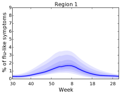
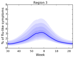
Refer to caption
Refer to caption
Refer to caption
Figure S.2: Samples from the fitted marginal distributions of the weekly flu incidence rates at several regions of the U.S.; samples at larger quantile levels shaded lighter, median in darker blue.
Refer to caption
Figure S.3: Conditional independencies recovered by the MQGM on the wind farms data; each block corresponds to a wind farm, and black indicates dependence.

S.11 Sustainable energy application

We evaluate the ability of MQGM to recover the conditional independencies between several wind farms on the basis of large-scale, hourly wind power measurements; wind power is intermittent, and thus understanding the relationships between wind farms can help farm operators plan. We obtained hourly wind power measurements from July 1, 2009 through September 14, 2010 at seven wind farms (n=877𝑛877n=877, see Hong et al. (2014); Wytock and Kolter (2013); Ali et al. (2016) for details). The primary variables here encode the hourly wind power at a farm over two days (i.e., 48 hours), thus d=7×48=336𝑑748336d=7\times 48=336. Exogenous variables were used to encode forecasted wind power and direction as well as other historical measurements, for a total of q=3417𝑞3417q=3417. We set m=5𝑚5m=5 and r=20𝑟20r=20. Fitting the MQGM here hence requires solving 48×7=33648733648\times 7=336 multiple quantile regression subproblems each of dimension ((3361)×5+3417)×20=101,84033615341720101840\left((336-1)\times 5+3417\right)\times 20=101,840. Each subproblem took roughly 87 minutes, comparable to the algorithm of Wytock and Kolter (2013).

Figure S.3 presents the recovered conditional independencies; the nonzero super- and sub-diagonal entries suggest that at any wind farm, the previous hour’s wind power (naturally) influences the next hour’s, while the nonzero off-diagonal entries, e.g., in the (4,6) block, uncover farms that may influence one another. Wytock and Kolter (2013), whose method placed fifth in a Kaggle competition, as well as Ali et al. (2016) report similar findings (see the left panels of Figures 7 and 3 in these papers, respectively).