Maximizing device-independent randomness from a Bell experiment by optimizing the measurement settings
Abstract
The rates at which a user can generate device-independent quantum random numbers from a Bell-type experiment depend on the measurements that he performs. By numerically optimising over these measurements, we present lower bounds on the randomness generation rates for a family of two-qubit states composed from a mixture of partially entangled states and the completely mixed state. We also report on the randomness generation rates from a tomographic measurement. Interestingly in this case, the randomness generation rates are not monotonic functions of entanglement.
I Introduction
Quantum mechanics is a probabilistic theory. It does not assign definite outcomes to certain measurements. A physicist performing identical measurements on two identically prepared systems might get different measurement outcomes. Quantum mechanics postulates that the outcomes of some measurements are undetermined before the measurement. This randomness in the measurement outcomes has been used to generate random numbers.
It might be argued that the randomness in the measurement outcome is not really undetermined before the measurement. It is perhaps determined by some hidden variables that provide a more complete description of the system, but they are unknown to the physicist. However, this hidden-variable description of nature was recently tested in three Bell test experiments and was found to be incompatible with the observed experimental data Hensen2015 ; Shalm2015 ; Giustina2015 . The observed data were consistent with quantum mechanics. In other words, we see in our experiments that nature behaves randomly, as postulated by quantum mechanics. This implies that if the experimental observations obey some relations and on the condition that the experiment was performed correctly, we can certify the measurement outcomes were undetermined before the measurement was performed. That is, their outcomes generated new random numbers.
The conditions that need to be satisfied are those for a loophole-free Bell experiment. Remarkably, these conditions do not include that the physicist know the mechanisms of the measuring device. This observation makes the realization of a device-independent (DI) quantum random-number generator (QRNG) possible. In a DIQRNG, the user is able to certify the creation of new random numbers despite being ignorant of the device mechanisms.
In certifying the generation of new random numbers, the user trusts that quantum mechanics provides a complete description of nature. Based on the statistics of the measurement outcomes, he can put a bound on the correlations between his measurement outcomes and any other system that exists outside of his lab111We assume that the laboratory is secure.. This bound allows him to extract new random numbers from the measurement outcomes, that is, random numbers which are not correlated to any system outside of his lab.
The first proof-of-concept DIQRNG used entangled photons generated in an atomic ion trap to certify 42 new random numbers over a period of about one month Pironio2010 . More recently, using a more efficient entanglement source, bits of new randomness were created at a rate of bits/s Christensen2013 . Both setups used the Clauser-Horne-Shimony-Holt (CHSH) value Clauser1969 to certify the randomness. The CHSH value is a function of the measurement statistics, and this value sets a lower bound on the DI randomness that can be certified. It turns out that using different Bell operators, that is, different functions of the measurement statistics, will give different equally valid lower bounds to the DI randomness from the same measurement statistics. In Mironowicz2013 , several previously known as well as randomly generated Bell operators were tested and shown to certify varying amount of randomness from the two-qubit Werner state. These operators were chosen in an ad hoc manner, and no single operator was found to be optimal for all the Werner states.
In Nieto-Silleras2014 ; Bancal2014 , the complete measurement statistics were used to obtain a bound on the DI randomness instead of resorting to a specific Bell operator. This gives the highest lower bound on the DI randomness. A by-product of this process is the optimal Bell operator that would have given the same bound. This Bell operator gives the maximum DI randomness for the given measurement statistics.
In a Bell setup for generating new random numbers, the physicist has a choice of the measurement operators to use. By optimizing these operators, he can get a better bound on the DI randomness. This is the question that we address: How much randomness can the physicist certify by using the optimal measurement operator? Recently, this question was also addressed in Mattar2015 for an experimentally relevant optical Bell experiment setup and in Passaro2015 , where the requirement for full device independence was relaxed.
II Background
We consider the usual Bell setup for generating DI random numbers. The user inputs two random and independent measurement settings, and , and receives two measurement outcomes, . In a DI setup, the user does not have any knowledge of the measurement device. The behavior of the apparatus is solely characterized by the conditional probabilities , which we view as the components of the vector . The user will use one measurement setting, , to generate his random numbers; the other settings are only used to obtain bounds on the DI randomness.
Following Nieto-Silleras2014 ; Bancal2014 , the maximum guessing probability for an adversary, Eve, who is constrained by quantum mechanics and has perfect knowledge of the measurement apparatus is
| (1) | |||
| (2) | |||
| (3) |
The notation means that the conditional probabilities can be realized in quantum mechanics. In other words, there exist a state and some measurement operators and such that . The constraint (2) ensures that the weighted sum of the particular behaviors gives the observed behavior . Eve can realize the guessing probability if the measurement device behaves according to with probability and Eve knows the particular behavior of each measurement. For each instant of a particular behavior , Eve’s guess of the measurement outcome will be . If the maximum guessing probability is less than 1, then the lower bound to the amount of certifiable DI randomness is quantified by the minimum entropy .
The optimization problem (1) is a conic linear program, and its dual can be formulated as
| (4) | |||
| (5) |
The solution of the dual program coincides with the solution of the primal program: . The optimization variable corresponds to a Bell expression that gives rise to a guessing probability of . The optimal that achieves the minimum then corresponds to the optimal Bell expression that minimizes Eve’s guessing probability given the behavior .
In general, the optimization problems (1) and (4) can be computationally hard to solve. However the constraints (2) and (5) can be relaxed Navascues2007 ; Navascues2008 to give upper bounds to the guessing probabilities in a way that the programs can be cast as a semidefinite program (SDP) which can be solved efficiently. These relaxations can be progressively tightened to give bounds that are successively tighter.
III Randomness maximization
While the user of a DIRNG has no access to the workings of the device, the physicist who builds the device has a choice of the quantum state and the measurement operators that he wants to implement in the operation of the device. The vector has components which are rank-one projectors and satisfy
| (6) | ||||
For example, if his machine can prepare the pure entangled two-qubit state , then as shown in Dhara2013 , by designing the measurement operators to be projectors along with the angles
| (7) | ||||||||
the device will be able to certify two bits of randomness with the measurement settings . However, if the measurement operators used were not optimal, the machine will exhibit a different behavior and may certify less randomness.
So if the builder can prepare a maximally entangled two-qubit state and use the optimal measurement operator, then the device will be able to certify two bits of randomness, and all is good. However, if the builder is technologically limited to preparing some other state , then in general the measurement operators in (7) will not be optimal anymore. In this case, the builder is then interested in finding the measurement operator he should implement that would certify the maximum randomness222If some outcome symbols given are more unpredictable than others, then more randomness can potentially be extracted by post-selecting a subset of the symbols . Although the post-selection reduce the number of data-points available for randomness extraction, the post-selected data might be more random, which makes it harder to for Eve to guess correctly. The net result can be an increase in the final randomness generation rate Thinh2016 . given that he is restricted to the state . This is the task that we shall now investigate. More precisely, we want to find
| (8) |
where and the vector is constrained by (6). Admittedly, we have not solved this problem. Instead, we present and implement an iterative algorithm in Algorithm 1 that converges to a local maximum of .
The tolerance sets the stopping condition for the algorithm. In step 7, we compute the minimum of guessing probability which corresponds to finding the measurement settings that maximizes the Bell value for a given Bell expression . The guessing probability is a quadratic function of and with the quadratic constraints (6). We can use the Lagrange multiplier method to find the minimum.
While the algorithm might not find the global maximum , it usually finds measurement settings that yield more DI randomness than a randomly chosen measurement setting. In our implementation, we use several initial settings in an attempt to find the global maximum. All SDP calculations were performed using the CVX package for MATLAB Grant2008 ; Grant2014 .
IV Results
We apply our algorithm to the family of states
| (9) |
where and visibility gives the fraction of the state . In the noiseless limit of , arbitrarily close to two bits of DI randomness can be attained in the maximally entangled case when with measurement settings Acin2012 . Two bits of DI randomness are also achievable when is arbitrarily close to zero with measurement settings Acin2012 .
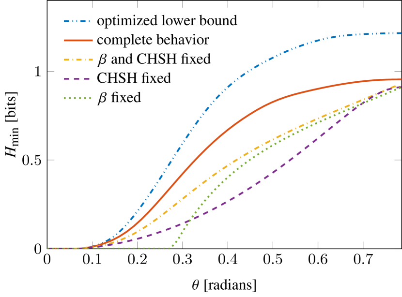
We first consider the case where and the visibility is fixed at . In Fig. 1, we compare the DI randomness from the optimized measurement setting to a bound obtained using a fixed measurement setting as reported in Nieto-Silleras2014 . We see a significant improvement in the certifiable randomness using the optimized measurement settings. For completeness, we also include the certifiable randomness constrained using two specific Bell operators
| (10) | ||||
| (11) |
and also constrained by both operators together Nieto-Silleras2014 using a fixed measurement setting where , , and . The DI randomness bounds using specific operators are always lower than using the complete measurement statistics.
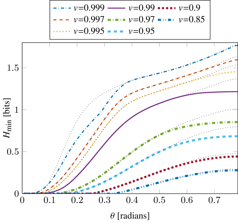
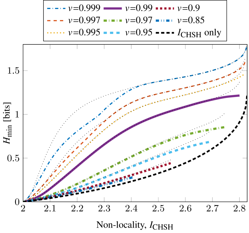
Next, we plot the DI randomness bound as a function of for various visibilities in Fig. 2 for . We also plotted the DI randomness when in the same figure. In most cases, the improvement obtained from using four measurement settings is not very significant. In Fig. 3, we plot the DI randomness as a function of nonlocality as measured by the CHSH value . Relying on the CHSH value alone gives a much lower DI randomness, especially when the state has a high visibility. Even with a maximally entangled two-qubit state, a CHSH value of can only certify bits of randomness.
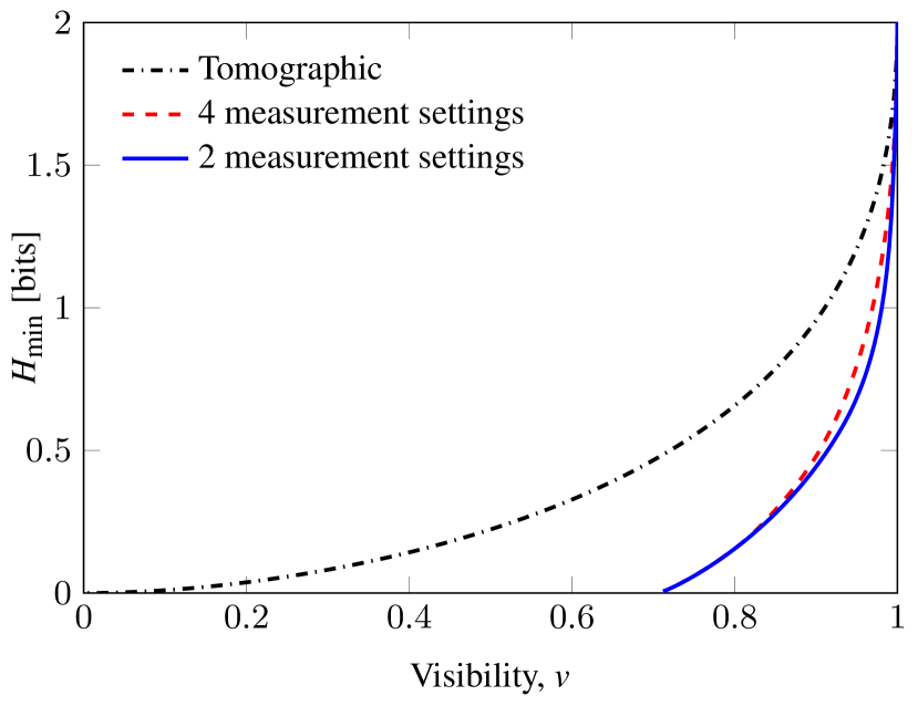
In Fig. 4, we fix the input state to have and plot the DI randomness as a function of visibility for and . There is only a slight increase in the DI randomness bound when going to four measurement settings. The DI randomness increases monotonically with as one would expect. This is because from a high-visibility state, one can always introduce noise to get to a state with lower visibility and attain at least the same DI randomness.
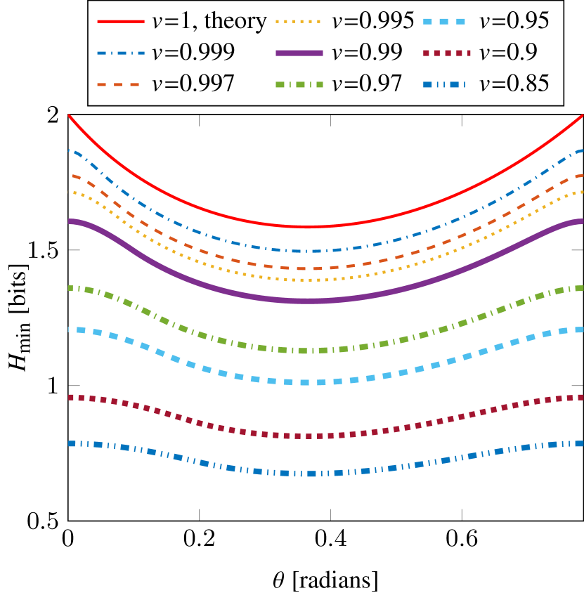
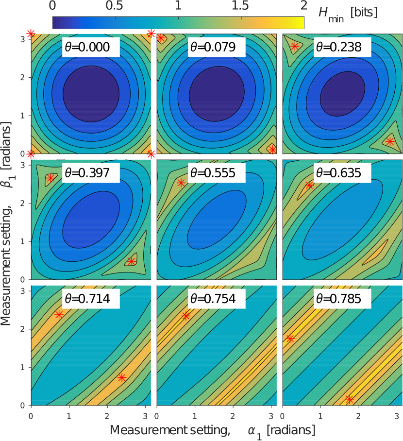
Finally, in the limit when the number of settings becomes large, the DI randomness will be upper bounded by the setup where the user can perform a complete tomography Law2014 . In this case, the constraint (2) is replaced by a constraint on the quantum states with . The constraints that is positive mean that programs (1) and (4) are already SDPs. We plot the tomographic randomness rate in Fig. 5. For a fixed , the tomographic randomness rates decrease with . However, the tomographic randomness rates are not monotonic in for a fixed . For the same , starting with a state with small entanglement (low ) can still yield the same amount of randomness as a state with large entanglement ( near ). The dip in the randomness rates when is unlikely due to the algorithm being stuck in a local maximum. We check this numerically by scanning the whole parameter space. For the case of a qubit pair input that we are considering, the measurement directions that the user uses to generate his tomographic randomness can be parametrized by the Bloch vector angles and . Some typical tomographic randomness rates are shown in Fig. 6 as a function of the two Bloch vectors.
In Fig. 4, we plot the randomness from a tomographic measurement when as a function of . We find no improvement compared to the results reported in Law2014 . The measurement used there,
| (12) |
indeed attains the maximum randomness we found.
When the visibility is exactly unity, the quantum state that the user has is a pure state. For this, Eve’s guessing probability can be calculated exactly and then maximized over the user’s measurements. The final result is
| (13) |
where characterizes the measurement direction and is given by solving
| (14) |
The min-entropy from this guessing probability is plotted as the top line in Fig. 5. We see that two bits of randomness are achievable only when the state is maximally entangled or when it is separable.
V Conclusions
The amount of randomness generated from a DIQRNG can be improved by optimizing the measurement setting. However, for the two-qubit state considered, the additional improvement achieved by using four measurement settings on each side is in most cases not significant. There is a disadvantage in having more measurement settings: the experimental setup is more complicated and more data are needed to characterize the measurements. This is not justified by the minimal increase in the randomness generation rates.
Acknowledgements.
We acknowledge the support of the Australian Research Council Centre of Excellence for Quantum Computation and Communication Technology (Project No. CE110001027).References
- (1) B. Hensen, H. Bernien, A. E. Dréau, A. Reiserer, N. Kalb, M. S. Blok, J. Ruitenberg, R. F. L. Vermeulen, R. N. Schouten, C. Abellán, W. Amaya, V. Pruneri, M. W. Mitchell, M. Markham, D. J. Twitchen, D. Elkouss, S. Wehner, T. H. Taminiau, and R. Hanson. Loophole-free Bell inequality violation using electron spins separated by 1.3 kilometres. Nature, 526(7575):682–686, October 2015.
- (2) Lynden K. Shalm, Evan Meyer-Scott, Bradley G. Christensen, Peter Bierhorst, Michael A. Wayne, Martin J. Stevens, Thomas Gerrits, Scott Glancy, Deny R. Hamel, Michael S. Allman, Kevin J. Coakley, Shellee D. Dyer, Carson Hodge, Adriana E. Lita, Varun B. Verma, Camilla Lambrocco, Edward Tortorici, Alan L. Migdall, Yanbao Zhang, Daniel R. Kumor, William H. Farr, Francesco Marsili, Matthew D. Shaw, Jeffrey A. Stern, Carlos Abellán, Waldimar Amaya, Valerio Pruneri, Thomas Jennewein, Morgan W. Mitchell, Paul G. Kwiat, Joshua C. Bienfang, Richard P. Mirin, Emanuel Knill, and Sae Woo Nam. Strong loophole-free test of local realism. Phys. Rev. Lett., 115:250402, Dec 2015.
- (3) Marissa Giustina, Marijn A. M. Versteegh, Sören Wengerowsky, Johannes Handsteiner, Armin Hochrainer, Kevin Phelan, Fabian Steinlechner, Johannes Kofler, Jan-Åke Larsson, Carlos Abellán, Waldimar Amaya, Valerio Pruneri, Morgan W. Mitchell, Jörn Beyer, Thomas Gerrits, Adriana E. Lita, Lynden K. Shalm, Sae Woo Nam, Thomas Scheidl, Rupert Ursin, Bernhard Wittmann, and Anton Zeilinger. Significant-loophole-free test of Bell’s theorem with entangled photons. Phys. Rev. Lett., 115:250401, Dec 2015.
- (4) S. Pironio, A. Acin, S. Massar, A. Boyer de la Giroday, D. N. Matsukevich, P. Maunz, S. Olmschenk, D. Hayes, L. Luo, T. A. Manning, and et al. Random numbers certified by Bell’s theorem. Nature, 464(7291):1021–1024, Apr 2010.
- (5) B. G. Christensen, K. T. McCusker, J. B. Altepeter, B. Calkins, T. Gerrits, A. E. Lita, A. Miller, L. K. Shalm, Y. Zhang, S. W. Nam, and et al. Detection-loophole-free test of quantum nonlocality, and applications. Phys. Rev. Lett., 111(13), Sep 2013.
- (6) John F. Clauser, Michael A. Horne, Abner Shimony, and Richard A. Holt. Proposed experiment to test local hidden-variable theories. Phys. Rev. Lett., 23(15):880–884, Oct 1969.
- (7) Piotr Mironowicz and Marcin Pawlowski. Robustness of quantum-randomness expansion protocols in the presence of noise. Phys. Rev. A, 88(3), Sep 2013.
- (8) O Nieto-Silleras, S Pironio, and J Silman. Using complete measurement statistics for optimal device-independent randomness evaluation. New J. Phys., 16(1):013035, Jan 2014.
- (9) Jean-Daniel Bancal, Lana Sheridan, and Valerio Scarani. More randomness from the same data. New J. Phys., 16(3):033011, Mar 2014.
- (10) Alejandro Mattar, Paul Skrzypczyk, Jonatan Bohr Brask, Daniel Cavalcanti, and Antonio Acin. Optimal randomness generation from optical Bell experiments. New J. Phys., 17(2):022003, Feb 2015.
- (11) Elsa Passaro, Daniel Cavalcanti, Paul Skrzypczyk, and Antonio Acín. Optimal randomness certification in the quantum steering and prepare-and-measure scenarios. New J. Phys., 17(11):113010, Oct 2015.
- (12) Miguel Navascués, Stefano Pironio, and Antonio Acín. Bounding the set of quantum correlations. Phys. Rev. Lett., 98:010401, Jan 2007.
- (13) Miguel Navascués, Stefano Pironio, and Antonio Acín. A convergent hierarchy of semidefinite programs characterizing the set of quantum correlations. New J. of Phys., 10(7):073013, Jul 2008.
- (14) Chirag Dhara, Giuseppe Prettico, and Antonio Acín. Maximal quantum randomness in Bell tests. Phys. Rev. A, 88:052116, Nov 2013.
- (15) Michael Grant and Stephen Boyd. Graph implementations for nonsmooth convex programs. In V. Blondel, S. Boyd, and H. Kimura, editors, Recent Advances in Learning and Control, Lecture Notes in Control and Information Sciences, pages 95–110. Springer-Verlag Limited, 2008. http://stanford.edu/~boyd/graph_dcp.html.
- (16) Michael Grant and Stephen Boyd. CVX: Matlab software for disciplined convex programming, version 2.1. http://cvxr.com/cvx, March 2014.
- (17) Antonio Acín, Serge Massar, and Stefano Pironio. Randomness versus nonlocality and entanglement. Phys. Rev. Lett., 108:100402, Mar 2012.
- (18) Yun Zhi Law, Le Phuc Thinh, Jean-Daniel Bancal, and Valerio Scarani. Quantum randomness extraction for various levels of characterization of the devices. J. Phys. A: Math. Theor., 47(42):424028, Oct 2014.
- (19) Le Phuc Thinh, Gonzalo de la Torre, Jean-Daniel Bancal, Stefano Pironio, and Valerio Scarani. Randomness in post-selected events. New J. Phys., 18(3):035007, Mar 2016.