\numberofauthors

2

A Greedy Approach to Adapting the Trace Parameter for Temporal Difference Learning

\alignauthorMartha White
\affaddrDepartment of Computer Science
\affaddrIndiana University
\affaddrBloomington, IN 47405, USA
\alignauthorAdam White
\affaddrDepartment of Computer Science
\affaddrIndiana University
\affaddrBloomington, IN 47405, USA
martha@indiana.edu adamw@indiana.edu
Abstract

One of the main obstacles to broad application of reinforcement learning methods is the parameter sensitivity of our core learning algorithms. In many large-scale applications, online computation and function approximation represent key strategies in scaling up reinforcement learning algorithms. In this setting, we have effective and reasonably well understood algorithms for adapting the learning-rate parameter, online during learning. Such meta-learning approaches can improve robustness of learning and enable specialization to current task, improving learning speed. For temporal-difference learning algorithms which we study here, there is yet another parameter, ฮป๐œ†\lambda, that similarly impacts learning speed and stability in practice. Unfortunately, unlike the learning-rate parameter, ฮป๐œ†\lambda parametrizes the objective function that temporal-difference methods optimize. Different choices of ฮป๐œ†\lambda produce different fixed-point solutions, and thus adapting ฮป๐œ†\lambda online and characterizing the optimization is substantially more complex than adapting the learning-rate parameter. There are no meta-learning method for ฮป๐œ†\lambda that can achieve (1) incremental updating, (2) compatibility with function approximation, and (3) maintain stability of learning under both on and off-policy sampling. In this paper we contribute a novel objective function for optimizing ฮป๐œ†\lambda as a function of state rather than time. We derive a new incremental, linear complexity ฮป๐œ†\lambda-adaption algorithm that does not require offline batch updating or access to a model of the world, and present a suite of experiments illustrating the practicality of our new algorithm in three different settings. Taken together, our contributions represent a concrete step towards black-box application of temporal-difference learning methods in real world problems.

Key Words.:
Reinforcement learning; temporal difference learning; off-policy learning

1 Introduction

In reinforcement learning, the training data is produced by an adaptive learning agentโ€™s interaction with its environment, which makes tuning the parameters of the learning process both challenging and essential for good performance. In the online setting we study here, the agent-environment interaction produces an unending stream of temporally correlated data. In this setting there is no testing-training split, and thus the agentโ€™s learning process must be robust and adapt to new situations not considered by the human designer. Robustness is often critically related to the values of a small set parameters that control the learning process (e.g., the step-size parameter). In real-world applications, however, we cannot expect to test a large range of theses parameter values, in all the situations the agent may face, to ensure good performanceโ€”common practice in empirical studies. Unfortunately, safe values of these parameters are usually problem dependent. For example, in off-policy learning (e.g., learning from demonstrations), large importance sampling ratios can destabilize provably convergent gradient temporal difference learning methods, when the parameters are not set in a very particular way (ฮป=0๐œ†0\lambda=0) white2015thesis . In such situations, we turn to meta-learning algorithms that can adapt the parameters of the agent continuously, based on the stream of experience and some notion of the agentโ€™s own learning progress. These meta-learning approaches can potentially improve robustness, and also help the agent specialize to the current task, and thus improve learning speed.

Temporal difference learning methods make use of two important parameters: the step-size parameter and the trace-decay parameter. The step-size parameter is the same as those used in stochastic gradient descent, and there are algorithms available for adjusting this parameter online, in reinforcement learning dabney2012adaptive . For the trace decay parameter, on the other hand, we have no generally applicable meta-learning algorithms that are compatible with function approximation, incremental processing, and off-policy sampling.

The difficulty in adapting the trace decay parameter, ฮป๐œ†\lambda, mainly arises from the fact that it has seemingly multiple roles and also influences the fixed-point solution. This parameter was introduced in Samuelโ€™s checker player samuel1959some , and later described as interpolation parameter between offline TD(0) and Monte-Carlo sampling (TD(ฮป=1๐œ†1\lambda=1) by Suttonsutton1988learning . It has been empirically demonstrated that values of ฮป๐œ†\lambda between zero and one often perform the best in practice sutton1988learning ; sutton1998introduction ; vanseijen2014true . This trace parameter can also be viewed as a bias-variance trade-off parameter: ฮป๐œ†\lambda closer to one is less biased but likely to have higher variance, where ฮป๐œ†\lambda closer to zero is more biased, but likely has lower variance. However, it has also been described as a credit-assignment parameter singh1996reinforcement , as a method to encode probability of transitions sutton1994onstep , a way to incorporate the agentโ€™s confidence in its value function estimates sutton1998introduction ; tesauro1992practical , and as an averaging of n-step returns sutton1998introduction . Selecting ฮป๐œ†\lambda is further complicated by the fact that ฮป๐œ†\lambda is a part of the problem definition: the solution to the Bellman fixed point equation is dependent on the choice of ฮป๐œ†\lambda (unlike the step-size parameter).

There are few approaches for setting ฮป๐œ†\lambda, and most existing work is limited to special cases. For instance, several approaches have analyzed setting ฮป๐œ†\lambda for variants of TD that were introduced to simplify the analysis, including phased TD kearns2000bias and TD(ฮป)โˆ—{}^{*}(\lambda) schapire1996ontheworst . Though both provide valuable insights into the role of ฮป๐œ†\lambda, the analysis does not easily extend to conventional TD algorithms. Sutton and Singh sutton1994onstep investigated tuning both the learning rate parameter and ฮป๐œ†\lambda, and proposed two meta-learning algorithms. The first assumes the problem can be modeled by an acyclic MDP, and the other requires access to the transition model of the MDP. Singh and Dayan singh1996analytical and Kearns and Singh kearns2000bias contributed extensive simulation studies of the interaction between ฮป๐œ†\lambda and other agent parameters on a chain MDP, but again relied on access to the model and offline computation. The most recent study downey2010temporal explores a Bayesian variant of TD learning, but requires a batch of samples and can only be used off-line. Finally, Konidaris et al.ย konidaris2011td introduce TDฮณ as a method to remove the ฮป๐œ†\lambda parameter altogether. Their approach, however, has not been extended to the off-policy setting and their full algorithm is too computationally expensive for incremental estimation, while their incremental variant introduces a sensitive meta-parameter. Although this long-history of prior work has helped develop our intuitions about ฮป๐œ†\lambda, the available solutions are still far from the use cases outlined above.

This paper introduces an new objective based on locally optimizing bias-variance, which we use to develop an efficient, incremental algorithm for learning state-based ฮป๐œ†\lambda. We use a forward-backward analysis sutton1998introduction to derive an incremental algorithm to estimate the variance of the return. Using this estimate, we obtain a closed-form estimate of ฮป๐œ†\lambda on each time-step. Finally, we empirically demonstrate the generality of the approach with a suite of on-policy and off-policy experiments. Our results show that our new algorithm, ฮป๐œ†\lambda-greedy, is consistently amongst the best performing, adapting as the problem changes, whereas any fixed approach works well in some settings and poorly in anothers.

2 Background

We model the agentโ€™s interaction with an unknown environment as a discrete time Markov Decision Process (MDP). A MDP is characterized by a finite set of states ๐’ฎ๐’ฎ\mathcal{S}, set of actions ๐’œ๐’œ\mathcal{A}, a reward function r:๐’ฎร—๐’ฎโ†’โ„:๐‘Ÿโ†’๐’ฎ๐’ฎโ„r:\mathcal{S}\times\mathcal{S}\rightarrow\mathbb{R}, and generalized state-based discount ฮณ:๐’ฎโˆˆ[0,1]:๐›พ๐’ฎ01\gamma:\mathcal{S}\in[0,1], which encodes the level of discounting per-state (e.g., a common setting is a constant discount for all states). On each of a discrete number of timesteps, t=1,2,3,โ€ฆ๐‘ก123โ€ฆt=1,2,3,\ldots, the agent observes the current state Stsubscript๐‘†๐‘กS_{t}, selects an action Atsubscript๐ด๐‘กA_{t}, according to its target policy ฯ€:๐’ฎร—๐’œโ†’[0,1]:๐œ‹โ†’๐’ฎ๐’œ01\pi:\mathcal{S}\times\mathcal{A}\rightarrow[0,1], and the environment transitions to a new state St+1subscript๐‘†๐‘ก1S_{t+1} and emits a reward Rt+1subscript๐‘…๐‘ก1R_{t+1}. The state transitions are governed by the transition function P:๐’ฎร—๐’œร—๐’ฎโ†’[0,1]:๐‘ƒโ†’๐’ฎ๐’œ๐’ฎ01P:\mathcal{S}\times\mathcal{A}\times\mathcal{S}\rightarrow[0,1], where Pโ€‹(St,At,St+1)๐‘ƒsubscript๐‘†๐‘กsubscript๐ด๐‘กsubscript๐‘†๐‘ก1P(S_{t},A_{t},S_{t+1}) denotes the probability of transitioning from Stsubscript๐‘†๐‘กS_{t} to St+1subscript๐‘†๐‘ก1S_{t+1}, due to action Atsubscript๐ด๐‘กA_{t}. At timestep t๐‘กt, the future rewards are summarized by the Monte Carlo (MC) return Gtโˆˆโ„subscript๐บ๐‘กโ„G_{t}\in\mathbb{R} defined by the infinite discounted sum

Gtsubscript๐บ๐‘ก\displaystyle G_{t}\ =defโ€‹Rt+1+ฮณt+1โ€‹Rt+2+ฮณt+1โ€‹ฮณt+2โ€‹Rt+3+โ€ฆdefsubscript๐‘…๐‘ก1subscript๐›พ๐‘ก1subscript๐‘…๐‘ก2subscript๐›พ๐‘ก1subscript๐›พ๐‘ก2subscript๐‘…๐‘ก3โ€ฆ\displaystyle\overset{\text{def}}{=}R_{t+1}+\gamma_{t+1}R_{t+2}+\gamma_{t+1}\gamma_{t+2}R_{t+3}+\ldots โ–ทฮณt=ฮณโ€‹(St)โ–ทsubscript๐›พ๐‘ก๐›พsubscript๐‘†๐‘ก\displaystyle\triangleright\gamma_{t}=\gamma(S_{t})
=Rt+1+ฮณt+1โ€‹Gt+1.absentsubscript๐‘…๐‘ก1subscript๐›พ๐‘ก1subscript๐บ๐‘ก1\displaystyle=R_{t+1}+\gamma_{t+1}G_{t+1}.

The agentโ€™s objective is to estimate the expected return or value function, vฯ€:๐’ฎโ†’โ„:superscript๐‘ฃ๐œ‹โ†’๐’ฎโ„v^{\pi}:\mathcal{S}\rightarrow\mathbb{R}, defined as vฯ€โ€‹(s)โ€‹=defโ€‹๐”ผโ€‹[Gt|St=s,Atโˆผฯ€]superscript๐‘ฃ๐œ‹๐‘ def๐”ผdelimited-[]formulae-sequenceconditionalsubscript๐บ๐‘กsubscript๐‘†๐‘ก๐‘ similar-tosubscript๐ด๐‘ก๐œ‹v^{\pi}(s)\overset{\text{def}}{=}\mathbb{E}[G_{t}|S_{t}=s,A_{t}\sim\pi]. We estimate the value function using the standard framework of linear function approximation. We assume the state of the environment at time t๐‘กt can be characterized by a fixed-length feature vector ๐ฑtโˆˆโ„nsubscript๐ฑ๐‘กsuperscriptโ„๐‘›\mathbf{x}_{t}\in\mathbb{R}^{n}, where nโ‰ช|๐’ฎ|much-less-than๐‘›๐’ฎn\ll|\mathcal{S}|; implicitly, ๐ฑtsubscript๐ฑ๐‘ก\mathbf{x}_{t} is a function of the random variable Stsubscript๐‘†๐‘กS_{t}. The agent uses a linear estimate of the value of Stsubscript๐‘†๐‘กS_{t}: the inner product of ๐ฑtsubscript๐ฑ๐‘ก\mathbf{x}_{t} and a modifiable set of weights ๐ฐโˆˆโ„n๐ฐsuperscriptโ„๐‘›\mathbf{w}\in\mathbb{R}^{n}, v^โ€‹(St,๐ฐ)โ€‹=defโ€‹๐ฑtโŠคโ€‹๐ฐ^๐‘ฃsubscript๐‘†๐‘ก๐ฐdefsuperscriptsubscript๐ฑ๐‘กtop๐ฐ\hat{v}(S_{t},\mathbf{w})\overset{\text{def}}{=}\mathbf{x}_{t}^{\top}\mathbf{w}, with mean-squared error (MSE) =โˆ‘sโˆˆ๐’ฎdโ€‹(s)โ€‹(vโ€‹(s)โˆ’v^โ€‹(s,๐ฐ))2absentsubscript๐‘ ๐’ฎ๐‘‘๐‘ superscript๐‘ฃ๐‘ ^๐‘ฃ๐‘ ๐ฐ2=\sum_{s\in\mathcal{S}}d(s)(v(s)-\hat{v}(s,\mathbf{w}))^{2}, where d:๐’ฎโ†’[0,1]:๐‘‘โ†’๐’ฎ01d:\mathcal{S}\rightarrow[0,1] encodes the distribution over states induced by the agentโ€™s behavior in the MDP.

Instead of estimating the expected value of Gtsubscript๐บ๐‘กG_{t}, we can estimate a ฮป๐œ†\lambda-return that is expected to have lower variance

Gtฮปโ€‹=defโ€‹Rt+1+ฮณt+1โ€‹[(1โˆ’ฮปt+1)โ€‹๐ฑt+1โŠคโ€‹๐ฐ+ฮปt+1โ€‹Gt+1ฮป],subscriptsuperscript๐บ๐œ†๐‘กdefsubscript๐‘…๐‘ก1subscript๐›พ๐‘ก1delimited-[]1subscript๐œ†๐‘ก1superscriptsubscript๐ฑ๐‘ก1top๐ฐsubscript๐œ†๐‘ก1subscriptsuperscript๐บ๐œ†๐‘ก1\displaystyle G^{\lambda}_{t}\overset{\text{def}}{=}R_{t+1}+\gamma_{t+1}[(1-\lambda_{t+1})\mathbf{x}_{t+1}^{\top}\mathbf{w}+\lambda_{t+1}G^{\lambda}_{t+1}],

where the trace decay function ฮป:๐’ฎโ†’[0,1]:๐œ†โ†’๐’ฎ01\lambda:\mathcal{S}\rightarrow[0,1] specifies the trace parameter as a function of state. The trace parameter ฮปt+1=ฮปโ€‹(st+1)subscript๐œ†๐‘ก1๐œ†subscript๐‘ ๐‘ก1\lambda_{t+1}=\lambda(s_{t+1}) averages the estimate of the return, ๐ฑt+1โŠคโ€‹๐ฐsuperscriptsubscript๐ฑ๐‘ก1top๐ฐ\mathbf{x}_{t+1}^{\top}\mathbf{w}, and the ฮป๐œ†\lambda-return starting on the next step, Gt+1ฮปsubscriptsuperscript๐บ๐œ†๐‘ก1G^{\lambda}_{t+1}. When ฮป=1๐œ†1\lambda=1, Gtฮปsubscriptsuperscript๐บ๐œ†๐‘กG^{\lambda}_{t} becomes the MC return Gtsubscript๐บ๐‘กG_{t}, and the value function can be estimated by averaging rollouts from each state. When ฮป=0๐œ†0\lambda=0, Gtฮปsubscriptsuperscript๐บ๐œ†๐‘กG^{\lambda}_{t} becomes equal to the one-step ฮป๐œ†\lambda-return, Rt+1+ฮณt+1โ€‹๐ฑt+1โŠคโ€‹๐ฐ,subscript๐‘…๐‘ก1subscript๐›พ๐‘ก1superscriptsubscript๐ฑ๐‘ก1top๐ฐR_{t+1}+\gamma_{t+1}\mathbf{x}_{t+1}^{\top}\mathbf{w}, and the value function can be estimated by the linear TD(0) algorithm. The ฮป๐œ†\lambda-return when ฮปโˆˆ(0,1)๐œ†01\lambda\in(0,1) is often easier to estimate than MC, and yields more accurate predictions than using the one-step return. The intuition, is that the for large ฮป๐œ†\lambda, the estimate is high-variance due to averaging possibly long trajectories of noisy rewards, but less bias because the initial biased estimates of the value function participate less in the computation of the return. In the case of low ฮป๐œ†\lambda, the estimate has lower-variance because fewer potentially noisy rewards participate in Gtฮปsubscriptsuperscript๐บ๐œ†๐‘กG^{\lambda}_{t}, but there is more bias due to the increase role of the initial value function estimates. We further discuss the intuition for this parameter in the next section.

The generalization to state-based ฮณ๐›พ\gamma and ฮป๐œ†\lambda have not yet been widely considered, though the concept was introduced more than a decade ago sutton1995td ; sutton1999between and the generalization shown to be useful sutton1995td ; maei2010gq ; modayil2014multi ; sutton2015anemphatic . The Bellman operator can be generalized to include state-based ฮณ๐›พ\gamma and ฮป๐œ†\lambda (see (sutton2015anemphatic, , Equation 29)), where the choice of ฮป๐œ†\lambda per-state influences the fixed point. Time-based ฮป๐œ†\lambda, on the other hand, would not result in a well-defined fixed point. Therefore, to ensure a well-defined fixed point, we will design an objective and algorithm to learn a state-based ฮป๐œ†\lambda.

This paper considers both on- and off-policy policy evaluation. In the more conventional on-policy learning setting, we estimate vฯ€โ€‹(s)superscript๐‘ฃ๐œ‹๐‘ v^{\pi}(s) based on samples generated while selecting actions according to the target policy ฯ€๐œ‹\pi. In the off-policy case, we estimate vฯ€โ€‹(s)superscript๐‘ฃ๐œ‹๐‘ v^{\pi}(s) based on samples generated while selecting actions according to the behavior policy ฮผ:๐’ฎร—๐’œโ†’[0,1]:๐œ‡โ†’๐’ฎ๐’œ01\mu:\mathcal{S}\times\mathcal{A}\rightarrow[0,1], and ฯ€โ‰ ฮผ๐œ‹๐œ‡\pi\neq\mu. In order to learn v^^๐‘ฃ\hat{v} in both these settings we use the GTD(ฮป๐œ†\lambda) algorithm maei2011gradient specified by the following update equations:

ฯtโ€‹=defโ€‹ฯ€โ€‹(St,At)ฮผโ€‹(St,At)โ–ทimportance sampling ratiosubscript๐œŒ๐‘กdef๐œ‹subscript๐‘†๐‘กsubscript๐ด๐‘ก๐œ‡subscript๐‘†๐‘กsubscript๐ด๐‘กโ–ทimportance sampling ratio\displaystyle\rho_{t}\overset{\text{def}}{=}\frac{\pi(S_{t},A_{t})}{\mu(S_{t},A_{t})}\hskip 56.9055pt\triangleright\text{importance sampling ratio}
๐žtโ€‹=defโ€‹ฯtโ€‹(ฮณtโ€‹ฮปtโ€‹๐žtโˆ’1+๐ฑt)โ–ทeligibility tracesubscript๐ž๐‘กdefsubscript๐œŒ๐‘กsubscript๐›พ๐‘กsubscript๐œ†๐‘กsubscript๐ž๐‘ก1subscript๐ฑ๐‘กโ–ทeligibility trace\displaystyle\mathbf{e}_{t}\overset{\text{def}}{=}\rho_{t}(\gamma_{t}\lambda_{t}\mathbf{e}_{t-1}+\mathbf{x}_{t})\hskip 54.06006pt\triangleright\text{eligibility trace}
ฮดtโ€‹=defโ€‹Rt+1+ฮณtโ€‹๐ฑt+1โŠคโ€‹๐ฐtโˆ’๐ฑtโŠคโ€‹๐ฐtโ–ทTD errorsubscript๐›ฟ๐‘กdefsubscript๐‘…๐‘ก1subscript๐›พ๐‘กsuperscriptsubscript๐ฑ๐‘ก1topsubscript๐ฐ๐‘กsuperscriptsubscript๐ฑ๐‘กtopsubscript๐ฐ๐‘กโ–ทTD error\displaystyle\delta_{t}\overset{\text{def}}{=}R_{t+1}+\gamma_{t}\mathbf{x}_{t+1}^{\top}\mathbf{w}_{t}-\mathbf{x}_{t}^{\top}\mathbf{w}_{t}\hskip 22.76228pt\triangleright\text{TD error}
๐ฐt+1โ†๐ฐt+ฮฑโ€‹(ฮดtโ€‹๐žtโˆ’ฮณtโ€‹(1โˆ’ฮปt+1)โ€‹๐žtโŠคโ€‹๐กtโ€‹๐ฑt+1)โ†subscript๐ฐ๐‘ก1subscript๐ฐ๐‘ก๐›ผsubscript๐›ฟ๐‘กsubscript๐ž๐‘กsubscript๐›พ๐‘ก1subscript๐œ†๐‘ก1superscriptsubscript๐ž๐‘กtopsubscript๐ก๐‘กsubscript๐ฑ๐‘ก1\displaystyle\mathbf{w}_{t+1}\leftarrow\mathbf{w}_{t}+\alpha(\delta_{t}\mathbf{e}_{t}-\gamma_{t}(1-\lambda_{t+1})\mathbf{e}_{t}^{\top}\mathbf{h}_{t}\mathbf{x}_{t+1})
๐กt+1โ†๐กt+ฮฑ๐กโ€‹(ฮดtโ€‹๐žtโˆ’๐ฑtโŠคโ€‹๐กt)โ€‹๐ฑtโ–ทauxiliary weightsโ†subscript๐ก๐‘ก1subscript๐ก๐‘กsubscript๐›ผ๐กsubscript๐›ฟ๐‘กsubscript๐ž๐‘กsuperscriptsubscript๐ฑ๐‘กtopsubscript๐ก๐‘กsubscript๐ฑ๐‘กโ–ทauxiliary weights\displaystyle\mathbf{h}_{t+1}\leftarrow\mathbf{h}_{t}+\alpha_{\mathbf{h}}(\delta_{t}\mathbf{e}_{t}-\mathbf{x}_{t}^{\top}\mathbf{h}_{t})\mathbf{x}_{t}\hskip 14.22636pt\triangleright\text{auxiliary weights}

with step-sizes ฮฑ,ฮฑ๐กโˆˆโ„+๐›ผsubscript๐›ผ๐กsuperscriptโ„\alpha,\alpha_{\mathbf{h}}\in\mathbb{R}^{+} and an arbitrary initial ๐ฐ0,๐ก0subscript๐ฐ0subscript๐ก0\mathbf{w}_{0},\mathbf{h}_{0} (e.g., the zero vector). The importance sampling ratio ฯtโˆˆโ„+subscript๐œŒ๐‘กsuperscriptโ„\rho_{t}\in\mathbb{R}^{+} facilitates learning about rewards as if they were generated by following ฯ€๐œ‹\pi, instead of ฮผ๐œ‡\mu. This ratio can be very large if ฮผโ€‹(St,At)๐œ‡subscript๐‘†๐‘กsubscript๐ด๐‘ก\mu(S_{t},A_{t}) is small, which can compound and destabilize learning.

3 Objective for trace adaptation

To obtain an objective for selecting ฮป๐œ†\lambda, we need to clarify its role. Although ฮป๐œ†\lambda was not introduced with the goal of trading off bias and variance sutton1988learning , several algorithms and significant theory have developed its role as such kearns2000bias ; schapire1996ontheworst . Other roles have been suggested; however, as we discuss below, each of them can still be thought of as a bias-variance trade-off.

The ฮป๐œ†\lambda parameter has been described as a credit assignment parameter, which allows TD(ฮป๐œ†\lambda) to perform multi-step updates on each time step. On each update, ฮปtsubscript๐œ†๐‘ก\lambda_{t} controls the amount of credit assigned to previous transitions, using the eligibility trace ๐ž๐ž\mathbf{e}. For ฮปtsubscript๐œ†๐‘ก\lambda_{t} close to 1, TD(ฮป๐œ†\lambda) assigns more credit for the current reward to previous transitions, resulting in updates to many states along the current trajectory. Conversely, for ฮปt=0subscript๐œ†๐‘ก0\lambda_{t}=0, the eligibility trace is cleared and no credit is assigned back in time, performing a single-step TD(0) update. In fact, this intuition can still be thought of as a bias-variance trade-off. In terms of credit assignment, we ideally always want to send maximal credit ฮป=1๐œ†1\lambda=1, but decayed by ฮณ๐›พ\gamma, for the current reward, which is also unbiased. In practice, however, this often leads to high variance, and thus we mitigate the variance by choosing ฮป๐œ†\lambda less than one and speed learning overall, but introduce bias.

Another interpretation is that ฮป๐œ†\lambda should be set to reflect confidence in value function estimates tesauro1992practical ; sutton1998introduction . If your confidence in the value estimate of state s๐‘ s is high, then ฮปโ€‹(s)๐œ†๐‘ \lambda(s) should be close to 0, meaning we trust the estimates provided by v^^๐‘ฃ\hat{v}. If your confidence is low, suspecting that v^^๐‘ฃ\hat{v} may be inaccurate, then ฮปโ€‹(s)๐œ†๐‘ \lambda(s) should be close to 1, meaning we trust observed rewards more. For example in states that are indistinguishable with function approximation (i.e., aliased states), we should not trust the v^^๐‘ฃ\hat{v} as much. This intuition similarly translates to bias-variance. If v^^๐‘ฃ\hat{v} is accurate, then decreasing ฮปโ€‹(s)๐œ†๐‘ \lambda(s) does not incur (much) bias, but can significantly decrease the variance since v^^๐‘ฃ\hat{v} gives the correct value. If v^^๐‘ฃ\hat{v} is inaccurate, then the increased bias is not worth the reduced variance, so ฮปโ€‹(s)๐œ†๐‘ \lambda(s) should be closer to 1 to use actual (potentially high-variance) samples.

Finally, a less commonly discussed interpretation is that ฮป๐œ†\lambda acts as parameter that simulates a form of experience replay (or model-based simulation of trajectories). One can imagine that sending back information in eligibility traces is like simulating experience from a model, where the model could be a set of trajectories, as in experience replay lin1992self . If ฮป=1๐œ†1\lambda=1, the traces are longer and each update gets more trajectory information, or experience replay. If a trajectory from a point, however, was unlikely (e.g., a rare transition), we may not want to use that information. Such an approach was taken by Sutton and Singh sutton1994onstep , where ฮป๐œ†\lambda was set to the transition probabilities. Even in this model-based interpretation, the goal in setting ฮป๐œ†\lambda becomes one of mitigating variance, without incurring too much bias.

Optimizing this bias-variance trade-off, however, is difficult because ฮป๐œ†\lambda affects the return we are approximating. Jointly optimizing for ฮป๐œ†\lambda across all time-steps is generally not feasible. One strategy is to take a batch approach, where the optimal ฮป๐œ†\lambda is determined after seeing all the data downey2010temporal . Our goal, however, is to develop approaches for the online setting, where future states, actions, rewards and the influence of ฮป๐œ†\lambda have yet to be observed.

We propose to take a greedy approach: on each time step select ฮปt+1subscript๐œ†๐‘ก1\lambda_{t+1} to optimize the bias-variance trade-off for only this step. This greedy objective corresponds to minimizing the mean-squared error between the unbiased ฮป=1๐œ†1\lambda=1 return Gtsubscript๐บ๐‘กG_{t} and the estimate G^tsubscript^๐บ๐‘ก\hat{G}_{t} with ฮปt+1โˆˆ[0,1]subscript๐œ†๐‘ก101\lambda_{t+1}\in[0,1] with ฮป=1๐œ†1\lambda=1 into the future after t+1๐‘ก1t+1

G^tโ€‹=defโ€‹ฯtโ€‹(Rt+1+ฮณt+1โ€‹[(1โˆ’ฮปt+1)โ€‹๐ฑt+1โŠคโ€‹๐ฐt+ฮปt+1โ€‹Gt+1โŸMonte Carlo]).subscript^๐บ๐‘กdefsubscript๐œŒ๐‘กsubscript๐‘…๐‘ก1subscript๐›พ๐‘ก1delimited-[]1subscript๐œ†๐‘ก1superscriptsubscript๐ฑ๐‘ก1topsubscript๐ฐ๐‘กsubscript๐œ†๐‘ก1subscriptโŸsubscript๐บ๐‘ก1Monte Carlo\displaystyle\hat{G}_{t}\overset{\text{def}}{=}\rho_{t}(R_{t+1}+\gamma_{t+1}[(1\!-\!\lambda_{t+1})\mathbf{x}_{t+1}^{\top}\mathbf{w}_{t}+\lambda_{t+1}\underbrace{G_{t+1}}_{\makebox[0.0pt]{\text{\tiny Monte Carlo}}}]).

Notice that G^tsubscript^๐บ๐‘ก\hat{G}_{t} interpolates between the current value estimate and the unbiased ฮป=1๐œ†1\lambda=1 MC return, and so is not recursive. Picking ฮปt+1=1subscript๐œ†๐‘ก11\lambda_{t+1}=1 gives an unbiased estimate, since then we would be estimating G^t=Gtsubscript^๐บ๐‘กsubscript๐บ๐‘ก\hat{G}_{t}=G_{t}. We greedily decide how ฮปt+1subscript๐œ†๐‘ก1\lambda_{t+1} should be set on this step to locally optimize the mean-squared error (i.e., bias-variance). This greedy decision is made given both ๐ฑtsubscript๐ฑ๐‘ก\mathbf{x}_{t} and ๐ฑt+1subscript๐ฑ๐‘ก1\mathbf{x}_{t+1}, which are both available when choosing ฮปt+1subscript๐œ†๐‘ก1\lambda_{t+1}. To simplify notation in this section, we assume that ๐ฑtsubscript๐ฑ๐‘ก\mathbf{x}_{t} and ๐ฑt+1subscript๐ฑ๐‘ก1\mathbf{x}_{t+1} are both given in the below expectations.

To minimize the mean-squared error in terms of ฮปt+1subscript๐œ†๐‘ก1\lambda_{t+1}

MSEโ€‹(ฮปt+1)MSEsubscript๐œ†๐‘ก1\displaystyle\text{MSE}(\lambda_{t+1}) =defโ€‹๐”ผโ€‹[(G^tโˆ’๐”ผโ€‹[Gt])2]def๐”ผdelimited-[]superscriptsubscript^๐บ๐‘ก๐”ผdelimited-[]subscript๐บ๐‘ก2\displaystyle\overset{\text{def}}{=}\mathbb{E}\left[(\hat{G}_{t}-\mathbb{E}[G_{t}])^{2}\right]

we will consider the two terms that compose the mean-squared error: the squared bias term and the variance term.

Biasโ€‹(ฮปt+1)Biassubscript๐œ†๐‘ก1\displaystyle\text{Bias}(\lambda_{t+1}) =defโ€‹๐”ผโ€‹[G^t]โˆ’๐”ผโ€‹[Gt]def๐”ผdelimited-[]subscript^๐บ๐‘ก๐”ผdelimited-[]subscript๐บ๐‘ก\displaystyle\overset{\text{def}}{=}\mathbb{E}[\hat{G}_{t}]-\mathbb{E}[G_{t}]
Varianceโ€‹(ฮปt+1)Variancesubscript๐œ†๐‘ก1\displaystyle\text{Variance}(\lambda_{t+1}) =defโ€‹Varโ€‹[G^t]defVardelimited-[]subscript^๐บ๐‘ก\displaystyle\overset{\text{def}}{=}{\mathrm{Var}}[\hat{G}_{t}]
MSEโ€‹(ฮปt+1)MSEsubscript๐œ†๐‘ก1\displaystyle\text{MSE}(\lambda_{t+1}) =Biasโ€‹(ฮปt+1)2+Varianceโ€‹(ฮปt+1).absentBiassuperscriptsubscript๐œ†๐‘ก12Variancesubscript๐œ†๐‘ก1\displaystyle=\text{Bias}(\lambda_{t+1})^{2}+\text{Variance}(\lambda_{t+1}).

Let us begin by rewriting the bias. Since we are given ๐ฑtsubscript๐ฑ๐‘ก\mathbf{x}_{t}, ฯtsubscript๐œŒ๐‘ก\rho_{t}, ๐ฑt+1subscript๐ฑ๐‘ก1\mathbf{x}_{t+1} and ฮณt+1subscript๐›พ๐‘ก1\gamma_{t+1} when choosing ฮปt+1subscript๐œ†๐‘ก1\lambda_{t+1},

๐”ผโ€‹[G^t]๐”ผdelimited-[]subscript^๐บ๐‘ก\displaystyle\mathbb{E}[\hat{G}_{t}] =ฯtโ€‹๐”ผโ€‹[Rt+1+ฮณt+1โ€‹(1โˆ’ฮปt+1)โ€‹๐ฑt+1โŠคโ€‹๐ฐt+ฮปt+1โ€‹Gt+1]absentsubscript๐œŒ๐‘ก๐”ผdelimited-[]subscript๐‘…๐‘ก1subscript๐›พ๐‘ก11subscript๐œ†๐‘ก1superscriptsubscript๐ฑ๐‘ก1topsubscript๐ฐ๐‘กsubscript๐œ†๐‘ก1subscript๐บ๐‘ก1\displaystyle=\rho_{t}\mathbb{E}\left[R_{t+1}+\gamma_{t+1}(1\!-\!\lambda_{t+1})\mathbf{x}_{t+1}^{\top}\mathbf{w}_{t}+\lambda_{t+1}G_{t+1}\right]
=ฯtโ€‹๐”ผโ€‹[Rt+1]+ฯtโ€‹ฮณt+1โ€‹((1โˆ’ฮปt+1)โ€‹๐ฑt+1โŠคโ€‹๐ฐt+ฮปt+1โ€‹๐”ผโ€‹[Gt+1])absentsubscript๐œŒ๐‘ก๐”ผdelimited-[]subscript๐‘…๐‘ก1subscript๐œŒ๐‘กsubscript๐›พ๐‘ก11subscript๐œ†๐‘ก1superscriptsubscript๐ฑ๐‘ก1topsubscript๐ฐ๐‘กsubscript๐œ†๐‘ก1๐”ผdelimited-[]subscript๐บ๐‘ก1\displaystyle=\rho_{t}\mathbb{E}[R_{t+1}]+\rho_{t}\gamma_{t+1}\left((1\!-\!\lambda_{t+1})\mathbf{x}_{t+1}^{\top}\mathbf{w}_{t}+\lambda_{t+1}\mathbb{E}[G_{t+1}]\right)

For convenience, define

errโ€‹(๐ฐ,๐ฑt+1)โ€‹=defโ€‹๐”ผโ€‹[Gt+1]โˆ’๐ฑt+1โŠคโ€‹๐ฐerr๐ฐsubscript๐ฑ๐‘ก1def๐”ผdelimited-[]subscript๐บ๐‘ก1superscriptsubscript๐ฑ๐‘ก1top๐ฐ\displaystyle\text{err}(\mathbf{w},\mathbf{x}_{t+1})\overset{\text{def}}{=}\mathbb{E}[G_{t+1}]-\mathbf{x}_{t+1}^{\top}\mathbf{w} (1)

as the difference between the ฮป=1๐œ†1\lambda=1 return and the current approximate value from state ๐ฑt+1subscript๐ฑ๐‘ก1\mathbf{x}_{t+1} using weights ๐ฐtsubscript๐ฐ๐‘ก\mathbf{w}_{t}. Using this definition, we can rewrite

(1โˆ’ฮปt+1)โ€‹๐ฑt+1โŠคโ€‹๐ฐt+ฮปt+1โ€‹๐”ผโ€‹[Gt+1]1subscript๐œ†๐‘ก1superscriptsubscript๐ฑ๐‘ก1topsubscript๐ฐ๐‘กsubscript๐œ†๐‘ก1๐”ผdelimited-[]subscript๐บ๐‘ก1\displaystyle(1\!-\!\lambda_{t+1})\mathbf{x}_{t+1}^{\top}\mathbf{w}_{t}+\lambda_{t+1}\mathbb{E}[G_{t+1}]
=(1โˆ’ฮปt+1)โ€‹(๐”ผโ€‹[Gt+1]โˆ’errโ€‹(๐ฐt,๐ฑt+1))+ฮปt+1โ€‹๐”ผโ€‹[Gt+1]absent1subscript๐œ†๐‘ก1๐”ผdelimited-[]subscript๐บ๐‘ก1errsubscript๐ฐ๐‘กsubscript๐ฑ๐‘ก1subscript๐œ†๐‘ก1๐”ผdelimited-[]subscript๐บ๐‘ก1\displaystyle=(1\!-\!\lambda_{t+1})(\mathbb{E}[G_{t+1}]-\text{err}(\mathbf{w}_{t},\mathbf{x}_{t+1}))+\lambda_{t+1}\mathbb{E}[G_{t+1}]
=๐”ผโ€‹[Gt+1]โˆ’(1โˆ’ฮปt+1)โ€‹errโ€‹(๐ฐt,๐ฑt+1)absent๐”ผdelimited-[]subscript๐บ๐‘ก11subscript๐œ†๐‘ก1errsubscript๐ฐ๐‘กsubscript๐ฑ๐‘ก1\displaystyle=\mathbb{E}[G_{t+1}]-(1\!-\!\lambda_{t+1})\text{err}(\mathbf{w}_{t},\mathbf{x}_{t+1})

giving

๐”ผโ€‹[G^t]๐”ผdelimited-[]subscript^๐บ๐‘ก\displaystyle\mathbb{E}[\hat{G}_{t}] =ฯtโ€‹(๐”ผโ€‹[Rt+1]+ฮณt+1โ€‹๐”ผโ€‹[Gt+1])absentsubscript๐œŒ๐‘ก๐”ผdelimited-[]subscript๐‘…๐‘ก1subscript๐›พ๐‘ก1๐”ผdelimited-[]subscript๐บ๐‘ก1\displaystyle=\rho_{t}\left(\mathbb{E}[R_{t+1}]+\gamma_{t+1}\mathbb{E}[G_{t+1}]\right)
โˆ’ฯtโ€‹ฮณt+1โ€‹(1โˆ’ฮปt+1)โ€‹errโ€‹(๐ฐt,๐ฑt+1)subscript๐œŒ๐‘กsubscript๐›พ๐‘ก11subscript๐œ†๐‘ก1errsubscript๐ฐ๐‘กsubscript๐ฑ๐‘ก1\displaystyle\hskip 28.45274pt-\rho_{t}\gamma_{t+1}(1\!-\!\lambda_{t+1})\text{err}(\mathbf{w}_{t},\mathbf{x}_{t+1})
=๐”ผโ€‹[Gt]โˆ’ฯtโ€‹ฮณt+1โ€‹(1โˆ’ฮปt+1)โ€‹errโ€‹(๐ฐt,๐ฑt+1)absent๐”ผdelimited-[]subscript๐บ๐‘กsubscript๐œŒ๐‘กsubscript๐›พ๐‘ก11subscript๐œ†๐‘ก1errsubscript๐ฐ๐‘กsubscript๐ฑ๐‘ก1\displaystyle=\mathbb{E}[G_{t}]-\rho_{t}\gamma_{t+1}(1\!-\!\lambda_{t+1})\text{err}(\mathbf{w}_{t},\mathbf{x}_{t+1})
โŸนBias2โ€‹(ฮปt+1)absentsuperscriptBias2subscript๐œ†๐‘ก1\displaystyle\implies\text{Bias}^{2}(\lambda_{t+1}) =(๐”ผโ€‹[Gt]โˆ’๐”ผโ€‹[G^t])2absentsuperscript๐”ผdelimited-[]subscript๐บ๐‘ก๐”ผdelimited-[]subscript^๐บ๐‘ก2\displaystyle=\left(\mathbb{E}[G_{t}]-\mathbb{E}[\hat{G}_{t}]\right)^{2}
=ฯt2โ€‹ฮณt+12โ€‹(1โˆ’ฮปt+1)2โ€‹err2โ€‹(๐ฐt,๐ฑt+1).absentsuperscriptsubscript๐œŒ๐‘ก2subscriptsuperscript๐›พ2๐‘ก1superscript1subscript๐œ†๐‘ก12superscripterr2subscript๐ฐ๐‘กsubscript๐ฑ๐‘ก1\displaystyle=\rho_{t}^{2}\gamma^{2}_{t+1}(1\!-\!\lambda_{t+1})^{2}\text{err}^{2}(\mathbf{w}_{t},\mathbf{x}_{t+1}).

For the variance term, we will assume that the noise in the reward Rt+1subscript๐‘…๐‘ก1R_{t+1} given ๐ฑtsubscript๐ฑ๐‘ก\mathbf{x}_{t} and ๐ฑt+1subscript๐ฑ๐‘ก1\mathbf{x}_{t+1} is independent of the other dynamics mannor2004bias , with variance ฯƒrโ€‹(๐ฑt,๐ฑt+1)subscript๐œŽ๐‘Ÿsubscript๐ฑ๐‘กsubscript๐ฑ๐‘ก1\sigma_{r}(\mathbf{x}_{t},\mathbf{x}_{t+1}). Again since we are given ๐ฑtsubscript๐ฑ๐‘ก\mathbf{x}_{t}, ฯtsubscript๐œŒ๐‘ก\rho_{t}, ๐ฑt+1subscript๐ฑ๐‘ก1\mathbf{x}_{t+1} and ฮณt+1subscript๐›พ๐‘ก1\gamma_{t+1}

Varโ€‹[G^t]Vardelimited-[]subscript^๐บ๐‘ก\displaystyle{\mathrm{Var}}[\hat{G}_{t}]
=ฯt2โ€‹Varโ€‹[Rt+1+ฮณt+1โ€‹(1โˆ’ฮปt+1)โ€‹๐ฑt+1โŠคโ€‹๐ฐtโŸconstant givenย ฯt,๐ฑt+1,ฮณt+1+ฮณt+1โ€‹ฮปt+1โ€‹Gt+1]absentsuperscriptsubscript๐œŒ๐‘ก2Vardelimited-[]subscript๐‘…๐‘ก1subscriptโŸsubscript๐›พ๐‘ก11subscript๐œ†๐‘ก1superscriptsubscript๐ฑ๐‘ก1topsubscript๐ฐ๐‘กconstant givenย ฯt,๐ฑt+1,ฮณt+1subscript๐›พ๐‘ก1subscript๐œ†๐‘ก1subscript๐บ๐‘ก1\displaystyle=\rho_{t}^{2}{\mathrm{Var}}[R_{t+1}+\underbrace{\gamma_{t+1}(1\!-\!\lambda_{t+1})\mathbf{x}_{t+1}^{\top}\mathbf{w}_{t}}_{\text{constant given $\rho_{t},\mathbf{x}_{t+1},\gamma_{t+1}$}}+\gamma_{t+1}\lambda_{t+1}G_{t+1}]
=ฯt2โ€‹Varโ€‹[Rt+1]+ฯt2โ€‹ฮณt+12โ€‹ฮปt+12โ€‹Varโ€‹[Gt+1]โŸindependent givenย ๐ฑt,๐ฑt+1absentsuperscriptsubscript๐œŒ๐‘ก2subscriptโŸVardelimited-[]subscript๐‘…๐‘ก1superscriptsubscript๐œŒ๐‘ก2superscriptsubscript๐›พ๐‘ก12superscriptsubscript๐œ†๐‘ก12Vardelimited-[]subscript๐บ๐‘ก1independent givenย ๐ฑt,๐ฑt+1\displaystyle=\rho_{t}^{2}\underbrace{{\mathrm{Var}}[R_{t+1}]+\rho_{t}^{2}\gamma_{t+1}^{2}\lambda_{t+1}^{2}{\mathrm{Var}}[G_{t+1}]}_{\text{independent given $\mathbf{x}_{t},\mathbf{x}_{t+1}$}}
=ฯt2โ€‹ฯƒrโ€‹(๐ฑt,๐ฑt+1)+ฯt2โ€‹ฮณt+12โ€‹ฮปt+12โ€‹Varโ€‹[Gt+1]absentsuperscriptsubscript๐œŒ๐‘ก2subscript๐œŽ๐‘Ÿsubscript๐ฑ๐‘กsubscript๐ฑ๐‘ก1superscriptsubscript๐œŒ๐‘ก2superscriptsubscript๐›พ๐‘ก12superscriptsubscript๐œ†๐‘ก12Vardelimited-[]subscript๐บ๐‘ก1\displaystyle=\rho_{t}^{2}\sigma_{r}(\mathbf{x}_{t},\mathbf{x}_{t+1})+\rho_{t}^{2}\gamma_{t+1}^{2}\lambda_{t+1}^{2}{\mathrm{Var}}[G_{t+1}]
โŸนVarianceโ€‹(ฮปt+1)=ฯt2โ€‹ฮณt+12โ€‹ฮปt+12โ€‹Varโ€‹[Gt+1]+ฯt2โ€‹ฯƒrโ€‹(๐ฑt,๐ฑt+1)absentVariancesubscript๐œ†๐‘ก1superscriptsubscript๐œŒ๐‘ก2superscriptsubscript๐›พ๐‘ก12superscriptsubscript๐œ†๐‘ก12Vardelimited-[]subscript๐บ๐‘ก1superscriptsubscript๐œŒ๐‘ก2subscript๐œŽ๐‘Ÿsubscript๐ฑ๐‘กsubscript๐ฑ๐‘ก1\displaystyle\implies\text{Variance}(\lambda_{t+1})=\rho_{t}^{2}\gamma_{t+1}^{2}\lambda_{t+1}^{2}{\mathrm{Var}}[G_{t+1}]+\rho_{t}^{2}\sigma_{r}(\mathbf{x}_{t},\mathbf{x}_{t+1})

Finally, we can drop the constant ฯt2โ€‹ฯƒrโ€‹(๐ฑt,๐ฑt+1)superscriptsubscript๐œŒ๐‘ก2subscript๐œŽ๐‘Ÿsubscript๐ฑ๐‘กsubscript๐ฑ๐‘ก1\rho_{t}^{2}\sigma_{r}(\mathbf{x}_{t},\mathbf{x}_{t+1}) in the objective, and drop the ฯt2โ€‹ฮณt+12superscriptsubscript๐œŒ๐‘ก2superscriptsubscript๐›พ๐‘ก12\rho_{t}^{2}\gamma_{t+1}^{2} in both the bias and variance terms as it only scales the objective, giving the optimization

minฮปt+1โˆˆ[0,1]โกBias2โ€‹(ฮปt+1)+Varianceโ€‹(ฮปt+1)subscriptsubscript๐œ†๐‘ก101superscriptBias2subscript๐œ†๐‘ก1Variancesubscript๐œ†๐‘ก1\displaystyle\min_{\lambda_{t+1}\in[0,1]}\text{Bias}^{2}(\lambda_{t+1})+\text{Variance}(\lambda_{t+1})
โ‰ก\displaystyle\equiv minฮปt+1โˆˆ[0,1](1โˆ’ฮปt+1)2errt+12(๐ฐt)+ฮปt+12Var[Gt+1].\displaystyle\min_{\lambda_{t+1}\in[0,1]}(1\!-\!\lambda_{t+1})^{2}\text{err}^{2}_{t+1}(\mathbf{w}_{t})+\lambda_{t+1}^{2}{\mathrm{Var}}[G_{t+1}].

We can take the gradient of this optimization to find a closed form solution

โˆ’2โ€‹(1โˆ’ฮปt+1)โ€‹errt+12โ€‹(๐ฐt)+2โ€‹ฮปt+1โ€‹Varโ€‹[Gt+1]=021subscript๐œ†๐‘ก1subscriptsuperscripterr2๐‘ก1subscript๐ฐ๐‘ก2subscript๐œ†๐‘ก1Vardelimited-[]subscript๐บ๐‘ก10\displaystyle-2(1\!-\!\lambda_{t+1})\text{err}^{2}_{t+1}(\mathbf{w}_{t})+2\lambda_{t+1}{\mathrm{Var}}[G_{t+1}]=0
โŸน(Varโ€‹[Gt+1]+errt+12โ€‹(๐ฐt))โ€‹ฮปt+1โˆ’errt+12โ€‹(๐ฐt)=0absentVardelimited-[]subscript๐บ๐‘ก1subscriptsuperscripterr2๐‘ก1subscript๐ฐ๐‘กsubscript๐œ†๐‘ก1subscriptsuperscripterr2๐‘ก1subscript๐ฐ๐‘ก0\displaystyle\implies\left({\mathrm{Var}}[G_{t+1}]+\text{err}^{2}_{t+1}(\mathbf{w}_{t})\right)\lambda_{t+1}-\ \text{err}^{2}_{t+1}(\mathbf{w}_{t})=0
โŸนฮปt+1=errt+12โ€‹(๐ฐt)Varโ€‹[Gt+1]+errt+12โ€‹(๐ฐt)absentsubscript๐œ†๐‘ก1subscriptsuperscripterr2๐‘ก1subscript๐ฐ๐‘กVardelimited-[]subscript๐บ๐‘ก1subscriptsuperscripterr2๐‘ก1subscript๐ฐ๐‘ก\displaystyle\implies\lambda_{t+1}=\frac{\text{err}^{2}_{t+1}(\mathbf{w}_{t})}{{\mathrm{Var}}[G_{t+1}]+\text{err}^{2}_{t+1}(\mathbf{w}_{t})} (2)

which is always feasible, unless both the variance and error are zero (in which case, any choice of ฮปt+1subscript๐œ†๐‘ก1\lambda_{t+1} is equivalent). Though the importance sampling ratio ฯtsubscript๐œŒ๐‘ก\rho_{t} does not affect the choice of ฮป๐œ†\lambda on the current time step, it can have a dramatic effect on Varโ€‹[Gt+1]Vardelimited-[]subscript๐บ๐‘ก1{\mathrm{Var}}[G_{t+1}] into the future via the eligibility trace. For example, when the target and behavior policy are strongly mis-matched, ฯtsubscript๐œŒ๐‘ก\rho_{t} can be large, which multiplies into the eligibility trace ๐žtsubscript๐ž๐‘ก\mathbf{e}_{t}. If several steps have large ฯtsubscript๐œŒ๐‘ก\rho_{t}, then ๐žtsubscript๐ž๐‘ก\mathbf{e}_{t} can get very large. In this case, the equation in (2) would select a small ฮปt+1subscript๐œ†๐‘ก1\lambda_{t+1}, significantly decreasing variance.

4 Trace adaptation algorithm

To approximate the solution to our proposed optimization, we need a way to approximate the error and the variance terms in equation (2). To estimate the error, we need an estimate of the expected return from each state, ๐”ผโ€‹[Gt]๐”ผdelimited-[]subscript๐บ๐‘ก\mathbb{E}[G_{t}]. To estimate the variance, we need to obtain an estimate of ๐”ผโ€‹[Gt2]๐”ผdelimited-[]superscriptsubscript๐บ๐‘ก2\mathbb{E}[G_{t}^{2}], and then can use Varโ€‹[Gt]=๐”ผโ€‹[Gt2]โˆ’๐”ผโ€‹[Gt]2Vardelimited-[]subscript๐บ๐‘ก๐”ผdelimited-[]superscriptsubscript๐บ๐‘ก2๐”ผsuperscriptdelimited-[]subscript๐บ๐‘ก2{\mathrm{Var}}[G_{t}]=\mathbb{E}[G_{t}^{2}]-\mathbb{E}[G_{t}]^{2}. The estimation of the expected return is in fact the problem tackled by this paper, and one could use a TD algorithm, learning weight vector ๐ฐerrsuperscript๐ฐerr\mathbf{w}^{\text{err}} to obtain approximation ๐ฑtโŠคโ€‹๐ฐerrsuperscriptsubscript๐ฑ๐‘กtopsuperscript๐ฐerr\mathbf{x}_{t}^{\top}\mathbf{w}^{\text{err}} to ๐”ผโ€‹[Gt]๐”ผdelimited-[]subscript๐บ๐‘ก\mathbb{E}[G_{t}]. This approach may seem problematic, as this sub-step appears to be solving the same problem we originally aimed to solve. However, as in many meta-parameter optimization approaches, this approximation can be inaccurate and still adequately guide selection of ฮป๐œ†\lambda. We discuss this further in the experimental results section.

ย ย ๐ฐtโ†๐ŸŽโ†subscript๐ฐ๐‘ก0\mathbf{w}_{t}\leftarrow\mathbf{\bm{0}} // Main weights
ย ย ๐กtโ†๐ŸŽโ†subscript๐ก๐‘ก0\mathbf{h}_{t}\leftarrow\mathbf{\bm{0}} // Auxiliary weights for off-policy learning
ย ย ๐žtโ†๐ŸŽโ†subscript๐ž๐‘ก0\mathbf{e}_{t}\leftarrow\mathbf{\bm{0}} // Main trace parameters
ย ย ๐ฑtโ†โ†subscript๐ฑ๐‘กabsent\mathbf{x}_{t}\leftarrow the initial observation
ย ย ๐ฐerrโ†Rmax1โˆ’ฮณร—๐Ÿ,๐ฐsqโ†0.0ร—๐Ÿformulae-sequenceโ†superscript๐ฐerrRmax1๐›พ1โ†superscript๐ฐsq0.01\mathbf{w}^{\text{err}}\leftarrow\tfrac{\text{Rmax}}{1-\gamma}\times\mathbf{\bm{1}},\mathbf{w}^{\text{sq}}\leftarrow 0.0\times\mathbf{\bm{1}} // Aux. weights for ฮป๐œ†\lambda
ย ย ๐žยฏtโ†๐ŸŽ,๐ณยฏtโ†๐ŸŽformulae-sequenceโ†subscriptยฏ๐ž๐‘ก0โ†subscriptยฏ๐ณ๐‘ก0{\bar{\mathbf{e}}_{t}}\leftarrow\mathbf{\bm{0}},{\bar{\mathbf{z}}_{t}}\leftarrow\mathbf{\bm{0}} // Aux. traces
ย ย repeat
ย ย ย ย ย Take action accord. to ฯ€๐œ‹\pi, observe ๐ฑt+1subscript๐ฑ๐‘ก1\mathbf{x}_{t+1}, reward rt+1subscript๐‘Ÿ๐‘ก1r_{t+1}
ย ย ย ย ย ฯt=ฯ€โ€‹(st,at)/ฮผโ€‹(st,at)subscript๐œŒ๐‘ก๐œ‹subscript๐‘ ๐‘กsubscript๐‘Ž๐‘ก๐œ‡subscript๐‘ ๐‘กsubscript๐‘Ž๐‘ก\rho_{t}=\pi(s_{t},a_{t})/\mu(s_{t},a_{t}) ย ย ย // In on-policy, ฯt=1subscript๐œŒ๐‘ก1\rho_{t}=1
ย ย ย ย ย ฮปt+1โ†ฮป-greedyโ€‹(๐ฐerr,๐ฐsq,๐ฐt,๐ฑt,๐ฑt+1,rt+1,ฯt)โ†subscript๐œ†๐‘ก1ฮป-greedysuperscript๐ฐerrsuperscript๐ฐsqsubscript๐ฐ๐‘กsubscript๐ฑ๐‘กsubscript๐ฑ๐‘ก1subscript๐‘Ÿ๐‘ก1subscript๐œŒ๐‘ก\lambda_{t+1}\leftarrow\text{$\lambda$-greedy}(\mathbf{w}^{\text{err}},\mathbf{w}^{\text{sq}},\mathbf{w}_{t},\mathbf{x}_{t},\mathbf{x}_{t+1},r_{t+1},\rho_{t})
ย ย ย ย ย // Now can use any algorithm, e.g., GTD
ย ย ย ย ย ฮดt=rt+1+ฮณt+1โ€‹wtโŠคโ€‹๐ฑt+1โˆ’๐ฐtโŠคโ€‹๐ฑtsubscript๐›ฟ๐‘กsubscript๐‘Ÿ๐‘ก1subscript๐›พ๐‘ก1superscriptsubscript๐‘ค๐‘กtopsubscript๐ฑ๐‘ก1superscriptsubscript๐ฐ๐‘กtopsubscript๐ฑ๐‘ก\delta_{t}=r_{t+1}+\gamma_{t+1}w_{t}^{\top}\mathbf{x}_{t+1}-\mathbf{w}_{t}^{\top}\mathbf{x}_{t}
ย ย ย ย ย ๐žt=ฯtโ€‹(ฮณtโ€‹ฮปtโ€‹๐žtโˆ’1+๐ฑt)subscript๐ž๐‘กsubscript๐œŒ๐‘กsubscript๐›พ๐‘กsubscript๐œ†๐‘กsubscript๐ž๐‘ก1subscript๐ฑ๐‘ก\mathbf{e}_{t}=\rho_{t}(\gamma_{t}\lambda_{t}\mathbf{e}_{t-1}+\mathbf{x}_{t})
ย ย ย ย ย ๐ฐt+1=๐ฐt+ฮฑ(ฮดt๐žtโˆ’ฮณt+1(1โˆ’ฮปt+1)๐ฑt+1)(๐žtโŠค๐กt))\mathbf{w}_{t+1}=\mathbf{w}_{t}+\alpha(\delta_{t}\mathbf{e}_{t}-\gamma_{t+1}(1-\lambda_{t+1})\mathbf{x}_{t+1})(\mathbf{e}^{\top}_{t}\mathbf{h}_{t}))
ย ย ย ย ย ๐กt+1=๐กt+ฮฑ๐กโ€‹(ฮดtโ€‹๐žtโˆ’(๐กtโŠคโ€‹๐ฑt)โ€‹๐ฑt)subscript๐ก๐‘ก1subscript๐ก๐‘กsubscript๐›ผ๐กsubscript๐›ฟ๐‘กsubscript๐ž๐‘กsubscriptsuperscript๐กtop๐‘กsubscript๐ฑ๐‘กsubscript๐ฑ๐‘ก\mathbf{h}_{t+1}=\mathbf{h}_{t}+\alpha_{\mathbf{h}}(\delta_{t}\mathbf{e}_{t}-(\mathbf{h}^{\top}_{t}\mathbf{x}_{t})\mathbf{x}_{t})
ย ย untilย agent done interaction with environment
Algorithmย 1 Policy evaluation with ฮป๐œ†\lambda-greedy
ย ย // Use GTD to update ๐ฐerrsuperscript๐ฐerr\mathbf{w}^{\text{err}}
ย ย gยฏt+1โ†๐ฑt+1โŠคโ€‹๐ฐerrโ†subscriptยฏ๐‘”๐‘ก1superscriptsubscript๐ฑ๐‘ก1topsuperscript๐ฐerr\bar{g}_{t+1}\leftarrow\mathbf{x}_{t+1}^{\top}\mathbf{w}^{\text{err}}
ย ย ฮดtโ†rt+1+ฮณt+1โ€‹gยฏt+1โˆ’๐ฑtโŠคโ€‹๐ฐerrโ†subscript๐›ฟ๐‘กsubscript๐‘Ÿ๐‘ก1subscript๐›พ๐‘ก1subscriptยฏ๐‘”๐‘ก1superscriptsubscript๐ฑ๐‘กtopsuperscript๐ฐerr\delta_{t}\leftarrow r_{t+1}+\gamma_{t+1}\bar{g}_{t+1}-\mathbf{x}_{t}^{\top}\mathbf{w}^{\text{err}}
ย ย ๐žยฏt=ฯtโ€‹(ฮณtโ€‹๐žยฏtโˆ’1+๐ฑt)subscriptยฏ๐ž๐‘กsubscript๐œŒ๐‘กsubscript๐›พ๐‘กsubscriptยฏ๐ž๐‘ก1subscript๐ฑ๐‘ก{\bar{\mathbf{e}}_{t}}=\rho_{t}(\gamma_{t}{\bar{\mathbf{e}}_{t-1}}+\mathbf{x}_{t})
ย ย ๐ฐerr=๐ฐerr+ฮฑโ€‹ฮดtโ€‹๐žยฏtsuperscript๐ฐerrsuperscript๐ฐerr๐›ผsubscript๐›ฟ๐‘กsubscriptยฏ๐ž๐‘ก\mathbf{w}^{\text{err}}=\mathbf{w}^{\text{err}}+\alpha\delta_{t}{\bar{\mathbf{e}}_{t}}
ย ย // Use VTD to update ๐ฐsqsuperscript๐ฐsq\mathbf{w}^{\text{sq}}
ย ย rยฏt+1โ†ฯt2โ€‹rt+12+2โ€‹ฯt2โ€‹ฮณt+1โ€‹rt+1โ€‹gยฏt+1โ†subscriptยฏ๐‘Ÿ๐‘ก1superscriptsubscript๐œŒ๐‘ก2superscriptsubscript๐‘Ÿ๐‘ก122superscriptsubscript๐œŒ๐‘ก2subscript๐›พ๐‘ก1subscript๐‘Ÿ๐‘ก1subscriptยฏ๐‘”๐‘ก1\bar{r}_{t+1}\leftarrow\rho_{t}^{2}r_{t+1}^{2}+2\rho_{t}^{2}\gamma_{t+1}r_{t+1}\bar{g}_{t+1}
ย ย ฮณยฏt+1โ†ฯt2โ€‹ฮณt+12โ†subscriptยฏ๐›พ๐‘ก1superscriptsubscript๐œŒ๐‘ก2superscriptsubscript๐›พ๐‘ก12\bar{\gamma}_{t+1}\leftarrow\rho_{t}^{2}\gamma_{t+1}^{2}
ย ย ฮดยฏtโ†rยฏt+1+ฮณยฏt+1โ€‹๐ฑt+1โŠคโ€‹๐ฐsqโˆ’๐ฑtโŠคโ€‹๐ฐsqโ†subscriptยฏ๐›ฟ๐‘กsubscriptยฏ๐‘Ÿ๐‘ก1subscriptยฏ๐›พ๐‘ก1superscriptsubscript๐ฑ๐‘ก1topsuperscript๐ฐsqsuperscriptsubscript๐ฑ๐‘กtopsuperscript๐ฐsq\bar{\delta}_{t}\leftarrow\bar{r}_{t+1}+\bar{\gamma}_{t+1}\mathbf{x}_{t+1}^{\top}\mathbf{w}^{\text{sq}}-\mathbf{x}_{t}^{\top}\mathbf{w}^{\text{sq}}
ย ย ๐ณยฏt=ฮณยฏtโ€‹๐ณยฏtโˆ’1+๐ฑtsubscriptยฏ๐ณ๐‘กsubscriptยฏ๐›พ๐‘กsubscriptยฏ๐ณ๐‘ก1subscript๐ฑ๐‘ก{\bar{\mathbf{z}}_{t}}=\bar{\gamma}_{t}{\bar{\mathbf{z}}_{t-1}}+\mathbf{x}_{t}
ย ย ๐ฐsq=๐ฐsq+ฮฑโ€‹ฮดยฏtโ€‹๐ณยฏtsuperscript๐ฐsqsuperscript๐ฐsq๐›ผsubscriptยฏ๐›ฟ๐‘กsubscriptยฏ๐ณ๐‘ก\mathbf{w}^{\text{sq}}=\mathbf{w}^{\text{sq}}+\alpha\bar{\delta}_{t}\mathbf{\bar{z}}_{t}
ย ย // Compute ฮป๐œ†\lambda estimate
ย ย errsq=(gยฏt+1โˆ’๐ฑt+1โŠคโ€‹๐ฐt)2errsqsuperscriptsubscriptยฏ๐‘”๐‘ก1superscriptsubscript๐ฑ๐‘ก1topsubscript๐ฐ๐‘ก2\text{errsq}=(\bar{g}_{t+1}-\mathbf{x}_{t+1}^{\top}\mathbf{w}_{t})^{2}
ย ย varg=maxโก(0,๐ฑt+1โŠคโ€‹๐ฐsqโˆ’(gยฏt+1)2)varg0superscriptsubscript๐ฑ๐‘ก1topsuperscript๐ฐsqsuperscriptsubscriptยฏ๐‘”๐‘ก12\text{varg}=\max(0,\mathbf{x}_{t+1}^{\top}\mathbf{w}^{\text{sq}}-(\bar{g}_{t+1})^{2})
ย ย ฮปt+1=errsq/(varg+errsq)subscript๐œ†๐‘ก1errsqvargerrsq\lambda_{t+1}=\text{errsq}/(\text{varg}+\text{errsq})
ย ย return ย ฮปt+1subscript๐œ†๐‘ก1\lambda_{t+1}
Algorithmย 2 ฮป๐œ†\lambda-greedy(๐ฐerr,๐ฐsq,๐ฐt,๐ฑt,๐ฑt+1,rt+1,ฯt)\mathbf{w}^{\text{err}},\mathbf{w}^{\text{sq}},\mathbf{w}_{t},\mathbf{x}_{t},\mathbf{x}_{t+1},r_{t+1},\rho_{t})

Similarly, we would like to estimate ๐”ผโ€‹[Gt2]๐”ผdelimited-[]superscriptsubscript๐บ๐‘ก2\mathbb{E}[G_{t}^{2}] with ๐ฐsqโ€‹๐ฑtโŠคsuperscript๐ฐsqsuperscriptsubscript๐ฑ๐‘กtop\mathbf{w}^{\text{sq}}\mathbf{x}_{t}^{\top} by learning ๐ฐsqsuperscript๐ฐsq\mathbf{w}^{\text{sq}}; estimating the variance or the second moment of the return, however, has not been extensively studied. Sobel sobel1982thevariance provides a Bellman equation for the variance of the ฮป๐œ†\lambda-return, when ฮป=0๐œ†0\lambda=0. There is also an extensive literature on risk-averse MDP learning, where the variance of the return is often used as a measure morimura2010parametric ; mannor2011mean ; prashanth2013actor ; tamar2013temporal ; however, an explicit way to estimate the variance of the return for ฮป>0๐œ†0\lambda>0 is not given. There has also been some work on estimating the variance of the value function mannor2004bias ; white2010interval , for general ฮป๐œ†\lambda; though related, this is different than estimating the variance of the ฮป๐œ†\lambda-return.

In the next section, we provide a derivation for a new algorithm called variance temporal difference learning (VTD), to approximate the second moment of the return for any state-based ฮป๐œ†\lambda. The general VTD updates are given at the end of Section 5.2. For ฮป๐œ†\lambda-greedy, we use VTD to estimate the variance, with the complete algorithm summarized in Algorithm 1. We opt for simple meta-parameter settings, so that no additional parameters are introduced. We use the same step-size ฮฑ๐›ผ\alpha that is used for the main weights to update ๐ฐerrsuperscript๐ฐerr\mathbf{w}^{\text{err}} and ๐ฐsqsuperscript๐ฐsq\mathbf{w}^{\text{sq}}. In addition, we set the weights ๐ฐerrsuperscript๐ฐerr\mathbf{w}^{\text{err}} and ๐ฐsqsuperscript๐ฐsq\mathbf{w}^{\text{sq}} to reflect a prioriย estimates of error and variance. As a reasonable rule-of-thumb, ๐ฐerrsuperscript๐ฐerr\mathbf{w}^{\text{err}} should be set larger than ๐ฐsqsuperscript๐ฐsq\mathbf{w}^{\text{sq}}, to reflect that initial value estimates are inaccurate. This results in an estimate of variance Varโ€‹[Gt+1]โ‰ˆ๐ฑt+1โŠคโ€‹๐ฐsqโˆ’(๐ฑt+1โŠคโ€‹๐ฐerr)2Vardelimited-[]subscript๐บ๐‘ก1superscriptsubscript๐ฑ๐‘ก1topsuperscript๐ฐsqsuperscriptsuperscriptsubscript๐ฑ๐‘ก1topsuperscript๐ฐerr2{\mathrm{Var}}[G_{t+1}]\approx\mathbf{x}_{t+1}^{\top}\mathbf{w}^{\text{sq}}-(\mathbf{x}_{t+1}^{\top}\mathbf{w}^{\text{err}})^{2} that is capped at zero until ๐ฑt+1โŠคโ€‹๐ฐsqsuperscriptsubscript๐ฑ๐‘ก1topsuperscript๐ฐsq\mathbf{x}_{t+1}^{\top}\mathbf{w}^{\text{sq}} becomes larger than (๐ฑt+1โŠคโ€‹๐ฐerr)2superscriptsuperscriptsubscript๐ฑ๐‘ก1topsuperscript๐ฐerr2(\mathbf{x}_{t+1}^{\top}\mathbf{w}^{\text{err}})^{2}.

5 Approximating the second moment of the return

In this section, we derive the general VTD algorithm to approximate the second moment of the ฮป๐œ†\lambda-return. Though we will set ฮปt+1=1subscript๐œ†๐‘ก11\lambda_{t+1}=1 in our algorithm, we nonetheless provide the more general algorithm as the only model-free variance estimation approach for general ฮป๐œ†\lambda-returns.

The key novelty is in determining a Bellman operator for the squared return, which then defines a fixed-point objective, called the Var-MSPBE. With this Bellman operator and recursive form for the squared return, we derive a gradient TD algorithm, called VTD, for estimating the second moment. To avoid confusion with parameters for the main algorithm, as a general rule throughout the document, the additional parameters used to estimate the second moment have a bar. For example, ฮณt+1subscript๐›พ๐‘ก1\gamma_{t+1} is the discount for the main problem, and ฮณยฏt+1subscriptยฏ๐›พ๐‘ก1\bar{\gamma}_{t+1} is the discount for the second moment.

5.1 Bellman operator for squared return

The recursive form for the squared-return is

(Gtฮป)2superscriptsubscriptsuperscript๐บ๐œ†๐‘ก2\displaystyle(G^{\lambda}_{t})^{2} =ฯt2โ€‹(Gยฏt2+2โ€‹ฮณt+1โ€‹ฮปt+1โ€‹Gยฏtโ€‹Gt+1ฮป+ฮณt+12โ€‹ฮปt+12โ€‹(Gt+1ฮป)2)absentsuperscriptsubscript๐œŒ๐‘ก2superscriptsubscriptยฏ๐บ๐‘ก22subscript๐›พ๐‘ก1subscript๐œ†๐‘ก1subscriptยฏ๐บ๐‘กsubscriptsuperscript๐บ๐œ†๐‘ก1superscriptsubscript๐›พ๐‘ก12superscriptsubscript๐œ†๐‘ก12superscriptsubscriptsuperscript๐บ๐œ†๐‘ก12\displaystyle=\rho_{t}^{2}(\bar{G}_{t}^{2}+2\gamma_{t+1}\lambda_{t+1}\bar{G}_{t}{G^{\lambda}_{t+1}}+\gamma_{t+1}^{2}\lambda_{t+1}^{2}(G^{\lambda}_{t+1})^{2})
=rยฏt+1+ฮณยฏt+1โ€‹(Gt+1ฮป)2absentsubscriptยฏ๐‘Ÿ๐‘ก1subscriptยฏ๐›พ๐‘ก1superscriptsubscriptsuperscript๐บ๐œ†๐‘ก12\displaystyle=\bar{r}_{t+1}+\bar{\gamma}_{t+1}(G^{\lambda}_{t+1})^{2}

where for a given ฮป:๐’ฎโ†’[0,1]:๐œ†โ†’๐’ฎ01\lambda:\mathcal{S}\rightarrow[0,1] and ๐ฐ๐ฐ\mathbf{w},

Gยฏtsubscriptยฏ๐บ๐‘ก\displaystyle\bar{G}_{t} =defโ€‹Rt+1+ฮณt+1โ€‹(1โˆ’ฮปt+1)โ€‹๐ฑt+1โŠคโ€‹๐ฐdefsubscript๐‘…๐‘ก1subscript๐›พ๐‘ก11subscript๐œ†๐‘ก1superscriptsubscript๐ฑ๐‘ก1top๐ฐ\displaystyle\overset{\text{def}}{=}R_{t+1}+\gamma_{t+1}(1-\lambda_{t+1})\mathbf{x}_{t+1}^{\top}\mathbf{w}
rยฏt+1subscriptยฏ๐‘Ÿ๐‘ก1\displaystyle\bar{r}_{t+1} =defโ€‹ฯt2โ€‹Gยฏt2+2โ€‹ฯt2โ€‹ฮณt+1โ€‹ฮปt+1โ€‹Gยฏtโ€‹Gt+1ฮปdefsuperscriptsubscript๐œŒ๐‘ก2superscriptsubscriptยฏ๐บ๐‘ก22superscriptsubscript๐œŒ๐‘ก2subscript๐›พ๐‘ก1subscript๐œ†๐‘ก1subscriptยฏ๐บ๐‘กsubscriptsuperscript๐บ๐œ†๐‘ก1\displaystyle\overset{\text{def}}{=}\rho_{t}^{2}\bar{G}_{t}^{2}+2\rho_{t}^{2}\gamma_{t+1}\lambda_{t+1}\bar{G}_{t}{G^{\lambda}_{t+1}}
ฮณยฏยฏ๐›พ\displaystyle\bar{\gamma} =defโ€‹ฯt2โ€‹ฮณt+12โ€‹ฮปt+12.defsuperscriptsubscript๐œŒ๐‘ก2superscriptsubscript๐›พ๐‘ก12superscriptsubscript๐œ†๐‘ก12\displaystyle\overset{\text{def}}{=}\rho_{t}^{2}\gamma_{t+1}^{2}\lambda_{t+1}^{2}.

The ๐ฐ๐ฐ\mathbf{w} are the weights for the ฮป๐œ†\lambda-return, and not the weights ๐ฐsqsuperscript๐ฐsq\mathbf{w}^{\text{sq}} we will learn for approximating the second moment. For further generality, we introduce a meta-parameter ฮปยฏtsubscriptยฏ๐œ†๐‘ก\bar{\lambda}_{t}

Vยฏtฮปยฏsubscriptsuperscriptยฏ๐‘‰ยฏ๐œ†๐‘ก\displaystyle\bar{V}^{\bar{\lambda}}_{t} =defโ€‹rยฏt+1+ฮณยฏt+1โ€‹((1โˆ’ฮปยฏt+1)โ€‹๐ฑt+1โŠคโ€‹๐ฐsq+ฮปยฏt+1โ€‹Vยฏt+1ฮปยฏ)defsubscriptยฏ๐‘Ÿ๐‘ก1subscriptยฏ๐›พ๐‘ก11subscriptยฏ๐œ†๐‘ก1superscriptsubscript๐ฑ๐‘ก1topsuperscript๐ฐsqsubscriptยฏ๐œ†๐‘ก1subscriptsuperscriptยฏ๐‘‰ยฏ๐œ†๐‘ก1\displaystyle\overset{\text{def}}{=}\bar{r}_{t+1}+\bar{\gamma}_{t+1}\left((1-\bar{\lambda}_{t+1})\mathbf{x}_{t+1}^{\top}\mathbf{w}^{\text{sq}}+\bar{\lambda}_{t+1}\bar{V}^{\bar{\lambda}}_{t+1}\right)

to get a ฮปยฏยฏ๐œ†\bar{\lambda}-squared-return where for ฮปยฏt+1=1subscriptยฏ๐œ†๐‘ก11\bar{\lambda}_{t+1}=1, Vยฏtฮปยฏ=(Gtฮป)2subscriptsuperscriptยฏ๐‘‰ยฏ๐œ†๐‘กsuperscriptsubscriptsuperscript๐บ๐œ†๐‘ก2\bar{V}^{\bar{\lambda}}_{t}=(G^{\lambda}_{t})^{2}. This meta-parameter ฮปยฏยฏ๐œ†\bar{\lambda} plays the same role for estimating (Gtฮป)2superscriptsubscriptsuperscript๐บ๐œ†๐‘ก2(G^{\lambda}_{t})^{2} as ฮป๐œ†\lambda for estimating Gtsubscript๐บ๐‘กG_{t}.

We can define a generalized Bellman operator ๐“ยฏยฏ๐“\mathbf{\bar{T}} for the squared-return, using this above recursive form. The goal is to obtain the fixed point ๐“ยฏโ€‹๐ฏยฏ=๐ฏยฏยฏ๐“ยฏ๐ฏยฏ๐ฏ\mathbf{\bar{T}}\mathbf{\bar{v}}=\mathbf{\bar{v}}, where a fixed point exists if the operator is a contraction. For the first moment, the Bellman operator is known to be a contraction tsitsiklis1997ananalysis . This result, however, does not immediately extend here because, thought rยฏt+1subscriptยฏ๐‘Ÿ๐‘ก1\bar{r}_{t+1} is a valid finite reward, ฮณยฏt+1subscriptยฏ๐›พ๐‘ก1\bar{\gamma}_{t+1} does not satisfy ฮณยฏt+1โ‰ค1subscriptยฏ๐›พ๐‘ก11\bar{\gamma}_{t+1}\leq 1, because ฯt2superscriptsubscript๐œŒ๐‘ก2\rho_{t}^{2} can be large.

We can nonetheless define such a Bellman operator for the ฮปยฏยฏ๐œ†\bar{\lambda}-squared-return and determine if a fixed point exists. Interestingly, ฮณยฏt+1subscriptยฏ๐›พ๐‘ก1\bar{\gamma}_{t+1} can in fact be larger than 111, and we can still obtain a contraction. To define the Bellman operator, we use a recent generalization that enables the discount to be defined as a function of (s,a,sโ€ฒ)๐‘ ๐‘Žsuperscript๐‘ โ€ฒ(s,a,s^{\prime}) white2016transition , rather than just as a function of sโ€ฒsuperscript๐‘ โ€ฒs^{\prime}. We first define ๐ฏยฏยฏ๐ฏ\mathbf{\bar{v}}, the expected ฮปยฏยฏ๐œ†\bar{\lambda}-squared-return

๐ฏยฏโ€‹=defโ€‹โˆ‘t=0โˆž(๐ยฏฯ€,ฮณ)tโ€‹๐ซยฏ,ยฏ๐ฏdefsuperscriptsubscript๐‘ก0superscriptsuperscriptยฏ๐๐œ‹๐›พ๐‘กยฏ๐ซ\mathbf{\bar{v}}\overset{\text{def}}{=}\sum_{t=0}^{\infty}(\mathbf{\bar{P}}^{\pi,\gamma})^{t}\mathbf{\bar{r}},

where

๐ยฏฯ€,ฮณโ€‹(s,sโ€ฒ)superscriptยฏ๐๐œ‹๐›พ๐‘ superscript๐‘ โ€ฒ\displaystyle\mathbf{\bar{P}}^{\pi,\gamma}(s,s^{\prime}) =defโ€‹โˆ‘s,a,sโ€ฒPโ€‹(s,a,sโ€ฒ)โ€‹ฮผโ€‹(s,a)โ€‹ฯโ€‹(s,a)2โ€‹ฮณโ€‹(sโ€ฒ)2โ€‹ฮปโ€‹(sโ€ฒ)2defsubscript๐‘ ๐‘Žsuperscript๐‘ โ€ฒ๐‘ƒ๐‘ ๐‘Žsuperscript๐‘ โ€ฒ๐œ‡๐‘ ๐‘Ž๐œŒsuperscript๐‘ ๐‘Ž2๐›พsuperscriptsuperscript๐‘ โ€ฒ2๐œ†superscriptsuperscript๐‘ โ€ฒ2\displaystyle\overset{\text{def}}{=}\sum_{s,a,s^{\prime}}P(s,a,s^{\prime})\mu(s,a)\rho(s,a)^{2}\gamma(s^{\prime})^{2}\lambda(s^{\prime})^{2} (3)
๐ซยฏยฏ๐ซ\displaystyle\mathbf{\bar{r}} =defโ€‹โˆ‘s,a,sโ€ฒPโ€‹(s,a,sโ€ฒ)โ€‹ฮผโ€‹(s,a)โ€‹rยฏโ€‹(s,sโ€ฒ).defsubscript๐‘ ๐‘Žsuperscript๐‘ โ€ฒ๐‘ƒ๐‘ ๐‘Žsuperscript๐‘ โ€ฒ๐œ‡๐‘ ๐‘Žยฏ๐‘Ÿ๐‘ superscript๐‘ โ€ฒ\displaystyle\overset{\text{def}}{=}\sum_{s,a,s^{\prime}}P(s,a,s^{\prime})\mu(s,a)\bar{r}(s,s^{\prime}).

Using similar equations to the generalized Bellman operator white2016transition , we can define

๐“ยฏโ€‹๐ฏยฏ=โˆ‘t=0โˆž(๐ยฏฯ€,ฮณโ€‹๐šฒ)tโ€‹(๐ซยฏ+๐ยฏฯ€,ฮณโ€‹(๐ˆโˆ’๐šฒยฏ)โ€‹๐ฏยฏ)ยฏ๐“ยฏ๐ฏsuperscriptsubscript๐‘ก0superscriptsuperscriptยฏ๐๐œ‹๐›พ๐šฒ๐‘กยฏ๐ซsuperscriptยฏ๐๐œ‹๐›พ๐ˆยฏ๐šฒยฏ๐ฏ\mathbf{\bar{T}}\mathbf{\bar{v}}=\sum_{t=0}^{\infty}(\mathbf{\bar{P}}^{\pi,\gamma}\bm{\Lambda})^{t}\left(\mathbf{\bar{r}}+\mathbf{\bar{P}}^{\pi,\gamma}(\mathbf{I}-\bar{\bm{\Lambda}})\mathbf{\bar{v}}\right)

where ๐šฒยฏโˆˆโ„|๐’ฎ|ร—|๐’ฎ|ยฏ๐šฒsuperscriptโ„๐’ฎ๐’ฎ\bar{\bm{\Lambda}}\in\mathbb{R}^{|\mathcal{S}|\times|\mathcal{S}|} is a matrix with ฮปยฏโ€‹(s)ยฏ๐œ†๐‘ \bar{\lambda}(s) on the diagonal, for all sโˆˆ๐’ฎ๐‘ ๐’ฎs\in\mathcal{S}. The infinite sum is convergent if the maximum singular value of ๐ยฏฯ€,ฮณโ€‹๐šฒยฏsuperscriptยฏ๐๐œ‹๐›พยฏ๐šฒ\mathbf{\bar{P}}^{\pi,\gamma}\bar{\bm{\Lambda}} is less than 1, giving solution โˆ‘t=0โˆž(๐ยฏฯ€,ฮณโ€‹๐šฒยฏ)t=(๐ˆโˆ’๐ยฏฯ€,ฮณโ€‹๐šฒยฏ)โˆ’1superscriptsubscript๐‘ก0superscriptsuperscriptยฏ๐๐œ‹๐›พยฏ๐šฒ๐‘กsuperscript๐ˆsuperscriptยฏ๐๐œ‹๐›พยฏ๐šฒ1\sum_{t=0}^{\infty}(\mathbf{\bar{P}}^{\pi,\gamma}\bar{\bm{\Lambda}})^{t}=(\mathbf{I}-\mathbf{\bar{P}}^{\pi,\gamma}\bar{\bm{\Lambda}})^{-1}. Otherwise, however, the value is infinite and one can see that in fact the variance of the return is infinite!

We can naturally investigate when the second moment of the return is guaranteed to be finite. This condition on ๐ยฏฯ€,ฮณโ€‹๐šฒยฏsuperscriptยฏ๐๐œ‹๐›พยฏ๐šฒ\mathbf{\bar{P}}^{\pi,\gamma}\bar{\bm{\Lambda}} should facilitate identifying theoretical conditions on the target and behavior policies that enable finite variance of the return. This theoretical characterization is outside of the scope of this work, but we can reason about different settings that provide a well-defined, finite fixed point. First, clearly setting ฮปt+1=0subscript๐œ†๐‘ก10\lambda_{t+1}=0 for every state ensures a finite second moment, given a finite ๐ฏยฏยฏ๐ฏ\mathbf{\bar{v}}, regardless of policy mis-match. For the on-policy setting, where ฯt=1subscript๐œŒ๐‘ก1\rho_{t}=1, ฮณยฏt+1โ‰คฮณt+1subscriptยฏ๐›พ๐‘ก1subscript๐›พ๐‘ก1\bar{\gamma}_{t+1}\leq\gamma_{t+1} and so a well-defined fixed point exists, under standard assumptions (see white2016transition ). For the off-policy setting, if ฮณยฏt+1=ฮปt+12โ€‹ฮณt+12โ€‹ฯt2<1subscriptยฏ๐›พ๐‘ก1superscriptsubscript๐œ†๐‘ก12superscriptsubscript๐›พ๐‘ก12superscriptsubscript๐œŒ๐‘ก21\bar{\gamma}_{t+1}=\lambda_{t+1}^{2}\gamma_{t+1}^{2}\rho_{t}^{2}<1, this is similarly the case. Otherwise, a solution may still exist, by ensuring that the maximum singular value of ๐ยฏฯ€,ฮณsuperscriptยฏ๐๐œ‹๐›พ\mathbf{\bar{P}}^{\pi,\gamma} is less than one; we hypothesize that this property is unlikely if there is a large mis-match between the target and behavior policy, causing many large ฯtsubscript๐œŒ๐‘ก\rho_{t}. An important future avenue is to understand the required similarity between ฯ€๐œ‹\pi and ฮผ๐œ‡\mu to enable finite variance of the return, for any given ฮป๐œ†\lambda. Interestingly, the ฮป๐œ†\lambda-greedyย algorithm should adapt to such infinite variance settings, where (2) will set ฮปt+1=0subscript๐œ†๐‘ก10\lambda_{t+1}=0.

5.2 VTD derivation

In this section, we propose Var-MSPBE, the mean-squared projected Bellman error (MSPBE) objective for the ฮปยฏยฏ๐œ†\bar{\lambda}-squared-return, and derive VTD to optimize this objective. Given the definition of the generalized Bellman operator ๐“ยฏยฏ๐“\mathbf{\bar{T}}, the derivation parallels GTD(ฮป๐œ†\lambda) for the first moment maei2011gradient . The main difference is in obtaining unbiased estimates of parts of the objective; we will therefore focus the results on this novel aspect, summarized in the below two theorems and corollary.

Define the error of the estimate ๐ฑtโŠคโ€‹๐ฐsqsuperscriptsubscript๐ฑ๐‘กtopsuperscript๐ฐsq\mathbf{x}_{t}^{\top}\mathbf{w}^{\text{sq}} to the future ฮปยฏยฏ๐œ†\bar{\lambda}-squared-return

ฮดยฏtฮปยฏโ€‹=defโ€‹Vยฏtฮปยฏโˆ’๐ฑtโŠคโ€‹๐ฐsqsubscriptsuperscriptยฏ๐›ฟยฏ๐œ†๐‘กdefsubscriptsuperscriptยฏ๐‘‰ยฏ๐œ†๐‘กsuperscriptsubscript๐ฑ๐‘กtopsuperscript๐ฐsq\displaystyle\bar{\delta}^{\bar{\lambda}}_{t}\overset{\text{def}}{=}\bar{V}^{\bar{\lambda}}_{t}-\mathbf{x}_{t}^{\top}\mathbf{w}^{\text{sq}}

and, as in previous work sutton2009fast ; maei2011gradient , we define the MSPBE that corresponds to ๐“ยฏยฏ๐“\mathbf{\bar{T}}

Var-MSPBEโ€‹(๐ฐsq)Var-MSPBEsuperscript๐ฐsq\displaystyle\text{Var-MSPBE}(\mathbf{w}^{\text{sq}}) =defโ€‹๐”ผโ€‹[ฮดยฏtฮปยฏโ€‹๐ฑt]โŠคโ€‹๐”ผโ€‹[๐ฑtโ€‹๐ฑt]โˆ’1โ€‹๐”ผโ€‹[ฮดยฏtฮปยฏโ€‹๐ฑt].def๐”ผsuperscriptdelimited-[]subscriptsuperscriptยฏ๐›ฟยฏ๐œ†๐‘กsubscript๐ฑ๐‘กtop๐”ผsuperscriptdelimited-[]subscript๐ฑ๐‘กsubscript๐ฑ๐‘ก1๐”ผdelimited-[]subscriptsuperscriptยฏ๐›ฟยฏ๐œ†๐‘กsubscript๐ฑ๐‘ก\displaystyle\overset{\text{def}}{=}\mathbb{E}[\bar{\delta}^{\bar{\lambda}}_{t}\mathbf{x}_{t}]^{\top}\mathbb{E}[\mathbf{x}_{t}\mathbf{x}_{t}]^{-1}\mathbb{E}[\bar{\delta}^{\bar{\lambda}}_{t}\mathbf{x}_{t}].

To obtain the gradient of the objective, we prove that we can obtain an unbiased sample of ฮดยฏtฮปยฏโ€‹๐ฑtsubscriptsuperscriptยฏ๐›ฟยฏ๐œ†๐‘กsubscript๐ฑ๐‘ก\bar{\delta}^{\bar{\lambda}}_{t}\mathbf{x}_{t} (a forward view) using a trace of the past (a backward view). The equivalence is simpler if we assume that we have access to an estimate of the first moment of the ฮป๐œ†\lambda-return. For our setting, we do in fact have such an estimate, because we simultaneously learn ๐ฐerrsuperscript๐ฐerr\mathbf{w}^{\text{err}}. We include the more general expectation equivalence in Theorem 2, with all proofs in the appendix.

Theorem 1

For a given unbiased estimate gยฏt+1subscriptยฏ๐‘”๐‘ก1\bar{g}_{t+1} of
๐”ผโ€‹[Gt+1ฮป|St+1]๐”ผdelimited-[]conditionalsubscriptsuperscript๐บ๐œ†๐‘ก1subscript๐‘†๐‘ก1\mathbb{E}[{G^{\lambda}_{t+1}}|S_{t+1}], define

ฮดยฏtsubscriptยฏ๐›ฟ๐‘ก\displaystyle\bar{\delta}_{t} =defโ€‹(ฯt2โ€‹Gยฏt2+2โ€‹ฯt2โ€‹ฮณt+1โ€‹ฮปt+1โ€‹Gยฏtโ€‹gยฏt+1)+ฮณยฏt+1โ€‹๐ฑt+1โŠคโ€‹๐ฐtsqโˆ’๐ฑtโŠคโ€‹๐ฐtsqdefsuperscriptsubscript๐œŒ๐‘ก2superscriptsubscriptยฏ๐บ๐‘ก22superscriptsubscript๐œŒ๐‘ก2subscript๐›พ๐‘ก1subscript๐œ†๐‘ก1subscriptยฏ๐บ๐‘กsubscriptยฏ๐‘”๐‘ก1subscriptยฏ๐›พ๐‘ก1superscriptsubscript๐ฑ๐‘ก1topsubscriptsuperscript๐ฐsq๐‘กsuperscriptsubscript๐ฑ๐‘กtopsubscriptsuperscript๐ฐsq๐‘ก\displaystyle\overset{\text{def}}{=}(\rho_{t}^{2}\bar{G}_{t}^{2}+2\rho_{t}^{2}\gamma_{t+1}\lambda_{t+1}\bar{G}_{t}\bar{g}_{t+1})+\bar{\gamma}_{t+1}\mathbf{x}_{t+1}^{\top}\mathbf{w}^{\text{sq}}_{t}-\mathbf{x}_{t}^{\top}\mathbf{w}^{\text{sq}}_{t}
๐ณยฏtsubscriptยฏ๐ณ๐‘ก\displaystyle{\bar{\mathbf{z}}_{t}} =defโ€‹๐ฑt+ฮณยฏt+1โ€‹ฮปยฏt+1โ€‹๐ณยฏtโˆ’1defsubscript๐ฑ๐‘กsubscriptยฏ๐›พ๐‘ก1subscriptยฏ๐œ†๐‘ก1subscriptยฏ๐ณ๐‘ก1\displaystyle\overset{\text{def}}{=}\mathbf{x}_{t}+\bar{\gamma}_{t+1}\bar{\lambda}_{t+1}{\bar{\mathbf{z}}_{t-1}}

Then

๐”ผโ€‹[ฮดยฏtฮปยฏโ€‹๐ฑt]๐”ผdelimited-[]subscriptsuperscriptยฏ๐›ฟยฏ๐œ†๐‘กsubscript๐ฑ๐‘ก\displaystyle\mathbb{E}[\bar{\delta}^{\bar{\lambda}}_{t}\mathbf{x}_{t}] =๐”ผโ€‹[ฮดยฏtโ€‹๐ณยฏt]absent๐”ผdelimited-[]subscriptยฏ๐›ฟ๐‘กsubscriptยฏ๐ณ๐‘ก\displaystyle=\mathbb{E}[\bar{\delta}_{t}\mathbf{\bar{z}}_{t}]
Theorem 2
๐”ผโ€‹[rยฏt+1โ€‹๐ณยฏt]=Eโ€‹[ฯt+12โ€‹Gยฏt2โ€‹๐ณยฏt]+2โ€‹Eโ€‹[ฯt+12โ€‹Gยฏtโ€‹(๐šยฏt+๐ยฏtโ€‹๐ฐt)]๐”ผdelimited-[]subscriptยฏ๐‘Ÿ๐‘ก1subscriptยฏ๐ณ๐‘ก๐ธdelimited-[]superscriptsubscript๐œŒ๐‘ก12superscriptsubscriptยฏ๐บ๐‘ก2subscriptยฏ๐ณ๐‘ก2๐ธdelimited-[]superscriptsubscript๐œŒ๐‘ก12subscriptยฏ๐บ๐‘กsubscriptยฏ๐š๐‘กsubscriptยฏ๐๐‘กsubscript๐ฐ๐‘ก\displaystyle\mathbb{E}[\bar{r}_{t+1}\mathbf{\bar{z}}_{t}]=E[\rho_{t+1}^{2}\bar{G}_{t}^{2}{\bar{\mathbf{z}}_{t}}]+2E[\rho_{t+1}^{2}\bar{G}_{t}({\bar{\mathbf{a}}_{t}}+{\bar{\mathbf{B}}_{t}}\mathbf{w}_{t})]

where

๐šยฏtsubscriptยฏ๐š๐‘ก\displaystyle{\bar{\mathbf{a}}_{t}} =defโ€‹ฯtโ€‹ฮณtโ€‹ฮปtโ€‹(Rtโ€‹๐ณยฏtโˆ’1+๐šยฏtโˆ’1)defsubscript๐œŒ๐‘กsubscript๐›พ๐‘กsubscript๐œ†๐‘กsubscript๐‘…๐‘กsubscriptยฏ๐ณ๐‘ก1subscriptยฏ๐š๐‘ก1\displaystyle\overset{\text{def}}{=}\rho_{t}\gamma_{t}\lambda_{t}(R_{t}{\bar{\mathbf{z}}_{t-1}}+{\bar{\mathbf{a}}_{t-1}})
๐ยฏtsubscriptยฏ๐๐‘ก\displaystyle{\bar{\mathbf{B}}_{t}} =defโ€‹ฯtโ€‹ฮณtโ€‹ฮปtโ€‹(ฮณtโ€‹(1โˆ’ฮปt)โ€‹๐ณยฏtโˆ’1โ€‹๐ฑtโŠค+๐ยฏtโˆ’1)defsubscript๐œŒ๐‘กsubscript๐›พ๐‘กsubscript๐œ†๐‘กsubscript๐›พ๐‘ก1subscript๐œ†๐‘กsubscriptยฏ๐ณ๐‘ก1superscriptsubscript๐ฑ๐‘กtopsubscriptยฏ๐๐‘ก1\displaystyle\overset{\text{def}}{=}\rho_{t}\gamma_{t}\lambda_{t}(\gamma_{t}(1-\lambda_{t}){\bar{\mathbf{z}}_{t-1}}\mathbf{x}_{t}^{\top}+{\bar{\mathbf{B}}_{t-1}})
Corollary 3

For ฮปt=1subscript๐œ†๐‘ก1\lambda_{t}=1 for all t๐‘กt,

๐”ผโ€‹[rยฏt+1โ€‹๐ณยฏt]=Eโ€‹[ฯt2โ€‹Rt+12โ€‹๐ณยฏt]+2โ€‹Eโ€‹[Rt+1โ€‹๐šยฏt]๐”ผdelimited-[]subscriptยฏ๐‘Ÿ๐‘ก1subscriptยฏ๐ณ๐‘ก๐ธdelimited-[]superscriptsubscript๐œŒ๐‘ก2superscriptsubscript๐‘…๐‘ก12subscriptยฏ๐ณ๐‘ก2๐ธdelimited-[]subscript๐‘…๐‘ก1subscriptยฏ๐š๐‘ก\displaystyle\mathbb{E}[\bar{r}_{t+1}\mathbf{\bar{z}}_{t}]=E[\rho_{t}^{2}R_{t+1}^{2}{\bar{\mathbf{z}}_{t}}]+2E[R_{t+1}{\bar{\mathbf{a}}_{t}}]

where

๐ณยฏtsubscriptยฏ๐ณ๐‘ก\displaystyle{\bar{\mathbf{z}}_{t}} =๐ฑt+ฯtโˆ’12โ€‹ฮณt2โ€‹๐ณยฏtโˆ’1absentsubscript๐ฑ๐‘กsuperscriptsubscript๐œŒ๐‘ก12superscriptsubscript๐›พ๐‘ก2subscriptยฏ๐ณ๐‘ก1\displaystyle=\mathbf{x}_{t}+\rho_{t-1}^{2}\gamma_{t}^{2}{\bar{\mathbf{z}}_{t-1}}
๐šยฏtsubscriptยฏ๐š๐‘ก\displaystyle{\bar{\mathbf{a}}_{t}} =ฯtโ€‹ฮณtโ€‹(Rtโ€‹๐ณยฏtโˆ’1+๐šยฏtโˆ’1).absentsubscript๐œŒ๐‘กsubscript๐›พ๐‘กsubscript๐‘…๐‘กsubscriptยฏ๐ณ๐‘ก1subscriptยฏ๐š๐‘ก1\displaystyle=\rho_{t}\gamma_{t}(R_{t}{\bar{\mathbf{z}}_{t-1}}+{\bar{\mathbf{a}}_{t-1}}).

To derive the VTD algorithm, we take the gradient of the Var-MSPBE. As this again parallels GTD(ฮป๐œ†\lambda), we include the derivation in the appendix for completeness and provide only the final result here.

โˆ’12โ€‹โˆ‡Var-MSPBEโ€‹(๐ฐsq)12โˆ‡Var-MSPBEsuperscript๐ฐsq\displaystyle-\tfrac{1}{2}\nabla\text{Var-MSPBE}(\mathbf{w}^{\text{sq}})
=๐”ผโ€‹[ฮดยฏtฮปยฏโ€‹๐ฑt]โˆ’๐”ผโ€‹[ฮณยฏt+1โ€‹(1โˆ’ฮปยฏt+1)โ€‹๐ฑt+1โ€‹๐ณยฏtโŠค]โ€‹๐”ผโ€‹[๐ฑtโ€‹๐ฑt]โˆ’1โ€‹๐”ผโ€‹[ฮดยฏtฮปยฏโ€‹๐ฑt].absent๐”ผdelimited-[]subscriptsuperscriptยฏ๐›ฟยฏ๐œ†๐‘กsubscript๐ฑ๐‘ก๐”ผdelimited-[]subscriptยฏ๐›พ๐‘ก11subscriptยฏ๐œ†๐‘ก1subscript๐ฑ๐‘ก1superscriptsubscriptยฏ๐ณ๐‘กtop๐”ผsuperscriptdelimited-[]subscript๐ฑ๐‘กsubscript๐ฑ๐‘ก1๐”ผdelimited-[]subscriptsuperscriptยฏ๐›ฟยฏ๐œ†๐‘กsubscript๐ฑ๐‘ก\displaystyle=\mathbb{E}[\bar{\delta}^{\bar{\lambda}}_{t}\mathbf{x}_{t}]-\mathbb{E}[\bar{\gamma}_{t+1}(1-\bar{\lambda}_{t+1})\mathbf{x}_{t+1}{\bar{\mathbf{z}}_{t}}^{\top}]\mathbb{E}[\mathbf{x}_{t}\mathbf{x}_{t}]^{-1}\mathbb{E}[\bar{\delta}^{\bar{\lambda}}_{t}\mathbf{x}_{t}].

As with previous gradient TD algorithms, we will learn an auxiliary set of weights ๐ฐsqsuperscript๐ฐsq\mathbf{w}^{\text{sq}} to estimate a part of this objective: ๐”ผโ€‹[๐ฑtโ€‹๐ฑt]โˆ’1โ€‹๐”ผโ€‹[ฮดยฏtฮปยฏโ€‹๐ฑt]๐”ผsuperscriptdelimited-[]subscript๐ฑ๐‘กsubscript๐ฑ๐‘ก1๐”ผdelimited-[]subscriptsuperscriptยฏ๐›ฟยฏ๐œ†๐‘กsubscript๐ฑ๐‘ก\mathbb{E}[\mathbf{x}_{t}\mathbf{x}_{t}]^{-1}\mathbb{E}[\bar{\delta}^{\bar{\lambda}}_{t}\mathbf{x}_{t}]. To obtain such an estimate, notice that ๐กsโ€‹q=๐”ผโ€‹[๐ฑtโ€‹๐ฑt]โˆ’1โ€‹๐”ผโ€‹[ฮดยฏtฮปยฏโ€‹๐ฑt]superscript๐ก๐‘ ๐‘ž๐”ผsuperscriptdelimited-[]subscript๐ฑ๐‘กsubscript๐ฑ๐‘ก1๐”ผdelimited-[]subscriptsuperscriptยฏ๐›ฟยฏ๐œ†๐‘กsubscript๐ฑ๐‘ก\mathbf{h}^{sq}=\mathbb{E}[\mathbf{x}_{t}\mathbf{x}_{t}]^{-1}\mathbb{E}[\bar{\delta}^{\bar{\lambda}}_{t}\mathbf{x}_{t}] corresponds to an LMS solution, where the goal is to obtain ๐ฑtโŠคโ€‹๐กsโ€‹qsuperscriptsubscript๐ฑ๐‘กtopsuperscript๐ก๐‘ ๐‘ž\mathbf{x}_{t}^{\top}\mathbf{h}^{sq} that estimates ๐”ผโ€‹[ฮดยฏtฮปยฏ|๐ฑt]๐”ผdelimited-[]conditionalsubscriptsuperscriptยฏ๐›ฟยฏ๐œ†๐‘กsubscript๐ฑ๐‘ก\mathbb{E}[\bar{\delta}^{\bar{\lambda}}_{t}|\mathbf{x}_{t}]. Therefore, we can use an LMS update for ๐กsโ€‹qsuperscript๐ก๐‘ ๐‘ž\mathbf{h}^{sq}, giving the final set of update equations for VTD:

gยฏt+1subscriptยฏ๐‘”๐‘ก1\displaystyle\bar{g}_{t+1} โ†๐ฑt+1โŠคโ€‹๐ฐerrโ†absentsuperscriptsubscript๐ฑ๐‘ก1topsuperscript๐ฐerr\displaystyle\leftarrow\mathbf{x}_{t+1}^{\top}\mathbf{w}^{\text{err}}
rยฏt+1subscriptยฏ๐‘Ÿ๐‘ก1\displaystyle\bar{r}_{t+1} โ†ฯt2โ€‹Gยฏt2+2โ€‹ฯt2โ€‹ฮณt+1โ€‹ฮปt+1โ€‹Gยฏtโ€‹gยฏt+1โ†absentsuperscriptsubscript๐œŒ๐‘ก2superscriptsubscriptยฏ๐บ๐‘ก22superscriptsubscript๐œŒ๐‘ก2subscript๐›พ๐‘ก1subscript๐œ†๐‘ก1subscriptยฏ๐บ๐‘กsubscriptยฏ๐‘”๐‘ก1\displaystyle\leftarrow\rho_{t}^{2}\bar{G}_{t}^{2}+2\rho_{t}^{2}\gamma_{t+1}\lambda_{t+1}\bar{G}_{t}\bar{g}_{t+1}
ฮณยฏt+1subscriptยฏ๐›พ๐‘ก1\displaystyle\bar{\gamma}_{t+1} โ†ฯt2โ€‹ฮณt+12โ€‹ฮปt+12โ†absentsuperscriptsubscript๐œŒ๐‘ก2superscriptsubscript๐›พ๐‘ก12superscriptsubscript๐œ†๐‘ก12\displaystyle\leftarrow\rho_{t}^{2}\gamma_{t+1}^{2}\lambda_{t+1}^{2}
ฮดยฏtsubscriptยฏ๐›ฟ๐‘ก\displaystyle\bar{\delta}_{t} โ†rยฏt+1+ฮณยฏt+1โ€‹๐ฑt+1โŠคโ€‹๐ฐtsqโˆ’๐ฑtโŠคโ€‹๐ฐtsqโ†absentsubscriptยฏ๐‘Ÿ๐‘ก1subscriptยฏ๐›พ๐‘ก1superscriptsubscript๐ฑ๐‘ก1topsubscriptsuperscript๐ฐsq๐‘กsuperscriptsubscript๐ฑ๐‘กtopsubscriptsuperscript๐ฐsq๐‘ก\displaystyle\leftarrow\bar{r}_{t+1}+\bar{\gamma}_{t+1}\mathbf{x}_{t+1}^{\top}\mathbf{w}^{\text{sq}}_{t}-\mathbf{x}_{t}^{\top}\mathbf{w}^{\text{sq}}_{t}
๐ฐt+1sqsubscriptsuperscript๐ฐsq๐‘ก1\displaystyle\mathbf{w}^{\text{sq}}_{t+1} โ†๐ฐtsq+ฮฑยฏhโ€‹ฮดยฏtโ€‹๐ณยฏtโˆ’ฮฑยฏhโ€‹ฮณยฏt+1โ€‹(1โˆ’ฮปยฏt+1)โ€‹๐ฑt+1โ€‹๐ณยฏtโŠคโ€‹๐กtsโ€‹qโ†absentsubscriptsuperscript๐ฐsq๐‘กsubscriptยฏ๐›ผโ„Žsubscriptยฏ๐›ฟ๐‘กsubscriptยฏ๐ณ๐‘กsubscriptยฏ๐›ผโ„Žsubscriptยฏ๐›พ๐‘ก11subscriptยฏ๐œ†๐‘ก1subscript๐ฑ๐‘ก1superscriptsubscriptยฏ๐ณ๐‘กtopsubscriptsuperscript๐ก๐‘ ๐‘ž๐‘ก\displaystyle\leftarrow\mathbf{w}^{\text{sq}}_{t}+\bar{\alpha}_{h}\bar{\delta}_{t}{\bar{\mathbf{z}}_{t}}-\bar{\alpha}_{h}\bar{\gamma}_{t+1}(1-\bar{\lambda}_{t+1})\mathbf{x}_{t+1}{\bar{\mathbf{z}}_{t}}^{\top}\mathbf{h}^{sq}_{t}
๐กt+1sโ€‹qsubscriptsuperscript๐ก๐‘ ๐‘ž๐‘ก1\displaystyle\mathbf{h}^{sq}_{t+1} โ†๐กtsโ€‹q+ฮฑยฏhโ€‹ฮดยฏtโ€‹๐ณยฏtโˆ’ฮฑยฏhโ€‹๐ฑtโŠคโ€‹๐กtsโ€‹qโ€‹๐ฑt.โ†absentsubscriptsuperscript๐ก๐‘ ๐‘ž๐‘กsubscriptยฏ๐›ผโ„Žsubscriptยฏ๐›ฟ๐‘กsubscriptยฏ๐ณ๐‘กsubscriptยฏ๐›ผโ„Žsuperscriptsubscript๐ฑ๐‘กtopsubscriptsuperscript๐ก๐‘ ๐‘ž๐‘กsubscript๐ฑ๐‘ก\displaystyle\leftarrow\mathbf{h}^{sq}_{t}+\bar{\alpha}_{h}\bar{\delta}_{t}{\bar{\mathbf{z}}_{t}}-\bar{\alpha}_{h}\mathbf{x}_{t}^{\top}\mathbf{h}^{sq}_{t}\mathbf{x}_{t}.

For ฮป๐œ†\lambda-greedy, we set ฮปยฏt+1=1subscriptยฏ๐œ†๐‘ก11\bar{\lambda}_{t+1}=1, causing the term with the auxiliary weights to be multiplied by 1โˆ’ฮปยฏt+11subscriptยฏ๐œ†๐‘ก11-\bar{\lambda}_{t+1}, and so removing the need to approximate ๐กsโ€‹qsuperscript๐ก๐‘ ๐‘ž\mathbf{h}^{sq}.

6 Related work

There has been a significant effort to empirically investigate ฮป๐œ†\lambda, typically using batch off-line computing and model-based techniques. Sutton and Singh sutton1994onstep investigated tuning both ฮฑ๐›ผ\alpha and ฮป๐œ†\lambda. They proposed three algorithms, the first two assume the underlying MDP has no cycles, and the third makes use of an estimate of the transition probabilities and is thus of most interest in tabular domains. Singh and Dayan singh1996analytical provided analytical expression for bias and variance, given the model. They suggest that there is a largest feasible step-size ฮฑ๐›ผ\alpha, below which bias converges to zero and variance converges to a non-zero value, and above which bias and/or variance may diverge. Downey and Sanner downey2010temporal used a Bayesian variant of TD learning, requiring a batch of samples and off-line computation, but did provide an empirical demonstration off optimally setting ฮป๐œ†\lambda after obtaining all the samples. Kearns and Singhkearns2000bias compute a bias-variance error bound for a modification of TD called phased TD. In each discrete phase the algorithm is given n๐‘›n trajectories from each state. Because we have n๐‘›n trajectories in each state the effective learning rate is 1/n1๐‘›1/n removing the complexities of sample averaging in the conventional online TD-update. The error bounds are useful for, among other things, computing a new ฮป๐œ†\lambda value for each phase which outperforms any fixed ฮป๐œ†\lambda value, empirically demonstrating the utility of changing ฮป๐œ†\lambda.

There has also been a significant effort to theoretically characterizing ฮป๐œ†\lambda. Most notably, the work of Schapire and Warmuth schapire1996ontheworst contributed a finite sample analysis of incremental TD-style algorithms. They analyze a variant of TD called TD(ฮป)โ‹†{}^{\star}(\lambda), which although still linear and incremental, computes value estimates quite differently. The resulting finite sample bound is particularly interesting, as it does not rely on model assumptions, using only access to a sequence of feature vectors, rewards and returns. Unfortunately, the bound cannot be analytically minimized to produce an optimal ฮป๐œ†\lambda value. They did simulate their bound, further verifying the intuition that ฮป๐œ†\lambda should be larger if the best linear predictor is inaccurate, small if accurate and an intermediate value otherwise. Li li2008aworst later derived similar bounds for another gradient descent algorithm, called residual gradient. This algorithm, however, does not utilize eligibility traces and converges to a different solution than TD methods when function approximation is used sutton2009fast .

Another approach involves removing the ฮป๐œ†\lambda parameter altogether, in an effort to improve robustness. Konidaris et al. konidaris2011td introduced a new TD method called TDฮณ. Their work defines a plausible set of assumptions implicitly made when constructing the ฮป๐œ†\lambda-returns, and then relaxes one of those assumptions. They derive an exact (but computationally expensive) algorithm, TDฮณ, that no longer depends on a choice of ฮป๐œ†\lambda and performs well empirically in a variety of policy learning benchmarks. The incremental approximation to TDฮณ also performs reasonably well, but appears to be somewhat sensitive to the choice of meta parameter C๐ถC, and often requires large C๐ถC values to obtain good performance. This can be problematic, as the complexity grows as Oโ€‹(Cโ€‹n)๐‘‚๐ถ๐‘›O(Cn), where n๐‘›n is the length of the trajectoriesโ€”not linearly in the feature vector size. Nonetheless, TDฮณ constitutes a reasonable way to reduce parameter sensitivity in the on-policy setting. Garcia and Serregarcia2001from proposed a variant of Q-learning, for which the optimal value of ฮป๐œ†\lambda can be computed online. Their analysis, however, was restricted to the tabular case. Finally, Mahmood et al. mahmood2014weighted introduced weighted importance sampling for off-policy learning; though indirect, this is a strategy for enabling larger ฮป๐œ†\lambda to be selected, without destabilizing off-policy learning.

This related work has helped shape our intuition on the role of ฮป๐œ†\lambda, and, in special cases, provided effective strategies for adapting ฮป๐œ†\lambda. In the next section, we add to existing work with an empirical demonstration of ฮป๐œ†\lambda-greedy, the first ฮป๐œ†\lambda-adaptation algorithm for off-policy, incremental learning, developed from a well-defined, greedy objective.

7 Experiments

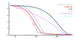
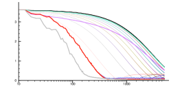
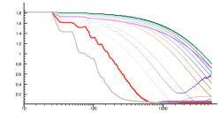
Error

Refer to caption Refer to caption Refer to caption

ฮป๐œ†\lambda value

Refer to caption Refer to caption Refer to caption
Chain 10 Chain 25 Chain 50
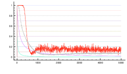
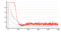
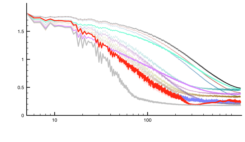
Figure 1: On-policy learning performance of GTD(ฮป๐œ†\lambda) with different methods of adapting ฮป๐œ†\lambda, for three sizes in the ringworld domain. The first row of results plots the mean squared value error verses time for several approaches to adapting ฮป๐œ†\lambda: the optimal ฮป๐œ†\lambda-greedy algorithm, our approximation algorithm, several fixed values of ฮป๐œ†\lambda, and two fixed decay schedules. The second row of results plots the ฮป๐œ†\lambda values over-time used by each algorithm. We highlight early learning by taking the log of y axis, as the algorithms should be able to exploit the low variance to learn quickly. For off-policy learning, there is more variance due to importance sampling and so we prefer long-term stability. We therefore highlight later learning using the log of the x-axis.

Error

Refer to caption Refer to caption

ฮป๐œ†\lambda value

Refer to caption Refer to caption
ฯ€โ€‹(s,right)=0.95,ฮผโ€‹(s,right)=0.85formulae-sequence๐œ‹๐‘ right0.95๐œ‡๐‘ right0.85\pi(s,\text{right})=0.95,\mu(s,\text{right})=0.85 ฯ€โ€‹(s,right)=0.95,ฮผโ€‹(s,right)=0.75formulae-sequence๐œ‹๐‘ right0.95๐œ‡๐‘ right0.75\pi(s,\text{right})=0.95,\mu(s,\text{right})=0.75
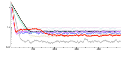
Figure 2: Off-policy learning performance of GTD(ฮป๐œ†\lambda) with different methods of adapting ฮป๐œ†\lambda, for two different configurations of ฯ€๐œ‹\pi and ฮผ๐œ‡\mu in the size 10 ringworld domain. The first row of results plots the mean squared value error verses time for several approaches to adapting ฮป๐œ†\lambda. In off-policy learning, there is more variance due to importance sampling and so we prefer long-term stability. We therefore highlight later learning using the log of the x-axis. The second row of results plots the ฮป๐œ†\lambda values over-time used by each algorithm.
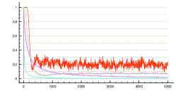
Refer to caption
Refer to caption
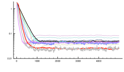
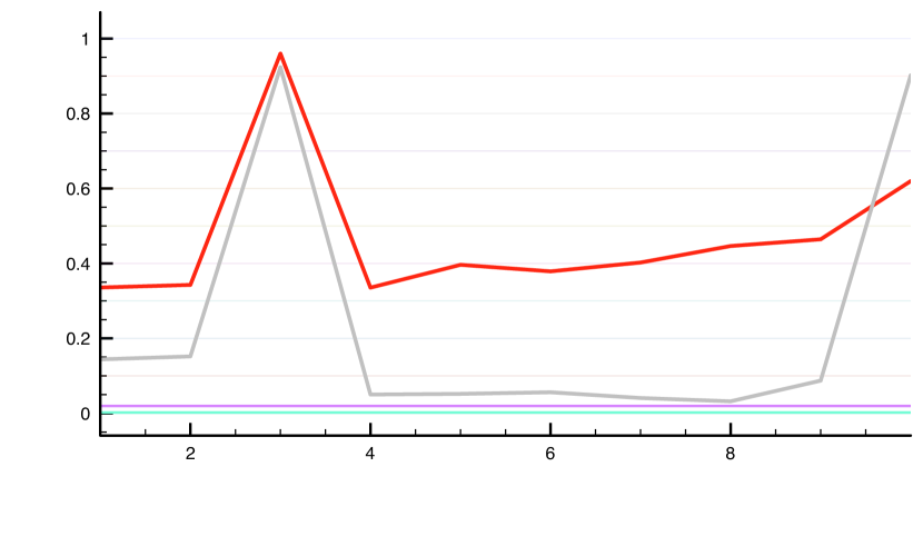
Figure 3: A closer examination of the effects of state aliasing on the choice of state-based ฮป๐œ†\lambda, for the length 10 chain with ฮณ=0.95๐›พ0.95\gamma=0.95, under on-policy sampling. State three is aliased with the last state. The left graph shows the learning curves over 5000 steps, and the right graph shows the learned ฮป๐œ†\lambda function in each state at the end of the run.

We investigate ฮป๐œ†\lambda-greedyย in a ring-world, under both on and off-policy sampling. This ring-world was previously introduced as a suitable domain for investigating ฮป๐œ†\lambda kearns2000bias . We varied the length of the ring-world from N=10,25,50๐‘102550N=10,25,50. The reward is zero in every state, except for two adjoining states that have +1 and -1 reward, and are terminal states. The agent is teleported back to the middle of the ring-world upon termination. The target policy is to take action โ€œrightโ€ with 95% probability, and action โ€œleftโ€ with 5% probability. The feature representation is a tabular encoding of states with binary identity vectors, but we also examine the effects of aliasing state values to simulate poor generalization: a common case where the true value function cannot be represented. The length of the experiment is a function of the problem size, Nร—100๐‘100N\times 100, proportionally scaling the number of samples for longer problem instances.

We compared to fixed values of ฮป=0,0.1,โ€ฆ,0.9,1.0๐œ†00.1โ€ฆ0.91.0\lambda=0,0.1,\ldots,0.9,1.0 and to two time-decay schedules, ฮปt=10/(10+t),ฮปt=100/(100+t)formulae-sequencesubscript๐œ†๐‘ก1010๐‘กsubscript๐œ†๐‘ก100100๐‘ก\lambda_{t}=10/(10+t),\lambda_{t}=100/(100+t), which worked well compared to several other tested settings. The discount factor is ฮณ=0.99๐›พ0.99\gamma=0.99 for the on-policy chains and 0.95 for the off-policy chains. We include the optimal ฮป๐œ†\lambda-greedy, which computes ๐ฐsqsuperscript๐ฐsq\mathbf{w}^{\text{sq}} and ๐ฐsqsuperscript๐ฐsq\mathbf{w}^{\text{sq}} using closed form solutions, defined by their respective Bellman operators. For ฮป๐œ†\lambda-greedy, the initialization was ๐ฐsq=0.0superscript๐ฐsq0.0\mathbf{w}^{\text{sq}}=0.0 and ๐ฐerr=Rโ€‹mโ€‹aโ€‹x1โˆ’ฮณร—๐Ÿsuperscript๐ฐerr๐‘…๐‘š๐‘Ž๐‘ฅ1๐›พ1\mathbf{w}^{\text{err}}=\frac{Rmax}{1-\gamma}\times\mathbf{\bm{1}} for on-policy, to match the rule-of-thumb of initializing with high lambdas, and the opposite for off-policy, to match the rule-of-thumb of more caution in off-policy domains. This max return value is a common choice for optimistic initialization, and prevented inadvertent evaluator bias by overly tuning this parameter. We fixed the learning-rate parameter for ฮป๐œ†\lambda-greedyย to be equal to equal to ฮฑ๐›ผ\alpha used in learning the value function (๐ฐ๐ฐ\mathbf{w}), again to demonstrate performance in less than ideal settings. Sweeping the step-size for ฮป๐œ†\lambda-greedyย would improve performance.

The performance results in on and off-policy are summarized in Figure 1 and 2. We report the absolute value error compared to the true value function, which is computable in this domain for each of the settings. We average over 100 runs, and report the results for the best parameter settings for each of the algorithms with 12 values of ฮฑโˆˆ{0.1ร—2j|j=โˆ’6,โˆ’6,โ€ฆ,5,6}๐›ผconditional-set0.1superscript2๐‘—๐‘—66โ€ฆ56\alpha\in\{0.1\times 2^{j}|j=-6,-6,...,5,6\}, 11 values of ฮทโˆˆ{2j|j=โˆ’16,โˆ’8,โˆ’4,โ€ฆ,4,8,16}๐œ‚conditional-setsuperscript2๐‘—๐‘—1684โ€ฆ4816\eta\in\{2^{j}|j=-16,-8,-4,\ldots,4,8,16\} (ฮฑ๐ก=ฮฑโ€‹ฮทsubscript๐›ผ๐ก๐›ผ๐œ‚\alpha_{\mathbf{h}}=\alpha\eta).

In general, we find that ฮป๐œ†\lambda-greedyย works well across settings. The optimal ฮป๐œ†\lambda-greedyย consistently performs the best, indicating the merit of the objective. Estimating ๐ฐsqsuperscript๐ฐsq\mathbf{w}^{\text{sq}} and ๐ฐsqsuperscript๐ฐsq\mathbf{w}^{\text{sq}} typically cause ฮป๐œ†\lambda-greedyย to perform more poorly, indicating an opportunity to improve these algorithms to match the performance of the optimal, idealistic version. In particular, we did not optimize the meta-parameters in ฮป๐œ†\lambda-greedy. For the fixed values of ฮป๐œ†\lambda and decay schedules, we find that they can be effective for specific instances, but do not perform well across problem settings. In particular, the fixed decay schedules settings appear to be un-robust to an increasing chain length and the fixed ฮป๐œ†\lambda are not robust to the change from on-policy to off-policy.

We also examined the ฮป๐œ†\lambda value selected by our ฮป๐œ†\lambda-greedyย algorithm plotted against time. For tabular features, ฮป๐œ†\lambda should converge to zero over-time, since the value function can be approximated and so, at some point, no bias is introduced by using ฮปt=0subscript๐œ†๐‘ก0\lambda_{t}=0, but variance is reduced. The algorithm does converge to a state-based ฮป๐œ†\lambda (ฮปโ€‹(s)โ‰ˆ0๐œ†๐‘ 0\lambda(s)\approx 0 for all states), which was one of our goals to ensure we have a well-defined fixed point. Second, for aliased features, we expect that the final per-state ฮป๐œ†\lambda should be larger for the states that have been aliased. The intuition is that one should not bootstrap on the values of these states, as that introduces bias. We demonstrate that this does indeed occur, in Figure 3. As expected, the ฮป๐œ†\lambda-greedyย is more robust to state aliasing, compared to the fixed strategies. State aliasing provides a concrete example of when we have less confidence in v^^๐‘ฃ\hat{v} in specific states, and an effective strategy to mitigate this situation is to set ฮป๐œ†\lambda high in those states.

8 Conclusion and discussion

In this paper, we have proposed the first linear-complexity ฮป๐œ†\lambda adaptation algorithm for incremental, off-policy reinforcement learning. We proposed an objective to greedily trade-off bias and variance, and derived an efficient algorithm to obtain the solution to this objective. We demonstrate the efficacy of the approach in an on-policy and off-policy setting, versus fixed values of ฮป๐œ†\lambda and time-decay heuristics.

This work opens up many avenues for efficiently selecting ฮป๐œ†\lambda, by providing a concrete greedy objective. One important direction is to extend the above analysis to use the recently introduced true-online traces vanseijen2014true ; here we focused on the more well-understood ฮป๐œ†\lambda-return, but the proposed objective is not restricted to that setting. There are also numerous future directions for improving optimization of this objective. We used GTD(ฮป=1๐œ†1\lambda=1) to learn the second moment of the ฮป๐œ†\lambda-return inside ฮป๐œ†\lambda-greedy. Another possible direction is to simply explore using ฮป<1๐œ†1\lambda<1 or even least-squares methods to improve estimation inside ฮป๐œ†\lambda-greedy.

There are also opportunities to modify the objective to consider variance into the future differently. The current objective is highly cautious, in that it assumes that only ฮปt+1subscript๐œ†๐‘ก1\lambda_{t+1} can be modified, and assumes the agent will be forced to use the unbiased ฮปt+i=1subscript๐œ†๐‘ก๐‘–1\lambda_{t+i}=1 for all future time steps. As a consequence, the algorithm will often prefer to set ฮปt+1subscript๐œ†๐‘ก1\lambda_{t+1} small, as future variance can only be controlled by the setting of ฮปt+1subscript๐œ†๐‘ก1\lambda_{t+1}. A natural relaxation of this strictly greedy setting is to recognize that the agent, in fact, has control over all future ฮปt+i,i>1subscript๐œ†๐‘ก๐‘–๐‘–1\lambda_{t+i},i>1. The agent could remain cautious for some number of steps, assuming ฮปt+isubscript๐œ†๐‘ก๐‘–\lambda_{t+i} will likely be high for 1<iโ‰คk1๐‘–๐‘˜1<i\leq k for some horizon k๐‘˜k. However, we can assume that after k๐‘˜k steps, ฮปt+isubscript๐œ†๐‘ก๐‘–\lambda_{t+i} we be reduced to a small value, cutting off the traces and mitigating the variance. The horizon k๐‘˜k could be encoded with an aggressive discount; multiplying the current discount ฮณยฏt+1subscriptยฏ๐›พ๐‘ก1\bar{\gamma}_{t+1} by a value less than 1. Commonly, a multiplicative factor less than 1 indicates a horizon of 11โˆ’factor11factor\frac{1}{1-\text{factor}}; for example, 11โˆ’0.8=5110.85\frac{1}{1-0.8}=5 gives a horizon of k=5๐‘˜5k=5. The variance term in the objective in (2) could be modified to include this horizon, providing a method to incorporate the level of caution.

Overall, this work takes a small step toward the goal of automatically selecting the trace parameter, and thus one step closer toward parameter-free black-box application of reinforcement learning with many avenues for future research.
Acknowledgements
We would like to thank David Silver for helpful discussions and the reviewers for helpful comments.

References

  • [1] P.ย L. A and M.ย Ghavamzadeh. Actor-Critic algorithms for risk-sensitive MDPs. In Advances in Neural Information Processing Systems, 2013.
  • [2] W.ย Dabney and A.ย G. Barto. Adaptive step-size for online temporal difference learning. In AAAI, 2012.
  • [3] C.ย Downey and S.ย Sanner. Temporal difference Bayesian model averaging: A Bayesian perspective on adapting lambda. In International Conference on Machine Learning, 2010.
  • [4] F.ย Garcia and F.ย Serre. From Q(lambda) to Average Q-learning: Efficient Implementation of an Asymptotic Approximation. In International Joint Conference on Artificial Intelligence, 2001.
  • [5] M.ย J. Kearns and S.ย P. Singh. Bias-Variance error bounds for temporal difference updates. In Annual Conference on Learning Theory, 2000.
  • [6] G.ย Konidaris, S.ย Niekum, and P.ย S. Thomas. TDgamma: Re-evaluating Complex Backups in Temporal Difference Learning. In NIPS, 2011.
  • [7] L.ย Li. A worst-case comparison between temporal difference and residual gradient with linear function approximation. In International Conference on Machine Learning, 2008.
  • [8] L.-J. Lin. Self-Improving Reactive Agents Based On Reinforcement Learning, Planning and Teaching. Machine Learning, 1992.
  • [9] H.ย Maei. Gradient Temporal-Difference Learning Algorithms. PhD thesis, University of Alberta, 2011.
  • [10] H.ย Maei and R.ย Sutton. GQ (ฮป๐œ†\lambda): A general gradient algorithm for temporal-difference prediction learning with eligibility traces. In AGI, 2010.
  • [11] A.ย R. Mahmood, H.ย P. van Hasselt, and R.ย S. Sutton. Weighted importance sampling for off-policy learning with linear function approximation. In Advances in Neural Information Processing Systems, 2014.
  • [12] S.ย Mannor, D.ย Simester, P.ย Sun, and J.ย N. Tsitsiklis. Bias and variance in value function estimation. In International Conference on Machine Learning, 2004.
  • [13] S.ย Mannor and J.ย N. Tsitsiklis. Mean-Variance pptimization in Markov Decision Processes. In ICML, 2011.
  • [14] J.ย Modayil, A.ย White, and R.ย S. Sutton. Multi-timescale nexting in a reinforcement learning robot. Adaptive Behavior - Animals, Animats, Software Agents, Robots, Adaptive Systems, 2014.
  • [15] T.ย Morimura, M.ย Sugiyama, H.ย Kashima, H.ย Hachiya, and T.ย Tanaka. Parametric return density estimation for reinforcement learning. In Conference on Uncertainty in Artificial Intelligence, 2010.
  • [16] A.ย L. Samuel. Some studies in machine learning using the game of checkers. IBM Journal of Research and Development (), 1959.
  • [17] R.ย E. Schapire and M.ย K. Warmuth. On the worst-case analysis of temporal-difference learning algorithms. Machine Learning, 1996.
  • [18] S.ย P. Singh and P.ย Dayan. Analytical mean squared error curves in temporal difference learning. In Advances in Neural Information Processing Systems, 1996.
  • [19] S.ย P. Singh and R.ย S. Sutton. Reinforcement learning with replacing eligibility traces. Machine Learning, 1996.
  • [20] M.ย J. Sobel. The variance of discounted Markov Decision Processes. Journal of Applied Probability, 1982.
  • [21] R.ย Sutton. Learning to predict by the methods of temporal differences. Machine Learning, 1988.
  • [22] R.ย Sutton. TD models: Modeling the world at a mixture of time scales. In International Conference on Machine Learning, 1995.
  • [23] R.ย Sutton and A.ย G. Barto. Introduction to reinforcement learning. MIT Press, 1998.
  • [24] R.ย Sutton, H.ย Maei, D.ย Precup, and S.ย Bhatnagar. Fast gradient-descent methods for temporal-difference learning with linear function approximation. International Conference on Machine Learning, 2009.
  • [25] R.ย Sutton and S.ย P. Singh. On step-size and bias in temporal-difference learning. In Proceedings of the Eighth Yale Workshop on Adaptive and Learning Systems, 1994.
  • [26] R.ย S. Sutton, A.ย R. Mahmood, and M.ย White. An emphatic approach to the problem of off-policy temporal-difference learning. The Journal of Machine Learning Research, 2015.
  • [27] R.ย S. Sutton, D.ย Precup, and S.ย Singh. Between MDPs and semi-MDPs: A framework for temporal abstraction in reinforcement learning. Artificial intelligence, 1999.
  • [28] A.ย Tamar, D.ย Diย Castro, and S.ย Mannor. Temporal difference methods for the variance of the reward to go. In International Conference on Machine Learning, 2013.
  • [29] G.ย Tesauro. Practical issues in temporal difference learning. Machine Learning, 1992.
  • [30] J.ย N. Tsitsiklis and B.ย Vanย Roy. An analysis of temporal-difference learning with function approximation. Automatic Control, IEEE Transactions on, 42(5):674โ€“690, 1997.
  • [31] H.ย van Hasselt, A.ย R. Mahmood, and R.ย Sutton. Off-policy TD (ฮป๐œ†\lambda) with a true online equivalence. In Conference on Uncertainty in Artificial Intelligence, 2014.
  • [32] H.ย van Seijen and R.ย Sutton. True online TD(lambda). In International Conference on Machine Learning, 2014.
  • [33] A.ย White. Developing a predictive approach to knowledge. PhD thesis, University of Alberta, 2015.
  • [34] M.ย White. Transition-based discounting in Markov decision processes. In preparation, 2016.
  • [35] M.ย White and A.ย White. Interval estimation for reinforcement-learning algorithms in continuous-state domains. In Advances in Neural Information Processing Systems, 2010.

Recall that for squared return (Gtฮป)2superscriptsubscriptsuperscript๐บ๐œ†๐‘ก2(G^{\lambda}_{t})^{2}, we use Vยฏtฮปยฏsubscriptsuperscriptยฏ๐‘‰ยฏ๐œ†๐‘ก\bar{V}^{\bar{\lambda}}_{t} to indicate the ฮปยฏยฏ๐œ†\bar{\lambda}-squared-return.

Vยฏtฮปยฏsubscriptsuperscriptยฏ๐‘‰ยฏ๐œ†๐‘ก\displaystyle\bar{V}^{\bar{\lambda}}_{t} =defโ€‹rยฏt+1+ฮณยฏt+1โ€‹((1โˆ’ฮปยฏt+1)โ€‹๐ฑt+1โŠคโ€‹๐ฐsq+ฮปยฏt+1โ€‹Vยฏt+1ฮปยฏ)defsubscriptยฏ๐‘Ÿ๐‘ก1subscriptยฏ๐›พ๐‘ก11subscriptยฏ๐œ†๐‘ก1superscriptsubscript๐ฑ๐‘ก1topsuperscript๐ฐsqsubscriptยฏ๐œ†๐‘ก1subscriptsuperscriptยฏ๐‘‰ยฏ๐œ†๐‘ก1\displaystyle\overset{\text{def}}{=}\bar{r}_{t+1}+\bar{\gamma}_{t+1}\left((1-\bar{\lambda}_{t+1})\mathbf{x}_{t+1}^{\top}\mathbf{w}^{\text{sq}}+\bar{\lambda}_{t+1}\bar{V}^{\bar{\lambda}}_{t+1}\right)
ฮดยฏtฮปยฏsubscriptsuperscriptยฏ๐›ฟยฏ๐œ†๐‘ก\displaystyle\bar{\delta}^{\bar{\lambda}}_{t} =defโ€‹Vยฏtฮปยฏโˆ’๐ฑtโŠคโ€‹๐ฐsqdefsubscriptsuperscriptยฏ๐‘‰ยฏ๐œ†๐‘กsuperscriptsubscript๐ฑ๐‘กtopsuperscript๐ฐsq\displaystyle\overset{\text{def}}{=}\bar{V}^{\bar{\lambda}}_{t}-\mathbf{x}_{t}^{\top}\mathbf{w}^{\text{sq}}
ฮดยฏtsubscriptยฏ๐›ฟ๐‘ก\displaystyle\bar{\delta}_{t} =defโ€‹rยฏt+1+ฮณยฏt+1โ€‹๐ฑt+1โŠคโ€‹๐ฐsqโˆ’๐ฑtโŠคโ€‹๐ฐsqdefsubscriptยฏ๐‘Ÿ๐‘ก1subscriptยฏ๐›พ๐‘ก1superscriptsubscript๐ฑ๐‘ก1topsuperscript๐ฐsqsuperscriptsubscript๐ฑ๐‘กtopsuperscript๐ฐsq\displaystyle\overset{\text{def}}{=}\bar{r}_{t+1}+\bar{\gamma}_{t+1}\mathbf{x}_{t+1}^{\top}\mathbf{w}^{\text{sq}}-\mathbf{x}_{t}^{\top}\mathbf{w}^{\text{sq}}
rยฏt+1subscriptยฏ๐‘Ÿ๐‘ก1\displaystyle\bar{r}_{t+1} =defโ€‹ฯt2โ€‹Gยฏt2+2โ€‹ฯt2โ€‹ฮณt+1โ€‹ฮปt+1โ€‹Gยฏtโ€‹Gt+1ฮปdefsuperscriptsubscript๐œŒ๐‘ก2superscriptsubscriptยฏ๐บ๐‘ก22superscriptsubscript๐œŒ๐‘ก2subscript๐›พ๐‘ก1subscript๐œ†๐‘ก1subscriptยฏ๐บ๐‘กsubscriptsuperscript๐บ๐œ†๐‘ก1\displaystyle\overset{\text{def}}{=}\rho_{t}^{2}\bar{G}_{t}^{2}+2\rho_{t}^{2}\gamma_{t+1}\lambda_{t+1}\bar{G}_{t}{G^{\lambda}_{t+1}}
ฮณยฏt+1subscriptยฏ๐›พ๐‘ก1\displaystyle\bar{\gamma}_{t+1} =defโ€‹ฯt2โ€‹ฮณt+12โ€‹ฮปt+12defsuperscriptsubscript๐œŒ๐‘ก2superscriptsubscript๐›พ๐‘ก12superscriptsubscript๐œ†๐‘ก12\displaystyle\overset{\text{def}}{=}\rho_{t}^{2}\gamma_{t+1}^{2}\lambda_{t+1}^{2}
Gยฏtsubscriptยฏ๐บ๐‘ก\displaystyle\bar{G}_{t} =defโ€‹Rt+1+ฮณt+1โ€‹(1โˆ’ฮปt+1)โ€‹๐ฑt+1โŠคโ€‹๐ฐ.defsubscript๐‘…๐‘ก1subscript๐›พ๐‘ก11subscript๐œ†๐‘ก1superscriptsubscript๐ฑ๐‘ก1top๐ฐ\displaystyle\overset{\text{def}}{=}R_{t+1}+\gamma_{t+1}(1-\lambda_{t+1})\mathbf{x}_{t+1}^{\top}\mathbf{w}.

If ฮปยฏ=1ยฏ๐œ†1\bar{\lambda}=1, then Vยฏtฮปยฏ=(Gtฮป)2subscriptsuperscriptยฏ๐‘‰ยฏ๐œ†๐‘กsuperscriptsubscriptsuperscript๐บ๐œ†๐‘ก2\bar{V}^{\bar{\lambda}}_{t}=(G^{\lambda}_{t})^{2}. Note that the weights ๐ฐ๐ฐ\mathbf{w} in Gยฏtsubscriptยฏ๐บ๐‘ก\bar{G}_{t} are the weights for the main estimator that defines the ฮป๐œ†\lambda-return, not the weights ๐ฐsqsuperscript๐ฐsq\mathbf{w}^{\text{sq}} that estimate the second moment of the ฮป๐œ†\lambda-return.

Theorem 1 For a given ฮปยฏ:๐’ฎโ†’[0,1]:ยฏ๐œ†โ†’๐’ฎ01\bar{\lambda}:\mathcal{S}\rightarrow[0,1],

๐”ผโ€‹[ฮดยฏtฮปยฏโ€‹๐ฑt]๐”ผdelimited-[]subscriptsuperscriptยฏ๐›ฟยฏ๐œ†๐‘กsubscript๐ฑ๐‘ก\displaystyle\mathbb{E}[\bar{\delta}^{\bar{\lambda}}_{t}\mathbf{x}_{t}] =๐”ผโ€‹[ฮดยฏtโ€‹๐ณยฏt]absent๐”ผdelimited-[]subscriptยฏ๐›ฟ๐‘กsubscriptยฏ๐ณ๐‘ก\displaystyle=\mathbb{E}[\bar{\delta}_{t}\mathbf{\bar{z}}_{t}]

where

๐ณยฏtsubscriptยฏ๐ณ๐‘ก\displaystyle{\bar{\mathbf{z}}_{t}} =defโ€‹๐ฑt+ฮณยฏtโ€‹ฮปยฏtโ€‹๐ณยฏtโˆ’1defsubscript๐ฑ๐‘กsubscriptยฏ๐›พ๐‘กsubscriptยฏ๐œ†๐‘กsubscriptยฏ๐ณ๐‘ก1\displaystyle\overset{\text{def}}{=}\mathbf{x}_{t}+\bar{\gamma}_{t}\bar{\lambda}_{t}{\bar{\mathbf{z}}_{t-1}}
Proof

As in other TD algorithms [9], we use index shifting to obtain an unbiased estimate of future values using traces.

Vยฏtฮปยฏsubscriptsuperscriptยฏ๐‘‰ยฏ๐œ†๐‘ก\displaystyle\bar{V}^{\bar{\lambda}}_{t} =rยฏt+1+ฮณยฏt+1โ€‹((1โˆ’ฮปยฏt+1)โ€‹๐ฑt+1โŠคโ€‹๐ฐsq+ฮปยฏt+1โ€‹Vยฏt+1ฮปยฏ)absentsubscriptยฏ๐‘Ÿ๐‘ก1subscriptยฏ๐›พ๐‘ก11subscriptยฏ๐œ†๐‘ก1superscriptsubscript๐ฑ๐‘ก1topsuperscript๐ฐsqsubscriptยฏ๐œ†๐‘ก1subscriptsuperscriptยฏ๐‘‰ยฏ๐œ†๐‘ก1\displaystyle=\bar{r}_{t+1}+\bar{\gamma}_{t+1}\left((1-\bar{\lambda}_{t+1})\mathbf{x}_{t+1}^{\top}\mathbf{w}^{\text{sq}}+\bar{\lambda}_{t+1}\bar{V}^{\bar{\lambda}}_{t+1}\right)
=rยฏt+1+ฮณยฏt+1โ€‹๐ฑt+1โŠคโ€‹๐ฐsqโˆ’ฮณยฏt+1โ€‹ฮปยฏt+1โ€‹๐ฑt+1โŠคโ€‹๐ฐsq+ฮณยฏt+1โ€‹ฮปยฏt+1โ€‹Vยฏt+1ฮปยฏabsentsubscriptยฏ๐‘Ÿ๐‘ก1subscriptยฏ๐›พ๐‘ก1superscriptsubscript๐ฑ๐‘ก1topsuperscript๐ฐsqsubscriptยฏ๐›พ๐‘ก1subscriptยฏ๐œ†๐‘ก1superscriptsubscript๐ฑ๐‘ก1topsuperscript๐ฐsqsubscriptยฏ๐›พ๐‘ก1subscriptยฏ๐œ†๐‘ก1subscriptsuperscriptยฏ๐‘‰ยฏ๐œ†๐‘ก1\displaystyle=\bar{r}_{t+1}+\bar{\gamma}_{t+1}\mathbf{x}_{t+1}^{\top}\mathbf{w}^{\text{sq}}-\bar{\gamma}_{t+1}\bar{\lambda}_{t+1}\mathbf{x}_{t+1}^{\top}\mathbf{w}^{\text{sq}}+\bar{\gamma}_{t+1}\bar{\lambda}_{t+1}\bar{V}^{\bar{\lambda}}_{t+1}
=rยฏt+1+ฮณยฏt+1โ€‹๐ฑt+1โŠคโ€‹๐ฐsq+ฮณยฏt+1โ€‹ฮปยฏt+1โ€‹ฮดยฏt+1ฮปยฏabsentsubscriptยฏ๐‘Ÿ๐‘ก1subscriptยฏ๐›พ๐‘ก1superscriptsubscript๐ฑ๐‘ก1topsuperscript๐ฐsqsubscriptยฏ๐›พ๐‘ก1subscriptยฏ๐œ†๐‘ก1subscriptsuperscriptยฏ๐›ฟยฏ๐œ†๐‘ก1\displaystyle=\bar{r}_{t+1}+\bar{\gamma}_{t+1}\mathbf{x}_{t+1}^{\top}\mathbf{w}^{\text{sq}}+\bar{\gamma}_{t+1}\bar{\lambda}_{t+1}\bar{\delta}^{\bar{\lambda}}_{t+1}

Therefore, for ฮดยฏt=rยฏt+1+ฮณยฏt+1โ€‹๐ฑt+1โŠคโ€‹๐ฐsqโˆ’๐ฑtโŠคโ€‹๐ฐsqsubscriptยฏ๐›ฟ๐‘กsubscriptยฏ๐‘Ÿ๐‘ก1subscriptยฏ๐›พ๐‘ก1superscriptsubscript๐ฑ๐‘ก1topsuperscript๐ฐsqsuperscriptsubscript๐ฑ๐‘กtopsuperscript๐ฐsq\bar{\delta}_{t}=\bar{r}_{t+1}+\bar{\gamma}_{t+1}\mathbf{x}_{t+1}^{\top}\mathbf{w}^{\text{sq}}-\mathbf{x}_{t}^{\top}\mathbf{w}^{\text{sq}},

๐”ผโ€‹[ฮดยฏtฮปยฏโ€‹๐ฑt]๐”ผdelimited-[]subscriptsuperscriptยฏ๐›ฟยฏ๐œ†๐‘กsubscript๐ฑ๐‘ก\displaystyle\mathbb{E}[\bar{\delta}^{\bar{\lambda}}_{t}\mathbf{x}_{t}] =๐”ผโ€‹[(Vยฏtฮปยฏโˆ’๐ฑtโŠคโ€‹๐ฐsq)โ€‹๐ฑt]absent๐”ผdelimited-[]subscriptsuperscriptยฏ๐‘‰ยฏ๐œ†๐‘กsuperscriptsubscript๐ฑ๐‘กtopsuperscript๐ฐsqsubscript๐ฑ๐‘ก\displaystyle=\mathbb{E}[(\bar{V}^{\bar{\lambda}}_{t}-\mathbf{x}_{t}^{\top}\mathbf{w}^{\text{sq}})\mathbf{x}_{t}]
=๐”ผโ€‹[(ฮดยฏt+ฮณยฏt+1โ€‹ฮปยฏt+1โ€‹ฮดยฏt+1ฮปยฏ)โ€‹๐ฑt]absent๐”ผdelimited-[]subscriptยฏ๐›ฟ๐‘กsubscriptยฏ๐›พ๐‘ก1subscriptยฏ๐œ†๐‘ก1subscriptsuperscriptยฏ๐›ฟยฏ๐œ†๐‘ก1subscript๐ฑ๐‘ก\displaystyle=\mathbb{E}[(\bar{\delta}_{t}+\bar{\gamma}_{t+1}\bar{\lambda}_{t+1}\bar{\delta}^{\bar{\lambda}}_{t+1})\mathbf{x}_{t}]
=๐”ผโ€‹[ฮดยฏtโ€‹๐ฑt]+๐”ผโ€‹[ฮณยฏtโ€‹ฮปยฏtโ€‹ฮดยฏtฮปยฏโ€‹๐ฑtโˆ’1]absent๐”ผdelimited-[]subscriptยฏ๐›ฟ๐‘กsubscript๐ฑ๐‘ก๐”ผdelimited-[]subscriptยฏ๐›พ๐‘กsubscriptยฏ๐œ†๐‘กsubscriptsuperscriptยฏ๐›ฟยฏ๐œ†๐‘กsubscript๐ฑ๐‘ก1\displaystyle=\mathbb{E}[\bar{\delta}_{t}\mathbf{x}_{t}]+\mathbb{E}[\bar{\gamma}_{t}\bar{\lambda}_{t}\bar{\delta}^{\bar{\lambda}}_{t}\mathbf{x}_{t-1}]
=๐”ผโ€‹[ฮดยฏtโ€‹๐ฑt]+๐”ผโ€‹[ฮณยฏtโ€‹ฮปยฏtโ€‹(ฮดยฏt+ฮณยฏt+1โ€‹ฮปยฏt+1โ€‹ฮดยฏt+1ฮปยฏ)โ€‹๐ฑtโˆ’1]absent๐”ผdelimited-[]subscriptยฏ๐›ฟ๐‘กsubscript๐ฑ๐‘ก๐”ผdelimited-[]subscriptยฏ๐›พ๐‘กsubscriptยฏ๐œ†๐‘กsubscriptยฏ๐›ฟ๐‘กsubscriptยฏ๐›พ๐‘ก1subscriptยฏ๐œ†๐‘ก1subscriptsuperscriptยฏ๐›ฟยฏ๐œ†๐‘ก1subscript๐ฑ๐‘ก1\displaystyle=\mathbb{E}[\bar{\delta}_{t}\mathbf{x}_{t}]+\mathbb{E}[\bar{\gamma}_{t}\bar{\lambda}_{t}(\bar{\delta}_{t}+\bar{\gamma}_{t+1}\bar{\lambda}_{t+1}\bar{\delta}^{\bar{\lambda}}_{t+1})\mathbf{x}_{t-1}]
=๐”ผโ€‹[ฮดยฏtโ€‹(๐ฑt+ฮณยฏtโ€‹ฮปยฏtโ€‹๐ฑtโˆ’1)]+๐”ผโ€‹[ฮณยฏtโ€‹ฮปยฏtโ€‹ฮณยฏt+1โ€‹ฮปยฏt+1โ€‹ฮดยฏt+1ฮปยฏโ€‹๐ฑtโˆ’1]absent๐”ผdelimited-[]subscriptยฏ๐›ฟ๐‘กsubscript๐ฑ๐‘กsubscriptยฏ๐›พ๐‘กsubscriptยฏ๐œ†๐‘กsubscript๐ฑ๐‘ก1๐”ผdelimited-[]subscriptยฏ๐›พ๐‘กsubscriptยฏ๐œ†๐‘กsubscriptยฏ๐›พ๐‘ก1subscriptยฏ๐œ†๐‘ก1subscriptsuperscriptยฏ๐›ฟยฏ๐œ†๐‘ก1subscript๐ฑ๐‘ก1\displaystyle=\mathbb{E}[\bar{\delta}_{t}(\mathbf{x}_{t}+\bar{\gamma}_{t}\bar{\lambda}_{t}\mathbf{x}_{t-1})]+\mathbb{E}[\bar{\gamma}_{t}\bar{\lambda}_{t}\bar{\gamma}_{t+1}\bar{\lambda}_{t+1}\bar{\delta}^{\bar{\lambda}}_{t+1}\mathbf{x}_{t-1}]
=๐”ผโ€‹[ฮดยฏtโ€‹(๐ฑt+ฮณยฏtโ€‹ฮปยฏtโ€‹๐ฑtโˆ’1)]+๐”ผโ€‹[ฮณยฏtโˆ’1โ€‹ฮปยฏtโˆ’1โ€‹ฮณยฏtโ€‹ฮปยฏtโ€‹ฮดยฏtฮปยฏโ€‹๐ฑtโˆ’2]absent๐”ผdelimited-[]subscriptยฏ๐›ฟ๐‘กsubscript๐ฑ๐‘กsubscriptยฏ๐›พ๐‘กsubscriptยฏ๐œ†๐‘กsubscript๐ฑ๐‘ก1๐”ผdelimited-[]subscriptยฏ๐›พ๐‘ก1subscriptยฏ๐œ†๐‘ก1subscriptยฏ๐›พ๐‘กsubscriptยฏ๐œ†๐‘กsubscriptsuperscriptยฏ๐›ฟยฏ๐œ†๐‘กsubscript๐ฑ๐‘ก2\displaystyle=\mathbb{E}[\bar{\delta}_{t}(\mathbf{x}_{t}+\bar{\gamma}_{t}\bar{\lambda}_{t}\mathbf{x}_{t-1})]+\mathbb{E}[\bar{\gamma}_{t-1}\bar{\lambda}_{t-1}\bar{\gamma}_{t}\bar{\lambda}_{t}\bar{\delta}^{\bar{\lambda}}_{t}\mathbf{x}_{t-2}]
=โ€ฆabsentโ€ฆ\displaystyle=\ldots
=๐”ผโ€‹[ฮดยฏtโ€‹๐ณยฏt]absent๐”ผdelimited-[]subscriptยฏ๐›ฟ๐‘กsubscriptยฏ๐ณ๐‘ก\displaystyle=\mathbb{E}[\bar{\delta}_{t}\mathbf{\bar{z}}_{t}]

To enable the above recursive form, we need to ensure that rยฏt+1subscriptยฏ๐‘Ÿ๐‘ก1\bar{r}_{t+1} is computable on each step, given St,St+1subscript๐‘†๐‘กsubscript๐‘†๐‘ก1S_{t},S_{t+1}. We characterize the expectation of rยฏt+1subscriptยฏ๐‘Ÿ๐‘ก1\bar{r}_{t+1}, using the current unbiased estimate ๐ฑtโŠคโ€‹๐ฐerrsuperscriptsubscript๐ฑ๐‘กtopsuperscript๐ฐerr\mathbf{x}_{t}^{\top}\mathbf{w}^{\text{err}} of ๐”ผโ€‹[Gt+1ฮป|St+1]๐”ผdelimited-[]conditionalsubscriptsuperscript๐บ๐œ†๐‘ก1subscript๐‘†๐‘ก1\mathbb{E}[{G^{\lambda}_{t+1}}|S_{t+1}], providing a way to obtain an unbiased sample of rยฏt+1subscriptยฏ๐‘Ÿ๐‘ก1\bar{r}_{t+1} on each step.

Proposition 4
๐”ผโ€‹[rยฏt+1|St,St+1]๐”ผdelimited-[]conditionalsubscriptยฏ๐‘Ÿ๐‘ก1subscript๐‘†๐‘กsubscript๐‘†๐‘ก1\displaystyle\mathbb{E}[\bar{r}_{t+1}|S_{t},S_{t+1}] =๐”ผโ€‹[ฯt2โ€‹Gยฏt2|St,St+1]absent๐”ผdelimited-[]conditionalsuperscriptsubscript๐œŒ๐‘ก2superscriptsubscriptยฏ๐บ๐‘ก2subscript๐‘†๐‘กsubscript๐‘†๐‘ก1\displaystyle=\mathbb{E}[\rho_{t}^{2}\bar{G}_{t}^{2}|S_{t},S_{t+1}]
+2โ€‹๐”ผโ€‹[ฯt2โ€‹ฮณt+1โ€‹ฮปt+1โ€‹Gยฏt|St,St+1]โ€‹๐”ผโ€‹[Gt+1ฮป|St+1]2๐”ผdelimited-[]conditionalsuperscriptsubscript๐œŒ๐‘ก2subscript๐›พ๐‘ก1subscript๐œ†๐‘ก1subscriptยฏ๐บ๐‘กsubscript๐‘†๐‘กsubscript๐‘†๐‘ก1๐”ผdelimited-[]conditionalsubscriptsuperscript๐บ๐œ†๐‘ก1subscript๐‘†๐‘ก1\displaystyle+2\mathbb{E}[\rho_{t}^{2}\gamma_{t+1}\lambda_{t+1}\bar{G}_{t}|S_{t},S_{t+1}]\mathbb{E}[{G^{\lambda}_{t+1}}|S_{t+1}]
Proof
๐”ผโ€‹[rยฏt+1|St,St+1]๐”ผdelimited-[]conditionalsubscriptยฏ๐‘Ÿ๐‘ก1subscript๐‘†๐‘กsubscript๐‘†๐‘ก1\displaystyle\mathbb{E}[\bar{r}_{t+1}|S_{t},S_{t+1}] =๐”ผโ€‹[ฯt2โ€‹Gยฏt2+2โ€‹ฯt2โ€‹ฮณt+1โ€‹ฮปt+1โ€‹Gยฏtโ€‹Gt+1ฮป|St,St+1]absent๐”ผdelimited-[]superscriptsubscript๐œŒ๐‘ก2superscriptsubscriptยฏ๐บ๐‘ก2conditional2superscriptsubscript๐œŒ๐‘ก2subscript๐›พ๐‘ก1subscript๐œ†๐‘ก1subscriptยฏ๐บ๐‘กsubscriptsuperscript๐บ๐œ†๐‘ก1subscript๐‘†๐‘กsubscript๐‘†๐‘ก1\displaystyle=\mathbb{E}[\rho_{t}^{2}\bar{G}_{t}^{2}+2\rho_{t}^{2}\gamma_{t+1}\lambda_{t+1}\bar{G}_{t}{G^{\lambda}_{t+1}}|S_{t},S_{t+1}]
=๐”ผโ€‹[ฯt2โ€‹Gยฏt2|St,St+1]absent๐”ผdelimited-[]conditionalsuperscriptsubscript๐œŒ๐‘ก2superscriptsubscriptยฏ๐บ๐‘ก2subscript๐‘†๐‘กsubscript๐‘†๐‘ก1\displaystyle=\mathbb{E}[\rho_{t}^{2}\bar{G}_{t}^{2}|S_{t},S_{t+1}]
+2โ€‹๐”ผโ€‹[ฯt2โ€‹ฮณt+1โ€‹ฮปt+1|St,St+1]โ€‹๐”ผโ€‹[Gยฏtโ€‹Gt+1ฮป|St,St+1]2๐”ผdelimited-[]conditionalsuperscriptsubscript๐œŒ๐‘ก2subscript๐›พ๐‘ก1subscript๐œ†๐‘ก1subscript๐‘†๐‘กsubscript๐‘†๐‘ก1๐”ผdelimited-[]conditionalsubscriptยฏ๐บ๐‘กsubscriptsuperscript๐บ๐œ†๐‘ก1subscript๐‘†๐‘กsubscript๐‘†๐‘ก1\displaystyle+2\mathbb{E}[\rho_{t}^{2}\gamma_{t+1}\lambda_{t+1}|S_{t},S_{t+1}]\mathbb{E}[\bar{G}_{t}{G^{\lambda}_{t+1}}|S_{t},S_{t+1}]

Now because we assumed independent, zero-mean noise in the reward, i.e. Rt+1=๐”ผโ€‹[Rt+1|St,St+1]+ฯตt+1subscript๐‘…๐‘ก1๐”ผdelimited-[]conditionalsubscript๐‘…๐‘ก1subscript๐‘†๐‘กsubscript๐‘†๐‘ก1subscriptitalic-ฯต๐‘ก1R_{t+1}=\mathbb{E}[R_{t+1}|S_{t},S_{t+1}]+\epsilon_{t+1} for independent zero-mean noise ฯตt+1subscriptitalic-ฯต๐‘ก1\epsilon_{t+1}, because we assume that ๐ฑt+1subscript๐ฑ๐‘ก1\mathbf{x}_{t+1} is completely determined by St+1subscript๐‘†๐‘ก1S_{t+1} and because
๐”ผโ€‹[Gt+1ฮป|St,St+1]=๐”ผโ€‹[Gt+1ฮป|St+1]๐”ผdelimited-[]conditionalsubscriptsuperscript๐บ๐œ†๐‘ก1subscript๐‘†๐‘กsubscript๐‘†๐‘ก1๐”ผdelimited-[]conditionalsubscriptsuperscript๐บ๐œ†๐‘ก1subscript๐‘†๐‘ก1\mathbb{E}[{G^{\lambda}_{t+1}}|S_{t},S_{t+1}]=\mathbb{E}[{G^{\lambda}_{t+1}}|S_{t+1}], we obtain

๐”ผโ€‹[Gยฏtโ€‹Gt+1ฮป|St+1]๐”ผdelimited-[]conditionalsubscriptยฏ๐บ๐‘กsubscriptsuperscript๐บ๐œ†๐‘ก1subscript๐‘†๐‘ก1\displaystyle\mathbb{E}[\bar{G}_{t}{G^{\lambda}_{t+1}}|S_{t+1}]
=๐”ผโ€‹[(Rt+1+ฮณt+1โ€‹(1โˆ’ฮปt+1)โ€‹๐ฑt+1โŠคโ€‹๐ฐ)โ€‹Gt+1ฮป|St,St+1]absent๐”ผdelimited-[]conditionalsubscript๐‘…๐‘ก1subscript๐›พ๐‘ก11subscript๐œ†๐‘ก1superscriptsubscript๐ฑ๐‘ก1top๐ฐsubscriptsuperscript๐บ๐œ†๐‘ก1subscript๐‘†๐‘กsubscript๐‘†๐‘ก1\displaystyle=\mathbb{E}[(R_{t+1}+\gamma_{t+1}(1-\lambda_{t+1})\mathbf{x}_{t+1}^{\top}\mathbf{w}){G^{\lambda}_{t+1}}|S_{t},S_{t+1}]
=๐”ผโ€‹[Rt+1|St,St+1]โ€‹๐”ผโ€‹[Gt+1ฮป|St+1]absent๐”ผdelimited-[]conditionalsubscript๐‘…๐‘ก1subscript๐‘†๐‘กsubscript๐‘†๐‘ก1๐”ผdelimited-[]conditionalsubscriptsuperscript๐บ๐œ†๐‘ก1subscript๐‘†๐‘ก1\displaystyle=\mathbb{E}[R_{t+1}|S_{t},S_{t+1}]\mathbb{E}[{G^{\lambda}_{t+1}}|S_{t+1}]
+๐”ผโ€‹[ฮณt+1โ€‹(1โˆ’ฮปt+1)โ€‹๐ฑt+1โŠคโ€‹๐ฐ|St,St+1]โ€‹๐”ผโ€‹[Gt+1ฮป|St+1]๐”ผdelimited-[]conditionalsubscript๐›พ๐‘ก11subscript๐œ†๐‘ก1superscriptsubscript๐ฑ๐‘ก1top๐ฐsubscript๐‘†๐‘กsubscript๐‘†๐‘ก1๐”ผdelimited-[]conditionalsubscriptsuperscript๐บ๐œ†๐‘ก1subscript๐‘†๐‘ก1\displaystyle+\mathbb{E}[\gamma_{t+1}(1-\lambda_{t+1})\mathbf{x}_{t+1}^{\top}\mathbf{w}|S_{t},S_{t+1}]\mathbb{E}[{G^{\lambda}_{t+1}}|S_{t+1}]

completing the proof.

This previous result requires that rยฏt+1subscriptยฏ๐‘Ÿ๐‘ก1\bar{r}_{t+1} can be given to the algorithm on each step. The result in Theorem 1 requires an an estimate of ๐”ผโ€‹[Gt+1ฮป|St+1]๐”ผdelimited-[]conditionalsubscriptsuperscript๐บ๐œ†๐‘ก1subscript๐‘†๐‘ก1\mathbb{E}[{G^{\lambda}_{t+1}}|S_{t+1}], to define the reward; such an estimate, however, may not always be available. We characterize the expectation ๐”ผโ€‹[ฮดยฏtฮปยฏโ€‹๐ฑt]๐”ผdelimited-[]subscriptsuperscriptยฏ๐›ฟยฏ๐œ†๐‘กsubscript๐ฑ๐‘ก\mathbb{E}[\bar{\delta}^{\bar{\lambda}}_{t}\mathbf{x}_{t}] in the next theorem, when such an estimate is not provided. For general trace functions ฮป๐œ†\lambda, this estimate requires a matrix to be stored and updated; however, for ฮป=1๐œ†1\lambda=1 as addressed in this work, Corollary LABEL:corollary_mse indicates that this simplifies to a linear-space and time algorithm.

Theorem 2

๐”ผโ€‹[rยฏt+1โ€‹๐ณยฏt]=Eโ€‹[ฯt+12โ€‹Gยฏt2โ€‹๐ณยฏt]+2โ€‹Eโ€‹[ฯt+12โ€‹Gยฏtโ€‹(๐šยฏt+๐ยฏtโ€‹๐ฐt)]๐”ผdelimited-[]subscriptยฏ๐‘Ÿ๐‘ก1subscriptยฏ๐ณ๐‘ก๐ธdelimited-[]superscriptsubscript๐œŒ๐‘ก12superscriptsubscriptยฏ๐บ๐‘ก2subscriptยฏ๐ณ๐‘ก2๐ธdelimited-[]superscriptsubscript๐œŒ๐‘ก12subscriptยฏ๐บ๐‘กsubscriptยฏ๐š๐‘กsubscriptยฏ๐๐‘กsubscript๐ฐ๐‘ก\displaystyle\mathbb{E}[\bar{r}_{t+1}\mathbf{\bar{z}}_{t}]=E[\rho_{t+1}^{2}\bar{G}_{t}^{2}{\bar{\mathbf{z}}_{t}}]+2E[\rho_{t+1}^{2}\bar{G}_{t}({\bar{\mathbf{a}}_{t}}+{\bar{\mathbf{B}}_{t}}\mathbf{w}_{t})]

where

๐šยฏtsubscriptยฏ๐š๐‘ก\displaystyle{\bar{\mathbf{a}}_{t}} =defโ€‹ฯtโ€‹ฮณtโ€‹ฮปtโ€‹(Rtโ€‹๐ณยฏtโˆ’1+๐šยฏtโˆ’1)defsubscript๐œŒ๐‘กsubscript๐›พ๐‘กsubscript๐œ†๐‘กsubscript๐‘…๐‘กsubscriptยฏ๐ณ๐‘ก1subscriptยฏ๐š๐‘ก1\displaystyle\overset{\text{def}}{=}\rho_{t}\gamma_{t}\lambda_{t}(R_{t}{\bar{\mathbf{z}}_{t-1}}+{\bar{\mathbf{a}}_{t-1}})
๐ยฏtsubscriptยฏ๐๐‘ก\displaystyle{\bar{\mathbf{B}}_{t}} =defโ€‹ฯtโ€‹ฮณtโ€‹ฮปtโ€‹(ฮณtโ€‹(1โˆ’ฮปt)โ€‹๐ณยฏtโˆ’1โ€‹๐ฑtโŠค+๐ยฏtโˆ’1)defsubscript๐œŒ๐‘กsubscript๐›พ๐‘กsubscript๐œ†๐‘กsubscript๐›พ๐‘ก1subscript๐œ†๐‘กsubscriptยฏ๐ณ๐‘ก1superscriptsubscript๐ฑ๐‘กtopsubscriptยฏ๐๐‘ก1\displaystyle\overset{\text{def}}{=}\rho_{t}\gamma_{t}\lambda_{t}(\gamma_{t}(1-\lambda_{t}){\bar{\mathbf{z}}_{t-1}}\mathbf{x}_{t}^{\top}+{\bar{\mathbf{B}}_{t-1}})
Proof
๐”ผโ€‹[rยฏt+1โ€‹๐ณยฏt]=Eโ€‹[ฯt2โ€‹Gยฏt2โ€‹๐ณยฏt]+2โ€‹Eโ€‹[ฯt2โ€‹ฮณt+1โ€‹ฮปt+1โ€‹Gยฏtโ€‹Gt+1ฮปโ€‹๐ณยฏt]๐”ผdelimited-[]subscriptยฏ๐‘Ÿ๐‘ก1subscriptยฏ๐ณ๐‘ก๐ธdelimited-[]superscriptsubscript๐œŒ๐‘ก2superscriptsubscriptยฏ๐บ๐‘ก2subscriptยฏ๐ณ๐‘ก2๐ธdelimited-[]superscriptsubscript๐œŒ๐‘ก2subscript๐›พ๐‘ก1subscript๐œ†๐‘ก1subscriptยฏ๐บ๐‘กsubscriptsuperscript๐บ๐œ†๐‘ก1subscriptยฏ๐ณ๐‘ก\displaystyle\mathbb{E}[\bar{r}_{t+1}\mathbf{\bar{z}}_{t}]=E[\rho_{t}^{2}\bar{G}_{t}^{2}{\bar{\mathbf{z}}_{t}}]+2E[\rho_{t}^{2}\gamma_{t+1}\lambda_{t+1}\bar{G}_{t}{G^{\lambda}_{t+1}}\mathbf{\bar{z}}_{t}]

Now let us look at this second term which still contains Gtฮปsubscriptsuperscript๐บ๐œ†๐‘ก{G^{\lambda}_{t}}.

๐”ผโ€‹[ฮณtโ€‹ฮปtโ€‹Gtฮปโ€‹Gยฏtโˆ’1โ€‹ฯtโˆ’12โ€‹๐ณยฏtโˆ’1]๐”ผdelimited-[]subscript๐›พ๐‘กsubscript๐œ†๐‘กsubscriptsuperscript๐บ๐œ†๐‘กsubscriptยฏ๐บ๐‘ก1superscriptsubscript๐œŒ๐‘ก12subscriptยฏ๐ณ๐‘ก1\displaystyle\mathbb{E}[\gamma_{t}\lambda_{t}{G^{\lambda}_{t}}\bar{G}_{t-1}\rho_{t-1}^{2}{\bar{\mathbf{z}}_{t-1}}]
=๐”ผโ€‹[ฯtโ€‹ฮณtโ€‹ฮปtโ€‹(Gยฏt+ฮณt+1โ€‹ฮปt+1โ€‹Gt+1ฮป)โ€‹Gยฏtโˆ’1โ€‹ฯtโˆ’12โ€‹๐ณยฏtโˆ’1]absent๐”ผdelimited-[]subscript๐œŒ๐‘กsubscript๐›พ๐‘กsubscript๐œ†๐‘กsubscriptยฏ๐บ๐‘กsubscript๐›พ๐‘ก1subscript๐œ†๐‘ก1subscriptsuperscript๐บ๐œ†๐‘ก1subscriptยฏ๐บ๐‘ก1superscriptsubscript๐œŒ๐‘ก12subscriptยฏ๐ณ๐‘ก1\displaystyle=\mathbb{E}[\rho_{t}\gamma_{t}\lambda_{t}(\bar{G}_{t}+\gamma_{t+1}\lambda_{t+1}{G^{\lambda}_{t+1}})\bar{G}_{t-1}\rho_{t-1}^{2}{\bar{\mathbf{z}}_{t-1}}]
=๐”ผโ€‹[ฯtโ€‹ฮณtโ€‹ฮปtโ€‹Gยฏtโ€‹Gยฏtโˆ’1โ€‹ฯtโˆ’12โ€‹๐ณยฏtโˆ’1]absent๐”ผdelimited-[]subscript๐œŒ๐‘กsubscript๐›พ๐‘กsubscript๐œ†๐‘กsubscriptยฏ๐บ๐‘กsubscriptยฏ๐บ๐‘ก1superscriptsubscript๐œŒ๐‘ก12subscriptยฏ๐ณ๐‘ก1\displaystyle=\mathbb{E}[\rho_{t}\gamma_{t}\lambda_{t}\bar{G}_{t}\bar{G}_{t-1}\rho_{t-1}^{2}{\bar{\mathbf{z}}_{t-1}}]
+๐”ผโ€‹[ฯtโˆ’1โ€‹ฮณtโˆ’1โ€‹ฮปtโˆ’1โ€‹ฮณtโ€‹ฮปtโ€‹Gtฮปโ€‹Gยฏtโˆ’2โ€‹ฯtโˆ’22โ€‹๐ณยฏtโˆ’2]๐”ผdelimited-[]subscript๐œŒ๐‘ก1subscript๐›พ๐‘ก1subscript๐œ†๐‘ก1subscript๐›พ๐‘กsubscript๐œ†๐‘กsubscriptsuperscript๐บ๐œ†๐‘กsubscriptยฏ๐บ๐‘ก2superscriptsubscript๐œŒ๐‘ก22subscriptยฏ๐ณ๐‘ก2\displaystyle\ \ \ \ \ +\mathbb{E}[\rho_{t-1}\gamma_{t-1}\lambda_{t-1}\gamma_{t}\lambda_{t}{G^{\lambda}_{t}}\bar{G}_{t-2}\rho_{t-2}^{2}{\bar{\mathbf{z}}_{t-2}}]
=๐”ผโ€‹[ฯtโ€‹ฮณtโ€‹ฮปtโ€‹Gยฏtโ€‹Gยฏtโˆ’1โ€‹ฯtโˆ’12โ€‹๐ณยฏtโˆ’1]absent๐”ผdelimited-[]subscript๐œŒ๐‘กsubscript๐›พ๐‘กsubscript๐œ†๐‘กsubscriptยฏ๐บ๐‘กsubscriptยฏ๐บ๐‘ก1superscriptsubscript๐œŒ๐‘ก12subscriptยฏ๐ณ๐‘ก1\displaystyle=\mathbb{E}[\rho_{t}\gamma_{t}\lambda_{t}\bar{G}_{t}\bar{G}_{t-1}\rho_{t-1}^{2}{\bar{\mathbf{z}}_{t-1}}]
+Eโ€‹[ฯtโ€‹ฮณtโ€‹ฮปtโ€‹ฯtโˆ’1โ€‹ฮณtโˆ’1โ€‹ฮปtโˆ’1โ€‹(Gยฏt+ฮณt+1โ€‹ฮปt+1โ€‹Gt+1ฮป)โ€‹Gยฏtโˆ’2โ€‹ฯtโˆ’22โ€‹๐ณยฏtโˆ’2]๐ธdelimited-[]subscript๐œŒ๐‘กsubscript๐›พ๐‘กsubscript๐œ†๐‘กsubscript๐œŒ๐‘ก1subscript๐›พ๐‘ก1subscript๐œ†๐‘ก1subscriptยฏ๐บ๐‘กsubscript๐›พ๐‘ก1subscript๐œ†๐‘ก1subscriptsuperscript๐บ๐œ†๐‘ก1subscriptยฏ๐บ๐‘ก2superscriptsubscript๐œŒ๐‘ก22subscriptยฏ๐ณ๐‘ก2\displaystyle+E[\rho_{t}\gamma_{t}\lambda_{t}\rho_{t-1}\gamma_{t-1}\lambda_{t-1}(\bar{G}_{t}+\gamma_{t+1}\lambda_{t+1}{G^{\lambda}_{t+1}})\bar{G}_{t-2}\rho_{t-2}^{2}{\bar{\mathbf{z}}_{t-2}}]
=๐”ผโ€‹[ฯtโ€‹ฮณtโ€‹ฮปtโ€‹Gยฏtโ€‹Gยฏtโˆ’1โ€‹ฯtโˆ’12โ€‹๐ณยฏtโˆ’1]absent๐”ผdelimited-[]subscript๐œŒ๐‘กsubscript๐›พ๐‘กsubscript๐œ†๐‘กsubscriptยฏ๐บ๐‘กsubscriptยฏ๐บ๐‘ก1superscriptsubscript๐œŒ๐‘ก12subscriptยฏ๐ณ๐‘ก1\displaystyle=\mathbb{E}[\rho_{t}\gamma_{t}\lambda_{t}\bar{G}_{t}\bar{G}_{t-1}\rho_{t-1}^{2}{\bar{\mathbf{z}}_{t-1}}]
+๐”ผโ€‹[ฯtโ€‹ฮณtโ€‹ฮปtโ€‹ฯtโˆ’1โ€‹ฮณtโˆ’1โ€‹ฮปtโˆ’1โ€‹Gยฏtโ€‹Gยฏtโˆ’2โ€‹ฯtโˆ’22โ€‹๐ณยฏtโˆ’2]๐”ผdelimited-[]subscript๐œŒ๐‘กsubscript๐›พ๐‘กsubscript๐œ†๐‘กsubscript๐œŒ๐‘ก1subscript๐›พ๐‘ก1subscript๐œ†๐‘ก1subscriptยฏ๐บ๐‘กsubscriptยฏ๐บ๐‘ก2superscriptsubscript๐œŒ๐‘ก22subscriptยฏ๐ณ๐‘ก2\displaystyle\ \ \ \ \ +\mathbb{E}[\rho_{t}\gamma_{t}\lambda_{t}\rho_{t-1}\gamma_{t-1}\lambda_{t-1}\bar{G}_{t}\bar{G}_{t-2}\rho_{t-2}^{2}{\bar{\mathbf{z}}_{t-2}}]
+๐”ผโ€‹[ฯtโˆ’1โ€‹ฮณtโˆ’1โ€‹ฮปtโˆ’1โ€‹ฯtโˆ’2โ€‹ฮณtโˆ’2โ€‹ฮปtโˆ’2โ€‹ฮณtโ€‹ฮปtโ€‹Gtฮปโ€‹Gยฏtโˆ’3โ€‹ฯtโˆ’32โ€‹๐ณยฏtโˆ’3]๐”ผdelimited-[]subscript๐œŒ๐‘ก1subscript๐›พ๐‘ก1subscript๐œ†๐‘ก1subscript๐œŒ๐‘ก2subscript๐›พ๐‘ก2subscript๐œ†๐‘ก2subscript๐›พ๐‘กsubscript๐œ†๐‘กsubscriptsuperscript๐บ๐œ†๐‘กsubscriptยฏ๐บ๐‘ก3superscriptsubscript๐œŒ๐‘ก32subscriptยฏ๐ณ๐‘ก3\displaystyle\ \ \ \ \ +\mathbb{E}[\rho_{t-1}\gamma_{t-1}\lambda_{t-1}\rho_{t-2}\gamma_{t-2}\lambda_{t-2}\gamma_{t}\lambda_{t}{G^{\lambda}_{t}}\bar{G}_{t-3}\rho_{t-3}^{2}{\bar{\mathbf{z}}_{t-3}}]
=โ€ฆabsentโ€ฆ\displaystyle=\ldots
=๐”ผโ€‹[ฯtโ€‹ฮณtโ€‹ฮปtโ€‹Gยฏtโ€‹(Gยฏtโˆ’1โ€‹ฯtโˆ’12โ€‹๐ณยฏtโˆ’1+ฯtโˆ’1โ€‹ฮณtโˆ’1โ€‹ฮปtโˆ’1โ€‹Gยฏtโˆ’2โ€‹ฯtโˆ’22โ€‹๐ณยฏtโˆ’2+โ€ฆ)].absent๐”ผdelimited-[]subscript๐œŒ๐‘กsubscript๐›พ๐‘กsubscript๐œ†๐‘กsubscriptยฏ๐บ๐‘กsubscriptยฏ๐บ๐‘ก1superscriptsubscript๐œŒ๐‘ก12subscriptยฏ๐ณ๐‘ก1subscript๐œŒ๐‘ก1subscript๐›พ๐‘ก1subscript๐œ†๐‘ก1subscriptยฏ๐บ๐‘ก2superscriptsubscript๐œŒ๐‘ก22subscriptยฏ๐ณ๐‘ก2โ€ฆ\displaystyle=\mathbb{E}[\rho_{t}\gamma_{t}\lambda_{t}\bar{G}_{t}(\bar{G}_{t-1}\rho_{t-1}^{2}{\bar{\mathbf{z}}_{t-1}}+\rho_{t-1}\gamma_{t-1}\lambda_{t-1}\bar{G}_{t-2}\rho_{t-2}^{2}{\bar{\mathbf{z}}_{t-2}}+\ldots)].

Each Gยฏtโˆ’isubscriptยฏ๐บ๐‘ก๐‘–\bar{G}_{t-i} into the past should use the current (given) weight vector ๐ฐ๐ฐ\mathbf{w}, to get the current value estimates in the return. Therefore, instead of keeping a trace of Gยฏtโˆ’i=rtโˆ’i+1+ฮณtโˆ’i+1โ€‹(1โˆ’ฮปtโˆ’i+1)โ€‹๐ฑtโˆ’i+1โŠคโ€‹๐ฐtโˆ’i+1subscriptยฏ๐บ๐‘ก๐‘–subscript๐‘Ÿ๐‘ก๐‘–1subscript๐›พ๐‘ก๐‘–11subscript๐œ†๐‘ก๐‘–1superscriptsubscript๐ฑ๐‘ก๐‘–1topsubscript๐ฐ๐‘ก๐‘–1\bar{G}_{t-i}=r_{t-i+1}+\gamma_{t-i+1}(1-\lambda_{t-i+1})\mathbf{x}_{t-i+1}^{\top}\mathbf{w}_{t-i+1}, we will keep a trace of feature vectors and a trace of the reward

๐šยฏtsubscriptยฏ๐š๐‘ก\displaystyle{\bar{\mathbf{a}}_{t}} =ฯtโ€‹ฮณtโ€‹ฮปtโ€‹(rtโ€‹ฯtโˆ’12โ€‹๐ณยฏtโˆ’1+๐šยฏtโˆ’1)absentsubscript๐œŒ๐‘กsubscript๐›พ๐‘กsubscript๐œ†๐‘กsubscript๐‘Ÿ๐‘กsuperscriptsubscript๐œŒ๐‘ก12subscriptยฏ๐ณ๐‘ก1subscriptยฏ๐š๐‘ก1\displaystyle=\rho_{t}\gamma_{t}\lambda_{t}(r_{t}\rho_{t-1}^{2}{\bar{\mathbf{z}}_{t-1}}+{\bar{\mathbf{a}}_{t-1}})
๐ยฏtsubscriptยฏ๐๐‘ก\displaystyle{\bar{\mathbf{B}}_{t}} =ฯtโ€‹ฮณtโ€‹ฮปtโ€‹(ฮณtโ€‹(1โˆ’ฮปt)โ€‹ฯtโˆ’12โ€‹๐ณยฏtโˆ’1โ€‹๐ฑtโŠค+๐ยฏtโˆ’1).absentsubscript๐œŒ๐‘กsubscript๐›พ๐‘กsubscript๐œ†๐‘กsubscript๐›พ๐‘ก1subscript๐œ†๐‘กsuperscriptsubscript๐œŒ๐‘ก12subscriptยฏ๐ณ๐‘ก1superscriptsubscript๐ฑ๐‘กtopsubscriptยฏ๐๐‘ก1\displaystyle=\rho_{t}\gamma_{t}\lambda_{t}(\gamma_{t}(1-\lambda_{t})\rho_{t-1}^{2}{\bar{\mathbf{z}}_{t-1}}\mathbf{x}_{t}^{\top}+{\bar{\mathbf{B}}_{t-1}}).

Because

๐ยฏtโ€‹๐ฐsubscriptยฏ๐๐‘ก๐ฐ\displaystyle{\bar{\mathbf{B}}_{t}}\mathbf{w} =ฯtโ€‹ฮณtโ€‹ฮปtโ€‹(ฮณtโ€‹(1โˆ’ฮปt)โ€‹๐ณยฏtโˆ’1โ€‹๐ฑtโŠคโ€‹๐ฐ+๐ยฏtโˆ’1โ€‹๐ฐ)absentsubscript๐œŒ๐‘กsubscript๐›พ๐‘กsubscript๐œ†๐‘กsubscript๐›พ๐‘ก1subscript๐œ†๐‘กsubscriptยฏ๐ณ๐‘ก1superscriptsubscript๐ฑ๐‘กtop๐ฐsubscriptยฏ๐๐‘ก1๐ฐ\displaystyle=\rho_{t}\gamma_{t}\lambda_{t}(\gamma_{t}(1-\lambda_{t}){\bar{\mathbf{z}}_{t-1}}\mathbf{x}_{t}^{\top}\mathbf{w}+{\bar{\mathbf{B}}_{t-1}}\mathbf{w})

we get

๐šยฏt+๐ยฏtโ€‹๐ฐsubscriptยฏ๐š๐‘กsubscriptยฏ๐๐‘ก๐ฐ\displaystyle{\bar{\mathbf{a}}_{t}}+{\bar{\mathbf{B}}_{t}}\mathbf{w}
=ฯtโ€‹ฮณtโ€‹ฮปtโ€‹(Gยฏtโˆ’1โ€‹ฯtโˆ’12โ€‹๐ณยฏtโˆ’1+ฯtโˆ’1โ€‹ฮณtโˆ’1โ€‹ฮปtโˆ’1โ€‹Gยฏtโˆ’2โ€‹ฯtโˆ’22โ€‹๐ณยฏtโˆ’2+โ€ฆ)absentsubscript๐œŒ๐‘กsubscript๐›พ๐‘กsubscript๐œ†๐‘กsubscriptยฏ๐บ๐‘ก1superscriptsubscript๐œŒ๐‘ก12subscriptยฏ๐ณ๐‘ก1subscript๐œŒ๐‘ก1subscript๐›พ๐‘ก1subscript๐œ†๐‘ก1subscriptยฏ๐บ๐‘ก2superscriptsubscript๐œŒ๐‘ก22subscriptยฏ๐ณ๐‘ก2โ€ฆ\displaystyle=\rho_{t}\gamma_{t}\lambda_{t}(\bar{G}_{t-1}\rho_{t-1}^{2}{\bar{\mathbf{z}}_{t-1}}+\rho_{t-1}\gamma_{t-1}\lambda_{t-1}\bar{G}_{t-2}\rho_{t-2}^{2}{\bar{\mathbf{z}}_{t-2}}+\ldots)

giving

๐”ผโ€‹[ฮณtโ€‹ฮปtโ€‹Gtฮปโ€‹Gยฏtโˆ’1โ€‹ฯtโˆ’12โ€‹๐ณยฏtโˆ’1]๐”ผdelimited-[]subscript๐›พ๐‘กsubscript๐œ†๐‘กsubscriptsuperscript๐บ๐œ†๐‘กsubscriptยฏ๐บ๐‘ก1superscriptsubscript๐œŒ๐‘ก12subscriptยฏ๐ณ๐‘ก1\displaystyle\mathbb{E}[\gamma_{t}\lambda_{t}{G^{\lambda}_{t}}\bar{G}_{t-1}\rho_{t-1}^{2}{\bar{\mathbf{z}}_{t-1}}] =๐”ผโ€‹[Gยฏtโ€‹(๐šยฏt+๐ยฏtโ€‹๐ฐ)].absent๐”ผdelimited-[]subscriptยฏ๐บ๐‘กsubscriptยฏ๐š๐‘กsubscriptยฏ๐๐‘ก๐ฐ\displaystyle=\mathbb{E}[\bar{G}_{t}({\bar{\mathbf{a}}_{t}}+{\bar{\mathbf{B}}_{t}}\mathbf{w})].

Finally, we can put this all together to get

๐”ผโ€‹[rยฏt+1โ€‹๐ณยฏt]๐”ผdelimited-[]subscriptยฏ๐‘Ÿ๐‘ก1subscriptยฏ๐ณ๐‘ก\displaystyle\mathbb{E}[\bar{r}_{t+1}\mathbf{\bar{z}}_{t}] =Eโ€‹[ฯt2โ€‹Gยฏt2โ€‹๐ณยฏt]+2โ€‹Eโ€‹[ฯt2โ€‹ฮณt+1โ€‹ฮปt+1โ€‹Gยฏtโ€‹Gt+1ฮปโ€‹๐ณยฏt]absent๐ธdelimited-[]superscriptsubscript๐œŒ๐‘ก2superscriptsubscriptยฏ๐บ๐‘ก2subscriptยฏ๐ณ๐‘ก2๐ธdelimited-[]superscriptsubscript๐œŒ๐‘ก2subscript๐›พ๐‘ก1subscript๐œ†๐‘ก1subscriptยฏ๐บ๐‘กsubscriptsuperscript๐บ๐œ†๐‘ก1subscriptยฏ๐ณ๐‘ก\displaystyle=E[\rho_{t}^{2}\bar{G}_{t}^{2}{\bar{\mathbf{z}}_{t}}]+2E[\rho_{t}^{2}\gamma_{t+1}\lambda_{t+1}\bar{G}_{t}{G^{\lambda}_{t+1}}\mathbf{\bar{z}}_{t}]
=Eโ€‹[ฯt2โ€‹Gยฏt2โ€‹๐ณยฏt]+2โ€‹Eโ€‹[ฯtโˆ’12โ€‹ฮณtโ€‹ฮปtโ€‹Gยฏtโˆ’1โ€‹Gtฮปโ€‹๐ณยฏtโˆ’1]absent๐ธdelimited-[]superscriptsubscript๐œŒ๐‘ก2superscriptsubscriptยฏ๐บ๐‘ก2subscriptยฏ๐ณ๐‘ก2๐ธdelimited-[]superscriptsubscript๐œŒ๐‘ก12subscript๐›พ๐‘กsubscript๐œ†๐‘กsubscriptยฏ๐บ๐‘ก1subscriptsuperscript๐บ๐œ†๐‘กsubscriptยฏ๐ณ๐‘ก1\displaystyle=E[\rho_{t}^{2}\bar{G}_{t}^{2}{\bar{\mathbf{z}}_{t}}]+2E[\rho_{t-1}^{2}\gamma_{t}\lambda_{t}\bar{G}_{t-1}{G^{\lambda}_{t}}\mathbf{\bar{z}}_{t-1}]
=Eโ€‹[ฯt2โ€‹Gยฏt2โ€‹๐ณยฏt]+2โ€‹๐”ผโ€‹[Gยฏtโ€‹(๐šยฏt+๐ยฏtโ€‹๐ฐ)]absent๐ธdelimited-[]superscriptsubscript๐œŒ๐‘ก2superscriptsubscriptยฏ๐บ๐‘ก2subscriptยฏ๐ณ๐‘ก2๐”ผdelimited-[]subscriptยฏ๐บ๐‘กsubscriptยฏ๐š๐‘กsubscriptยฏ๐๐‘ก๐ฐ\displaystyle=E[\rho_{t}^{2}\bar{G}_{t}^{2}{\bar{\mathbf{z}}_{t}}]+2\mathbb{E}[\bar{G}_{t}({\bar{\mathbf{a}}_{t}}+{\bar{\mathbf{B}}_{t}}\mathbf{w})]

Remark: One can derive that ๐”ผโ€‹[(Gtฮป)2โ€‹๐ฑt]=๐”ผโ€‹[rยฏt+1โ€‹๐ณยฏt]๐”ผdelimited-[]superscriptsubscriptsuperscript๐บ๐œ†๐‘ก2subscript๐ฑ๐‘ก๐”ผdelimited-[]subscriptยฏ๐‘Ÿ๐‘ก1subscriptยฏ๐ณ๐‘ก\mathbb{E}[(G^{\lambda}_{t})^{2}\mathbf{x}_{t}]=\mathbb{E}[\bar{r}_{t+1}\mathbf{\bar{z}}_{t}]; this provides a way to use an LMS update rule for the above, without bootstrapping and corresponds to minimizing the mean-squared error using samples of returns. However, as has previously been observed, we found this performed more poorly than using bootstrapping.

Derivation of the gradient of VTD

12โ€‹โˆ‡Var-MSPBEโ€‹(๐ฐsq)12โˆ‡Var-MSPBEsuperscript๐ฐsq\displaystyle\tfrac{1}{2}\nabla\text{Var-MSPBE}(\mathbf{w}^{\text{sq}}) =12โ€‹โˆ‡(๐”ผโ€‹[ฮดยฏtฮปยฏโ€‹๐ฑt]โŠคโ€‹๐”ผโ€‹[๐ฑtโ€‹๐ฑt]โˆ’1โ€‹๐”ผโ€‹[ฮดยฏtฮปยฏโ€‹๐ฑt])absent12โˆ‡๐”ผsuperscriptdelimited-[]subscriptsuperscriptยฏ๐›ฟยฏ๐œ†๐‘กsubscript๐ฑ๐‘กtop๐”ผsuperscriptdelimited-[]subscript๐ฑ๐‘กsubscript๐ฑ๐‘ก1๐”ผdelimited-[]subscriptsuperscriptยฏ๐›ฟยฏ๐œ†๐‘กsubscript๐ฑ๐‘ก\displaystyle=\tfrac{1}{2}\nabla(\mathbb{E}[\bar{\delta}^{\bar{\lambda}}_{t}\mathbf{x}_{t}]^{\top}\mathbb{E}[\mathbf{x}_{t}\mathbf{x}_{t}]^{-1}\mathbb{E}[\bar{\delta}^{\bar{\lambda}}_{t}\mathbf{x}_{t}])
=โˆ‡๐”ผโ€‹[ฮดยฏtฮปยฏโ€‹๐ฑt]โŠคโ€‹(๐”ผโ€‹[๐ฑtโ€‹๐ฑt]โˆ’1โ€‹๐”ผโ€‹[ฮดยฏtฮปยฏโ€‹๐ฑt]).absentโˆ‡๐”ผsuperscriptdelimited-[]subscriptsuperscriptยฏ๐›ฟยฏ๐œ†๐‘กsubscript๐ฑ๐‘กtop๐”ผsuperscriptdelimited-[]subscript๐ฑ๐‘กsubscript๐ฑ๐‘ก1๐”ผdelimited-[]subscriptsuperscriptยฏ๐›ฟยฏ๐œ†๐‘กsubscript๐ฑ๐‘ก\displaystyle=\nabla\mathbb{E}[\bar{\delta}^{\bar{\lambda}}_{t}\mathbf{x}_{t}]^{\top}(\mathbb{E}[\mathbf{x}_{t}\mathbf{x}_{t}]^{-1}\mathbb{E}[\bar{\delta}^{\bar{\lambda}}_{t}\mathbf{x}_{t}]).

First we characterize this gradient โˆ‡๐”ผโ€‹[ฮดยฏtฮปยฏโ€‹๐ฑt]โŠคโˆ‡๐”ผsuperscriptdelimited-[]subscriptsuperscriptยฏ๐›ฟยฏ๐œ†๐‘กsubscript๐ฑ๐‘กtop\nabla\mathbb{E}[\bar{\delta}^{\bar{\lambda}}_{t}\mathbf{x}_{t}]^{\top}.

โˆ‡๐”ผโ€‹[ฮดยฏtฮปยฏโ€‹๐ฑt]โŠคโˆ‡๐”ผsuperscriptdelimited-[]subscriptsuperscriptยฏ๐›ฟยฏ๐œ†๐‘กsubscript๐ฑ๐‘กtop\displaystyle\nabla\mathbb{E}[\bar{\delta}^{\bar{\lambda}}_{t}\mathbf{x}_{t}]^{\top} =โˆ‡๐”ผโ€‹[ฮดยฏtโ€‹๐ณยฏt]absentโˆ‡๐”ผdelimited-[]subscriptยฏ๐›ฟ๐‘กsubscriptยฏ๐ณ๐‘ก\displaystyle=\nabla\mathbb{E}[\bar{\delta}_{t}{\bar{\mathbf{z}}_{t}}]
=๐”ผโ€‹[(ฮณยฏt+1โ€‹๐ฑt+1โˆ’๐ฑt)โ€‹๐ณยฏtโŠค].absent๐”ผdelimited-[]subscriptยฏ๐›พ๐‘ก1subscript๐ฑ๐‘ก1subscript๐ฑ๐‘กsuperscriptsubscriptยฏ๐ณ๐‘กtop\displaystyle=\mathbb{E}[(\bar{\gamma}_{t+1}\mathbf{x}_{t+1}-\mathbf{x}_{t}){\bar{\mathbf{z}}_{t}}^{\top}].

This product can be simplified using

๐”ผโ€‹[๐ฑtโ€‹๐ณยฏtโŠค]๐”ผdelimited-[]subscript๐ฑ๐‘กsuperscriptsubscriptยฏ๐ณ๐‘กtop\displaystyle\mathbb{E}[\mathbf{x}_{t}{\bar{\mathbf{z}}_{t}}^{\top}] =๐”ผโ€‹[๐ฑtโ€‹(๐ฑt+ฮณยฏtโ€‹ฮปยฏtโ€‹๐ณยฏtโˆ’1)โŠค]absent๐”ผdelimited-[]subscript๐ฑ๐‘กsuperscriptsubscript๐ฑ๐‘กsubscriptยฏ๐›พ๐‘กsubscriptยฏ๐œ†๐‘กsubscriptยฏ๐ณ๐‘ก1top\displaystyle=\mathbb{E}[\mathbf{x}_{t}(\mathbf{x}_{t}+\bar{\gamma}_{t}\bar{\lambda}_{t}{\bar{\mathbf{z}}_{t-1}})^{\top}]
=๐”ผโ€‹[๐ฑtโ€‹๐ฑtโŠค]+๐”ผโ€‹[๐ฑt+1โ€‹ฮณยฏt+1โ€‹ฮปยฏt+1โ€‹๐ณยฏtโŠค]absent๐”ผdelimited-[]subscript๐ฑ๐‘กsuperscriptsubscript๐ฑ๐‘กtop๐”ผdelimited-[]subscript๐ฑ๐‘ก1subscriptยฏ๐›พ๐‘ก1subscriptยฏ๐œ†๐‘ก1superscriptsubscriptยฏ๐ณ๐‘กtop\displaystyle=\mathbb{E}[\mathbf{x}_{t}\mathbf{x}_{t}^{\top}]+\mathbb{E}[\mathbf{x}_{t+1}\bar{\gamma}_{t+1}\bar{\lambda}_{t+1}{\bar{\mathbf{z}}_{t}}^{\top}]
=๐”ผโ€‹[๐ฑtโ€‹๐ฑtโŠค]+๐”ผโ€‹[ฮณยฏt+1โ€‹ฮปยฏt+1โ€‹๐ฑt+1โ€‹๐ณยฏtโŠค]absent๐”ผdelimited-[]subscript๐ฑ๐‘กsuperscriptsubscript๐ฑ๐‘กtop๐”ผdelimited-[]subscriptยฏ๐›พ๐‘ก1subscriptยฏ๐œ†๐‘ก1subscript๐ฑ๐‘ก1superscriptsubscriptยฏ๐ณ๐‘กtop\displaystyle=\mathbb{E}[\mathbf{x}_{t}\mathbf{x}_{t}^{\top}]+\mathbb{E}[\bar{\gamma}_{t+1}\bar{\lambda}_{t+1}\mathbf{x}_{t+1}{\bar{\mathbf{z}}_{t}}^{\top}]

giving

โˆ‡๐”ผโ€‹[ฮดยฏtฮปยฏโ€‹๐ฑt]โŠคโˆ‡๐”ผsuperscriptdelimited-[]subscriptsuperscriptยฏ๐›ฟยฏ๐œ†๐‘กsubscript๐ฑ๐‘กtop\displaystyle\nabla\mathbb{E}[\bar{\delta}^{\bar{\lambda}}_{t}\mathbf{x}_{t}]^{\top} =๐”ผโ€‹[ฮณยฏt+1โ€‹(1โˆ’ฮปยฏt+1)โ€‹๐ฑt+1โ€‹๐ณยฏtโŠค]โˆ’๐”ผโ€‹[๐ฑtโ€‹๐ฑtโŠค].absent๐”ผdelimited-[]subscriptยฏ๐›พ๐‘ก11subscriptยฏ๐œ†๐‘ก1subscript๐ฑ๐‘ก1superscriptsubscriptยฏ๐ณ๐‘กtop๐”ผdelimited-[]subscript๐ฑ๐‘กsuperscriptsubscript๐ฑ๐‘กtop\displaystyle=\mathbb{E}[\bar{\gamma}_{t+1}(1-\bar{\lambda}_{t+1})\mathbf{x}_{t+1}{\bar{\mathbf{z}}_{t}}^{\top}]-\mathbb{E}[\mathbf{x}_{t}\mathbf{x}_{t}^{\top}].

Therefore, the gradient reduces to

โˆ’12โ€‹โˆ‡Var-MSPBEโ€‹(๐ฐsq)12โˆ‡Var-MSPBEsuperscript๐ฐsq\displaystyle-\tfrac{1}{2}\nabla\text{Var-MSPBE}(\mathbf{w}^{\text{sq}})
=(๐”ผโ€‹[๐ฑtโ€‹๐ฑtโŠค]โˆ’๐”ผโ€‹[ฮณยฏt+1โ€‹(1โˆ’ฮปยฏt+1)โ€‹๐ฑt+1โ€‹๐ณยฏtโŠค])โ€‹(๐”ผโ€‹[๐ฑtโ€‹๐ฑt]โˆ’1โ€‹๐”ผโ€‹[ฮดยฏtฮปยฏโ€‹๐ฑt])absent๐”ผdelimited-[]subscript๐ฑ๐‘กsuperscriptsubscript๐ฑ๐‘กtop๐”ผdelimited-[]subscriptยฏ๐›พ๐‘ก11subscriptยฏ๐œ†๐‘ก1subscript๐ฑ๐‘ก1superscriptsubscriptยฏ๐ณ๐‘กtop๐”ผsuperscriptdelimited-[]subscript๐ฑ๐‘กsubscript๐ฑ๐‘ก1๐”ผdelimited-[]subscriptsuperscriptยฏ๐›ฟยฏ๐œ†๐‘กsubscript๐ฑ๐‘ก\displaystyle=(\mathbb{E}[\mathbf{x}_{t}\mathbf{x}_{t}^{\top}]-\mathbb{E}[\bar{\gamma}_{t+1}(1-\bar{\lambda}_{t+1})\mathbf{x}_{t+1}{\bar{\mathbf{z}}_{t}}^{\top}])(\mathbb{E}[\mathbf{x}_{t}\mathbf{x}_{t}]^{-1}\mathbb{E}[\bar{\delta}^{\bar{\lambda}}_{t}\mathbf{x}_{t}])
=๐”ผโ€‹[ฮดยฏtฮปยฏโ€‹๐ฑt]โˆ’๐”ผโ€‹[ฮณยฏt+1โ€‹(1โˆ’ฮปยฏt+1)โ€‹๐ฑt+1โ€‹๐ณยฏtโŠค]โ€‹๐”ผโ€‹[๐ฑtโ€‹๐ฑt]โˆ’1โ€‹๐”ผโ€‹[ฮดยฏtฮปยฏโ€‹๐ฑt].absent๐”ผdelimited-[]subscriptsuperscriptยฏ๐›ฟยฏ๐œ†๐‘กsubscript๐ฑ๐‘ก๐”ผdelimited-[]subscriptยฏ๐›พ๐‘ก11subscriptยฏ๐œ†๐‘ก1subscript๐ฑ๐‘ก1superscriptsubscriptยฏ๐ณ๐‘กtop๐”ผsuperscriptdelimited-[]subscript๐ฑ๐‘กsubscript๐ฑ๐‘ก1๐”ผdelimited-[]subscriptsuperscriptยฏ๐›ฟยฏ๐œ†๐‘กsubscript๐ฑ๐‘ก\displaystyle=\mathbb{E}[\bar{\delta}^{\bar{\lambda}}_{t}\mathbf{x}_{t}]-\mathbb{E}[\bar{\gamma}_{t+1}(1-\bar{\lambda}_{t+1})\mathbf{x}_{t+1}{\bar{\mathbf{z}}_{t}}^{\top}]\mathbb{E}[\mathbf{x}_{t}\mathbf{x}_{t}]^{-1}\mathbb{E}[\bar{\delta}^{\bar{\lambda}}_{t}\mathbf{x}_{t}].