We compute the total cross-section for Higgs boson production in bottom-quark fusion using the so-called FONLL method for the matching of a scheme in which the $b$-quark is treated as a massless parton to that in which it is treated as a massive final-state particle, and extend our previous results to the case in which the next-to-next-to-leading-log five-flavor scheme result is combined with the next-to-leading-order ${\cal O}(\alpha_{s}^{3})$ four-flavor scheme computation.

Higgs production in bottom fusion, like any process involving bottom quarks at the matrix-element level, may be computed using two different factorization schemes, often called four- and five-flavour schemes for short. In the four-flavour scheme (4FS), the bottom quark is treated as a massive object, which is not endowed with a parton distribution (PDF), and it decouples from QCD perturbative evolution, which is performed only including the four lightest flavors and the gluon in the DGLAP equations, and likewise it decouples from the running of $\alpha_{s}$ so that $n_{f}=4$ in the computation of the QCD $\beta$ function. In the five-flavour scheme (5FS), instead, the bottom quark is treated on the same footing as other quark flavors, there is a $b$ PDF, and $n_{f}=5$ in both the DGLAP and renormalization-group equations.

For high enough scales, mass effects become negligible, collinear logarithms related to $b$-quark radiation are large and must be resummed, and the 5FS is always more accurate. On the other hand, very close to the production threshold mass effects are important while collinear logs are not large, and the 4FS is more accurate. In principle, a computation performed at high enough perturbative order in the 4FS will reproduce the 5FS result, while this is not the case for a 5FS computation, in which $b$-mass effects are never included.

In practice, however, for Higgs production in bottom fusion the leading-order production diagram, which is ${\cal O}(\alpha_{s}^{0})$ (parton model) in the 5FS, is ${\cal O}(\alpha_{s}^{2})$ in the 4FS, so one must go to very high order indeed in the 5FS computation in order to reproduce 4FS results. In fact, in the 5FS, the cross section is known up to NNLO [1] and in the 4FS up to NLO [2, 3]. Furthermore, the characteristic scale for this process is necessarily rather higher than the $b$ production threshold, but perhaps rather lower than the Higgs mass itself [4, 5], and in a rather wide range the 4FS and 5FS computations at the highest available accuracy disagree by a sizeable amount, with the 5FS result being significantly larger than the 4FS one, though they can be brought to agree with a very low scale choices, $\mu\lesssim m_{H}/4$. All this suggests that a reliable computation of this process requires the use of a matched scheme which combines the accuracy of the 4FS and 5FS results.

In the previous work [6] we have implemented for this process the so-called FONLL matched scheme, first proposed in Ref. [7] for $b$ production and extended in Ref. [8] to deep-inelastic scattering: this method can be used to combine 4FS and 5FS computations performed at any given perturbative accuracy, retaining the accuracy of both, i.e. in such a way that from the point of view of any of the two computations that enter the combined results the terms which are added are subleading.

In Ref. [6], this method was used to combine the next-to-next-to-leading order 5FS result with the leading-order 4FS computation — this particular combination was called FONLL-A, corresponding to the lowest order at which the 4FS and 5FS results have a non-vanishing overlap. The main result was that the FONLL-A result is generally quite close to the the 5FS computation, and only acquires a small correction from the massive 4FS terms, though this correction has a scale dependence which is comparable to its absolutes size. This is unsurprising given that the 4FS calculation was only included at leading order.

In order to pin down the precise size of the massive corrections it is thus necessary to include the massive terms at least to next-to-leading order. This is the purpose of the present paper: we include an extra perturbative order to the 4FS result in comparison to FONLL-A, thereby constructing the FONLL-B matched result (according to the nomenclature introduced in Ref. [6]). This amounts to combining both the 4FS and 5FS computations at the highest order available for both.

The basic idea of the FONLL method is to expand out the 5FS computation, in which logarithms of $\mu^{2}_{r}/m_{b}^{2}$ and $\mu^{2}_{f}/m_{b}^{2}$ are resummed to all orders, in powers of the strong coupling $\alpha_{s}$, and replace them with their massive-scheme counterparts, up to the same order at which the massive-scheme result is known. The combination then retains the logarithmic accuracy of the 5FS result one starts from (with the $b$ quark treated as massless), but now also has the fixed-order accuracy of the massive result, up to the order which has been included. Henceforth, we consistently use the notation N^kLL to refer to the resummed accuracy of the 5FS computation (i.e. by LL we mean a computation in which $\left(\alpha_{s}\ln\frac{m^{2}_{b}}{\mu^{2}}\right)$ is treated as order one), and by N^kLO to the fixed order at which the massive 4FS is performed. The FONLL-A scheme of Ref. [6] is thus NNLL+LO, while the FONLL-B combination considered here is NNLL+NLO.

The only technical complication of the FONLL method is that the two computations which are being combined are performed in different renormalization and factorization schemes. This difficulty is overcome by re-expressing $\alpha_{s}$ and PDFs in the 4FS computation in terms of their 5FS counterparts, so that one single $\alpha_{s}$ and set of PDFs is used everywhere. Once this is done, the 4FS and 5FS computations can be simply added, with overlapping terms subtracted in order to avoid double counting: the result has the structure

$$\sigma^{FONLL}=\sigma^{(4)}+\sigma^{(5)}-\sigma^{(4),(0)},$$ (1)

in which $\sigma^{(4)}$ and $\sigma^{(5)}$ are respectively the 4FS and 5FS results, and $\sigma^{(4),(0)}$ is their overlap. The contributions to $\sigma^{(4),(0)}$ can be viewed and obtained either from expansion of the 5FS computation up to finite order (thereby extracting them from the 5FS result) or as the massless limit of the massive computation (thereby extracting them from the 4FS result) - with the caveat that the 4FS result in the massive limit acquires collinear singularities which in the 5FS are factorized in the PDFs.

In order to extend the results of Ref. [6] to FONLL-B we must thus first work out to one extra order in $\alpha_{s}$ the expansion of 4FS expressions in terms of 5FS $\alpha_{s}$ and PDFs, and then, determine to one extra fixed order in $\alpha_{s}$ the overlap term $\sigma^{(4),(0)}$ of Eq. (1).

The first goal is achieved by writing

$$\sigma^{(4)}=\tau_{H}\int_{\tau_{H}}^{1}\frac{dx}{x}\int_{\frac{\tau_{H}}{x}}^{1}\frac{dy}{y^{2}}\sum_{ij=q,g}f_{i}^{(5)}(x,Q^{2})f_{j}^{(5)}\left(\frac{\tau_{H}}{xy},Q^{2}\right)B_{ij}\left(y,\alpha_{s}^{(5)}(Q^{2}),\frac{Q^{2}}{m_{b}^{2}}\right),$$ (2)

where $f_{i}^{(5)}$ and $\alpha_{s}^{(5)}$ are 5FS PDFs and $\alpha_{s}$, and the coefficients

$$B_{ij}\left(y,\alpha_{s}^{(5)}(Q^{2}),\frac{Q^{2}}{m_{b}^{2}}\right)=\sum_{p=2}^{N}\left(\alpha_{s}(Q^{2})\right)^{p}B_{ij}^{(p)}\left(y,\frac{Q^{2}}{m^{2}_{b}}\right)$$ (3)

are such that if $f_{i}^{(5)}$ and $\alpha_{s}^{(5)}$ are re-expressed in terms of $f_{i}^{(4)}$ and $\alpha_{s}^{(4)}$, then the expression of $\sigma^{(4)}$ in the 4FS is recovered:

$$\sigma^{(4)}=\tau_{H}\int_{\tau_{H}}^{1}\frac{dx}{x}\int_{\frac{\tau_{H}}{x}}^{1}\frac{dy}{y^{2}}\sum_{ij=q,g}f_{i}^{(4)}(x,Q^{2})f_{j}^{(4)}\left(\frac{\tau_{H}}{xy},Q^{2}\right)\hat{\sigma}_{ij}\left(y,\alpha_{s}^{(4)}(Q^{2}),\frac{Q^{2}}{m_{b}^{2}}\right),$$ (4)

with

$$\hat{\sigma}_{ij}\left(y,\alpha_{s}^{(4)}(Q^{2}),\frac{Q^{2}}{m_{b}^{2}}\right)=\ \sum_{p=2}^{N}\left(\alpha_{s}(Q^{2})\right)^{p}\hat{\sigma}_{ij}^{(p)}\left(y,\frac{Q^{2}}{m^{2}_{b}}\right).$$ (5)

Note that here and in the following discussion on the 4FS, $\hat{\sigma}_{ij}^{(p)}$ refer to the partonic cross sections computed in the 4FS, as highlighted by their explicit dependence on the ratio $Q^{2}/m^{2}_{b}$.

The expressions relating the 4FS and 5FS PDFs up to ${\cal O}(\alpha^{2}_{s})$ are given in Ref. [9]. They turn out to be trivial at ${\cal O}(\alpha_{s})$, so in our case it is only the redefinition of $\alpha_{s}$ (due to changing $n_{f}$ by one unit) which has an effect. Explicitly, the non-vanishing $B_{ij}^{(k)}$ coefficients are at ${\cal O}(\alpha_{s}^{2})$

$$B_{gg}^{(2)}\left(y,\frac{Q^{2}}{m^{2}_{b}}\right) =\hat{\sigma}_{gg}^{(2)}\left(y,\frac{Q^{2}}{m_{b}^{2}}\right)$$ (6)

$$B_{q\bar{q}}^{(2)}\left(y,\frac{Q^{2}}{m^{2}_{b}}\right) =\hat{\sigma}_{q\bar{q}}^{(2)}\left(y,\frac{Q^{2}}{m_{b}^{2}}\right)$$ (7)

while at ${\cal O}(\alpha_{s}^{3})$ the redefinition of $\alpha_{s}$ contributes:

$$B_{gg}^{(3)}\left(y,\frac{Q^{2}}{m^{2}_{b}},\frac{\mu_{R}^{2}}{m_{b}^{2}},\frac{\mu_{F}^{2}}{m_{b}^{2}}\right) =\hat{\sigma}_{gg}^{(3)}\left(y,\frac{Q^{2}}{m_{b}^{2}}\right)-\frac{2T_{R}}{3\pi}\ln{\frac{\mu_{R}^{2}}{\mu_{F}^{2}}}\hat{\sigma}_{gg}^{(2)}\left(y,\frac{Q^{2}}{m_{b}^{2}}\right)$$ (8)

$$B_{q\bar{q}}^{(3)}\left(y,\frac{Q^{2}}{m^{2}_{b}},\frac{\mu_{R}^{2}}{m_{b}^{2}},\frac{\mu_{F}^{2}}{m_{b}^{2}}\right) =\hat{\sigma}_{q\bar{q}}^{(3)}\left(y,\frac{Q^{2}}{m_{b}^{2}}\right)-\frac{2T_{R}}{3\pi}\ln{\frac{\mu_{R}^{2}}{m_{b}^{2}}}\hat{\sigma}_{q\bar{q}}^{(2)}\left(y,\frac{Q^{2}}{m_{b}^{2}}\right)$$ (9)

$$B_{gq}^{(3)}\left(y,\frac{Q^{2}}{m^{2}_{b}}\right) =\hat{\sigma}_{gq}^{(3)}\left(y,\frac{Q^{2}}{m_{b}^{2}}\right)$$ (10)

$$B_{qg}^{(3)}\left(y,\frac{Q^{2}}{m^{2}_{b}}\right) =\hat{\sigma}_{qg}^{(3)}\left(y,\frac{Q^{2}}{m_{b}^{2}}\right).$$ (11)

Figure 1: Representative examples of contributions to the 5FS computation which are subtracted and get replaced by massive 4FS contributions. The diagrams circled with a dashed line become massive in FONLL-A, while those circled with a solid pink line are those that must be additionally subtracted in the FONLL-B scheme.

The second goal is achieved by retaining all logarithms and constant terms in the 4FS NLO cross section and dropping all terms suppressed by powers of $m_{b}/\mu$, namely by computing

$$\sigma^{(4),(0)}\left(\alpha_{s}(Q^{2}),L\right)=\tau_{H}\int_{\tau_{H}}^{1}\frac{dx}{x}\int_{\frac{\tau_{H}}{x}}^{1}\frac{dy}{y^{2}}\sum_{ij=q,g}f_{i}(x,Q^{2})f_{j}\left(\frac{\tau_{H}}{xy},Q^{2}\right)B_{ij}^{(0)}\left(y,L,\alpha_{s}(Q^{2})\right),$$ (12)

where

$$L\equiv\ln Q^{2}/m_{b}^{2}$$ (13)

and

$$B_{ij}^{(0)}\left(y,L,\alpha_{s}(Q^{2})\right)=\sum_{p=2}^{N}\left(\alpha_{s}(Q^{2})\right)^{p}B_{ij}^{(0),(p)}\left(y,L\right),$$ (14)

where the coefficients $B_{ij}^{(0),(p)}$ are defined as

$$\lim_{m_{b}\rightarrow 0}\left[B_{ij}^{(p)}\left(y,\frac{Q^{2}}{m^{2}_{b}}\right)-B_{ij}^{(0),(p)}\left(y,\frac{Q^{2}}{m^{2}_{b}}\right)\right]=0.$$ (15)

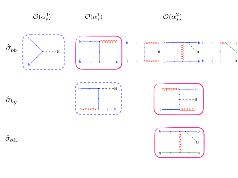
As already mentioned, all $B_{ij}^{(0),(p)}$ terms in Eq. (12) may be equivalently viewed as contributions to the 5FS computation, as schematically summarized in Fig. 1 (for real emission terms). In fact, because no simple closed-form expression of the massive coefficients $B_{ij}^{(p)}$ is available, it turns out to be more convenient to extract the $B_{ij}^{(0),(p)}$ from the 5FS result, as it was done in Ref. [6]. This is simply done by expressing the 5FS $b$ PDF in terms of the 4FS light quark and gluon PDFs up to ${\cal O}(\alpha_{s})$ using the matching coefficients from Ref. [9] (see also Appendix C of Ref. [4]), and then re-expressing the result in terms of the 5FS quark and gluon PDF, and 5FS $\alpha_{s}$.

The result has the structure

$$f_{b}^{(5)}(x,Q^{2})=\alpha^{(5)}_{s}(Q^{2})\int_{x}^{1}\frac{dz}{z} \left\{\mathcal{A}_{gb}^{(1)}\left(z,L\right)f^{(5)}_{g}\left(\frac{x}{z},Q^{2}\right)\vphantom{\frac{\alpha_{s}^{(5)}(Q^{2})}{2\pi}}\right.$$

$$+ \left.\alpha_{s}(Q^{2})\left[\mathcal{A}_{gb}^{(2)}\left(z,L\right)f^{(5)}_{g}\left(\frac{x}{z},Q^{2}\right)+\mathcal{A}_{\Sigma b}^{(2)}\left(z,L\right)f^{(5)}_{\Sigma}\left(\frac{x}{z},Q^{2}\right)\right]\right\}.$$ (16)

where $f^{(5)}_{b}$, $f^{(5)}_{\Sigma}$ and $f^{(5)}_{g}$ are respectively the 5FS $b$ quark, singlet, and gluon PDFs, and

$$\mathcal{A}_{gb}^{(1)} =a_{gb}^{(1,1)}(z)\,L,$$

$$\mathcal{A}_{gb}^{(2)} =a_{gb}^{(2,2)}(z)L^{2}+a_{gb}^{(2,1)}(z)L+a_{gb}^{(2,0)}(z),$$ (17)

$$\mathcal{A}_{\Sigma b}^{(2)} =a_{\Sigma b}^{(2,2)}(z)L^{2}+a_{\Sigma b}^{(2,1)}(z)L+a_{\Sigma b}^{(2,0)}(z)$$

Note that, as well known, to ${\cal O}(\alpha_{s}^{2})$ the expression of the 5FS $f^{(5)}_{b}$ in terms of the light quarks and gluon receives constant (i.e. non-logarithmic) contributions $a_{gb}^{(2,0)}(z)$ and $a_{\Sigma b}^{(2,0)}(z)$, and thus it is discontinuous at threshold $Q^{2}=m_{b}^{2}$ in the massless scheme, as a consequence of it being continuous in the fully massive calculation. The explicit expressions of the coefficients Eq. (S0.Ex2) are given in Appendix A for completeness.

We can now collect all contributions to $\sigma^{(4),(0)}$. The ${\cal O}(\alpha_{s}^{2})$ terms, already given in Ref. [6], are

$$B_{gg}^{(0)(2)}(y,L) =y\int_{y}^{1}\frac{dz}{z}\left[2\mathcal{A}_{gb}^{(1)}\left(z,L\right)\mathcal{A}_{gb}^{(1)}\left(\frac{y}{z},L\right)+4\mathcal{A}_{gb}^{(1)}\left(\frac{y}{z},L\right)\frac{1}{z}\hat{\sigma}_{gb}^{(1)}(z)\right]+\hat{\sigma}_{gg}^{(2)}(y),$$ (18)

$$B_{q\bar{q}}^{(0)(2)}(y,L) =\hat{\sigma}_{q\bar{q}}^{(2)}(y);$$ (19)

while the new contributions to ${\cal O}(\alpha_{s}^{3})$ are

$$B_{gg}^{(0)(3)}(y,L) =y\int_{y}^{1}\frac{dz}{z}\left[4\mathcal{A}_{gb}^{(2)}\left(z,L\right)\mathcal{A}_{gb}^{(1)}\left(\frac{y}{z},L\right)\right.$$

$$+2\mathcal{A}_{gb}^{(2)}\left(\frac{y}{z},L\right)\int_{z}^{1}\frac{dw}{w}\mathcal{A}_{gb}^{(1)}\left(\frac{z}{w},L\right)\frac{1}{w}\hat{\sigma}_{b\bar{b}}^{(1)}(w)$$ (20)

$$\left.\phantom{asdfdy\int_{y}^{1}\frac{dz}{z}4\mathcal{A}_{gb}^{(2)}\left(z,L\right)}+4\mathcal{A}_{gb}^{(2)}\left(\frac{y}{z},L\right)\frac{1}{z}\hat{\sigma}_{gb}^{(1)}(z)+4\mathcal{A}_{gb}^{(1)}\left(\frac{y}{z},L\right)\frac{1}{z}\hat{\sigma}_{gb}^{(2)}(z)\right],$$

$$B_{gq}^{(0)(3)}(y,L) =y\int_{y}^{1}\frac{dz}{z}\left[2\mathcal{A}_{\Sigma b}^{(2)}\left(z,L\right)\mathcal{A}_{gb}^{(1)}\left(\frac{y}{z},L\right)+2\mathcal{A}_{\Sigma b}^{(2)}\left(\frac{y}{z},L\right)\frac{1}{z}\hat{\sigma}_{gb}^{(1)}(z)\right.$$

$$\left.\phantom{asdfdy\int_{y}^{1}\frac{dz}{z}4\mathcal{A}_{gb}^{(2)}\left(z,L\right)\mathcal{A}_{gb}^{(1)}\left(\frac{y}{z},L\right)\mathcal{A}_{gb}^{(1)}\left(\frac{y}{z},L\right)}+2\mathcal{A}_{gb}^{(1)}\left(\frac{y}{z},L\right)\frac{1}{z}\hat{\sigma}_{qb}^{(2)}(z)\right],$$ (21)

which completes our result. Note that in Eq. (S0.Ex4) $\hat{\sigma}_{ij}^{(p)}(x)$ denotes the partonic cross-section in the 5FS, as indicated by the fact that it only depends on the momentum fraction and does not have any dependence on $m_{b}$ (unlike the 4FS partonic cross sections $\hat{\sigma}_{ij}^{(p)}\left(x,\frac{Q^{2}}{m_{b}^{2}}\right)$ of Eq. (5)).

Figure 2: Comparison of the FONLL matched result and its 4FS and 5FS components, Eq. (1). Results are shown as a function of the renormalization scale, with the factorization scale fixed at a high value $\mu_{F}=m_{H}$ (top) or a low value $\mu_{F}=\frac{(m_{H}+2m_{b})}{4}$ (bottom).

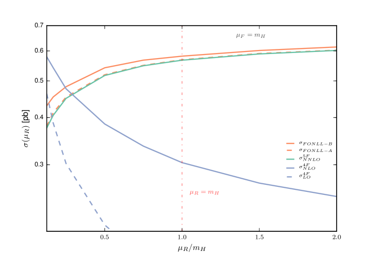
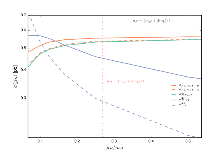
We have implemented our final FONLL-B expression by combining, according to Eq. (1) 4FS predictions up to NLO obtained using MG5_aMC@NLO [10, 11], 5FS computations up to NNLL obtained using the bbh@nnlo code [1], and our own implementation of the subtraction term Eq. (12).

Figure 3: Same as Fig. 2, but now with the factorization scale varied with the renormalization scale kept fixed at a high value $\mu_{R}=m_{H}$ (top) or a low value $\mu_{R}=\frac{(m_{H}+2m_{b})}{4}$ (bottom) .

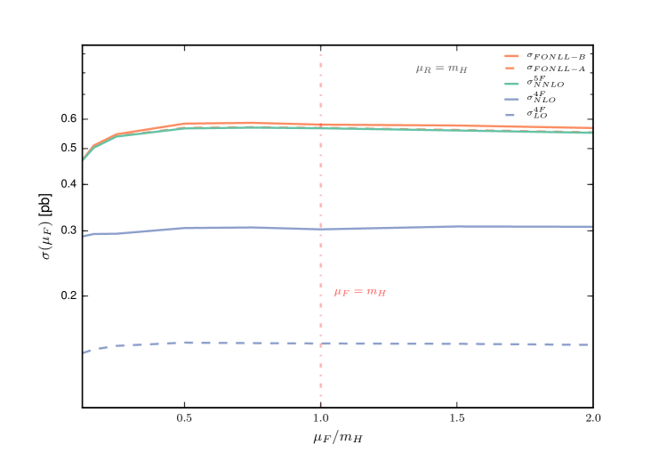
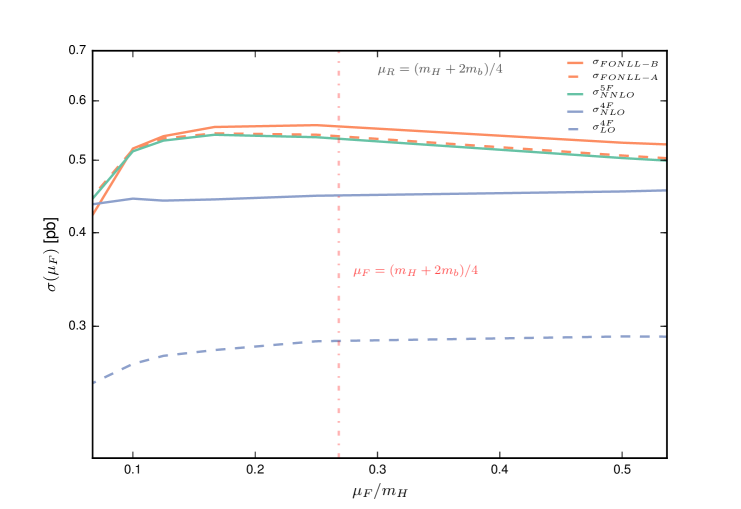
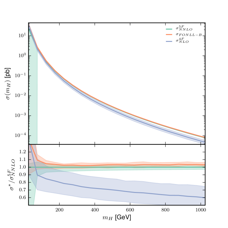
In Figs. 2-4 we compare the 4FS, 5FS and matched FONLL results. Specifically, in Figs. 2-3 we show for the physical Higgs mass value $m_{H}=125$ GeV, varying the renormalization and factorization scale both the LO and NLO 4FS predictions, and the FONLL-A and FONLL-B matched results in which they are respectively combined with the NNLL 5FS result, also shown. In Fig. 4 we show the most accurate results obtained in the 4FS (NLO), 5FS (NNLO) and matched (FONLL-B) schemes, as a function of the Higgs mass, with $\mu_{R}=\mu_{F}=\frac{m_{H}+4m_{B}}{4}$, and the uncertainty band obtained by taking the envelope of the variations of the renormalization and factorization scales by a factor two about the central value with the two outer points $\mu_{R}=4\mu_{F}$ and $\mu_{F}=4\mu_{r}$ omitted. Note that for the lowest (unphysical) Higgs mass values this uncertainty blows up because the lower edge of the scale variation range extends in the nonperturbative region.

The 4FS results shown are those which enter the FONLL combination, namely, the form Eq. (2) of the 4FS result is used, in which this is expressed in terms of 5FS PDFs and $\alpha_{s}$. All results are computed using a PDF set presented and discussed in Ref. [12]. This PDF set is based on the PDF4LHC15 combined sets [13, 14, 15, 16, 17, 18, 19], with which it is taken to coincide below the $b$ mass, but from which it is then evolved up in the $5FS$ from $Q=m_{b}$, with the results below and above threshold matched exactly as in Eq. (S0.Ex1). This is not quite the same as the original PDF4LHC15 combination, which is obtained by combining sets which adopt different values of $m_{b}$, and also incorporate subleading differences in the way the 4FS and 5FS are matched at threshold: it thus has the advantage of being fully consistent. We use pole-mass expressions and take a $b$ pole-mass value $m_{b}=4.58$ GeV; the strong coupling is $\alpha_{s}(m_{Z})=0.118$.

Figure 4: The cross-section using the most accurate results in the 4FS (NLO), 5FS (NNLO) and matched (FONLL-B) schemes, as a function of the Higgs mass, with $\mu_{r}=\mu_{F}=\frac{(m_{H}+2m_{b})}{4}$. The bottom panel shows the result as a ratio to the 5FS computation. The uncertainty band is obtained by standard seven-point scale variation (see text).

From Fig. 2 we see that the strong renormalization scale dependence of the LO 4FS result is reduced at NLO, and also, that at NLO the big gap between the 4FS and 5FS results gets compensated for by the inclusion of higher order terms in the 4FS. This, together with the fact that the 5FS shows very little scale dependence, and that differences are significantly smaller for smaller values of $\mu_{F}$, strongly suggests that the bulk of the difference between the 4FS and the 5FS is due to large logs of $\mu_{F}^{2}/m_{b}^{2}$ which are resummed into the PDF in the latter case. This is in agreement with the conclusion of Ref. [5], in which it was shown that resummation increases the cross section in most cases by up to 30% at the LHC, leading to a better precision. On the other hand, the 4FS predictions at NLO also displays a consistent perturbative behaviour only when evaluated at a suitably low scale.

The massive corrections which the 4FS result contains turn out to be much smaller, though not entirely negligible. Indeed, whereas the FONLL-A result essentially coincides with the 5FS, the FONLL-B, which only differs from it because of the inclusion of massive terms at one extra perturbative order, departs somewhat from it. The factorization scheme dependence shown in Fig. 3 is very mild in all schemes when $\mu_{R}$ is high, but for low $\mu_{R}$, where the perturbative expansion of the 4FS result is more reliable, both the 5FS and the FONLL-A results show a contained scale dependence, comparable in size to the mass effects, which is reduced in the FONLL-B result.

These results suggest that the main difference between the FONLL-A and the FONLL-B schemes is the inclusion of a higher order contribution from the 4FS computation which reduces the the scale dependence of the FONLL-A result; because the latter is essentially the same as that of the 5FS computation this contribution is likely to be dominated by a constant, i.e., mass-independent term. This conclusion is supported by Fig. 4, in which results are shown as a function of the Higgs mass: the difference between the FONLL-B and 5FS results decreases slightly as the mass grows until $m_{H}\sim 200$ GeV, but then it remains constant up to the highest values of the Higgs mass.

We conclude that the FONLL-B result is the most reliable, and a low choice of renormalization and factorization scheme seems to lead to a more reliable perturbative expansion, but all in all mass corrections are very moderate, so the usage of the 5FS result at all scales would be adequate in most cases. This rather disfavours phenomenological combinations such as the so-called Santander matching [20] in which the 4FS and 5FS results are combined through an interpolation that gives each of them comparable weight. The difference between the FONLL-B and 5FS is almost entirely due to a constant $O(\alpha_{s}^{3})$ mass-independent contribution which appears in the 4FS at NLO but would only enter the 5FS at N³LO; the FONLL-B computation, which includes it, is accordingly more accurate, even for very high vales of the Higgs mass.

Matched results for this process were recently obtained in Refs. [21, 12] using an effective field theory approach, and a somewhat different counting of perturbative orders. A benchmarking of our results with those of these references has been performed in the context of the Higgs cross section working group, and it will be presented there [22]. In that benchmarking the matched calculations are found to agree to within better than $5\%$ when results at the same perturbative orders are included, with the residual difference due to a somewhat different choice of factorization and renormalization scales in the two computations which are being compared.

In summary, we have presented a matched computation of Higgs production in association with bottom quarks including known results to the highest available accuracy, namely, NLO in a four-flavor scheme in which $b$ quark mass effects are fully accounted for, and NNLL in a five-flavor scheme in which the $b$ quark is treated as a massless parton with collinear logs resummed to all orders. We find that mass corrections are very small while collinear logs are substantial, so that in practice the fully matched result is very close to the 5FS one. The fully matched result receives a small correction from mass effects and it is very stable upon renormalization and factorization scheme variation, suggesting that it is adequate for precision phenomenology at the LHC.

A public implementation of our NNLL+NLO FONLL-B matched computation will be made available from:

http://bbhfonll.hepforge.org/

Appendix A Appendix A

We give for completeness the expressions of the coefficients Eq. (S0.Ex2). These were computed in Ref. [9]. There are a few differences compared to what is presented there. Firstly we separate contributions from $b$ and $\bar{b}$. Secondly our expansion is done in powers of $\alpha_{s}$ rather than in powers of $\frac{\alpha_{s}}{4\pi}$. Lastly we have re-expressed the gluon and singlet PDFs in the 4FS in terms of those computed in the 5FS.

$$\mathcal{A}^{(2)}_{\Sigma b}(z,L) =\frac{1}{32\pi^{2}}C_{F}T_{f}\Biggl{\{}\Biggl{[}-8(1+z)\ln z-\frac{16}{3z}-4+4z+\frac{16}{3}z^{2}\Biggr{]}L^{2}$$

$$-\Biggl{[}8(1+z)\ln^{2}z-\Biggl{(}8+40z+\frac{64}{3}z^{2}\Biggr{)}\ln z-\frac{160}{9z}+16-48z+\frac{448}{9}z^{2}\Biggr{]}L$$

$$+(1+z)\Biggl{[}32{\rm S}_{1,2}(1-z)+16\ln z{\rm Li}_{2}(1-z)-16\zeta(2)\ln z-\frac{4}{3}\ln^{3}z\Biggr{]}$$

$$+\Biggl{(}\frac{32}{3z}+8-8z-\frac{32}{3}z^{2}\Biggr{)}{\rm Li}_{2}(1-z)+\Biggl{(}-\frac{32}{3z}-8+8z+\frac{32}{3}z^{2}\Biggr{)}\zeta(2)$$

$$+\Biggl{(}2+10z+\frac{16}{3}z^{2}\Biggr{)}\ln^{2}z-\Biggl{(}\frac{56}{3}+\frac{88}{3}z+\frac{448}{9}z^{2}\Biggr{)}\ln z-\frac{448}{27z}-\frac{4}{3}-\frac{124}{3}z+\frac{1600}{27}z^{2}\Biggr{\}}\,,$$ (A.1)

$$\mathcal{A}_{gb}^{(1)}(z,L) =\frac{T_{f}}{2\pi}\Biggl{[}(z^{2}+(1-z)^{2})L\Biggr{]}\,,$$ (A.2)

and

$$\!\!\!\!\!\!\!\!\!\!\!\!\!\!\!\!\!\!\mathcal{A}_{bg}^{(2)}(z,L) =\frac{1}{32\pi^{2}}\Biggl{\{}\Biggl{\{}C_{F}T_{f}[(8-16z+16z^{2})\ln(1-z)-(4-8z+16z^{2})\ln z-(2-8z)]$$

$$+C_{A}T_{f}\Biggl{[}-(8-16z+16z^{2})\ln(1-z)-(8+32z)\ln z-\frac{16}{3z}-4-32z+\frac{124}{3}z^{2}\Biggr{]}\Biggr{\}}L^{2}$$

$$-\Biggl{\{}C_{F}T_{f}\Biggl{[}(8-16z+16z^{2})[2\ln z\ln(1-z)-\ln^{2}(1-z)+2\zeta(2)]$$

$$-(4-8z+16z^{2})\ln^{2}z-32z(1-z)\ln(1-z)-(12-16z+32z^{2})\ln z-56+116z-80z^{2}\Biggr{]}$$

$$+C_{A}T_{f}\Biggl{[}(16+32z+32z^{2})[{\rm Li}_{2}(-z)+\ln z\ln(1+z)]+(8-16z+16z^{2})\ln^{2}(1-z)$$

$$+(8+16z)\ln^{2}z+32z\zeta(2)+32z(1-z)\ln(1-z)-\Biggl{(}8+64z+\frac{352}{3}z^{2}\Biggr{)}\ln z$$

$$-\frac{160}{9z}+16-200z+\frac{1744}{9}z^{2}\Biggr{]}\Biggl{\}}L$$

$$+C_{F}T_{f}\Biggl{\{}(1-2z+2z^{2})[8\zeta(3)+\frac{4}{3}\ln^{3}(1-z)-8\ln(1-z){\rm Li}_{2}(1-z)+8\zeta(2)\ln z$$

$$-4\ln z\ln^{2}(1-z)+\frac{2}{3}\ln^{3}z-8\ln z{\rm Li}_{2}(1-z)+8{\rm Li}_{3}(1-z)-24{\rm S}_{1,2}(1-z)]$$

$$+z^{2}\Biggl{[}-16\zeta(2)\ln z+\frac{4}{3}\ln^{3}z+16\ln z{\rm Li}_{2}(1-z)+32{\rm S}_{1,2}(1-z)\Biggr{]}$$

$$-(4+96z-64z^{2}){\rm Li}_{2}(1-z)-(4-48z+40z^{2})\zeta(2)$$

$$-(8+48z-24z^{2})\ln z\ln(1-z)+(4+8z-12z^{2})\ln^{2}(1-z)$$

$$-(1+12z-20z^{2})\ln^{2}z-(52z-48z^{2})\ln(1-z)$$

$$-(16+18z+48z^{2})\ln z+26-82z+80z^{2}\Biggr{\}}$$

$$+C_{A}T_{f}\Biggl{\{}(1-2z+2z^{2})[-\frac{4}{3}\ln^{3}(1-z)$$

$$+8\ln(1-z){\rm Li}_{2}(1-z)-8{\rm Li}_{3}(1-z)]+(1+2z+2z^{2})$$

$$\times[-8\zeta(2)\ln(1+z)-16\ln(1+z){\rm Li}_{2}(-z)-8\ln z\ln^{2}(1+z)$$

$$+4\ln^{2}z\ln(1+z)+8\ln z{\rm Li}_{2}(-z)-8{\rm Li}_{3}(-z)-16{\rm S}_{1,2}(-z)]$$

$$+(16+64z)[2{\rm S}_{1,2}(1-z)+\ln z{\rm Li}_{2}(1-z)]-\Biggl{(}\frac{4}{3}+\frac{8}{3}z\Biggr{)}\ln^{3}z$$

$$+(8-32z+16z^{2})\zeta(3)-(16+64z)\zeta(2)\ln z+(16+16z^{2})$$

$$\times[{\rm Li}_{2}(-z)+\ln z\ln(1+z)]+\Biggl{(}\frac{32}{3z}+12+64z-\frac{272}{3}z^{2}\Biggr{)}{\rm Li}_{2}(1-z)$$

$$-\Biggl{(}12+48z-\frac{260}{3}z^{2}+\frac{32}{3z}\Biggr{)}\zeta(2)-4z^{2}\ln z\ln(1-z)$$

$$-(2+8z-10z^{2})\ln^{2}(1-z)+\Biggl{(}2+8z+\frac{46}{3}z^{2}\Biggr{)}\ln^{2}z$$

$$+(4+16z-16z^{2})\ln(1-z)-\Biggl{(}\frac{56}{3}+\frac{172}{3}z+\frac{1600}{9}z^{2}\Biggr{)}\ln z$$

$$-\frac{448}{27z}-\frac{4}{3}-\frac{628}{3}z+\frac{6352}{27}z^{2}\Biggr{\}}\Biggr{\}}\,.$$ (A.3)

References

- [1] R. V. Harlander and W. B. Kilgore, Higgs boson production in bottom quark fusion at next-to-next-to leading order, Phys. Rev. D68 (2003) 013001, [hep-ph/0304035].
- [2] S. Dittmaier, M. Kramer, 1, and M. Spira, Higgs radiation off bottom quarks at the Tevatron and the CERN LHC, Phys. Rev. D70 (2004) 074010, [hep-ph/0309204].
- [3] S. Dawson, C. B. Jackson, L. Reina, and D. Wackeroth, Exclusive Higgs boson production with bottom quarks at hadron colliders, Phys. Rev. D69 (2004) 074027, [hep-ph/0311067].
- [4] F. Maltoni, G. Ridolfi, and M. Ubiali, b-initiated processes at the LHC: a reappraisal, JHEP 07 (2012) 022, [arXiv:1203.6393]. [Erratum: JHEP04,095(2013)].
- [5] M. Lim, F. Maltoni, G. Ridolfi, and M. Ubiali, Anatomy of double heavy-quark initiated processes, arXiv:1605.09411.
- [6] S. Forte, D. Napoletano, and M. Ubiali, Higgs production in bottom-quark fusion in a matched scheme, Phys. Lett. B751 (2015) 331–337, [arXiv:1508.01529].
- [7] M. Cacciari, M. Greco, and P. Nason, The P(T) spectrum in heavy flavor hadroproduction, JHEP 05 (1998) 007, [hep-ph/9803400].
- [8] S. Forte, E. Laenen, P. Nason, and J. Rojo, Heavy quarks in deep-inelastic scattering, Nucl. Phys. B834 (2010) 116–162, [arXiv:1001.2312].
- [9] M. Buza, Y. Matiounine, J. Smith, and W. L. van Neerven, Charm electroproduction viewed in the variable flavor number scheme versus fixed order perturbation theory, Eur. Phys. J. C1 (1998) 301–320, [hep-ph/9612398].
- [10] J. Alwall, R. Frederix, S. Frixione, V. Hirschi, F. Maltoni, O. Mattelaer, H. S. Shao, T. Stelzer, P. Torrielli, and M. Zaro, The automated computation of tree-level and next-to-leading order differential cross sections, and their matching to parton shower simulations, JHEP 07 (2014) 079, [arXiv:1405.0301].
- [11] M. Wiesemann, R. Frederix, S. Frixione, V. Hirschi, F. Maltoni, and P. Torrielli, Higgs production in association with bottom quarks, JHEP 02 (2015) 132, [arXiv:1409.5301].
- [12] M. Bonvini, A. S. Papanastasiou, and F. J. Tackmann, Matched predictions for the cross section at the 13 TeV LHC, arXiv:1605.01733.
- [13] J. Butterworth et al., PDF4LHC recommendations for LHC Run II, J. Phys. G43 (2016) 023001, [arXiv:1510.03865].
- [14] NNPDF Collaboration, R. D. Ball et al., Parton distributions for the LHC Run II, JHEP 04 (2015) 040, [arXiv:1410.8849].
- [15] L. A. Harland-Lang, A. D. Martin, P. Motylinski, and R. S. Thorne, Parton distributions in the LHC era: MMHT 2014 PDFs, Eur. Phys. J. C75 (2015), no. 5 204, [arXiv:1412.3989].
- [16] S. Dulat, T.-J. Hou, J. Gao, M. Guzzi, J. Huston, P. Nadolsky, J. Pumplin, C. Schmidt, D. Stump, and C. P. Yuan, New parton distribution functions from a global analysis of quantum chromodynamics, Phys. Rev. D93 (2016), no. 3 033006, [arXiv:1506.07443].
- [17] S. Carrazza, S. Forte, Z. Kassabov, J. I. Latorre, and J. Rojo, An Unbiased Hessian Representation for Monte Carlo PDFs, Eur. Phys. J. C75 (2015), no. 8 369, [arXiv:1505.06736].
- [18] J. Gao and P. Nadolsky, A meta-analysis of parton distribution functions, JHEP 07 (2014) 035, [arXiv:1401.0013].
- [19] G. Watt and R. S. Thorne, Study of Monte Carlo approach to experimental uncertainty propagation with MSTW 2008 PDFs, JHEP 08 (2012) 052, [arXiv:1205.4024].
- [20] R. Harlander, M. Kramer, and M. Schumacher, Bottom-quark associated Higgs-boson production: reconciling the four- and five-flavour scheme approach, arXiv:1112.3478.
- [21] M. Bonvini, A. S. Papanastasiou, and F. J. Tackmann, Resummation and matching of b-quark mass effects in production, JHEP 11 (2015) 196, [arXiv:1508.03288].
- [22] LHC Higgs Cross Section Working Group Collaboration, C. Anastasiou et al., Handbook of LHC Higgs Cross Sections: 4. Deciphering the nature of the Higgs sector, in preparation.