An Application of ParaExp to Electromagnetic Wave Problems

Abstract

Recently, ParaExp was proposed for the time integration of hyperbolic problems. It splits the time interval of interest into sub-intervals and computes the solution on each sub-interval in parallel. The overall solution is decomposed into a particular solution defined on each sub-interval with zero initial conditions and a homogeneous solution propagated by the matrix exponential applied to the initial conditions. The efficiency of the method results from fast approximations of this matrix exponential using tools from linear algebra. This paper deals with the application of ParaExp to electromagnetic wave problems in time-domain. Numerical tests are carried out for an electric circuit and an electromagnetic wave problem discretized by the Finite Integration Technique.

I Introduction

The simulation of high-frequency electromagnetic problems is often carried out in frequency domain. This choice is motivated by the linearity of the underlying governing equations and an implicit assumption that the source signal can be decomposed in the Fourier basis.

However, the solution of problems in frequency domain may require the resolution of very large linear systems of equations and this becomes particularly inconvenient for broadband simulations involving multi-frequency sources such as Gaussian or pulsed signals. The coupling with nonlinear time-dependent systems and the computation of transients are other cases where time-domain simulations outperform frequency-domain simulations. On the other hand, the numerical complexity resulting from time-domain simulations may also become prohibitively expensive; time-domain parallelization is a promising solution alternative to domain decomposition in space.

The development and application of parallel-in-time methods dates back to more than 50 years [1]. These methods can be direct [2, 3] or iterative [4, 5]. They can also be well suited for small scale parallelization [6, 7] or large parallelization [3, 5]. Recently, the Parareal method gained interest [4, 8]. In its initial version, Parareal was developed for large scale parallelization of parabolic partial differential equations (PDEs). It involves the splitting of the time interval and the resolution of the governing ordinary differential equation (ODE) in parallel on each sub-intervals using a fine propagator which can be any classical time-stepper with a fine time grid. A coarse propagator distributes the initial conditions for each sub-interval during the Parareal iterations. It is typically obtained by a time stepper with a coarse grid on the entire time interval. Parareal iterates the resolution of both the coarse and the fine problems until convergence.

Most parallel-in-time methods fail for hyperbolic problems. In the case of Parareal, analysis has shown that it may lead to the beating phenomenon depending on the structure of the system matrix obtained after space discretization [9]. It may even become unstable if the eigenvalues of the matrix are pure imaginary which is the case in the presence of undamped electromagnetic waves.

In this paper we apply the ParaExp method [3] for the parallelization of time-domain resolutions of hyperbolic equations that govern the electromagnetic wave problems. The method splits the time interval into sub-intervals and solves smaller problems on each sub-interval as visualized in Figure 1. Using the theory of linear ordinary differential equations, the total solution for each sub-interval is decomposed into particular solution with zero initial conditions and homogeneous solutions with initial conditions from previous intervals.

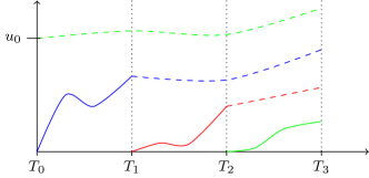
Figure 1: Schematic view of the decomposition of time and solution. Vertical dotted lines denote the sub-intervals, solid lines represent the solution of the inhomogeneous sub-problems and dashed lines represent the solution of the homogeneous sub-problems. Colors indicate the employed processors, cf. [3]

The paper is organized as follows: in Section II we introduce Maxwell’s equations and derive the governing system of ODEs for the wave equation obtained by the Finite Integration Technique (FIT) or Finite Element Method (FEM). This system is then used in Section III for the presentation of the ParaExp method following the lines of [3]. The mathematical framework is briefly sketched and the details of the algorithm are discussed. Section IV deals with numerical examples. We consider two applications: a simple RLC circuit and an electromagnetic wave problem in an open wave guide. The accuracy of the method and the accuracy of the method in terms of the electromagnetic energy are investigated.

II Space and Time Discretization of Maxwell’s equations

In an open, bounded domain $\Omega\subset\mathbb{R}^{3}$ and $t\in\mathcal{I}=(t_{0},t_{\mathrm{end}}]\subset\mathbb{R}$, the evolution of electromagnetic fields is governed by Maxwell’s Equations on $\Omega\times\mathcal{I}$, see e.g. [10]:

$$\text{\text{curl}}{}\,{\mbox{\boldmath$h$}}=\mbox{\boldmath$j$}+\partial_{t}\mbox{\boldmath$d$},\,\,\text{\text{curl}}{}\,{\mbox{\boldmath$e$}}=-\partial_{t}\mbox{\boldmath$b$},\,\,\text{\text{div}}{}\,{\mbox{\boldmath$d$}}=\rho,\,\,\text{\text{div}}{}\,{\mbox{\boldmath$b$}}=0.$$ (1)

In presence of linear materials, these equations are completed by constitutive laws [10]:

$$\mbox{\boldmath$j$}=\sigma\mbox{\boldmath$e$}+\mbox{\boldmath$j$}_{s},\quad\mbox{\boldmath$d$}=\varepsilon\mbox{\boldmath$e$},\quad\mbox{\boldmath$b$}=\mu\mbox{\boldmath$h$}.$$ (2)

In these equations, $h$ is the magnetic field [A/m], $b$ the magnetic flux density [T], $e$ the electric field [V/m], $d$ the electric flux density [C/m²], $j$, $\mbox{\boldmath$j$}_{\rm d}=\partial_{t}\mbox{\boldmath$d$}$ and $\mbox{\boldmath$j$}_{s}$ are the Ohmic, displacement and electric source current densities [A/m²], $\rho$ is the electric charge density [C/m³]. The material properties $\sigma,\varepsilon$ and $\mu$ are the electric conductivity, the electric permittivity and the magnetic permeability, respectively. In this paper, we consider electromagnetic wave propagation in non-conducting media and which are free of charge, i.e., $\sigma\equiv 0$ and $\rho\equiv 0$. However, that the algorithms can be easily applied to the general case.

The space discretization of Maxwell’s equations (1)-(2) using the Finite Integration Technique (FIT) [11, 12] leads to the following initial value problem (IVP)

$${\bf M}\mathrm{d_{t}}\mathbf{u}+{\bf K}\mathbf{u}=\bar{\mathbf{g}}(t)\quad\forall t\in\mathcal{I},\quad\mathbf{u}(t_{0})=\mathbf{u}_{0}.$$ (3)

with $\mathbf{u}^{\top}=[\vbox{\halign{#\cr$\scriptscriptstyle\mathord{\frown}\mkern-0.2mu\cleaders\hbox{$\mkern-2.0mu\smash{-}\mkern-2.0mu$}\hfill\mkern-0.2mu$\crcr\kern-0.2pt\nointerlineskip\cr$\hfil\displaystyle{\rm\bf h}\hfil$\crcr}}^{\top},\vbox{\halign{#\cr$\scriptscriptstyle\mathord{\frown}\mkern-0.2mu\cleaders\hbox{$\mkern-2.0mu\smash{-}\mkern-2.0mu$}\hfill\mkern-0.2mu$\crcr\kern-0.2pt\nointerlineskip\cr$\hfil\displaystyle{\rm\bf e}\hfil$\crcr}}^{\top}]$, $\bar{\mathbf{g}}(t)$ which is an excitation and the matrices ${\bf M}$ and ${\bf K}$ given by:

$${\bf M}:=\begin{bmatrix}{\bf M}_{\mu}^{\mathrm{FIT}}&\boldsymbol{0}\\ \boldsymbol{0}&{\bf M}_{\varepsilon}^{\mathrm{FIT}}\end{bmatrix}\,,\,{\bf K}:=\begin{bmatrix}\boldsymbol{0}&{\bf C}\\ -\widetilde{{\bf C}}&\boldsymbol{0}\end{bmatrix}.$$ (4)

${\bf M}_{\varepsilon}^{\mathrm{FIT}}$ and ${\bf M}_{\mu}^{\mathrm{FIT}}$ are diagonal material matrices and ${\bf C}$ and $\widetilde{{\bf C}}$ are the discrete curl operators defined on the primal and dual grids, respectively; ${\bf M}$ is invertible, thus (3) can be written as:

$$\mathrm{d_{t}}\mathbf{u}={\bf A}\mathbf{u}+{\mathbf{g}}(t)\quad\forall t\in\mathcal{I},\quad\mathbf{u}(t_{0})=\mathbf{u}_{0}$$ (5)

with ${\bf A}:=-{\bf M}^{-1}{\bf K}$ and ${\mathbf{g}}(t):={\bf M}^{-1}\bar{\mathbf{g}}(t)$. Typically this system is time-integrated using the Leapfrog scheme.

Similarly, the use of the FE method applied to the $e$-formulation leads to the following weak form: find $e$ in an appropriate function space [13] such that

$$\left(\varepsilon\partial_{tt}\mbox{\boldmath$e$},\mbox{\boldmath$e$}^{{}^{\prime}}\right)_{\Omega}+\left(\mu^{-1}\text{\text{curl}}{}\,{\mbox{\boldmath$e$}},\text{\text{curl}}{}\,{\mbox{\boldmath$e$}^{{}^{\prime}}}\right)_{\Omega}\\ =-\left(\partial_{t}\mbox{\boldmath$j$}_{s},\mbox{\boldmath$e$}^{{}^{\prime}}\right)_{\Omega_{s}}+\Big{<}(\mu^{-1}\text{\text{curl}}{}\,{\mbox{\boldmath$e$}}\times\mbox{\boldmath$n$}),\mbox{\boldmath$e$}^{{}^{\prime}}\Big{>}_{\Gamma}$$ (6)

holds for all test functions $\mbox{\boldmath$e$}^{{}^{\prime}}$ in a space of test functions. In (6), $\Gamma=\partial\Omega$ is the boundary of $\Omega$. Space discretization of (6) using the Galerkin approach leads to the system of ODEs:

$${\bf M}_{\varepsilon}^{\mathrm{FE}}\mathrm{d_{tt}}\mbox{\boldmath$e$}+{\bf K}_{\mu^{-1}}^{\mathrm{FE}}\mbox{\boldmath$e$}=\bar{\mathbf{g}}^{\mathrm{FE}}(t)\quad\forall t\in\mathcal{I},$$ (7)

$$\mbox{\boldmath$e$}(t_{0})=\mbox{\boldmath$e$}_{0},\quad\mathrm{d}_{t}\mbox{\boldmath$e$}(t_{0})=\mbox{\boldmath$e$}_{1}.$$

where the matrices ${\bf M}_{\varepsilon}^{\mathrm{FE}}$ and ${\bf K}_{\mu^{-1}}^{\mathrm{FE}}$ in (7) are FEM material matrices obtained from the discretization of the bilinear forms in (6) and $\bar{\mathbf{g}}^{\mathrm{FE}}(t)$ is the source term. Equation (7) can be recast in a first order system similar to (3).

III The ParaExp Algorithm

In this section we develop based on [3] the ideas of the ParaExp method for the system of ODEs in the form (5)

$$\mathrm{d_{t}}\mathbf{u}=\mathbf{{\bf A}}\mathbf{u}+\mathbf{g}(t)\quad\forall t\in\mathcal{I},\quad\mathbf{u}(t_{0})=\mathbf{u}_{0}.$$ (8)

Applying the method of variation of constants to equation (8) leads to the solution

$$\mathbf{u}(t)=\exp{(t{\bf A}})\mathbf{u}_{0}+\int_{0}^{t}\exp{((t-\tau){\bf A})}\mathbf{g}(\tau)\mathrm{d}\tau$$ (9)

where $\exp{(t{\bf A}})\mathbf{u}_{0}$ is the homogeneous solution due to initial conditions and the convolution product is the particular solution resulting from the presence of the source term $\mathbf{g}(t)$. The last term of (9) is more difficult to compute than the first one. However, thanks to the linearity of equation (8) and the superposition principle, $\mathbf{u}(t)$ can be written as $\mathbf{u}(t)=\mathbf{v}(t)+\mathbf{w}(t)$ where the particular solution $\mathbf{v}(t)$ is governed by

$$\mathrm{d_{t}}\mathbf{v}={\bf A}\mathbf{v}+\mathbf{g}(t)\quad\forall t\in\mathcal{I},\quad\mathbf{v}(t_{0})=\boldsymbol{0}$$ (10)

and the homogeneous solution $\mathbf{w}(t)$ is governed by

$$\mathrm{d_{t}}\mathbf{w}={\bf A}\mathbf{w}+\boldsymbol{0}\quad\forall t\in\mathcal{I},\quad\mathbf{w}(t_{0})=\mathbf{u}_{0}.$$ (11)

The ParaExp method takes advantage of this decomposition. The time interval (0, T] is partitioned into sub-intervals $\mathcal{I}_{j}=(T_{\mathrm{j-1}},T_{\mathrm{j}}]$ with $j=1,2,...,p$, $t_{0}=T_{0}<T_{1}<T_{2}<...<T_{p}=t_{\mathrm{end}}$ and $p$ the number of CPUs. The following solutions are then computed on each CPU:

1. a particular solution $\mathbf{v}_{j}(t)$ governed by:

   $$\mathrm{d_{t}}\mathbf{v}_{j}={\bf A}\mathbf{v}_{j}+\mathbf{g}(t) \forall t\in\mathcal{I}_{j},$$ (12)

   $$\mathbf{v}_{j}(T_{j-1})=\boldsymbol{0},$$

2. a homogeneous solution $\mathbf{w}_{j}(t)$ governed by:

   $$\mathrm{d_{t}}\mathbf{w}_{j}={\bf A}\mathbf{w}_{j}+\boldsymbol{0} \forall t\in(T_{j-1},T],$$ (13)

   $$\mathbf{w}_{j}(T_{j-1})=\mathbf{v}_{\mathrm{j-1}}(T_{j-1}).$$

Problems (12) can be solved simultaneously in parallel using a time stepping method as no initial conditions need to be provided. Problems (13) are solved on (possibly bigger) time intervals $(T_{j-1},T]$ and they yield exponential solutions $\mathbf{w}_{j}(t)=\exp{(t{\bf A})}\mathbf{v}_{\mathrm{j-1}}(T_{j-1})$ where the initial condition is the final solution $\mathbf{v}_{\mathrm{j-1}}(T_{j-1})$. It is therefore highly recommended to compute $\mathbf{v}_{\mathrm{j-1}}(t)$ and $\mathbf{w}_{\mathrm{j}}(t)$ on the same CPU to avoid communicational costs. Using the superposition principle, the total solution can be expanded as:

$$\mathbf{u}(t)=\mathbf{v}_{j}(t)+\sum_{i=1}^{j}\mathbf{w}_{i}(t)\,\,\textrm{ with }j\textrm{ such that }t\in\mathcal{I}_{j}.$$ (14)

Figure 1 shows the time decomposition of IVP into particular solutions (solid lines) and homogeneous solutions (dashed lines) for a case with 3 CPUs. Steps (a) and (b) of the ParaExp method are described in Algorithm 1.

Input: system matrix $\mathbf{A}$, source term $\mathbf{g}(t)$, initial value $\mathbf{u}_{0}$, time interval $\mathcal{I}$, number of processors $p$

Output: solution $\mathbf{u}(t)$

1 begin

2       set $T_{j}$ (partition $\mathcal{I}$ into intervals $\mathcal{I}_{j}$, $j=0,...,p$),

3       # begin the parallel loop (index $j$)

4       for $(j\leftarrow 1$ to $p)$ do

5             $\mathbf{v}_{j}\leftarrow$ solve $\mathbf{v}_{j}^{\prime}(t)=\mathbf{A}\mathbf{v}_{j}(t)+\mathbf{g}(t)$, $\mathbf{v}_{j}(T_{j-1})=0$, $t\in\mathcal{I}_{j}$ using a time stepper

6             if $j\neq p$ then

7                   $\mathbf{w}_{j+1}\leftarrow\exp(\mathbf{A}(t-T_{j}))\mathbf{v}_{j}(T_{j})$ for all $t\in(T_{j},T_{p}]$

8            else

9                   $\mathbf{w}_{1}\leftarrow\exp(\mathbf{A}(t-T_{0}))\mathbf{u}_{0}$ for all $t\in(T_{0},T_{p}]$

10             end if

11            

12       end for

13      for $(j\leftarrow 1$ to $p)$ do

14             $\mathbf{u}(t)\leftarrow\mathbf{v}_{j}(t)+\sum\limits_{i=1}^{j}\mathbf{w}_{i}(t)$, for all $t\in\mathcal{I}_{j}$

15       end for

16      

17 end

18

Algorithm 1 Pseudocode for the ParaExp Algorithm

A critical point of the method is the computation of the matrix exponential. A straight forward evaluation of the definition is not feasible. Instead, efficient approximations of the action of the matrix exponential should be used, e.g., based on Krylov subspaces [3] or the approximation of the action of the matrix exponential as proposed in [14], where for given integers $s$ and $m$ and for an arbitrary vector $\mathbf{b}$ the relation

$$\exp(t{\bf A})\mathbf{b}=\left(\exp\!\left(s^{-1}t{\bf A}\right)\right)^{s}\mathbf{b}$$

is exploited to build a recurrence

$$\mathbf{u}_{i+1}=\mathbf{r}_{m}\left(s^{-1}t{\bf A}\right)\mathbf{b}_{i},\;\;\;i=0,\dots,s-1,\;\;\;\mathbf{b}_{0}=\mathbf{b},$$

with the truncated Taylor series of order $m$ of the matrix exponential

$$\mathbf{r}_{m}\left(s^{-1}t{\bf A}\right)=\sum\limits_{j=0}^{m}\frac{\left(s^{-1}t{\bf A}\right)^{j}}{j!}.$$

IV Preliminary results

As a proof-of-concept, the ParaExp algorithm is implemented in Octave [15], using the explicit Runge-Kutta method of order 4 (RK4) provided by OdePkg [16] as a time stepper, while no approximation of the matrix exponential was used. The RLC circuit (Fig. 2) with known closed-form solution is constructed as a first test case.

Figure 2: RLC test circuit

The signal of the voltage source is $u_{0}(t)=U_{0}\sin\left(\omega_{0}t\right)$ with $U_{0}=$10\text{\,}\mathrm{V}$$ and $\omega_{0}=2000\pi^{2}$\frac{}{\mathrm{s}}$$. The differential equation of this problem is given by

$$L\mathrm{d_{tt}^{2}}i(t)+R\mathrm{d_{t}}i(t)+C^{-1}i(t)=U_{0}\omega_{0}\cos\left(\omega_{0}t\right)$$ (15)

$$i(0)=0,\qquad\mathrm{d_{t}}i(0)=-{U_{L0}}{L}^{-1}$$ (16)

with $U_{L0}=$12\text{\,}\mathrm{V}$$. Both, RK4 on the whole time interval and ParaExp with three parallel threads, are applied to equation (15). ParaExp executes the RK4 time stepper in each thread and the constant time step size has been chosen in all cases as $\Delta t=$1\text{\times}{10}^{-5}\text{\,}\mathrm{s}$$. The results are compared to the closed-form solution in Fig. 3.

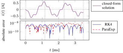
Figure 3: Closed form solution for $i(t)$ and absolute error of RK4 and ParaExp

As expected, the error of the ParaExp algorithm is of the same order of magnitude as the one of the traditional RK4 time stepper. An illustration of the decomposition of the problem on three parallel threads is given in Figure 4.

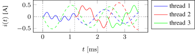
Figure 4: Time decomposition of the problem into three inhomogeneous problems with zero initial value (solid lines) and three homogeneous problems (dashed lines)

To test the algorithm on a more complex example a 2D cylindrical wave is simulated. The excitation is a line current in $z$-direction in the center of the domain $\Omega$ as shown in Figure 5.

Figure 5: Domain $\Omega$ of the wave problem with a hexahedral mesh

The discretization is obtained by FIT. A PEC boundary is assumed on the whole boundary $\partial\Omega$. The parameters of the discretization are $\Delta x=\Delta y=\Delta z=$1\text{\,}\mathrm{m}$$ and $n_{x}=n_{y}=21,\>n_{z}=2$ and the domain is filled with vacuum. The line current is a Gaussian function given by

$$i_{\text{L}}(t)=i_{\text{max}}e^{-4\left(\frac{t-\sigma_{t}}{\sigma_{t}}\right)^{2}}$$ (17)

with $i_{\text{max}}=$1\text{\,}\mathrm{A}$$ and $\sigma_{t}=$2\text{\times}{10}^{-8}\text{\,}\mathrm{s}$$.

The differential equation of this problem is given by (3) and (4) with $\bar{\mathbf{g}}(t)=-[\boldsymbol{0},\vbox{\halign{#\cr$\scriptscriptstyle\mathord{\frown}\mkern-0.2mu\cleaders\hbox{$\mkern-2.0mu\smash{-}\mkern-2.0mu$}\hfill\mkern-0.2mu$\crcr\kern-0.7pt\nointerlineskip\cr$\scriptscriptstyle\mathord{\frown}\mkern-0.2mu\cleaders\hbox{$\mkern-2.0mu\smash{-}\mkern-2.0mu$}\hfill\mkern-0.2mu$\crcr\kern-0.3pt\nointerlineskip\cr$\hfil\displaystyle{\rm\bf j}\hfil$\crcr}}]^{\top}$, with $\scriptscriptstyle\mathord{\frown}\mkern-0.2mu\cleaders\hbox{$\mkern-2.0mu\smash{-}\mkern-2.0mu$}\hfill\mkern-0.2mu$ $\scriptscriptstyle\mathord{\frown}\mkern-0.2mu\cleaders\hbox{$\mkern-2.0mu\smash{-}\mkern-2.0mu$}\hfill\mkern-0.2mu$ $\hfil\displaystyle{\rm\bf j}\hfil$ being the discretized line current (17).

The $\vbox{\halign{#\cr$\scriptscriptstyle\mathord{\frown}\mkern-0.2mu\cleaders\hbox{$\mkern-2.0mu\smash{-}\mkern-2.0mu$}\hfill\mkern-0.2mu$\crcr\kern-0.2pt\nointerlineskip\cr$\hfil\displaystyle{\rm\bf e}\hfil$\crcr}}_{z}$ component of the calculated wave can be seen in Figure 6 at $t=$4.4\text{\times}{10}^{-8}\text{\,}\mathrm{s}$$.

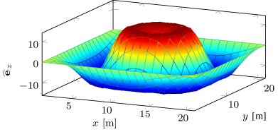
Figure 6: The $\vbox{\halign{#\cr$\scriptscriptstyle\mathord{\frown}\mkern-0.2mu\cleaders\hbox{$\mkern-2.0mu\smash{-}\mkern-2.0mu$}\hfill\mkern-0.2mu$\crcr\kern-0.2pt\nointerlineskip\cr$\hfil\displaystyle{\rm\bf e}\hfil$\crcr}}_{z}$ component of the wave at $t=$4.4\text{\times}{10}^{-8}\text{\,}\mathrm{s}$$

RK4 on the whole time interval and ParaExp (without approximation of the matrix exponential) on three threads are used to solve (3). Both approaches use a constant time step size $\Delta t=$2\text{\times}{10}^{-9}\text{\,}\mathrm{s}$$. With the obtained results, the energy in the domain is calculated using

$$W=\frac{1}{2}\left(\vbox{\halign{#\cr$\scriptscriptstyle\mathord{\frown}\mkern-0.2mu\cleaders\hbox{$\mkern-2.0mu\smash{-}\mkern-2.0mu$}\hfill\mkern-0.2mu$\crcr\kern-0.2pt\nointerlineskip\cr$\hfil\displaystyle{\rm\bf e}\hfil$\crcr}}^{\!\top}{\bf M}_{\varepsilon}\vbox{\halign{#\cr$\scriptscriptstyle\mathord{\frown}\mkern-0.2mu\cleaders\hbox{$\mkern-2.0mu\smash{-}\mkern-2.0mu$}\hfill\mkern-0.2mu$\crcr\kern-0.2pt\nointerlineskip\cr$\hfil\displaystyle{\rm\bf e}\hfil$\crcr}}+\vbox{\halign{#\cr$\scriptscriptstyle\mathord{\frown}\mkern-0.2mu\cleaders\hbox{$\mkern-2.0mu\smash{-}\mkern-2.0mu$}\hfill\mkern-0.2mu$\crcr\kern-0.2pt\nointerlineskip\cr$\hfil\displaystyle{\rm\bf h}\hfil$\crcr}}^{\!\top}{\bf M}_{\mu}\vbox{\halign{#\cr$\scriptscriptstyle\mathord{\frown}\mkern-0.2mu\cleaders\hbox{$\mkern-2.0mu\smash{-}\mkern-2.0mu$}\hfill\mkern-0.2mu$\crcr\kern-0.2pt\nointerlineskip\cr$\hfil\displaystyle{\rm\bf h}\hfil$\crcr}}\right).$$ (26)

The results are compared to a more accurate reference solution (i.e. the solution of the Runge-Kutta solver with a relative error tolerance of $1\text{\times}{10}^{-10}\text{\,}$). The comparison of the relative error of ParaExp and of the traditional RK4 method can be seen in Figure 7.

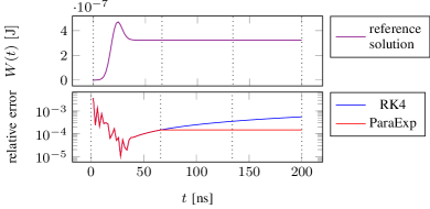
Figure 7: Reference solution (RK4 with a relative tolerance of $1\text{\times}{10}^{-10}\text{\,}$) for $W(t)$ and relative error of RK4 (with fixed time steps) and ParaExp

On the first interval both approaches coincide, afterwards the exponential is more accurate than the time stepper. However, in the current implementation this comes with higher costs since no approximation of the matrix exponential is used.

V Outlook

In the extended paper, we will discuss the application of the ParaExp method in more detail. The approximation of the action of the matrix exponential, the utilization of the Leapfrog scheme within ParaExp, and the numerical costs of the various methods will be investigated and compared. Finally the computational efficiency will be discussed using more complex examples.

References

• [1] J. Nievergelt, “Parallel methods for integrating ordinary differential equations,” Communications of the ACM, vol. 7, no. 12, pp. 731–733, 1964.
• [2] A. J. Christlieb, C. B. Macdonald, and B. W. Ong, “Parallel high-order integrators,” SIAM Journal on Scientific Computing, vol. 32, no. 2, pp. 818–835, 2010.
• [3] M. J. Gander and S. Güttel, “ParaExp: A parallel integrator for linear initial-value problems,” SIAM Journal on Scientific Computing, vol. 35, no. 2, pp. C123–C142, 2013.
• [4] J.-L. Lions, Y. Maday, and G. Turinici, “A ‘Parareal’ in time discretization of PDEs,” Comptes Rendus de l’Academie des Sciences Series I Mathematics, vol. 332, no. 7, pp. 661–668, 2001.
• [5] M. Minion, “A hybrid Parareal spectral deferred corrections method,” Communications in Applied Mathematics and Computational Science, vol. 5, no. 2, pp. 265–301, 2011.
• [6] W. L. Miranker and W. Liniger, “Parallel methods for the numerical integration of ordinary differential equations,” Mathematics of Computation, vol. 21, no. 99, pp. 303–320, 1967.
• [7] D. E. Womble, “A time-stepping algorithm for parallel computers,” SIAM Journal on Scientific and Statistical Computing, vol. 11, no. 5, pp. 824–837, 1990.
• [8] M. J. Gander and S. Vandewalle, “Analysis of the Parareal time-parallel time-integration method,” SIAM Journal on Scientific Computing, vol. 29, no. 2, pp. 556–578, 2007.
• [9] C. Farhat, J. Cortial, C. Dastillung, and H. Bavestrello, “Time-parallel implicit integrators for the near-real-time prediction of linear structural dynamic responses,” International Journal for Numerical Methods in Engineering, vol. 67, no. 5, pp. 697–724, 2006.
• [10] J. D. Jackson, Classical Electrodynamics.   Wiley, 1999.
• [11] T. Weiland, “A discretization model for the solution of Maxwell’s equations for six-component fields,” International Journal of Electronics and Communications, vol. 31, pp. 116–120, 1977.
• [12] ——, “Time domain electromagnetic field computation with finite difference methods,” International Journal of Numerical Modelling: Electronic Networks, Devices and Fields, vol. 9, no. 4, pp. 295–319, 1996.
• [13] A. Bossavit, Computational Electromagnetism. Variational Formulations, Complementarity, Edge Elements.   Academic Press, 1998.
• [14] A. H. Al-Mohy and N. J. Higham, “Computing the action of the matrix exponential, with an application to exponential integrators,” SIAM Journal on Scientific Computing, vol. 33, no. 2, pp. 488–511, 2011.
• [15] J. W. Eaton et al., “GNU Octave.” [Online]. Available: http://www.octave.org
• [16] T. Treichl and J. Corno, OdePkg, A Package for Solving Differential Equations with Octave.   Free Software Foundation. [Online]. Available: http://octave.sourceforge.net/odepkg/