A Comparison of Preconditioned Krylov Subspace
Methods for Large-Scale Nonsymmetric Linear Systems

Abstract

Preconditioned Krylov subspace (KSP) methods are widely used for solving large-scale sparse linear systems arising from numerical solutions of partial differential equations (PDEs). These linear systems are often nonsymmetric due to the nature of the PDEs, boundary or jump conditions, or discretization methods. While implementations of preconditioned KSP methods are usually readily available, it is unclear to users which methods are the best for different classes of problems. In this work, we present a comparison of some KSP methods, including GMRES, TFQMR, BiCGSTAB, and QMRCGSTAB, coupled with three classes of preconditioners, namely Gauss-Seidel, incomplete LU factorization (including ILUT, ILUTP, and multilevel ILU), and algebraic multigrid (including BoomerAMG and ML). Theoretically, we compare the mathematical formulations and operation counts of these methods. Empirically, we compare the convergence and serial performance for a range of benchmark problems from numerical PDEs in 2D and 3D with up to millions of unknowns and also assess the asymptotic complexity of the methods as the number of unknowns increases. Our results show that GMRES tends to deliver better performance when coupled with an effective multigrid preconditioner, but it is less competitive with an ineffective preconditioner due to restarts. BoomerAMG with proper choice of coarsening and interpolation techniques typically converges faster than ML, but both may fail for ill-conditioned or saddle-point problems while multilevel ILU tends to succeed. We also show that right preconditioning is more desirable. This study helps establish some practical guidelines for choosing preconditioned KSP methods and motivates the development of more effective preconditioners.
Keywords: Krylov subspace methods; preconditioners; multigrid methods; nonsymmetric systems; partial differential equations

Department of Applied Mathematics & Statistics and Institute for Advanced Computational Science,
Stony Brook University, Stony Brook, NY 11794, USA

1 Introduction

Preconditioned Krylov subspace (KSP) methods are widely used for solving large-scale sparse linear systems, especially those arising from numerical methods for partial differential equations (PDEs). For most modern applications, these linear systems are nonsymmetric due to various reasons, such as the multiphysics nature of the PDEs, sophisticated boundary or jump conditions, or the discretization methods themselves. For symmetric systems, conjugate gradient (CG) [34] and MINRES [43] are widely recognized as the best KSP methods [28]. However, the situation is far less clear for nonsymmetric systems. Various KSP methods have been developed, such as GMRES [52], CGS [56], QMR [30], TFQMR [29], BiCGSTAB [62], QMRCGSTAB [16], etc. Most of these methods are described in detail in textbooks such as [6, 51, 63], and their implementations are readily available in software packages, such as PETSc [5] and MATLAB [60]. However, each of these methods has its advantages and disadvantages. Therefore, it is difficult for practitioners to choose the proper methods for their specific applications. Moreover, a KSP method may perform well with one preconditioner but poorly with another. As a result, users often spend a significant amount of time to find a reasonable combination of the KSP methods and preconditioners through trial and error, and yet the final choice may still be far from optimal. Therefore, a systematic comparison of the preconditioned KSP methods is an important subject.

In the literature, various comparisons of KSP methods have been reported previously. In [41], Nachtigal, Reddy, and Trefethen presented some theoretical analysis and comparison of the convergence properties of CGN (CG on Normal equations), GMRES, and CGS, which were the leading methods for nonsymmetric systems in the early 1990s. They showed that the convergence of CGN is governed by singular values, whereas that of GMRES and CGS by eigenvalues and pseudo-eigenvalues, and each of these methods may significantly outperform the others for different matrices. Their work did not consider preconditioners. The work is also outdated because newer methods have been introduced since then, which are superior to CGN and CGS. In Saad’s textbook [51], some comparisons of various KSP methods, including GMRES, BiCGSTAB, QMR, and TFQMR, were given in terms of computational cost and storage requirements. The importance of preconditioners was emphasized, but no detailed comparison for the different combinations of the KSP methods and preconditioners was given. The same is also true for other textbooks, such as [63]. In terms of empirical comparison, Meister reported a comparison of a few preconditioned KSP methods for several inviscid and viscous flow problems [40]. His study focused on incomplete LU factorization as the preconditioner. Benzi and coworkers [9, 8] also compared a few preconditioners, also with a focus on incomplete factorization and their block variants. What were notably missing in these previous studies include the more advanced ILU preconditioners (such as multilevel ILU [12, 37]) and multigrid preconditioners, which have advanced significantly in recent years.

The goal of this work is to perform a systematic comparison and in turn establish some practical guidelines in choosing the best preconditioned KSP solvers. Our study is similar to the recent work of Feng and Saunders in [28], which compared CG and MINRES for symmetric systems. However, we focus on nonsymmetric systems with a heavier emphasis on preconditioners. We consider four KSP solvers, GMRES, TFQMR, BiCGSTAB and QMRCGSTAB. Among these, the latter three enjoy three-term recurrences. We also consider three classes of general-purpose preconditioners, namely Gauss-Seidel, incomplete LU factorization (including ILUT, ILUTP, and multilevel ILU), and algebraic multigrid (including variants of classical AMG and smoothed aggregation). Each of these KSP methods and preconditioners has its advantages and disadvantages. At the theoretical level, we compare the mathematical formulations, operation counts, and storage requirements of these methods. However, theoretical analysis alone is insufficient in establishing their suitability for different types of problems. The primary focus of this work is to compare the methods empirically in terms of convergence and serial performance for large linear systems. Our choice of comparing only serial performance is partially for keeping the focus on the mathematical properties of these methods, and partially due to the lack of efficient parallel implementation of ILU.

A systematic comparative study requires a comprehensive set of benchmark problems. Unfortunately, existing benchmark problems for nonsymmetric systems, such as those in the Matrix Market [11] and the UF Sparse Matrix Collection (a.k.a. the SuiteSparse Matrix Collection) [19], are generally too small to be representative of the large-scale problems in current engineering practice. They often also do not have the right-hand-side vectors, which can significantly affect the actual performance of KSP methods. To facilitate this comparison, we constructed a collection of benchmark systems ourselves from discretization methods for a range of PDEs in $2$-D and $3$-D. The sizes of these systems range from $10^{5}$ to $10^{7}$ unknowns, which are typical of modern industrial applications, and are much larger than most benchmark problems in previous studies. We also assess the asymptotic time complexity of different preconditioned KSP solvers with respect to the number of unknowns. To the best of our knowledge, this is the most comprehensive comparison of the preconditioned KSP solvers to date for large, sparse, nonsymmetric linear systems in terms of convergence rate, serial performance, and asymptotic complexity. Our results also show that BoomerAMG in hypre [25], which is an extension of classical AMG, typically converges faster than Trillions/ML [31], which is a variant of smoothed-aggregation AMG. However, it is important to choose the coarsening and interpolation techniques in BoomerAMG, and we observe that HMIS+FF1 tends to outperform the default options in both older and newer versions of hypre. However, both AMG methods tend to fail for very ill-conditioned systems or saddle-point-like problems, while multilevel ILU, and also ILUTP to some extent, tend to succeed. We also observed that right preconditioning is, in general, more reliable than left preconditioning for large-scale systems. Our results help establish some practical guidelines for choosing preconditioned KSP methods. They also motivate the further development of more effective, scalable, and robust multigrid preconditioners.

The remainder of the paper is organized as follows. In Section 2, we review some background knowledge of numerical PDEs, KSP methods, and preconditioners. In Section 3, we outline a few KSP methods and compare their main properties in terms of asymptotic convergence, the number of operations per iteration, and the storage requirement. This theoretical background will help us predict the relative performance of the various methods and interpret the numerical results. In Section 4, we describe the benchmark problems. In Section 5, we present numerical comparisons of the preconditioned KSP methods. Finally, Section 6 concludes the paper with some practical recommendations and a discussion on future work.

2 Background

In this section, we give a general overview of Krylov subspace methods and preconditioners for solving a nonsymmetric linear system

$$\boldsymbol{A}\boldsymbol{x}=\boldsymbol{b},$$ (1)

where $\boldsymbol{A}\in\mathbb{R}^{n\times n}$ is large, sparse, nonsymmetric, and nonsingular, and $\boldsymbol{b}\in\mathbb{R}{}^{n}$. These systems typically arise from PDE discretizations. We consider only real matrices, because they are more common in applications. However, all the methods apply to complex matrices, by replacing the matrix transposes with the conjugate transposes. We focus on the Krylov subspaces and the procedure in constructing the basis vectors of the subspaces, which are often the determining factors in the overall performance of different types of KSP methods. We defer more detailed discussions and analysis of the individual methods to Section 3.

2.1 Nonsymmetric Systems from Numerical PDEs

This work is concerned of solving nonsymmetric systems from discretization of PDEs. It is important to understand the origins of these systems, especially of their nonsymmetric structures. Consider an abstract but general linear, time-independent scalar PDE over $\Omega\subset\mathbb{R}^{d}$,

$$\mathcal{L}u(\boldsymbol{x})=f(\boldsymbol{x}),$$ (2)

with Dirichlet or Neumann boundary conditions (BCs) over $\Gamma_{D}$ and $\Gamma_{N}$, respectively, where $d=2$ or $3$, and $\mathcal{L}$ is a linear differential operator, and $f$ is a known source term. A specific and yet quite general example is the second-order boundary value problem

$$-\boldsymbol{\nabla}\cdot(\mu\boldsymbol{\nabla}u)+\boldsymbol{\nu}\cdot\boldsymbol{\nabla}u+\omega^{2}u =f\quad\,\,\,\,\,\text{ in }\Omega,$$ (3)

$$u =u_{D}\quad\text{ on }\Gamma_{D},$$ (4)

$$\boldsymbol{n}\cdot\boldsymbol{\nabla}u =g\quad\,\,\,\,\text{ on }\Gamma_{N},$$ (5)

for which $\mathcal{L}u=-\boldsymbol{\nabla}\cdot(\mu\boldsymbol{\nabla}u)+\boldsymbol{\nu}\cdot\boldsymbol{\nabla}u+\omega^{2}u$, where $\mu$ is scalar field, $\boldsymbol{\nu}$ is a vector field, $\omega$ is a scalar, and $\boldsymbol{n}$ denotes outward normal to $\Gamma_{N}$. If $\omega=0$, then it is a convection-diffusion (a.k.a. advection-diffusion) equation, where $\mu$ corresponds to a diffusion coefficient, and $\boldsymbol{\nu}$ corresponds to a velocity field. If $\boldsymbol{\nu}=\boldsymbol{0}$, then it is a Helmholtz equation, and $\omega$ typically corresponds to a wavenumber or frequency.

For ease of discussion, we express the PDE discretization methods using a general notion of weighted residuals. In particular, consider a set of test (a.k.a. weight) functions $\{\psi_{i}(\boldsymbol{x})\}$. The PDE (2) is then converted into a set of integral equations

$$\int_{\Omega}\mathcal{L}u(\boldsymbol{x})\,\psi_{i}\,d\boldsymbol{x}=\int_{\Omega}f(\boldsymbol{x})\,\psi_{i}\,d\boldsymbol{x}.$$ (6)

To discretize the equations fully, consider a set of basis functions $\{\phi_{ij}(\boldsymbol{x})\}$ corresponding to each test function, and let $u_{i}^{h}\approx\sum_{i}u_{i}\phi_{ij}$ be a local approximation to $u$ with respect to $\psi_{i}$. Then, we obtain a linear system

$$\boldsymbol{A}\boldsymbol{u}=\boldsymbol{b},$$ (7)

where

$$a_{ij}=\int_{\Omega}\mathcal{L}\phi_{ij}(\boldsymbol{x})\,\psi_{i}(\boldsymbol{x})\,d\boldsymbol{x}\mbox{ \,\,\ and\,\,\ }b_{i}=\int_{\Omega}f(\boldsymbol{x})\,\psi_{i}(\boldsymbol{x})\,d\boldsymbol{x}.$$ (8)

This system may be further modified to apply boundary conditions. In general, the test and basis functions have local support, and therefore $\boldsymbol{A}$ is in general sparse.

In finite element methods (FEM) and their variants, the test functions are typically piecewise linear or higher-degree polynomials, such as hat functions, and the same set of basis functions $\{\phi_{j}(\boldsymbol{x})\}$ is used regardless of $\psi_{i}$. Since the test and basis functions are weakly differentiable in FEM, integration by parts is used to reduce the elliptic operator in $\mathcal{L}$ to a symmetric first-order differential operator in the interior of the domain; see e.g. [24] for details of FEM. If $\{\phi_{i}\}=\{\psi_{i}\}$, the FEM is a Galerkin method, and $\boldsymbol{A}$ is nonsymmetric if $\boldsymbol{\nu}\neq 0$ in (3). If $\{\phi_{i}\}\neq\{\psi_{i}\}$, the FEM is a Petrov-Galerkin method, and $\boldsymbol{A}$ is always nonsymmetric.

In finite difference methods (FDM), the test functions are Dirac delta functions at the nodes, and at each node a different set of polynomial basis functions is constructed from the interpolation over its stencil; see e.g. [57] for details of FDM. On uniform structured grids, FDM with centered differences leads to symmetric matrices for Helmholtz equations with Dirichlet BCs. However, the matrices are in general nonsymmetric for PDEs with Neumann BCs, FDM on nonuniform or curvilinear grids, or higher-order FDM.

While finite differences were traditionally limited to structured or curvilinear meshes, they are generalized to unstructured meshes or point clouds in the so-called generalized finite difference methods (GFDM); see e.g. [7]. Like FDM, at each node GFDM has a set of polynomial basis functions over its stencil, which are constructed from least squares fittings instead of interpolation. The matrices from GFDM are always nonsymmetric. A closely method is AES-FEM [18], of which the test functions are similar to those of FEM but the basis functions are similar to those of GFDM. The linear systems from AES-FEM are also nonsymmetric.

The model problem (2) is a scalar BVP, but it can be generalized to vector-valued systems of PDEs. In this setting, $u$ is replaced by a vector field, and $\mu$, $\boldsymbol{\nu}$ and $\omega^{2}$ are replaced by tensors, which may be determined by additional unknowns. Systems of PDEs, such as Stokes equations, lead to saddle-point-like problems, of which the linear systems have large diagonal blocks. For time-dependent problems, such as hyperbolic or advection-diffusion problems, nonsymmetric linear systems may arise due to finite-element spatial discretization or implicit time stepping. In particular, hyperbolic problems are often solved using the discontinuous Galerkin (DG) or finite volume (FVM) or methods, of which the test functions are local polynomials over each element (or cell). A different set of polynomial basis functions are used per element (or cell), with flux reconstruction and flux limiters along element (or cell) boundaries. These methods lead to nonsymmetric systems if implicit time stepping is used.

2.2 Krylov Subspaces

For large-scale sparse linear systems, Krylov-subspace methods are among the most powerful techniques. Given a matrix $\boldsymbol{A}\in\mathbb{R}^{n\times n}$ and a vector $\boldsymbol{v}\in\mathbb{R}^{n}$, the $k$th Krylov subspace generated by them, denoted by $\mathcal{K}_{k}(\boldsymbol{A},\boldsymbol{v})$, is given by

$$\mathcal{K}_{k}(\boldsymbol{A},\boldsymbol{v})=\mbox{span}\{\boldsymbol{v},\boldsymbol{A}\boldsymbol{v},\boldsymbol{A}^{2}\boldsymbol{v},\dots,\boldsymbol{A}^{k-1}\boldsymbol{v}\}.$$ (9)

To solve (1), let $\boldsymbol{x}_{0}$ be some initial guess to the solution, and $\boldsymbol{r}_{0}=\boldsymbol{b}-\boldsymbol{A}\boldsymbol{x}_{0}$ is the initial residual vector. A Krylov subspace method incrementally finds approximate solutions within $\mathcal{K}_{k}(\boldsymbol{A},\boldsymbol{v})$, sometimes through the aid of another Krylov subspace $\mathcal{K}_{k}(\boldsymbol{A}^{T},\boldsymbol{w})$, where $\boldsymbol{v}$ and $\boldsymbol{w}$ typically depend on $\boldsymbol{r}_{0}$. To construct the basis of the subspace $\mathcal{K}(\boldsymbol{A},\boldsymbol{v})$, two procedures are commonly used: the (restarted) Arnoldi iteration [3], and the bi-Lanczos iteration [36, 63] (a.k.a. Lanczos biorthogonalization [51] or tridiagonal biorthogonalization [61]).

2.2.1 The Arnoldi Iteration.

The Arnoldi iteration is a procedure for constructing orthogonal basis of the Krylov subspace $\mathcal{K}(\boldsymbol{A},\boldsymbol{v})$. Starting from a unit vector $\boldsymbol{q}_{1}=\boldsymbol{v}/\|\boldsymbol{v}\|$, it iteratively constructs

$$\boldsymbol{Q}_{k+1}=[\boldsymbol{q}_{1}\mid\boldsymbol{q}_{2}\mid\dots\mid\boldsymbol{q}_{k}\mid\boldsymbol{q}_{k+1}]$$ (10)

with orthonormal columns by solving

$$h_{k+1,k}\boldsymbol{q}_{k+1}=\boldsymbol{A}\boldsymbol{q}_{k}-h_{1k}\boldsymbol{q}_{1}-\cdots-h_{kk}\boldsymbol{q}_{k},$$ (11)

where $h_{ij}=\boldsymbol{q}_{i}^{T}\boldsymbol{A}\boldsymbol{q}_{j}$ for $j\leq i$, and $h_{k+1,k}=\|\boldsymbol{A}\boldsymbol{q}_{k}-h_{1k}\boldsymbol{q}_{1}-\cdots-h_{kk}\boldsymbol{q}_{k}\|$, i.e., the norm of the right-hand side of (11). This is analogous to Gram-Schmidt orthogonalization. If $\mathcal{K}_{k}\neq\mathcal{K}_{k-1}$, then the columns of $\boldsymbol{Q}_{k}$ form an orthonormal basis of $\mathcal{K}_{k}(\boldsymbol{A},\boldsymbol{v})$, and

$$\boldsymbol{A}\boldsymbol{Q}_{k}=\boldsymbol{Q}_{k+1}\tilde{\boldsymbol{H}}_{{}_{k}},$$ (12)

where $\tilde{\boldsymbol{H}}_{{}_{k}}$ is a $(k+1)\times k$ upper Hessenberg matrix, whose entries $h_{ij}$ are those in (11) for $i\leq j+1$, and $h_{ij}=0$ for $i>j+1$.

The KSP method GMRES [52] is based on the Arnoldi iteration, with $\boldsymbol{v}=\boldsymbol{r}_{0}$. If $\boldsymbol{A}$ is symmetric, the Hessenberg matrix $\tilde{\boldsymbol{H}}_{{}_{k}}$ reduces to a tridiagonal matrix, and the Arnoldi iteration reduces to the Lanczos iteration. The Lanczos iteration enjoys a three-term recurrence. In contrast, the Arnoldi iteration has a $k$-term recurrence, so its computational cost increases as $k$ increases. For this reason, one typically needs to restart the Arnoldi iteration for large systems (e.g., after every 30 iterations) to build a new Krylov subspace from $\boldsymbol{v}=\boldsymbol{r}_{k}$ at restart. Unfortunately, the restart may undermine the convergence of the KSP methods [52].

2.2.2 The Bi-Lanczos Iteration.

The bi-Lanczos iteration, also known as Lanczos biorthogonalization or tridiagonal biorthogonalization, offers an alternative for constructing the basis of the Krylov subspaces of $\mathcal{K}(\boldsymbol{A},\boldsymbol{v})$. Unlike Arnoldi iterations, the bi-Lanczos iterations enjoy a three-term recurrence. However, the basis will no longer be orthogonal, and we need to use two matrix-vector multiplications per iteration, instead of just one.

The bi-Lanczos iterations can be described as follows. Starting from the vector $\boldsymbol{v}_{1}=\boldsymbol{v}/\|\boldsymbol{v}\|$, we iteratively construct

$$\boldsymbol{V}_{k+1}=[\boldsymbol{v}_{1}\mid\boldsymbol{v}_{2}\mid\dots\mid\boldsymbol{v}_{k}\mid\boldsymbol{v}_{k+1}],$$ (13)

by solving

$$\beta_{k}\boldsymbol{v}_{k+1}=\boldsymbol{A}\boldsymbol{v}_{k}-\gamma_{k-1}\boldsymbol{v}_{k-1}-\alpha_{k}\boldsymbol{v}_{k},$$ (14)

analogous to (11). If $\mathcal{K}_{k}\neq\mathcal{K}_{k-1}$, then the columns of $\boldsymbol{V}_{k}$ form a basis of $\mathcal{K}_{k}(\boldsymbol{A},\boldsymbol{v})$, and

$$\boldsymbol{A}\boldsymbol{V}_{k}=\boldsymbol{V}_{k+1}\tilde{\boldsymbol{T}}_{{}_{k}},$$ (15)

where

$$\tilde{\boldsymbol{T}}_{{}_{k}}=\begin{bmatrix}\alpha_{1}&\gamma_{1}\\ \beta_{1}&\alpha_{2}&\gamma_{2}\\ &\beta_{2}&\alpha_{3}&\ddots\\ &&\ddots&\ddots&\gamma_{k-1}\\ &&&\beta_{k-1}&\alpha_{k}\\ &&&&\beta_{k}\end{bmatrix}$$ (16)

is a $(k+1)\times k$ tridiagonal matrix. To determine the $\alpha_{i}$ and $\gamma_{i}$, we construct another Krylov subspace $\mathcal{K}(\boldsymbol{A}^{T},\boldsymbol{w})$, whose basis is given by the column vectors of

$$\boldsymbol{W}_{k+1}=[\boldsymbol{w}_{1}\mid\boldsymbol{w}_{2}\mid\dots\mid\boldsymbol{w}_{k}\mid\boldsymbol{w}_{k+1}],$$ (17)

subject to the biorthogonality condition

$$\boldsymbol{W}_{k+1}^{T}\boldsymbol{V}_{k+1}=\boldsymbol{V}_{k+1}^{T}\boldsymbol{W}_{k+1}=\boldsymbol{I}_{k+1}.$$ (18)

Since

$$\boldsymbol{W}_{k+1}^{T}\boldsymbol{A}\boldsymbol{V}_{k}=\boldsymbol{W}_{k+1}^{T}\boldsymbol{V}_{k+1}\tilde{\boldsymbol{T}}_{{}_{k}}=\tilde{\boldsymbol{T}}_{{}_{k}},$$ (19)

it then follows that

$$\alpha_{k}=\boldsymbol{w}_{k}^{T}\boldsymbol{A}\boldsymbol{v}_{k}.$$ (20)

Suppose $\boldsymbol{V}=\boldsymbol{V}_{n}$ and $\boldsymbol{W}=\boldsymbol{W}_{n}=\boldsymbol{V}^{-T}$ form complete basis vectors of $\mathcal{K}_{n}(\boldsymbol{A},\boldsymbol{v})$ and $\mathcal{K}_{n}(\boldsymbol{A}^{T},\boldsymbol{w})$, respectively. Let $\boldsymbol{T}=\boldsymbol{V}^{-1}\boldsymbol{A}\boldsymbol{V}$ and $\boldsymbol{S}=\boldsymbol{T}^{T}$. Then,

$$\boldsymbol{W}^{-1}\boldsymbol{A}^{T}\boldsymbol{W}=\boldsymbol{V}^{T}\boldsymbol{A}^{T}\boldsymbol{V}^{-T}=\boldsymbol{T}^{T}=\boldsymbol{S},$$ (21)

and

$$\boldsymbol{A}^{T}\boldsymbol{W}_{k}=\boldsymbol{W}_{k+1}\tilde{\boldsymbol{S}}_{{}_{k}},$$ (22)

where $\tilde{\boldsymbol{S}}_{k}$ is the leading $(k+1)\times k$ submatrix of $\boldsymbol{S}$. Therefore,

$$\gamma_{k}\boldsymbol{w}_{k+1}=\boldsymbol{A}^{T}\boldsymbol{w}_{k}-\beta_{k-1}\boldsymbol{w}_{k-1}-\alpha_{k}\boldsymbol{w}_{k}.$$ (23)

Starting from $\boldsymbol{v}_{1}$ and $\boldsymbol{w}_{1}$ with $\boldsymbol{v}_{1}^{T}\boldsymbol{w}_{1}=1$, and let $\beta_{0}=\gamma_{0}=1$ and $\boldsymbol{v}_{0}=\boldsymbol{w}_{0}=\boldsymbol{0}$. Then, $\alpha_{k}$ is uniquely determined by (20), and $\beta_{k}$ and $\gamma_{k}$ are determined by (14) and (23) by up to scalar factors, subject to $\boldsymbol{v}_{k+1}^{T}\boldsymbol{w}_{k+1}=1$. A typical choice is to scale the right-hand sides of (14) and (23) by scalars of the same modulus [51, p. 230].

If $\boldsymbol{A}$ is symmetric and $\boldsymbol{v}_{1}=\boldsymbol{w}_{1}=\boldsymbol{v}/\|\boldsymbol{v}\|$, then the bi-Lanczos iteration reduces to the classical Lanczos iteration for symmetric matrices. Therefore, it can be viewed as a different generalization of the Lanczos iteration to nonsymmetric matrices. Unlike the Arnoldi iteration, the cost of bi-Lanczos iteration is fixed per iteration, so no restart is ever needed. Some KSP methods, in particular BiCG [26] and QMR [30], are based on bi-Lanczos iterations. A potential issue of bi-Lanczos iteration is that it may suffer from breakdown if $\boldsymbol{v}_{k+1}^{T}\boldsymbol{w}_{k+1}=0$ or near breakdown if $\boldsymbol{v}_{k+1}^{T}\boldsymbol{w}_{k+1}\approx 0$. These can be resolved by a look-ahead strategy to build a block-tridiagonal matrix $\boldsymbol{T}$. Fortunately, breakdowns are rare, so look-ahead is rarely implemented.

A disadvantage of the bi-Lanczos iteration is that it requires the multiplication with $\boldsymbol{A}^{T}$. Although $\boldsymbol{A}^{T}$ is in principle available in most applications, multiplication with $\boldsymbol{A}^{T}$ leads to additional difficulties in performance optimization and preconditioning. Fortunately, in bi-Lanczos iteration, $\boldsymbol{V}_{k}$ can be computed without forming $\boldsymbol{W}_{k}$ and vice versa. This observation leads to the transpose-free variants of the KSP methods, such as TFQMR [29], which is a transpose-free variant of QMR, and CGS [56], which is a transpose-free variant of BiCG. Two other examples include BiCGSTAB [62], which is more stable than CGS, and QMRCGSTAB [16], which is a hybrid of QMR and BiCGSTAB, with smoother convergence than BiCGSTAB. These transpose-free methods enjoy three-term recurrences and require two multiplications with $\boldsymbol{A}$ per iteration. Note that there is not a unique transpose-free bi-Lanczos iteration. There are primarily two types, used by CGS and QMR, and by BiCGSTAB and QMRCGSTAB, respectively. We will address them in more detail in Section 3.

2.2.3 Comparison of the Iteration Procedures.

Table 1: Comparisons of KSP methods based on Krylov subspaces and iteration procedures.

Method	Iteration	Matrix-Vector Prod.		Recurrence
		AT	A

GMRES [52]& Arnoldi 0 1 $k$ BiCG [26] bi-Lanczos 1 1 3 QMR [30] CGS [56] transpose-free bi-Lanczos 1      0      2 TFQMR [29] BiCGSTAB [62] transpose-free bi-Lanczos 2 QMRCGSTAB [16]

Both the Arnoldi iteration and the bi-Lanczos iteration are based on the Krylov subspace $\mathcal{K}(\boldsymbol{A},\boldsymbol{r}_{0})$. However, these iteration procedures have very different properties, which are inherited by their corresponding KSP methods, as summarized in Table 2.2.3. These properties, for the most part, determine the cost per iteration of the KSP methods. For KSP methods based on the Arnoldi iteration, at the $k$th iteration the residual $\boldsymbol{r}_{k}=\mathcal{P}_{k}(\boldsymbol{A})\boldsymbol{r}_{0}$ for some degree-$k$ polynomial $\mathcal{P}_{k}$, so the asymptotic convergence rates primarily depend on the eigenvalues and the generalized eigenvectors in the Jordan form of $\boldsymbol{A}$ [41, 51]. For methods based on transpose-free bi-Lanczos, in general $\boldsymbol{r}_{k}=\hat{\mathcal{P}}_{k}(\boldsymbol{A})\boldsymbol{r}_{0}$, where $\hat{\mathcal{P}}_{k}$ is a polynomial of degree $2k$. Therefore, the convergence of these methods also depends on the eigenvalues and generalized eigenvectors of $\boldsymbol{A}$, but at different asymptotic rates. Typically, the reduction of error in one iteration of a bi-Lanczos-based KSP method is approximately equal to that of two iterations in an Arnoldi-based KSP method. Since the Arnoldi iteration requires only one matrix-vector multiplication per iteration, compared to two per iteration for the bi-Lanczos iteration, the costs of different KSP methods are comparable in terms of the number of matrix-vector multiplications.

Theoretically, the Arnoldi iteration is more robust because of its use of orthogonal basis, whereas the bi-Lanczos iteration may breakdown if $\boldsymbol{v}_{k+1}^{T}\boldsymbol{w}_{k+1}=0$. However, the Arnoldi iteration typically requires restarts, which can undermine convergence. In general, if the iteration count is small compared to the average number of nonzeros per row, the methods based on the Arnoldi iteration may be more efficient; if the iteration count is large, the cost of orthogonalization in Arnoldi iteration may become higher than that of bi-Lanczos iteration. For these reasons, conflicting results are often reported in the literature. However, the apparent disadvantages of each KSP method may be overcome by effective preconditioners: For Arnoldi iterations, if the KSP method converges before restart is needed, then it may be the most effective method; for bi-Lanczos iterations, if the KSP method converges before any breakdown, it is typically more robust than the methods based on restarted Arnoldi iterations. We will review the preconditioners in the next subsection.

Note that some KSP methods use a Krylov subspace other than $\mathcal{K}(\boldsymbol{A},\boldsymbol{r}_{0})$. The most notable examples are LSQR [44] and LSMR [27], which use the Krylov subspace $\mathcal{K}(\boldsymbol{A}^{T}\boldsymbol{A},\boldsymbol{A}^{T}\boldsymbol{r}_{0})$. These methods are mathematically equivalent to applying CG or MINRES to the normal equation, respectively, but with better numerical properties than CGN. An advantage of these methods is that they apply to least squares systems without modification. However, they are not transpose-free, they tend to converge slowly for square linear systems, and they require special preconditioners. For these reasons, we do not include them in this study.

2.3 Preconditioners

The convergence of KSP methods can be improved significantly by the use of preconditioners. Various preconditioners have been proposed for Krylov subspace methods over the past few decades. It is virtually impossible to consider all of them. For this comparative study, we focus on three classes of preconditioners, which are representative for the state-of-the-art “black-box” preconditioners: Gauss-Seidel, incomplete LU factorization, and algebraic multigrid.

2.3.1 Left versus Right Preconditioning.

Roughly speaking, a preconditioner is a matrix or transformation $\boldsymbol{M}$, whose inverse $\boldsymbol{M}^{-1}$ approximates $\boldsymbol{A}^{-1}$, and $\boldsymbol{M}^{-1}\boldsymbol{v}$ can be computed efficiently. For nonsymmetric linear systems, a preconditioner may be applied either to the left or the right of $\boldsymbol{A}$. With a left preconditioner, instead of solving (1), one solves the linear system

$$\boldsymbol{M}^{-1}\boldsymbol{A}\boldsymbol{x}=\boldsymbol{M}^{-1}\boldsymbol{b}$$ (24)

by utilizing the Krylov subspace $\mathcal{K}(\boldsymbol{M}^{-1}\boldsymbol{A},\boldsymbol{M}^{-1}\boldsymbol{b})$ instead of $\mathcal{K}(\boldsymbol{A},\boldsymbol{b})$. For a right preconditioner, one solves the linear system

$$\boldsymbol{A}\boldsymbol{M}^{-1}\boldsymbol{y}=\boldsymbol{b}$$ (25)

by utilizing the Krylov subspace $\mathcal{K}(\boldsymbol{A}\boldsymbol{M}^{-1},\boldsymbol{b})$, and then $\boldsymbol{x}=\boldsymbol{M}^{-1}\boldsymbol{y}$. The convergence of a preconditioned KSP method is then determined by the eigenvalues of $\boldsymbol{M}^{-1}\boldsymbol{A}$, which are the same as those of $\boldsymbol{A}\boldsymbol{M}^{-1}$, as well as their generalized eigenvectors. Qualitatively, $\boldsymbol{M}$ is a good preconditioner if $\boldsymbol{M}^{-1}\boldsymbol{A}$ (or $\boldsymbol{A}\boldsymbol{M}^{-1}$ for right preconditioning) is not too far from normal and its eigenvalues are more clustered than those of $\boldsymbol{A}$ [61]. However, this is more useful as a guideline for developers of preconditioners, rather than for users.

Although the left and right-preconditioners have similar asymptotic behavior, they can behave drastically differently in practice. It is advisable to use right, instead of left, preconditioners for two reasons. First, the termination criterion of a Krylov subspace method is typically based on the norm of the residual of the preconditioned system, which may differ significantly from the true residual. Figure 1 shows two examples, where the norms of the preconditioned residuals are significantly larger and smaller than the true residuals, respectively; we will explain these matrices in Section 4. Second, if the iteration terminates with a relatively large residual $\boldsymbol{r}$, then the error of the solution is bounded by

$$\left\|\delta\boldsymbol{x}\right\|\leq\left\|\boldsymbol{M}\boldsymbol{A}^{-1}\right\|\left\|\boldsymbol{M}^{-1}\boldsymbol{r}\right\|\leq\kappa(\boldsymbol{M})\left\|\boldsymbol{A}^{-1}\right\|\left\|\boldsymbol{r}\right\|,$$ (26)

which may differ significantly from $\left\|\boldsymbol{A}^{-1}\right\|\left\|\boldsymbol{r}\right\|$ if $\kappa(\boldsymbol{M})\gg 1$. The stability analysis of PDE discretization typically depends on the boundedness of $\left\|\boldsymbol{A}^{-1}\right\|$ in (7), so one should not change the residual unless the preconditioner is derived based on a priori knowledge of the PDE discretization. One could overcome these issues by computing the true residual $\left\|\boldsymbol{r}\right\|$ at each step, but it would incur additional costs with a left preconditioner. Since the preconditioners that we consider are algebraic in nature, we use only right preconditioners in this study.

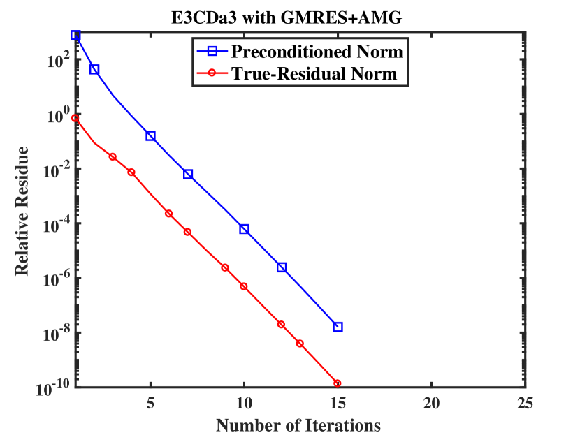
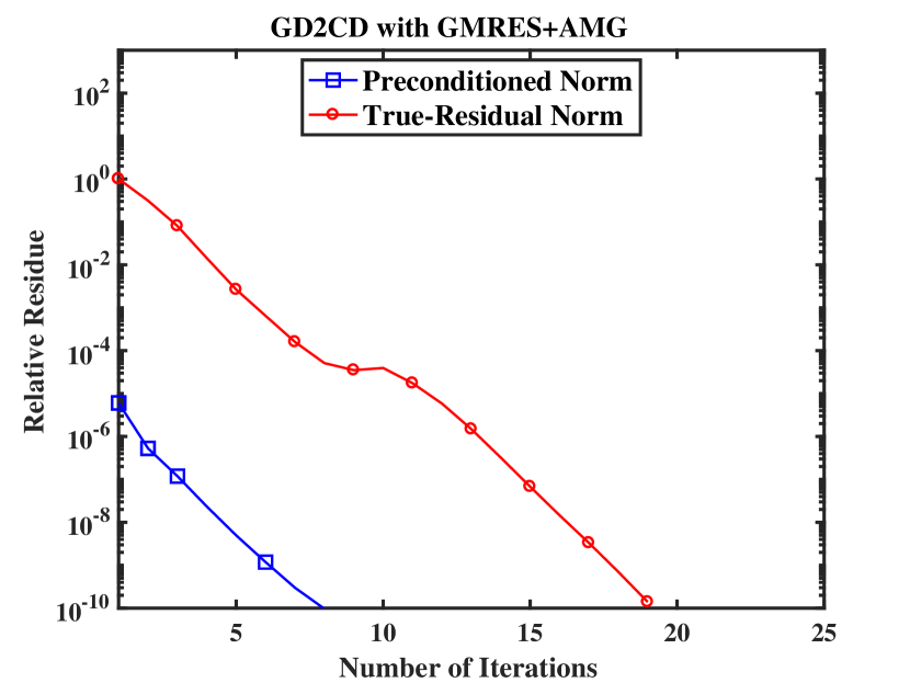
Figure 1: Examples where left preconditioners lead to large discrepancies of preconditioned and true residuals by orders of magnitude and in turn delayed (left) or premature termination (right).

Note that in the so-called symmetric preconditioners, the Cholesky factorization of $\boldsymbol{M}^{-1}$ is applied symmetrically to both the left and right of $\boldsymbol{A}$. A well-known example is the symmetric successive over-relaxation (SSOR) [33]. Such preconditioners preserve symmetry for symmetric matrices. However, since they also alter the norm of the residual and our focus is on nonsymmetric matrices, we do not consider symmetric preconditioners in this study.

2.3.2 Gauss-Seidel and SOR.

Gauss-Seidel and its generalization SOR (successive over-relaxation) are some of the simplest preconditioners. Based on stationary iterative methods, Gauss-Seidel and SOR are relatively easy to implement, require virtually no setup time (at least in serial), and are sometimes fairly effective. Therefore, they are often good choices if one needs to implement a preconditioner from scratch.

Consider the partitioning $\boldsymbol{A}=\boldsymbol{D}+\boldsymbol{L}+\boldsymbol{U}$, where $\boldsymbol{D}$ is the diagonal of $\boldsymbol{A}$, $\boldsymbol{L}$ is the strictly lower triangular part, and $\boldsymbol{U}$ is the strictly upper triangular part. Given $\boldsymbol{x}_{k}$ and $\boldsymbol{b}$, the Gauss-Seidel method computes a new approximation to $\boldsymbol{x}_{k+1}$ as

$$\boldsymbol{x}_{k+1}=(\boldsymbol{D}+\boldsymbol{L})^{-1}(\boldsymbol{b}-\boldsymbol{U}\boldsymbol{x}_{k}).$$ (27)

SOR generalizes Gauss-Seidel by introducing a relaxation parameter $\omega$. It computes $\boldsymbol{x}_{k+1}$ as

$$\boldsymbol{x}_{k+1}=(\boldsymbol{D}+\omega\boldsymbol{L})^{-1}\left(\omega\left(\boldsymbol{b}-\boldsymbol{U}\boldsymbol{x}_{k}\right)+(1-\omega)\boldsymbol{D}\boldsymbol{x}_{k}\right).$$ (28)

When $\omega=1$, SOR reduces to Gauss-Seidel; when $\omega>1$ and $\omega<1$, it corresponds to over-relaxation and under-relaxation, respectively. We choose to include Gauss-Seidel instead of SOR in our comparison, because it is parameter free, and an optimal choice of $\omega$ in SOR is problem dependent. Another related preconditioner is the Jacobi or diagonal preconditioner, which is less effective than Gauss-Seidel. A limitation of Gauss-Seidel, also shared by Jacobi and SOR, is that the diagonal entries of $\boldsymbol{A}$ must be nonzero.

2.3.3 Incomplete LU Factorization.

Incomplete LU factorization (ILU) performs an approximate factorization

$$\boldsymbol{A}\approx\tilde{\boldsymbol{L}}\tilde{\boldsymbol{U}},$$ (29)

where $\tilde{\boldsymbol{L}}$ and $\tilde{\boldsymbol{U}}$ are far sparser than those in the LU factorization of $\boldsymbol{A}$. This approximate factorization is typically computed in a preprocessing step. In the preconditioned Krylov solver, $\boldsymbol{M}^{-1}\boldsymbol{y}$ is computed by forward solve $\boldsymbol{z}=\tilde{\boldsymbol{L}}^{-1}\boldsymbol{y}$ and then back substitution $\tilde{\boldsymbol{U}}^{-1}\boldsymbol{z}$.

There are several variants of ILU factorization. In its simplest form, ILU does not introduce any fill, so that $\tilde{\boldsymbol{L}}$ and $\tilde{\boldsymbol{U}}$ preserve the sparsity patterns of the lower and upper triangular parts of $\boldsymbol{A}$, respectively. This approach is often referred to as ILU0 or ILU(0). ILU0 may be extended to preserve some of the fills based on their levels in the elimination tree. This is often referred to as ILU$(k)$, which zeros out all the fills of level $k+1$ or higher. In addition, ILU$(k)$ may be further combined with thresholding on the numerical values, resulting in ILU with dual thresholding (ILUT) [49]. Most implementations of ILU, such as those in PETSc and hypre, use some variants of ILUT, where PETSc also allows the user to control the number of fills.

A serious issue with ILUT is that it may breakdown if there are many zeros in the diagonal. This issue can be mitigated by pre-permuting the matrix, but it may still fail in practice for saddle-point-like problems. A more effective approach is to use partial pivoting, which results in the so-called ILUTP [51]. The ILU implementations in MATLAB [60], SPARSKIT [50], and SuperLU [37], for example, are based on ILUTP.

A major drawback of ILUTP is that the number of nonzeros in the $\tilde{\boldsymbol{L}}$ and $\tilde{\boldsymbol{U}}$ factors may grow superlinearly with respect to the original number of nonzeros if the drop tolerance is small. This leads to superlinear growth of setup times and solve times. However, a small drop tolerance may be needed for robustness, especially for very large sparse systems. As a result, parameter tuning for ILUTP may become an impossible task. This problem is mitigated by the multilevel ILU, or MILU for short. Unlike ILUTP, MILU uses diagonal pivoting instead of partial pivoting, and it permutes rows and columns that would have led to ill-conditioned $\tilde{\boldsymbol{L}}$ and $\tilde{\boldsymbol{U}}$ to the end and delays factorizing them [12]. This approach leads to much better robustness with a relatively small number of fills. A robust, serial implementation of MILU is available in ILUPACK [13]. Typically, MILU scales linearly with respect to the original number of nonzeros, so it is effective for large sparse linear systems, especially in serial. We will report some numerical comparisons of different variants of ILU in Section 5.2.

2.3.4 Algebraic Multigrid.

Multigrid methods, including geometric multigrid (GMG) and algebraic multigrid (AMG), are the most sophisticated preconditioners. These methods accelerate stationary iterative methods (or more precisely, the so-called smoothers in multigrid methods) by constructing a series of coarser representations. The key difference between GMG and AMG is the coarsening strategies and the associated prolongation (a.k.a. interpolation) and restriction (a.k.a. projection) operators between different levels. Compared to Gauss-Seidel and ILU, multigrid preconditioners, especially GMG, are far more difficult to implement. Fortunately, AMG preconditioners are more readily accessible through software libraries. Similar to ILU, AMG typically requires a significant amount of pre-processing time. Computationally, AMG is more expensive than Gauss-Seidel and ILU in terms of both setup time and cost per iteration, but they can accelerate convergence much more significantly.

There are primarily two types of AMG methods: the classical AMG [48], and smoothed aggregation [64]. The main difference between the two is in their coarsening strategies. The classical AMG uses some variants of the so-called “classical coarsening” [48]. It separates all the points into coarse points, which form the next coarser level, and fine points, which are interpolated from the coarse points. In smoothed aggregation, the coarsening is done by accumulating the aggregates, which then form the coarse-grid points [64]. The differences in coarsening also lead to differences in their corresponding prolongation and restriction operators. In this work, we consider both classical and smoothed-aggregation AMG, in particular BoomerAMG (part of hypre [25]) and ML [31], which are variants of the two types, respectively. Both BoomerAMG and ML are accessible through PETSc [5].

It is worth noting that BoomerAMG has many coarsening and interpolation strategies, which may lead to drastically different performance, especially for 3D problems. We give a brief overview of three coarsening techniques, namely Falgout, PMIS, and HMIS. Falgout coarsening is a variant of the standard Ruge-Stüben coarsening [48], adapted for parallel implementations. Falgout coarsening gives good results for 2D problems, but for 3D problems, the stencil size may grow rapidly, resulting in poor efficiency and asymptotic complexity as the problem size increases. To overcome this issue, PMIS and HMIS were introduced in [22]. PMIS, or Parallel Modified Independent Set, is a variant of the parallel maximal independent set algorithm [39, 35]. HMIS, or Hybrid Modified Independent Set, is a hybrid of PMIS and the classical Ruge-Stüben scheme. HMIS and PMIS can significantly improve the runtime efficiency for large 3D problems, especially when coupled with a proper interpolation technique [58, 59].

There are various interpolation techniques available for BoomerAMG. We consider three of them: classical, extended+i, and FF1. The classical interpolation is a distance-one interpolation formulated by Ruge and Stüben [48]. This interpolation works well when combined with Falgout coarsening for 2D problems. Up to hypre version 2.11.1, Falgout coarsening with classical interpolation was the default for BoomerAMG. The classical interpolation can be extended to includes coarse-points that are distance two from the fine point to be interpolated. The extended+i interpolation is such an extension, with some additional sophistication in computing the weights [20]. This interpolation works well for 3D problems with HMIS and PMIS coarsening. In hypre version 2.11.2, PMIS coarsening with extended+i interpolation is the default for BoomerAMG [58]. The FF1 interpolation, or the modified FF interpolation [21], is another extension of the classical interpolation, but it includes only one distance-two coarse point when a strong fine-fine point connection is encountered [20].

An important consideration of the interpolation schemes is the stencil size, defined as the average number of coefficients per matrix row. Too large stencils can significantly increase the setup time and also runtime, especially for 3D problems. However, too small stencils may not capture enough information and adversely affect convergence rate. Therefore, special care must be taken in choosing the coarsening strategy, which we will discuss further in Section 5.3. hypre recommends truncating the interpolation operator to four to five elements per row [58, p. 43-46]. In Section 5.3, we will present a comparison of BoomerAMG versus ML as well as a comparison of coarsening and interpolation in BoomerAMG. Our results show that hypre tends to outperform ML, at least in serial, and FF1 tends to outperform extended+i for BoomerAMG.

Besides the coarsening and interpolation, another important aspect of multigrid methods is the smoothers, which smooth the solutions of the residual equations at each level. For both AMG and GMG, the smoothers are typically based on stationary iterative methods (such as Jacobi or Gauss-Seidel) or incomplete LU (such as ILU0). In particular, the default smoother in hypre is SOR/Jacobi. Since Gauss-Seidel and ILU0 have difficulties with saddle-point-like problems as preconditioners, multigrid methods with these smoothers share similar issues.

3 Analysis of Preconditioned KSP Methods

In this section, we discuss a few Krylov subspace methods in more detail, especially the preconditioned GMRES, TFQMR, BiCGSTAB, and QMRCGSTAB with right preconditioners. In the literature, these methods are typically given either without preconditioners or with left preconditioners. We present their high-level descriptions with right preconditioners. We also present some theoretical results in terms of operation counts and storage, which are helpful in analyzing the numerical results.

3.1 GMRES

Developed by Saad and Schultz [52], GMRES, or generalized minimal residual method, is one of most well-known iterative methods for solving large, sparse, nonsymmetric systems. GMRES is based on the Arnoldi iteration. At the $k$th iteration, it minimizes $\|\boldsymbol{r}_{k}\|$ in $\mathcal{K}_{k}(\boldsymbol{A},\boldsymbol{b})$. Equivalently, it finds an optimal degree-$k$ polynomial $\mathcal{P}_{k}(\boldsymbol{A})$ such that $\boldsymbol{r}_{k}=\mathcal{P}_{k}(\boldsymbol{A})\boldsymbol{r}_{0}$ and $\|\boldsymbol{r}_{k}\|$ is minimized. Suppose the approximate solution has the form

$$\boldsymbol{x}_{k}=\boldsymbol{x}_{0}+\boldsymbol{Q}_{k}\boldsymbol{z},$$ (30)

where $\boldsymbol{Q}_{k}$ was given in (10). Let $\beta=\|\boldsymbol{r}_{0}\|$ and $\boldsymbol{q}_{1}=\boldsymbol{r}_{0}/\|\boldsymbol{r}_{0}\|$. It then follows that

$$\boldsymbol{r}_{k}=\boldsymbol{b}-\boldsymbol{A}\boldsymbol{x}_{k}=\boldsymbol{b}-\boldsymbol{A}(\boldsymbol{x}_{0}+\boldsymbol{Q}_{k}\boldsymbol{z})=\boldsymbol{r}_{0}-\boldsymbol{A}\boldsymbol{Q}_{k}\boldsymbol{z}=\boldsymbol{Q}_{k+1}(\beta\boldsymbol{e}_{1}-\tilde{\boldsymbol{H}}_{k}\boldsymbol{z}),$$ (31)

and $\|\boldsymbol{r}_{k}\|=\|\beta\boldsymbol{e}_{1}-\tilde{\boldsymbol{H}}_{k}\boldsymbol{z}\|$. Therefore, $\boldsymbol{r}_{k}$ is minimized by solving the least squares system $\tilde{\boldsymbol{H}}_{k}\boldsymbol{z}\approx\beta\boldsymbol{e}_{1}$ using QR factorization. In this sense, GMRES is closely related to MINRES for solving symmetric systems [43]. Algorithm 1 gives a high-level pseudocode of the preconditioned GMRES with a right preconditioner; for a more detailed pseudocode, see e.g. [51, p. 284].

For nonsingular matrices, the convergence of GMRES depends on whether $\boldsymbol{A}$ is close to normal, and also on the distribution of its eigenvalues [41, 61]. At the $k$th iteration, GMRES requires one matrix-vector multiplication, $k+1$ axpy operations (i.e., $\alpha\boldsymbol{x}+\boldsymbol{y}$), and $k+1$ inner products. Let $\ell$ denote the average number of nonzeros per row. In total, GMRES requires $2n(\ell+2k+2)$ floating-point operations per iteration and requires storing $k+5$ vectors in addition to the matrix itself. Due to the high cost of orthogonalization in the Arnoldi iteration, GMRES in practice needs to be restarted periodically. This leads to GMRES with restart, denoted by GMRES($r$), where $r$ is the iteration count before restart. A typical value of $r$ is 30, which is the recommended value for large systems in PETSc, ILUPACK, etc.

Note that the GMRES implementation in MATLAB (as of R2018a) supports only left preconditioning. Its implementation in PETSc supports both left and right preconditioning, but the default is left preconditioning. An extension of GMRES, called Flexible GMRES (or FGMRES) [51, p. 287], allows adapting the preconditioner from iteration to iteration, and it only supports right preconditioners. Therefore, if FGMRES is available, one can use it as GMRES with right preconditioning by fixing the preconditioner across iterations.

Algorithm 1:

Right-Precond’dGMRES

input: $\boldsymbol{x}_{0}$: initial guess

$\boldsymbol{r}_{0}$: initial residual

output: $\boldsymbol{x}_{*}$: final solution

1:  $\boldsymbol{q}_{1}\leftarrow\boldsymbol{r}_{0}/\|\boldsymbol{r}_{0}\|$; $\beta\leftarrow\|\boldsymbol{r}_{0}\|$

2:  for $k=1,2,\dots$

3:      obtain $\tilde{\boldsymbol{H}}_{k}$ and $\boldsymbol{Q}_{k}$ from Arnoldi iteration s.t. $\boldsymbol{r}_{k}=\mathcal{P}_{k}(\boldsymbol{A}\boldsymbol{M}^{-1})\boldsymbol{r}_{0}$

4:      solve $\tilde{\boldsymbol{H}}_{k}\boldsymbol{z}\approx\beta\boldsymbol{e}_{1}$

5:      $\boldsymbol{y}_{k}\leftarrow\boldsymbol{Q}_{k}\boldsymbol{z}$

6:      check convergence of $\|\boldsymbol{r}_{k}\|$

7:  end for

8:  $\boldsymbol{x}_{*}\leftarrow\boldsymbol{M}^{-1}\boldsymbol{y}_{k}$

Algorithm 2:

Right-Precond’d TFQMR

input: $\boldsymbol{x}_{0}$: initial guess

$\boldsymbol{r}_{0}$: initial residual

output: $\boldsymbol{x}_{*}$: final solution

1:  $\boldsymbol{v}_{1}\leftarrow\boldsymbol{r}_{0}/\|\boldsymbol{r}_{0}\|$; $\beta\leftarrow\|\boldsymbol{r}_{0}\|$

2:  for $k=1,2,\dots$

3:      obtain $\tilde{\boldsymbol{T}}_{k}$ and $\boldsymbol{V}_{k}$ from bi-Lanczos s.t. $\boldsymbol{r}_{k}=\mathcal{\tilde{P}}_{k}^{2}(\boldsymbol{A}\boldsymbol{M}^{-1})\boldsymbol{r}_{0}$

4:      solve $\tilde{\boldsymbol{T}}_{k}\boldsymbol{z}\approx\beta\boldsymbol{e}_{1}$

5:      $\boldsymbol{y}_{k}\leftarrow\boldsymbol{V}_{k}\boldsymbol{z}$

6:      check convergence of $\|\boldsymbol{r}_{k}\|$

7:  end for

8:  $\boldsymbol{x}_{*}\leftarrow\boldsymbol{M}^{-1}\boldsymbol{y}_{k}$

3.2 QMR and TFQMR

Proposed by Freund and Nachtigal [30], QMR, or quasi-minimal residual method, minimizes $\boldsymbol{r}_{k}$ in a pseudo-norm within the Krylov subspace $\mathcal{K}(\boldsymbol{A},\boldsymbol{r}_{0})$. At the $k$th step, suppose the approximate solution has the form

$$\boldsymbol{x}_{k}=\boldsymbol{x}_{0}+\boldsymbol{V}_{k}\boldsymbol{z},$$ (32)

where $\boldsymbol{V}_{k}$ was the same as that in (13). Let $\beta=\|\boldsymbol{r}_{0}\|$ and $\boldsymbol{v}_{1}=\boldsymbol{r}_{0}/\|\boldsymbol{r}_{0}\|$. It then follows that

$$\boldsymbol{r}_{k}=\boldsymbol{b}-\boldsymbol{A}\boldsymbol{x}_{k}=\boldsymbol{b}-\boldsymbol{A}(\boldsymbol{x}_{0}+\boldsymbol{V}_{k}\boldsymbol{z})=\boldsymbol{r}_{0}-\boldsymbol{A}\boldsymbol{V}_{k}\boldsymbol{z}=\boldsymbol{V}_{k+1}(\beta\boldsymbol{e}_{1}-\tilde{\boldsymbol{T}}_{k}\boldsymbol{z}).$$ (33)

QMR minimize $\|\beta\boldsymbol{e}_{1}-\tilde{\boldsymbol{T}}_{k}\boldsymbol{z}\|$ by solving the least-squares problem $\tilde{\boldsymbol{T}}_{k}\boldsymbol{z}\approx\beta\boldsymbol{e}_{1}$, which is equivalent to minimizing the pseudo-norm

$$\|\boldsymbol{r}_{k}\|_{\boldsymbol{W}_{k+1}^{T}}=\|\boldsymbol{W}_{k+1}^{T}\boldsymbol{r}_{k}\|_{2},$$ (34)

where $\boldsymbol{W}_{k+1}$ was defined in (17).

QMR requires explicit constructions of $\boldsymbol{W}_{k}$. TFQMR [29] is a transpose-free variant, which constructs $\boldsymbol{V}_{k}$ without forming $\boldsymbol{W}_{k}$. Motivated by CGS, [56], at the $k$th iteration, TFQMR finds a degree-$k$ polynomial $\tilde{\mathcal{P}}_{k}(\boldsymbol{A})$ such that $\boldsymbol{r}_{k}=\mathcal{\tilde{P}}_{k}^{2}(\boldsymbol{A})\boldsymbol{r}_{0}$. This is what we refer to as “transpose-free bi-Lanczos 1” in Table 2.2.3. Algorithm 2 outlines TFQMR with a right preconditioner. Its only difference from GMRES is in lines 3–5. Detailed pseudocode without preconditioners can be found in [29] and [51, p. 252].

At the $k$th iteration, TFQMR requires two matrix-vector multiplication, ten axpy operations (i.e., $\alpha\boldsymbol{x}+\boldsymbol{y}$), and four inner products. In total, TFQMR requires $4n(\ell+7)$ floating-point operations per iteration and requires storing eight vectors in addition to the matrix itself. This is comparable to QMR, which requires 12 axpy operations and two inner products, so QMR requires the same number of floating-point operations. However, QMR requires storing twice as many vectors as TFQMR. In practice, TFQMR often outperforms QMR, because the multiplication with $\boldsymbol{A}^{T}$ is often less optimized. In addition, preconditioning QMR is problematic, especially with multigrid preconditioners. Therefore, TFQMR is in general preferred over QMR. Both QMR and TFQMR may suffer from breakdowns, but they rarely happen in practice, especially with a good preconditioner. Unlike GMRES, the TFQMR implementation in MATLAB supports only right preconditioning.

3.3 BiCGSTAB

Proposed by van der Vorst [62], BiCGSTAB is a transpose-free version of BiCG, which has smoother convergence than BiCG and CGS. Different from CGS and TFQMR, at the $k$th iteration, BiCGSTAB constructs another degree-$k$ polynomial

$$\mathcal{Q}_{k}(\boldsymbol{A})=(1-\omega_{1}\boldsymbol{A})(1-\omega_{2}\boldsymbol{A})\cdots(1-\omega_{k}\boldsymbol{A})$$ (35)

in addition to $\mathcal{\tilde{P}}_{k}(\boldsymbol{A})$ in CGS, such that $\boldsymbol{r}_{k}=\mathcal{Q}_{k}(\boldsymbol{A})\mathcal{\tilde{P}}_{k}(\boldsymbol{A})\boldsymbol{r}_{0}$. BiCGSTAB determines $\omega_{k}$ by minimizing $\|\boldsymbol{r}_{k}\|$ with respect to $\omega_{k}$. This is what we referred to as “transpose-free bi-Lanczos 2” in Table 2.2.3. Like BiCG and CGS, BiCGSTAB solves the linear system $\boldsymbol{T}_{k}\boldsymbol{z}=\beta\boldsymbol{e}_{1}$ using LU factorization without pivoting, which is analogous to solving the tridiagonal system using Cholesky factorization in CG [34]. Algorithm 3 outlines BiCGSTAB with a right preconditioner, of which the only difference from GMRES is in lines 3–5. Detailed pseudocode without preconditioners can be found in [63, p. 136].

At the $k$th iteration, BiCGSTAB requires two matrix-vector multiplications, six axpy operations, and four inner products. In total, it requires $4n(\ell+5)$ floating-point operations per iteration and requires storing $10$ vectors in addition to the matrix itself. Like GMRES, the convergence rate of BiCGSTAB also depends on the distribution of the eigenvalues of $\boldsymbol{A}$. Unlike GMRES, however, BiCGSTAB is “parameter-free.” Its underlying bi-Lanczos iteration may breakdown, but it is very rare in practice with a good preconditioner. Therefore, BiCGSTAB is often more efficient and robust than restarted GMRES. Like TFQMR, the BiCGSTAB implementation in MATLAB (as of R2018a) supports only right preconditioning.

Algorithm 3:

Right-Precond’d BiCGSTAB

input: $\boldsymbol{x}_{0}$: initial guess

$\boldsymbol{r}_{0}$: initial residual

output: $\boldsymbol{x}_{*}$: final solution

1:  $\boldsymbol{v}_{1}\leftarrow\boldsymbol{r}_{0}/\|\boldsymbol{r}_{0}\|$; $\beta\leftarrow\|\boldsymbol{r}_{0}\|$

2:  for $k=1,2,\dots$

3:      obtain $\boldsymbol{T}_{k}$ and $\boldsymbol{V}_{k}$ from bi-Lanczos s.t. $\boldsymbol{r}_{k}=\mathcal{Q}_{k}\mathcal{\tilde{P}}_{k}(\boldsymbol{A}\boldsymbol{M}^{-1})\boldsymbol{r}_{0}$

4:      solve $\boldsymbol{T}_{k}\boldsymbol{z}=\beta\boldsymbol{e}_{1}$

5:      $\boldsymbol{y}_{k}\leftarrow\boldsymbol{V}_{k}\boldsymbol{z}$

6:      check convergence of $\|\boldsymbol{r}_{k}\|$

7:  end for

8:  $\boldsymbol{x}_{*}\leftarrow\boldsymbol{M}^{-1}\boldsymbol{y}_{k}$

Algorithm 4:

Right-Precond’d QMRCGSTAB

input: $\boldsymbol{x}_{0}$: initial guess

$\boldsymbol{r}_{0}$: initial residual

output: $\boldsymbol{x}_{*}$: final solution

1:  $\boldsymbol{v}_{1}\leftarrow\boldsymbol{r}_{0}/\|\boldsymbol{r}_{0}\|$; $\beta\leftarrow\|\boldsymbol{r}_{0}\|$

2:  for $k=1,2,\dots$

3:      obtain $\tilde{\boldsymbol{T}}_{k}$ and $\boldsymbol{V}_{k}$ from bi-Lanczos s.t. $\boldsymbol{r}_{k}=\mathcal{Q}_{k}\mathcal{\tilde{P}}_{k}(\boldsymbol{A}\boldsymbol{M}^{-1})\boldsymbol{r}_{0}$

4:      solve $\tilde{\boldsymbol{T}}_{k}\boldsymbol{z}\approx\beta\boldsymbol{e}_{1}$

5:      $\boldsymbol{y}_{k}\leftarrow\boldsymbol{V}_{k}\boldsymbol{z}$

6:      check convergence of $\|\boldsymbol{r}_{k}\|$

7:  end for

8:  $\boldsymbol{x}_{*}\leftarrow\boldsymbol{M}^{-1}\boldsymbol{y}_{k}$

3.4 QMRCGSTAB

One drawback of BiCGSTAB is that the residual does not decrease monotonically, and it is often quite oscillatory. Chan ${\it el\thinspace al.}$ [16] proposed QMRCGSTAB, which is a hybrid of QMR and BiCGSTAB, to improve the smoothness of BiCGSTAB. Like BiCGSTAB, QMRCGSTAB constructs a polynomial $\mathcal{Q}_{k}(\boldsymbol{A})$ as defined in (35) by minimizing $\|\boldsymbol{r}_{k}\|$ with respect to $\omega_{k}$, which they refer to as “local quasi-minimization.” Like QMR, it then minimizes $\|\boldsymbol{W}_{k+1}^{T}\boldsymbol{r}_{k}\|_{2}$ by solving the least-squares problem $\tilde{\boldsymbol{T}}_{k}\boldsymbol{z}\approx\beta\boldsymbol{e}_{1}$, which they refer to as “global quasi-minimization.” Algorithm 4 outlines the high-level algorithm, of which its main difference from BiCGSTAB is in lines 3 and 4. Detailed pseudocode without preconditioners can be found in [16].

At the $k$th iteration, QMRCGSTAB requires two matrix-vector multiplications, eight axpy operations, and six inner products. In total, it requires $4n(\ell+7)$ floating-point operations per iteration, and it requires storing 13 vectors in addition to the matrix itself. Like QMR and BiCGSTAB, the underlying bi-Lanczos may breakdown, but it is very rare in practice with a good preconditioner. There is no built-in implementation of QMRCGSTAB in MATLAB or PETSc. In this study, we implement the algorithm ourselves with right preconditioning.

3.5 Comparison of Operation Counts and Storage

We summarize the cost and storage comparison of the four KSP methods in Table 2. Except for GMRES, the other methods require two matrix-vector multiplications per iteration. However, we should not expect GMRES to be twice as fast as the other methods, because the asymptotic convergence of the KSP methods depends on the degrees of the polynomials, which is equal to the number of matrix-vector products instead of the number of iterations. Therefore, the reduction of error in one iteration of the other methods is approximately equal to that of two iterations in GMRES. However, since GMRES minimizes the 2-norm of the residual in the Krylov subspace if no restart is performed, it may converge faster than the other methods in terms of the number of matrix-vector multiplications. Therefore, GMRES may indeed by the most efficient, especially with an effective preconditioner. However, without an effective preconditioner, the restarted GMRES may converge slowly and even stagnate for large systems. For the three methods based on bi-Lanczos, computing the $2$-norm of the residual for convergence checking requires an extra inner product. Among the three methods, BiCGSTAB is the most efficient, requiring $8n$ fewer floating-point operations per iteration than TFQMR and QMRCGSTAB. In Section 5, we will present numerical comparisons of the different methods to complement this theoretical analysis.

Table 2: Comparison of operations per iteration and memory requirements of various KSP methods. $n$ denotes the number of rows, $\ell$ the average number of nonzeros per row, and $k$ the iteration count.

Method	Minimization	Mat-vec	axpy	Inner	FLOPs	Stored
		Prod.		Prod.		vectors
GMRES	$\|\boldsymbol{r}_{k}\|$	1	$k$+1	$k$+1	$2n(\ell+2k+2)$	$k+5$
BiCGSTAB	$\|\boldsymbol{r}_{k}\|$ w.r.t. $\omega_{k}$	2	6	4	$4n(\ell+5)$	10
TFQMR	$\|\boldsymbol{r}_{k}\|_{\boldsymbol{W}_{k+1}^{T}}$		10	4	$4n(\ell+7)$	$8$
QMRCGSTAB	$\|\boldsymbol{r}_{k}\|$ w.r.t. $\omega_{k}$		8	6		$13$
	& $\|\boldsymbol{r}_{k}\|_{\boldsymbol{W}_{k+1}^{T}}$

In terms of storage, TFQMR requires the least amount of memory. BiCGSTAB requires two more vectors than TFQMR, and QMRCGSTAB requires three more vectors than BiCGSTAB. GMRES requires the most amount of memory when $k\apprge 8$. These storage requirements are typically not large enough to be a concern in practice.

3.6 Cost of Preconditioned Krylov Subspace Methods

Our analysis above did not consider preconditioners. The computational cost of Gauss-Seidel and ILU0 is approximately equal to one matrix-vector multiplication per iteration. However, the analysis of other variants of ILU is more complicated. Allowing a moderate drop tolerance can significantly improve the robustness of ILU, but as explained in Section 2.3.3, the number of fills may grow superlinearly with respect to problem size, especially with pivoting. We will present a comparison of different variants of ILU in Section 5.2.

The cost analysis of the multigrid preconditioner is far more complicated. In general, the runtime performance is dominated by smoothing on the finest level, which is typically a few sweeps of matrix-vector multiplication, depending on how many times the smoother is called per iteration. In AMG, the setup time may be significant, which is dominated by the coarsening step and the construction of the prolongation and restriction operators.

4 Benchmark Problems

For comparative studies, the selection of benchmark problems is important. Unfortunately, most existing benchmark problems for nonsymmetric systems, such as those in the Matrix Market [11] and the UF Sparse Matrix Collection [19], are generally very small, so they are not representative of the large-scale problems used in current engineering practice. In addition, they often do not have the right-hand-side vectors, which can significantly affect the performance of KSP methods.

For this study, we collected a set of large benchmark problems from a range of PDEs in $2$-D and $3$-D. Table 3 summarizes the IDs, corresponding PDE, sizes, and estimated condition numbers of 29 matrices. These cases were selected from a much larger number of systems that we have collected and tested. The numbers of unknowns range from about $10^{5}$ to $10^{7}$, which are representative of engineering applications. The condition numbers are in 1-norm, estimated using MATLAB’s condest function. They were unavailable for some largest matrices because the computations ran out of memory on our computer cluster.

We identify each matrix by its discretization type, spatial dimension, type of PDE, etc. In particular, the first letter or first two letters indicate the discretization methods, where E stands for FEM, AE for AES-FEM, GD for GFD, DG for discontinuous Galerkin, D for finite difference methods (FDM), and V for finite volume methods (FVM). It is followed by the dimension (2 or 3) of the domain. The next two or three capital letters indicate the type of the PDEs, where CD stands for convection-diffusion, HM for Helmholtz, INS for incompressible Navier-Stokes, CNS for compressible Navier-Stokes, MP for mixed Poisson, and STH for Stokes with Taylor-Hood elements. A lower-case letter may follow to indicate different types of boundary conditions or parameters. If different mesh sizes of the same problems were used, we append a digit to the matrix ID, where a larger digit corresponds to a finer mesh.

Table 3: Summary of test matrices.

Matrix ID	PDE	Size	#Nonzeros	Cond. No.
E2CDa	conv. diff.	1,044,226	7,301,314	8.31e5
E2CDb		9,006,001	62,964,007	1.28e7
E2CDc		9,006,001	62,964,007	1.34e7
E2CDd		9,006,001	62,940,021	3.98e8
E2CDe		9,006,001	62,940,021	3.99e9
E3CDa1		237,737	1,819,743	8.90e3
E3CDa2		1,529,235	23,946,925	3.45e4
E3CDa3		13,110,809	197,881,373	$-$
E3CDb		4,173,281	59,843,949	1.72e5
E3CDc1		4,173,281	59,843,949	1.38e6
E3CDc2		16,974,593	253,036,801	-
AE2CD		1,044,226	13,487,418	9.77e5
AE3CD		13,110,809	197,882,439	$-$
GD2CD		1,044,226	7,476,484	2.38e6
GD3CD		1,529,235	23,948,687	6.56e4
DG2CD		1,033,350	12,385,260	1.80e7
D2HMa	Helmholtz	1,340,640	6,694,058	7.23e8
D2HMb		1,320,000	6,586,400	4.3e5
D2HMc		1,320,000	6,586,400	2.18
E2INSa1	incomp. Navier-Stokes	982,802	19,578,988	2.9e5
E2INSa2		1,232,450	24,562,751	3.7e5
E2INSb		9,971,828	199,293,332	1.7e2
E2INSc		9,963,354	199,124,203	6.9e2
E3INS		3,090,903	234,996,071	$-$
V3CNS	comp. Navier-Stokes	381,689	37,464,962	2.2e11
Saddle-point-like problems
E3STH1	Stokes	29,114	2,638,666	5.32e6
E3STH2		859,812	82,754,416	$-$
E3MP1	mixed Poisson	343,200	7,269,600	1.75e5
E3MP2		1,150,200	24,510,600	$-$

Except for V3NS, which was from the UF Sparse Matrix Collection, we generated the systems by ourselves using a combination of in-house implementations (especially for (G)FDM and AES-FEM) and the FEniCS software [2] (especially for mixed elements and DG). For completeness, we describe the origins of these matrices in terms of their equations, parameters, and discretization methods as follows.

Convection-Diffusion Equation with FEM.

Test cases E$d$CD* solve the convection-diffusion equation using finite elements. Except for E$d$CDa, which we generated using our in-house code, the other systems were generated using used FEniCS v2017.2. E2CDa solves the problem on $\Omega=[0,1]^{2}$ with $\mu=1$, $\boldsymbol{\nu}=\boldsymbol{1}$, $f=0$, and homogeneous Dirichlet BCs. The mesh was generated using Triangle [54]. Figure 3 shows the pattern of the mesh at a much coarser resolution. E3CDa1-3 are similar to E2CDa, except that the domain is $\Omega=[0,1]^{3}$, triangulated using TetGen [55]. We generated three meshes at different resolutions to facilitate the study of the asymptotic complexity of preconditioned KSP methods as the number of unknowns increases.

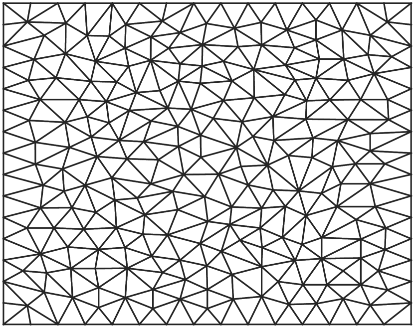
Figure 2: Example unstructured 2D mesh for convection-diffusion equation.

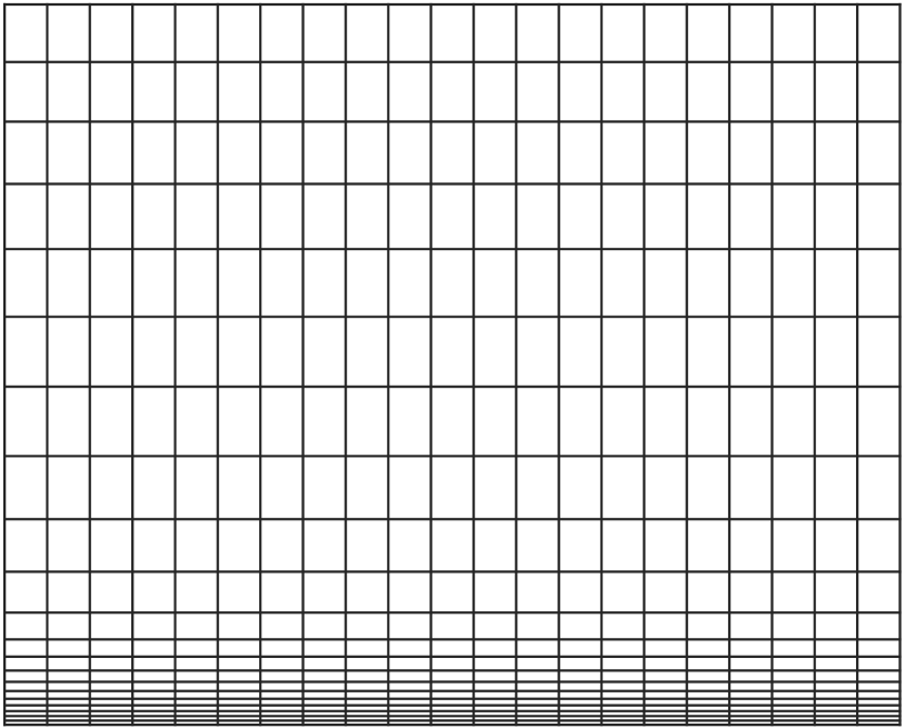
Figure 3: Example nonuniform structured mesh for Helmholtz equation.

E2CDb is based on Example 6.1.2 in [23]. The domain is $\Omega=[-1,1]^{2}$, with $\mu=1/200$ and $f=0$. The wind velocity is $\boldsymbol{\nu}=\left[0,1+(x+1)^{2}/4\right]^{T}$, which is vertical but increases in strength from left to right. Natural boundary conditions are applied on the top wall. Dirichlet boundary conditions are imposed elsewhere, with $u=1$ on the lower wall, and $u$ decreases cubically and quadratically to zero on the left and right walls, respectively. E2CDc is similar to E2CDb, except for a smaller diffusion coefficient $\mu=1/2000$. E2CDd and E2CDe are based on Example 6.1.4 in [23], known as the recirculating wind problem or double-glazing problem, which models the temperature distribution in a cavity $\Omega=[-1,1]^{2}$ heated by an external wall. The source term is $f=0$, and the wind velocity is $\boldsymbol{\nu}=\left[2y(1-x^{2}),-2x(1-y^{2})\right]$, which determines a recirculating flow. Dirichlet boundary conditions are imposed with $u=1$ on the right wall and $u=0$ elsewhere. For E2CDd and E2CDe, $\mu$ is $1/200$ and $1/2000$, respectively.

E3CDb-c solve the equation on $\Omega=[-1,1]^{3}$, with Dirichlet boundary conditions

$$u(\boldsymbol{x})=\begin{cases}1,&0\leq x,y\leq 0.5\text{ and }z=0,\\ 0,&\text{otherwise}.\end{cases}$$

The source term is $f=0$, and the wind velocity is $\boldsymbol{\nu}=\left[1-z,1-z,1\right]$. For E3CDb and E3CDc1-2, the dynamic viscosity is $\mu=10^{-12}$ and $10^{-6}$, respectively. These problems are convection dominant, and the FEM solutions may suffer from spurious oscillations on coarse meshes. Hence, these problems may not be relevant physically but are challenging algebraically.

Convection-Diffusion Equation with GFDM and AES-FEM.

GD$d$CD, for $d=2$ and $3$, were generated using our in-house implementation of GFDM. Similarly, AE$d$CD were generated using our in-house implementation of AES-FEM. The boundary conditions and parameters are the same as E$d$CDa.

Convection-Diffusion Equation with DG.

DG2CD solves the convection-diffusion equation using discontinuous Galerkin (DG). We implemented it in FEniCS. The domain is $\Omega=[0,1]^{2}$, with Dirichlet boundary conditions $u=\sin(5\pi y)$ on all sides. The dynamic viscosity is $\mu=2$, the wind velocity is $\boldsymbol{\nu}=[x-0.5,0]$, and the source term is $f=3$.

Helmholtz Equation with FDM.

D2HMa-c solve the Helmholtz equations using FDM on curvilinear meshes, contributed by our collaborator Dr. Marat Khairoutdinov, who is a climate scientist, and our colleague Oliver Yang. These equations arise from a 3D Poisson equation for pressure $p$ in the longitude-latitude coordinate system in a global climate model,

$$\frac{\partial^{2}p}{\partial x^{2}}+\mu(y)\frac{\partial}{\partial y}\left(\mu(y)\frac{\partial p}{\partial y}\right)+\frac{\mu(y)^{2}}{\rho(z)}\frac{\partial}{\partial z}\left(\rho(z)\frac{\partial p}{\partial z}\right)=\mu(y)^{2}f,$$ (36)

with natural boundary conditions. By applying Fourier transform along in $x$-direction to the 3D system, we obtain a collection of 2D Helmholtz equations in the frequency domain,

$$\mu\left(y\right)\frac{\partial}{\partial y}\left[\mu\left(y\right)\frac{\partial p}{\partial y}\right]+\frac{\mu\left(y\right){}^{2}}{\rho\left(z\right)}\frac{\partial}{\partial z}\left[\rho\left(z\right)\frac{\partial p}{\partial z}\right]-\omega^{2}p=\tilde{f},$$ (37)

where $\omega$ corresponds to the frequency. This equation is then discretized using conservative, cell-centered finite differences. The mesh in the $z$-direction is highly anisotropic, as illustrated in Figure 3 at a much coarser resolution. The frequency $\omega$ is zero for one of the $yz$-planes, and in this case the system is singular, which is a challenging problem in its own right and is beyond the scope of this study. For the adjacent planes, $\omega$ can be arbitrarily close to zero, depending on the grid resolution along $x$. D2HMa-c correspond to $\omega^{2}=10^{-13}$, $10^{-10}$, and $10^{-6}$, respectively. The strong anisotropy makes these Helmholtz equations difficult, especially for small $\omega$.

Incompressible Navier-Stokes Equations with FEM.

E$d$INS* solve the incompressible Navier-Stokes equations, which read

$$\rho(\dot{\boldsymbol{u}}+\boldsymbol{u}\cdot\boldsymbol{\nabla}\boldsymbol{u})-\boldsymbol{\nabla}\cdot\boldsymbol{\sigma}(\boldsymbol{u},p)= \boldsymbol{f},$$ (38)

$$\boldsymbol{\nabla}\cdot\boldsymbol{u}= 0,$$ (39)

where $\rho$ denotes density, $\boldsymbol{u}$ the fluid velocity, $\dot{\boldsymbol{u}}$ the acceleration, $\boldsymbol{\sigma}$ the stress tensor, and $\boldsymbol{f}$ an applied body force. For a Newtonian fluid,

$$\boldsymbol{\sigma}(\boldsymbol{u},p)=2\mu\boldsymbol{\epsilon}(\boldsymbol{u})-p\boldsymbol{I},$$ (40)

where $\mu$ is the dynamic viscosity and $\boldsymbol{\epsilon}(\boldsymbol{u})$ is the strain-rate-tensor

$$\boldsymbol{\epsilon}(\boldsymbol{u})=\frac{1}{2}\left(\boldsymbol{\nabla}\boldsymbol{u}+\left(\boldsymbol{\nabla}\boldsymbol{u}\right)^{T}\right).$$ (41)

Eqs. (38) and (39) are referred to as momentum and continuity equations, respectively. For the finite element methods, these equations are typically solved using Chroin’s method (see e.g. [46]), a.k.a. the projection method [14], which first solves the momentum equation and then solves Poisson equations to recover the divergence-free property. We discretize these equations using finite elements with FEniCS. We use the linear system from the first step, which is nonsymmetric. We obtain the right-hand side vectors after running the simulation for a few time steps, so that the flows are better developed and the vectors are more representative.

E2INSa1 and E2INSa2 correspond to the channel-flow problem over $\Omega=[0,1]^{2}$, with $\rho=1$ and $\mu=1$. We use Dirichlet boundary conditions $p=8$ and $p=0$ on the left and right walls, and $\boldsymbol{u}=\boldsymbol{0}$ on the top and bottom walls. E3NS is a similar problem in 3D, with natural boundary conditions along the $z$-direction. E2INSb and E2INSc correspond to a flow around a cylinder, which is a classical benchmark problem [53]. For E2INSb, $\nu=0.001=\mu/\rho$, with a corresponding to Reynolds number of $100$; for E2INSc, $\nu=0.0005$, with a corresponding Reynolds number of $200$. The remainder of the parameters were the same as those in [53]. E2INSb-c are very well-conditioned, with condition numbers less than $10^{3}$, so they represent the easiest problems in this benchmark set.

Compressible Navier-Stokes Equations with FVM.

V3CNS solves the compressible Navier-Stokes equations, which is a system of PDEs based on the conservation of mass, momentum, and energy. We use the matrix RM07R in Group Fluorem from the UF Sparse Matrix Collection, which solves the equation using the finite-volume methods (FVM); see [42] for more detail of the case. This problem is the most ill-conditioned in this benchmark set.

Stokes Equations with Mixed FEM.

E3STHa1 and E3STHa2 solve the Stokes equations, which describe a steady, incompressible Newtonian flow with low Reynolds numbers. For a domain $\Omega\subset\mathbb{R}^{d}$, the Stokes equations read

$$-\boldsymbol{\nabla}\cdot(\mu\boldsymbol{\nabla}\boldsymbol{u})+\boldsymbol{\nabla}p =\boldsymbol{f},$$ (42)

$$\boldsymbol{\nabla}\cdot\boldsymbol{u} =0,$$ (43)

where $\boldsymbol{u}$ denotes the fluid velocity, $\mu$ the dynamic viscosity, $p$ the pressure, and $\boldsymbol{f}$ an applied body force. This problem is unstable with linear elements. We solve it using mixed Taylor-Hood elements [24], which use quadratic elements for $\boldsymbol{u}$ and linear elements for $p$. The domain is a unit cube $\Omega=[0,1]^{3}$, with $\mu=2$ and $\boldsymbol{f}=\boldsymbol{0}$. The boundary condition is $\boldsymbol{u}=\left[-\sin(\pi y),0,0\right]$ for $x=1$ and $\boldsymbol{u}=\boldsymbol{0}$ everywhere else. The resulting linear system may be either symmetric and indefinite or nonsymmetric and positive definite; we used the nonsymmetric variant. A notable property of the linear system is that there is a large zero diagonal block, similar to saddle-point problems. We refer to these systems as saddle-point-like problems.

Poisson Equation with Mixed FEM.

E3MP is another example of saddle-point-like problems, from the mixed formulation of the Poisson equation $-\Delta u=f$. This formulation introduces a vector field, namely $\boldsymbol{v}=\boldsymbol{\nabla}u$, and then constructs a system of first-order PDEs

$$\boldsymbol{v}-\boldsymbol{\nabla}u =\boldsymbol{0}\qquad\,\,\,\,\text{ in }\Omega,$$ (44)

$$\boldsymbol{\nabla}\cdot\boldsymbol{v} =-f\qquad\text{ in }\Omega.$$ (45)

See e.g. [10] for details on mixed FEM. These equations are similar to those arising from the Darcy flow in porous media. We solve the equations using FEniCS with linear Brezzi-Douglas-Marini elements for $u$ and degree-$0$ discontinuous elements for $\boldsymbol{v}$. The domain is $\Omega=[0,1]^{3}$, with homogeneous Dirichlet boundary conditions along the left and right walls, and Neumann boundary conditions $\boldsymbol{v}\cdot\boldsymbol{n}=\sin(5x)$ elsewhere. The source term was $f=10\exp(-((x-0.5)^{2}+(y-0.5)^{2}+(z-0.5)^{2})/0.02)$.

5 Numerical Comparisons

In this section, we present numerical comparisons of the preconditioned Krylov methods described in Sections 3. For GMRES, TFQMR, and BiCGSTAB, we use the built-in implementations in PETSc v3.7.1. For GMRES, we use 30 as the restart parameter, which is the recommended value for large-scale linear systems in PETSc, and we denote the method by GMRES(30). For QMRCGSTAB, which is unavailable in PETSc, we use our implementations based on the low-level functions in PETSc. In terms of preconditioners, we consider Gauss-Seidel (GS), ILU0, ILUTP (SuperLU v5.2.1), MILU (ILUPACK v2.4), variants of classical AMG (BoomerAMG in hypre v2.11.0), and smoothed-aggregation AMG (Trilinos/ML 5.0), all as right preconditioners. For a uniform comparison, we set the relative convergence tolerance for the $2$-norm of the residual, i.e., the 2-norm of the residual divided by the 2-norm of the right-hand side, to $10^{-10}$ for all methods.

As an overview, Table 4 shows the runtimes of all the benchmark problems described in Section 4 with GMRES(30), which is the most robust. All the tests were conducted in serial on a single node of a cluster with two 2.6 GHz Intel Xeon E5-2690v3 processors and 128 GB of memory. For accurate timing, both turbo and power saving modes were turned off for the processors, and each node was dedicated to run one problem at a time. In the table, the best timing results were in bold, ‘-’ indicates stagnation, ‘*’ indicates “did not converge” after 10,000 iterations, and ‘$\times$’ indicates runtime errors in SuperLU (in particular, nontermination of factorization after 24 hours for E3STHa2 and malloc errors for the others). For ILUTP, we used SuperLU with the default drop tolerance of $10^{-4}$. For hypre/BoomerAMG, we used HMIS coarsening with FF1 interpolation for all cases except for E2CDc, which used PMIS+FF1 due to non-convergence with HMIS+FF1. The other parameters are all default. It is clear that hypre is the overall winner for convection-diffusion and Helmholtz equations. However, Gauss-Seidel is the most efficient for well-conditioned systems, such as those from incompressible Navier-Stokes equations. We will not consider the well-conditioned systems further. On the other end, multilevel ILU tends to be the most robust for ill-conditioned and saddle-point-like problems. In the following subsections, we give more detailed comparisons in terms of convergence of different KSP methods, ILU, and multigrid preconditioners.

Table 4: Overview of runtimes (in seconds) of GMRES(30) with Gauss-Seidel, ILU0, ILUTP, MILU, hypre, and ML. ‘$-$’, ‘*’, and ‘$\times$’ indicate stagnation, “did not converge,” and runtime error, respectively.

Matrix ID	GS	ILU0	ILUTP	MILU	HYPRE	ML
E2CDa	1,517.3	1,390.5	85.3	143.0	7.52	17.88
E2CDb	5,554.2	2,527.4	917.9	1,173.6	38.14	246.7
E2CDc	3,355.2	1,377.8	574.2	1,107.2	71.1*	236.3
E2CDd	*	*	881.4	1,309.6	44.41	747.8
E2CDe	*	*	2,287.1	1,291.5	77.10	2,936.1
E3CDa1	20.41	12.63	1,158.4	17.35	5.75	8.48
E3CDa2	263.8	157.9	32,389.5	179.3	51.40	70.05
E3CDa3	7,191.2	5,126.1	$\times$	2,430.1	572.93	853.4
E3CDb	366.4	213.6	55,372.5	1,314.3	52.28	84.17
E3CDc1	292.13	172.04	54,793.1	1,313.1	55.0	77.05
E3CDc2	2,744.4	1,548.7	$\times$	2,125.7	232.9	360.60
AE2CD	416.5	280.5	128.9	59.2	18.2	25.3
AE3CD	6140.3	5018.5	$\times$	2,440.9	534.3	819.1
GD2CD	1,543.1	1,230.5	87.01	142.65	8.45	23.49
GD3CD	178.40	113.7	42,819.9	168.1	50.79	69.66
DG2CD	*	*	180.79	145.4	10.60	21.49
D2HMa	*	*	223.5	131.2	5.42	211.7
D2HMb	*	*	30.67	78.1	5.96	35.93
D2HMc	1.11	0.91	18.36	9.6	0.91	7.40
E2INSa1	846.2	778.9	273.34	171.2	938.8	1020.7
E2INSa2	1,336.2	1,048.9	192.79	217.5	1,175.6	1861.3
E2INSb	58.8	78.16	$\times$	672.7	148.7	165.8
E2INSc	107.2	129.3	$\times$	426.8	339.1	232.9
E3INS	383.9	392.1	$\times$	617.4	785.5	732.1
V3CNS	*	*	*	21,039.6	*	*
Saddle-point-like problems
E3STHa1	$-$	$-$	86.7	7.74	$-$	$-$
E3STHa2	$-$	$-$	$\times$	375.5	$-$	$-$
E3MPa1	$-$	$-$	4,033.2	129.4	$-$	$-$
E3MPa2	$-$	$-$	43,385.4	352.6	$-$	$-$

5.1 Comparison of Krylov-Subspace Methods

We first compare the four different Krylov-subspace methods. We consider three preconditioners: GS (available as SOR with relaxation parameter $\omega=1$ in PETSc), ILU0 (the default serial preconditioner in PETSc), and BoomerAMG with HMIS coarsening and FF1 interpolation (which differs from the default option in hypre). In Sections 5.2 and 5.3, we will compare the different variants of ILU and AMG, respectively.

5.1.1 Convergence Comparison.

Theoretically, the asymptotic convergence of the Krylov subspace methods may be analyzed using the distributions of eigenvalues and (generalized) eigenvectors. In practice, however, the convergence is complicated by the restarts in Arnoldi iterations and the nonorthogonal basis in the bi-Lanczos iteration. To complement theoretical analysis, we present the convergence history of ten test cases in Figures 4–8, which are representative of the others. Note that we plot the relative residuals with respect to the numbers of matrix-vector products instead of iteration counts, because the former is a better indication of the overall computational cost and also of the degrees of the polynomials. For ease of cross-comparison of different preconditioners, we truncated the $x$-axis to be the same for Gauss-Seidel and ILU0 for each matrix.

Figure 4 shows the convergence history of test cases E2CDa and E3CDa3. With Gauss-Seidel or ILU0 preconditioners, GMRES converged fast initially but then slowed down drastically due to restart, whereas BiCGSTAB had highly oscillatory residuals because its formulation does not minimize the residual in any norm or pseudo-norm. QMRCGSTAB was much smoother than BiCGSTAB, and it sometimes converged faster than BiCGSTAB. The convergence of TFQMR exhibited a staircase pattern, indicating frequent near stagnations due to its sensitivity to rounding errors. With BoomerAMG, however, the four methods had about the same convergence trajectories. GMRES converged slightly faster than the others, but all the methods converged quite smoothly, without any apparent oscillation or stagnation. These results indicate that an effective multigrid preconditioner can potentially overcome the disadvantages of each of these KSP methods, including slow convergence with restated GMRES, oscillations with BiCGSTAB, and near stagnation with TFQMR. Figure 5 shows the convergence results for GD2CD and GD3CD. The results are qualitatively similar to those of E2CDa and E3CDa3, except that the near stagnation of TFQMR is even more apparent.

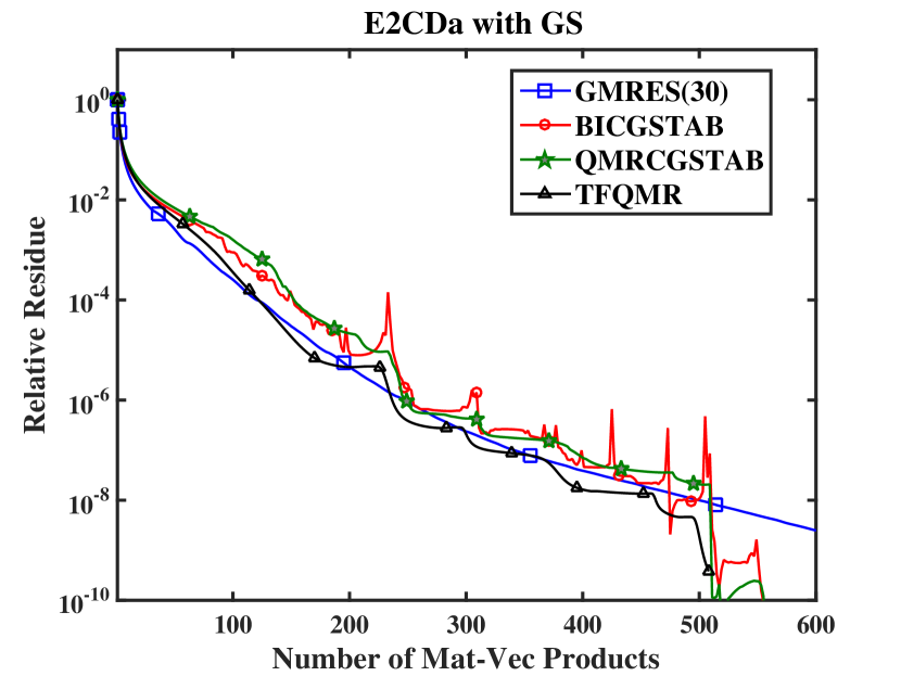
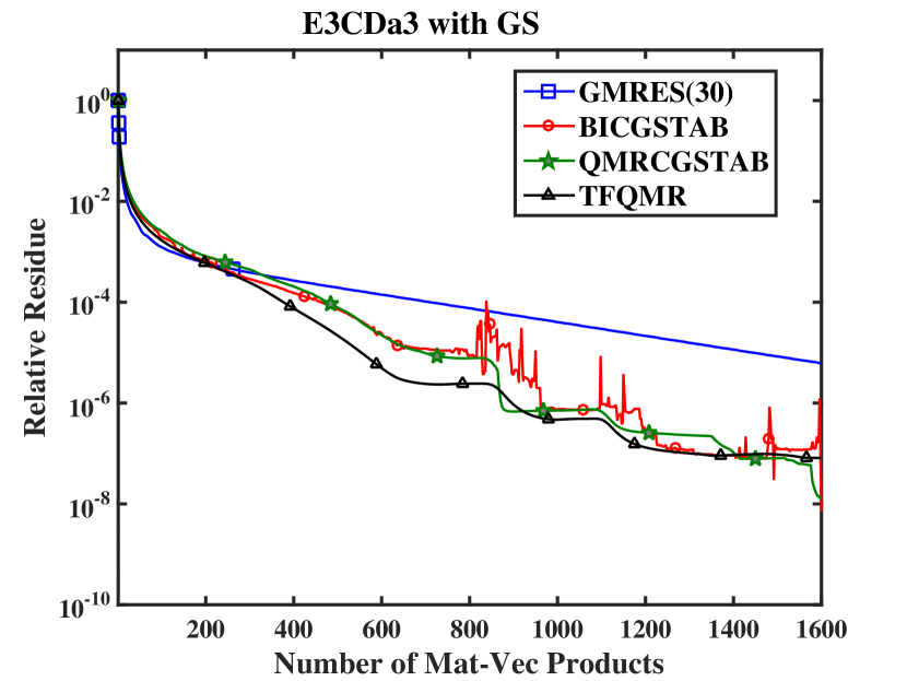
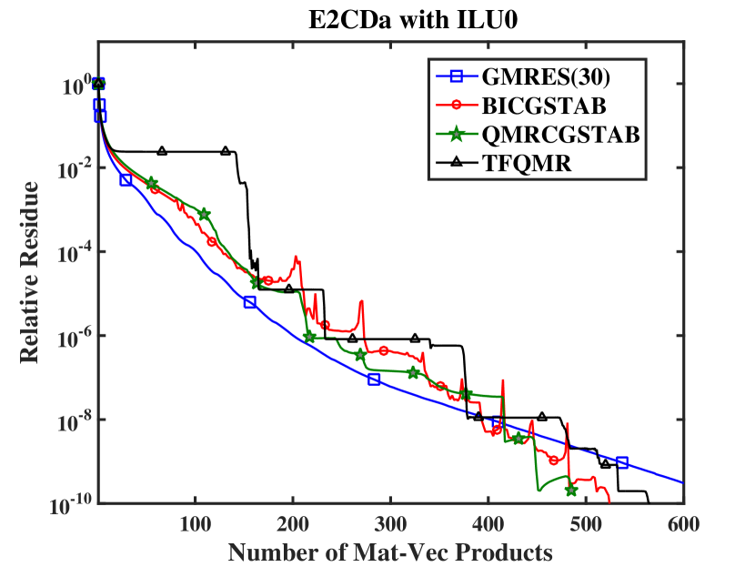
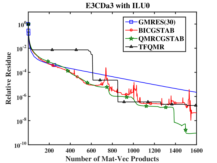
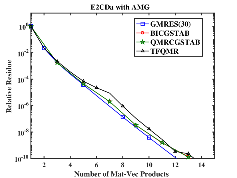
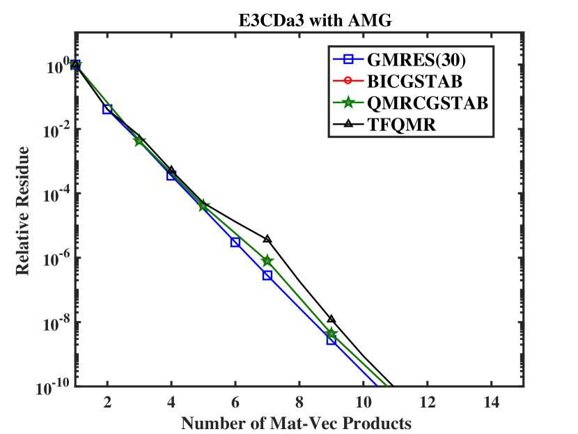
Figure 4: Residuals vs. numbers of matrix-vector products for E2CDa (left) and E3CDa3 (right).

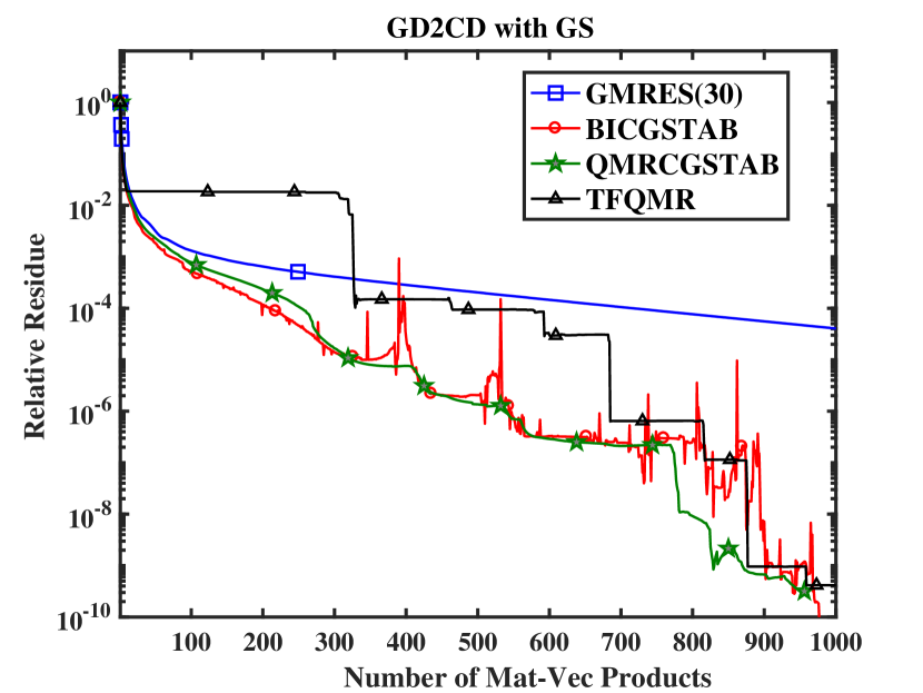
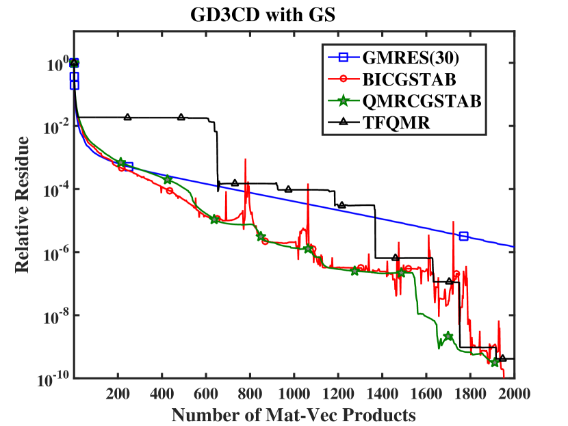
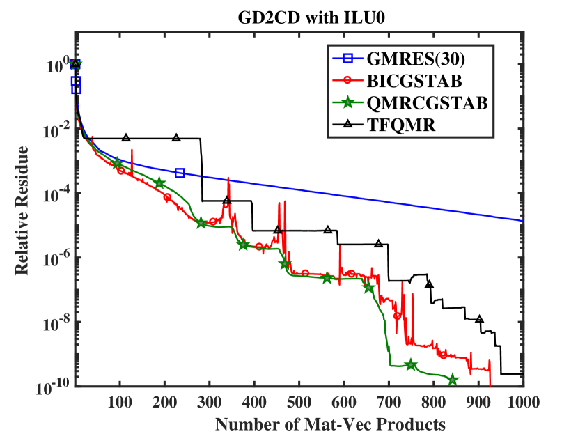
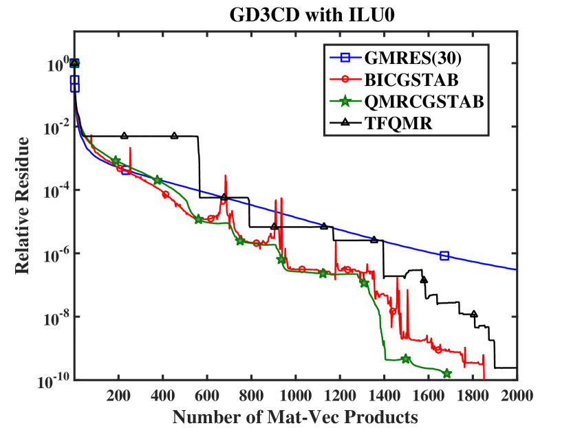
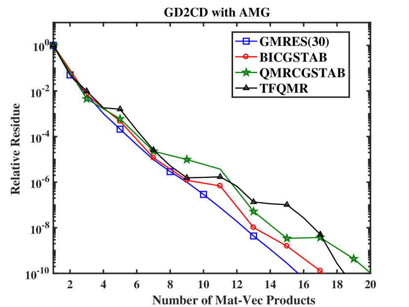
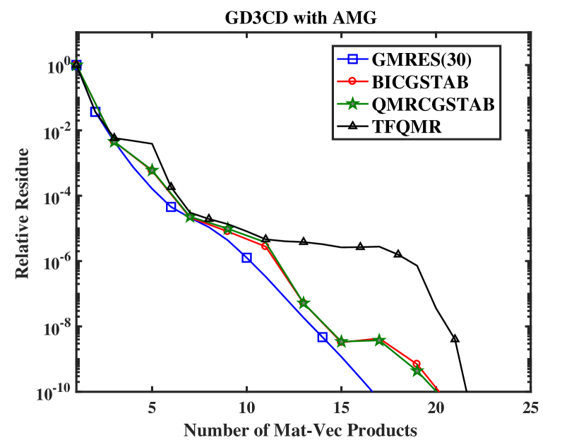
Figure 5: Residuals vs. numbers of matrix-vector products for GD2CD (left) and GD3CD (right).

Figure 6 shows the convergence results for E2CDb and E3CDb. The most notable new feature is that for E2CDb, BiCGSTAB diverged with Gauss-Seidel and ILU0. QMRCGSTAB with Gauss-Seidel converged, so did GMRES with ILU0, but all other methods with Gauss-Seidel and ILU0 stagnated. For E3CDb, all the methods converged with Gauss-Seidel and ILU0. Although BiCGSTAB converged relatively smoothly, the residuals had notable jumps near the end. TFQMR had a plateau even with AMG, again due to its sensitivity to round-off errors. Note that QMRCGSTAB overcame the oscillations with BiCGSTAB and the near stagnations with TFQMR, and it converged the fastest in some cases.

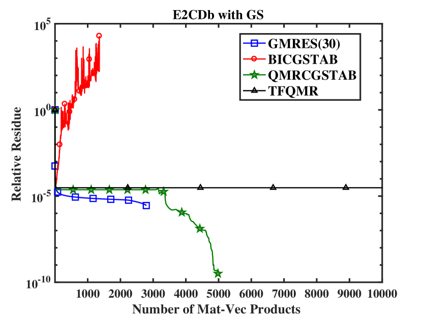
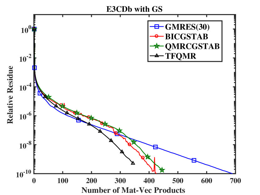
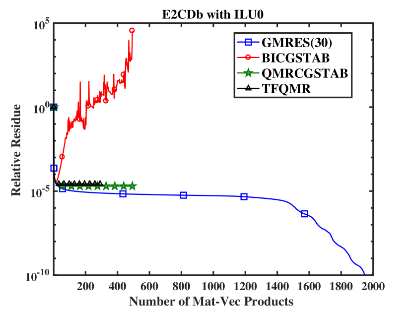
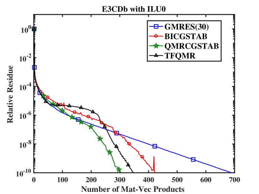
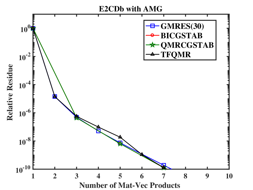
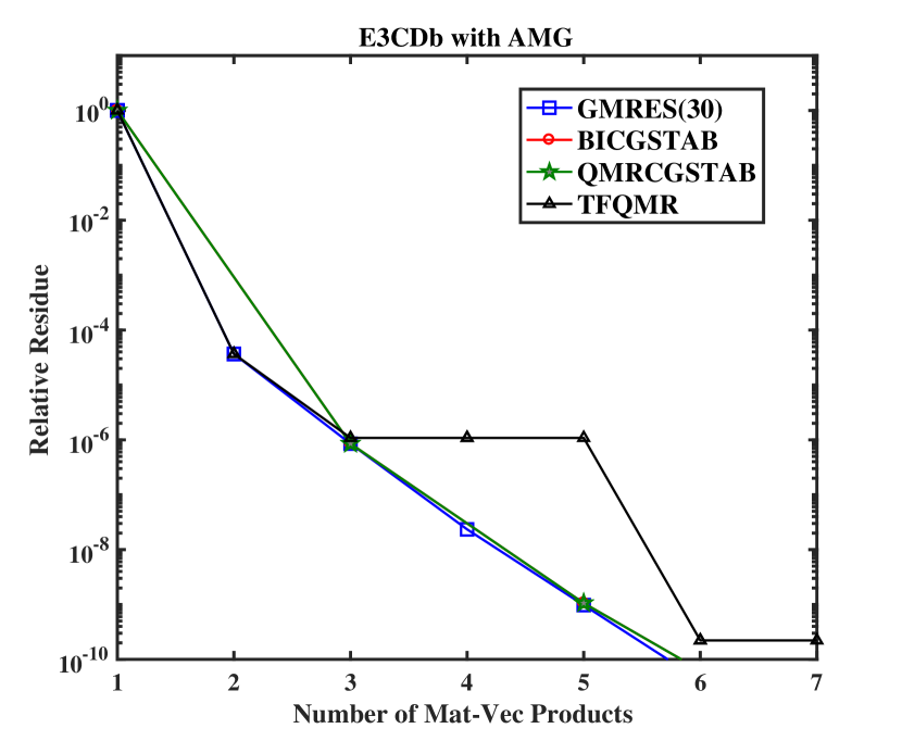
Figure 6: Residuals vs. numbers of matrix-vector products for E2CDb (left) and E3CDb (right).

Figure 7 shows the convergence results for DG2CD and D2HMa. The condition number of DG2CD is about $10^{7}$, and its results were qualitatively similar as GD2CD and GD3CD. The condition number of D2HMa is nearly $10^{9}$, and this ill-conditioning caused difficulties for virtually all the methods with GS and ILU0 preconditioners. GMRES and TFQMR both stagnated. BiCGSTAB oscillated wildly, while QMRCGSTAB had smoother trajectories. With BoomerAMG, all the methods converged rapidly and smoothly, while GMRES converged slightly faster than the others.

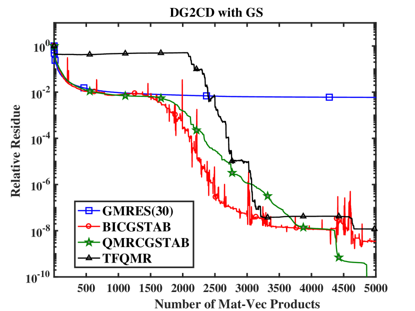
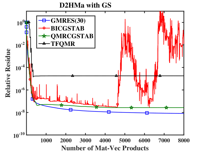
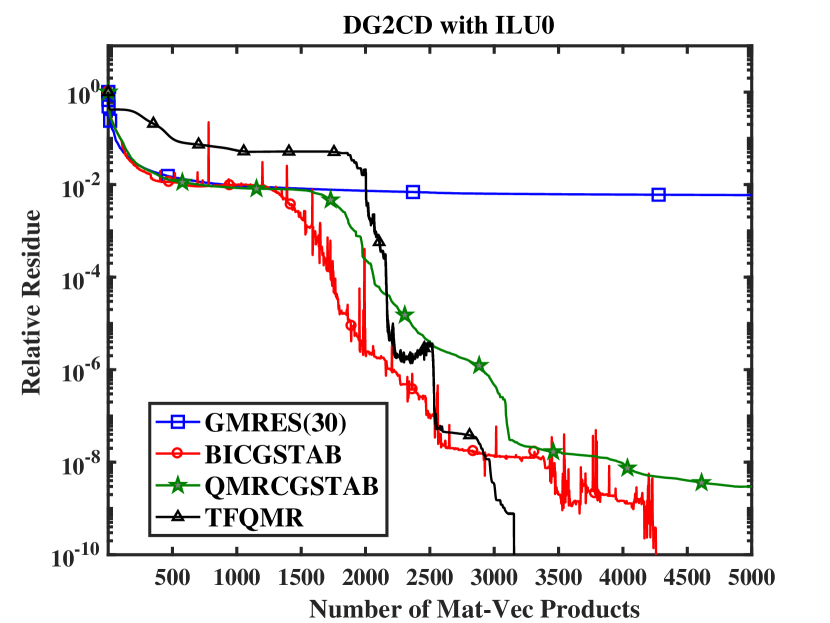
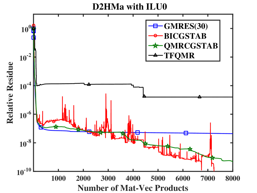
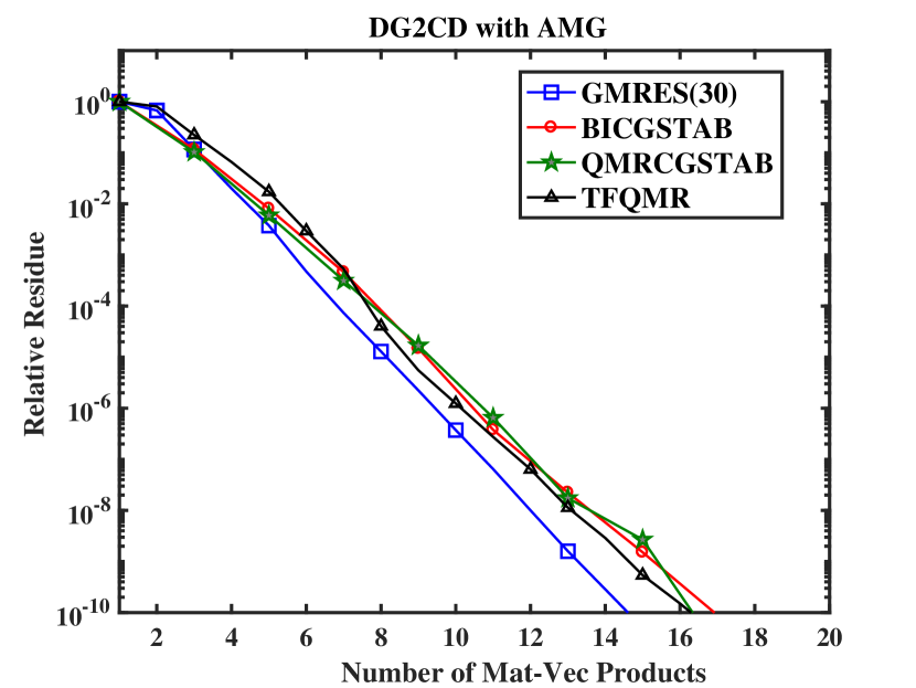
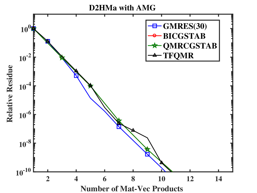
Figure 7: Residuals vs. numbers of matrix-vector products for DG2CD (left) and D2HMa (right).

Figure 8 shows the convergence results for E2INSa1 and E3INS. For E2INSa1, TFQMR stagnated with all the preconditioners. The other solvers delivered similar performance to each other. GMRES performed the best for E3INS. However, QMRCGSTAB and BiCGSTAB outperformed GMRES for E2INSa1, which required many iterations even with AMG.

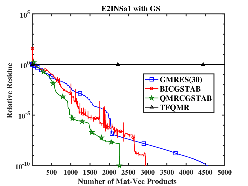
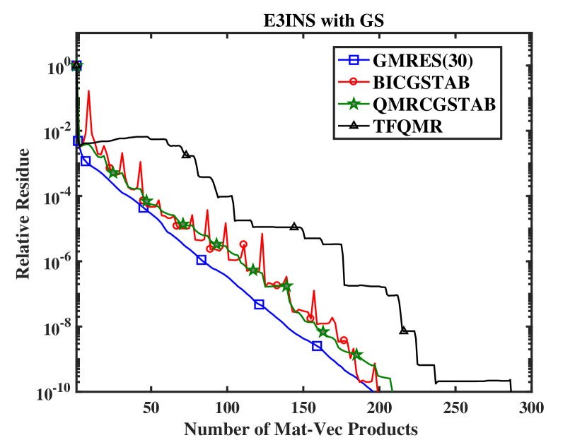
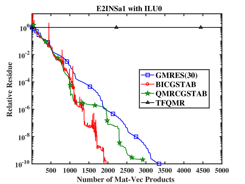
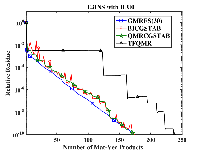
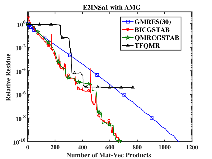
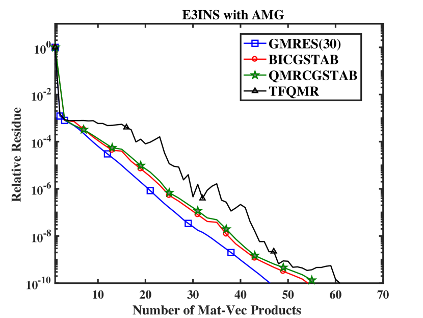
Figure 8: Residuals vs. numbers of matrix-vector products for E2INSa1 (left) and E3INS (right).

From these results, we make the following observations. If relatively few iterations are needed to converge, especially with an effective multigrid preconditioner, GMRES converges the fastest, because it minimizes the 2-norm of the residual. However, if many iterations are needed, then the advantage of GMRES diminishes, and a method with a three-term recurrence can be more reliable. BiCGSTAB and TFQMR suffer from oscillatory residuals and frequent plateaus, respectively. By design, QMRCGSTAB overcomes both of these shortcomings [15].

5.1.2 Timing Comparison.

The convergence histories are helpful in revealing the intrinsic properties of the KSP methods, but in practice the overall runtime is the ultimate criterion. Figure 9 compares the runtimes of seven cases from those in Section 5.1.1 along with AE3CD. We circled out the best performances for each case. It can be seen that for six out of eight cases, BoomerAMG accelerated KSP significantly better than Gauss-Seidel and ILU0. GMRES with BoomerAMG was the best in these cases, while BiCGSTAB and QMRCGSTAB were close runners-up. With GS and ILU0, GMRES was significantly slower than the others due to restarts. For Navier-Stokes equations, BiCGSTAB with Gauss-Seidel and ILU0 delivered better performance than AMG. QMRCGSTAB had similar performance as BiCGSTAB.

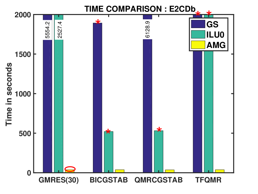
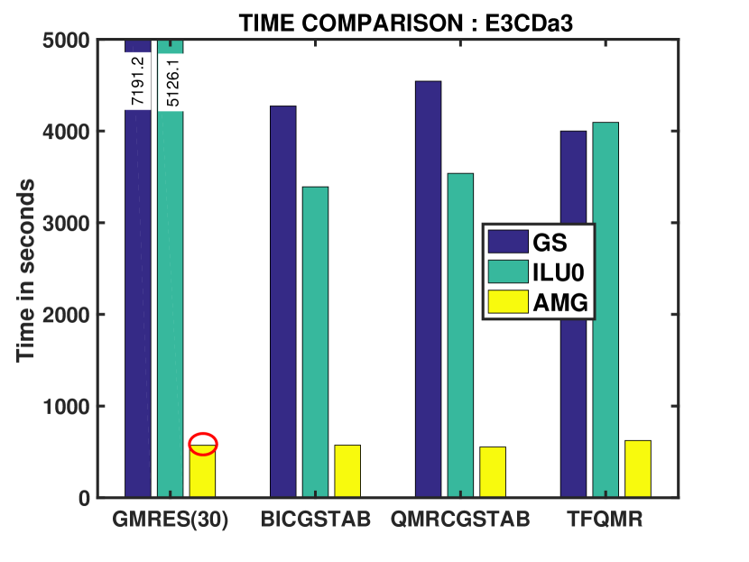
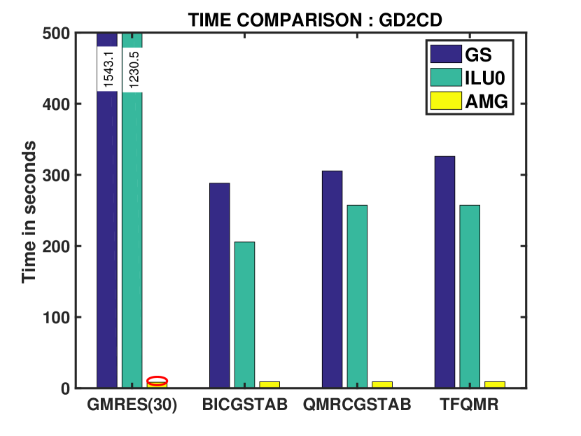
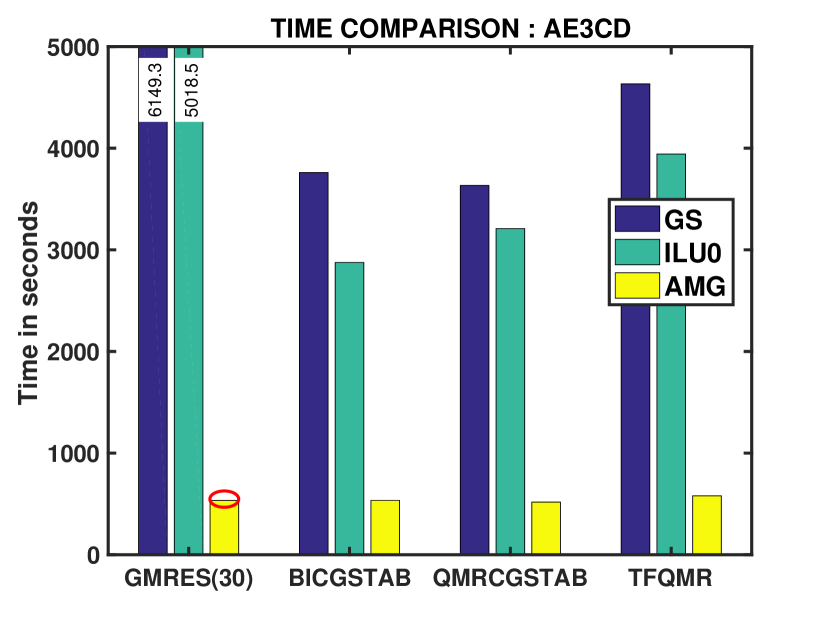
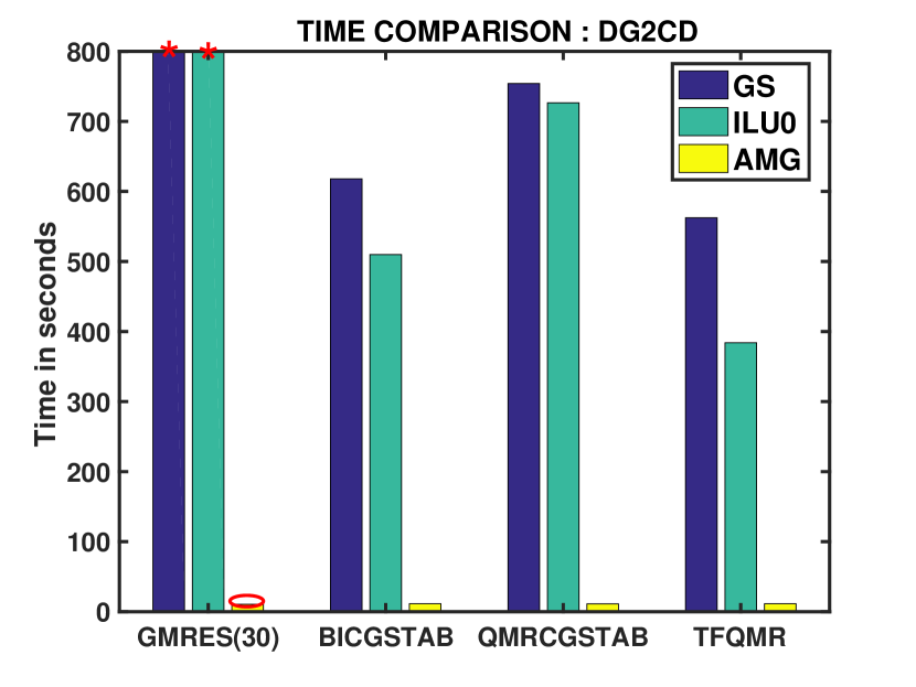
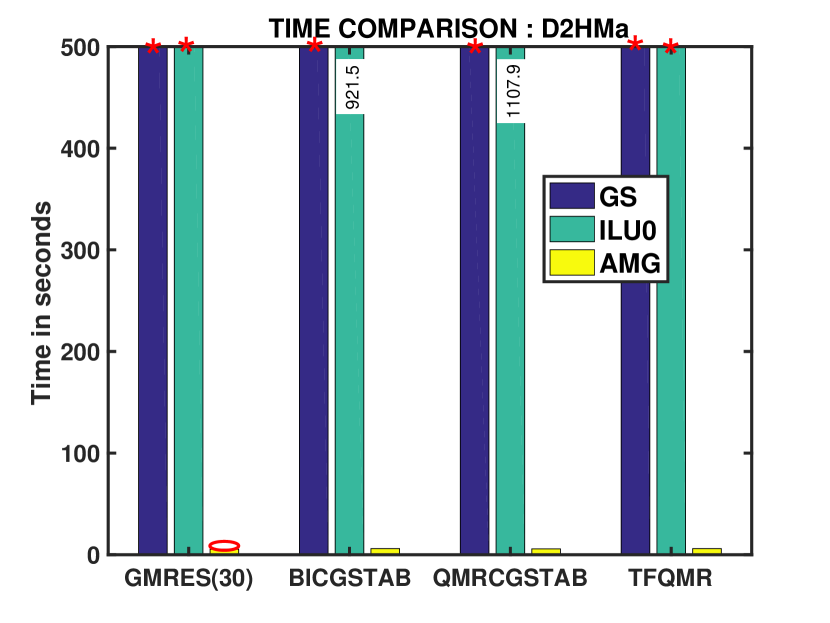
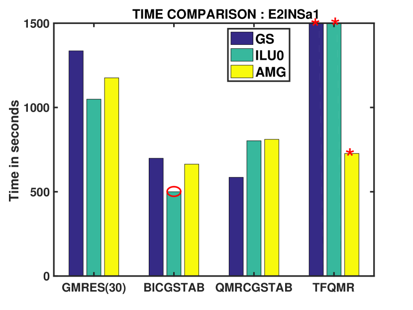
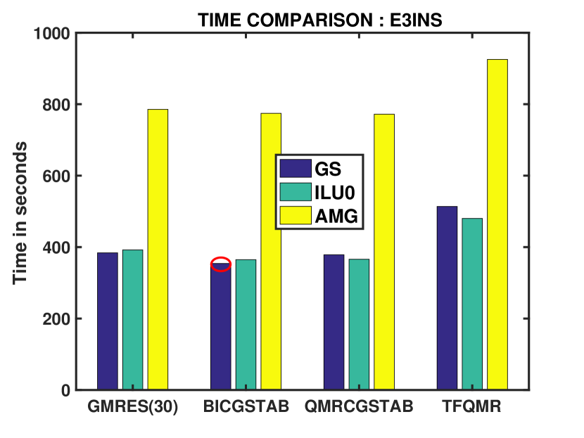
Figure 9: Comparison of timing results for eight representative cases. Circled bars indicate best results. ‘*’ indicates non-convergence or stagnation after 10,000 iterations.

Overall, the timing results are consistent with the convergence results, so the numbers of matrix-vector products are indeed good predictors of the overall performance. Among the bi-Lanczos-based methods, BiCGSTAB is slightly more efficient due to its lower cost per iteration, but QMRCGSTAB is a competitive alternative, especially if smooth convergence is desired. In addition, we observe that the continuum formulations of the PDEs, rather than the discretization methods, tend to have a bigger impact on the choice of preconditioners. In particular, AMG can significantly outperform Gauss-Seidel and ILU0 for convection-diffusion equations, independently of discretization methods, but AMG is not very effective for incompressible Navier-Stokes equations.

5.1.3 Asymptotic Growth with Respect to Problem Size.

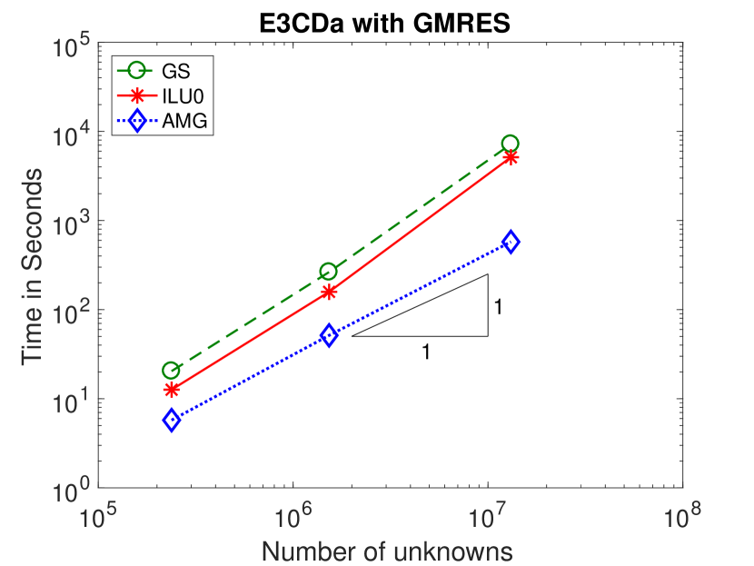
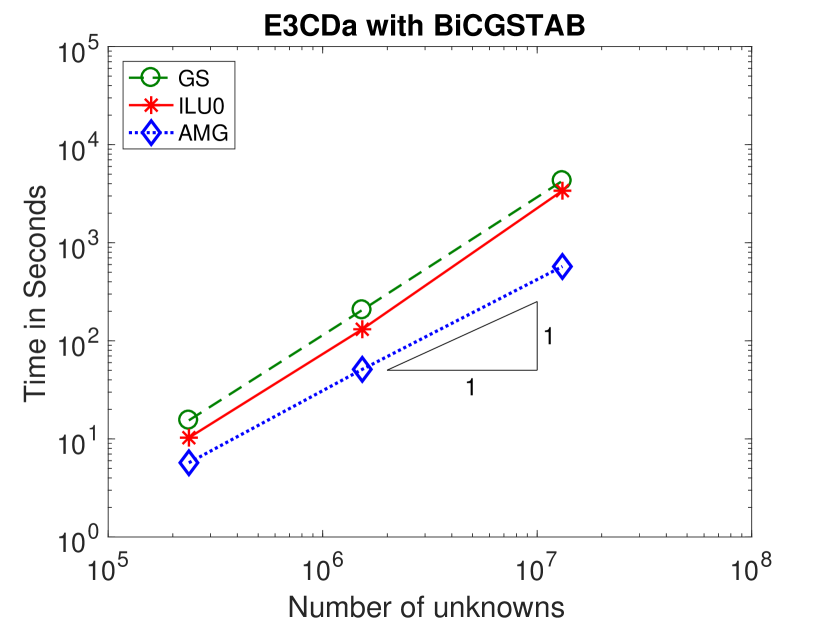
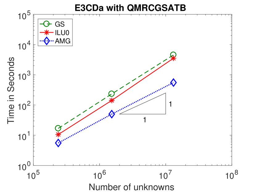
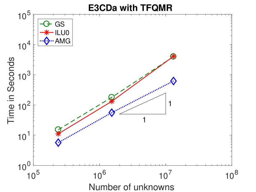
Figure 10: Asymptotic growth of runtimes of the preconditioned solvers for E3CDa1-3.

The relative performance of preconditioned KSP methods may depend on problem sizes, because different methods may scale differently with respect to the problem sizes. To assess the asymptotic complexity of the methods, we consider matrices E3CDa1-3, whose numbers of unknowns grow approximately by a factor of 8 between each adjacent pair. Figure 10 shows the timing results of the four Krylov subspace methods with Gauss-Seidel, ILU0, and BoomerAMG. The $x$-axis corresponds to the number of unknowns, and the $y$-axis corresponds to the runtimes, both in logarithmic scale. For a perfectly scalable method, the slope should be 1. We observe that with AMG, the slopes for the four KSP methods are all close to 1. The slopes for Gauss-Seidel and ILU0 were greater than 1, so the numbers of iterations would grow as the problem size increases. Therefore, the advantage of multigrid preconditioners is more significant for larger systems.

5.2 Comparison of Variants of ILU

We now compare the performance of GMRES with ILU0, ILUTP (in particular, the supernodal ILUTP implementation in SuperLU v5.2.1), and MILU (in particular, its implementation in ILUPACK v2.4). We first compare the scalabilities of their setup and solve times with respect to the number of unknowns in Figure 11 for E3CDa1-3. ILUTP failed for E3CDa3 due to malloc errors in SuperLU, and hence we only show their results for E3CDa1-2. For ILU0, the setup times grow linearly, but its solve time is higher than MILU with drop tolerance $10^{-1}$. For ILUTP, the setup times grow superlinearly with either the default drop tolerance $10^{-4}$ or a larger drop tolerance $10^{-3}$, making it orders of magnitude slower than MILU for larger problems. For MILU, both the setup and solve times grow nearly linearly.

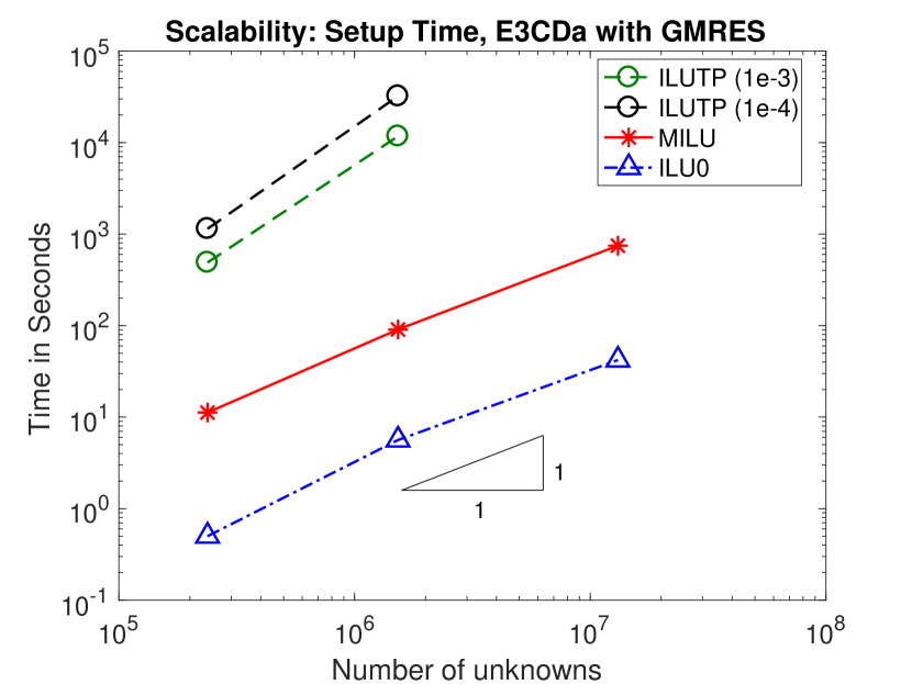
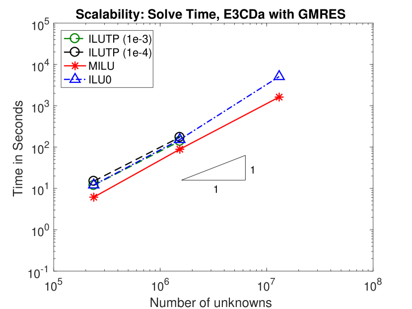
Figure 11: Asymptotic growth of setup (left) and solve times of ILU0 in PETSc, supernodal ILUTP in SuperLU with drop tolerance $10^{-4}$ (default) and $10^{-3}$, and MILU in ILUPACK for E3CDa1-3.

To compare the overall performance of the methods, Figure 13 compares the runtimes of the three preconditioners for six representative cases. For ILUTP, we used the drop tolerance $10^{-3}$; for MILU, we used the default parameters. For E3CDa3 and E3NS, ‘*’ indicates failure of ILUTP due to malloc error in SuperLU; for D2HMa, ‘*’ indicates GMRES with ILU0 did not converge after 10,000 iterations. ILU0 was the best in two out of six cases, due to its low setup cost. However, it significantly underperformed in the other four cases. Between MILU and ILUTP, MILU outperformed for all the cases. Note that in [37], the opposite conclusion was drawn, where the test cases had thousands, instead of millions, of unknowns. However, we note that even though MILU worked well for D2HMa and E3CDa1, it still underperformed BoomerAMG by nearly two orders of magnitude for these cases.

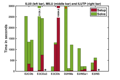
Figure 12: Comparison of runtimes of GMRES with ILU0, MILU, and ILUTP.

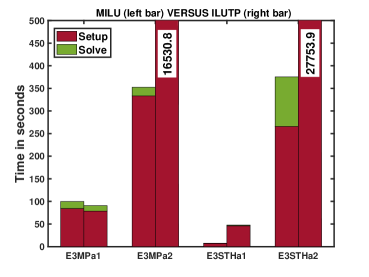
Figure 13: Comparison of runtimes of MILU vs. ILUTP for saddle-point-like problems.

The main advantage of MILU, and also of ILUTP to some extent, is that they are much more robust for ill-conditioned and saddle-point-like problems. As shown in Table 4, MILU was the only preconditioner that enabled GMRES to solve V3CNS. This highlights the robustness of MILU for ill-conditioned systems. For saddle-point-like problems, only MILU allowed GMRES to solve the problems in a reasonable amount of time, although GMRES with ILUTP also converged. Figure 13 compares the setup times and runtimes of GMRES with MILU and ILUTP for the four saddle-point-like problems. For three out of four problems, MILU significantly outperformed ILUTP. Hence, MILU is the most robust choice for saddle-point-like problems.

5.3 BoomerAMG Versus ML

Finally, we compare two AMG preconditioners: BoomerAMG and ML, which are variants of classical AMG and smoothed aggregation, respectively. Both of these methods scale nearly linearly in terms of the number of unknowns. However, their actual performance may differ drastically. Figure 14 and 15 compare the convergence and runtimes of GMRES and BiCGSTAB with BoomerAMG and ML for seven representative results. We used HMIS coarsening with FF1 interpolation for BoomerAMG and the default parameters for ML. For six out of seven cases, BoomerAMG outperformed ML. The only case that ML outperformed BoomerAMG was E3INS, for which Gauss-Seidel also outperforms ML. For D2HMa, which is ill-conditioned, BoomerAMG was more than 20 times faster than ML. This is probably because for smoothed aggregation, too many aggregates can lead to the growth of complexity and irregularly shaped aggregates, which can cause poor convergence [66]. We note that we have tried many different options in ML, and the results were qualitatively the same.

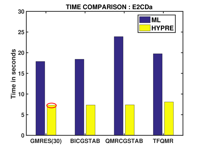
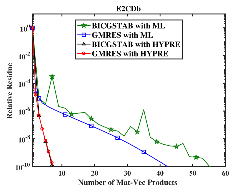
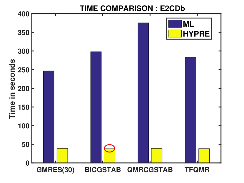
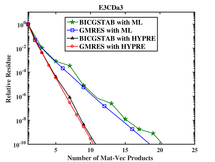
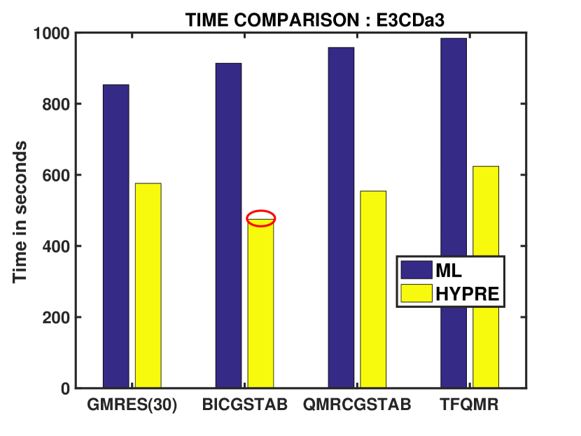
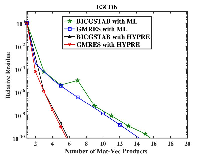
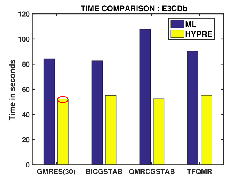
Figure 14: Convergence history (left) and runtimes (right) of GMRES and BiCGSTAB with BoomerAMG and ML. Circled bars indicate best performance.

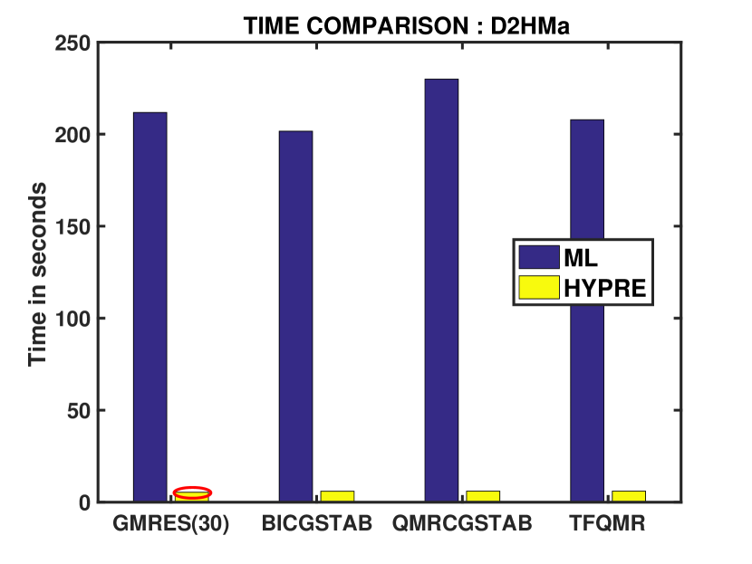
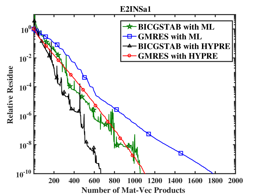
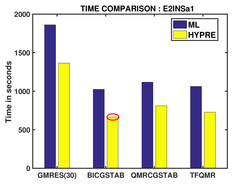
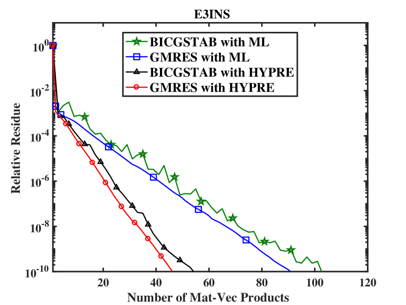
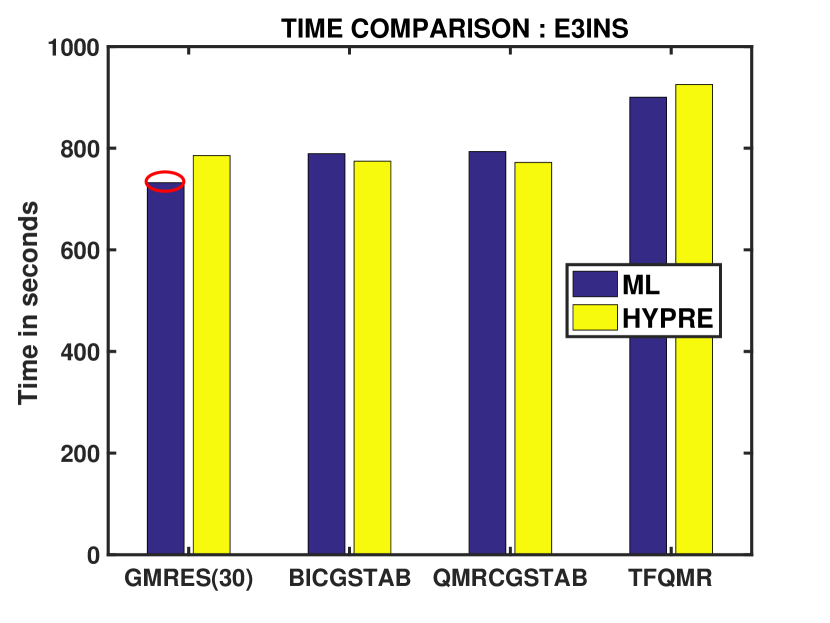
Figure 15: Convergence history (left) and runtimes (right) of GMRES and BiCGSTAB with BoomerAMG and ML. Circled bars indicate best performance.

In the above tests, BoomerAMG was clearly the winner. However, different coarsening and interpolation techniques in BoomerAMG may lead to drastically different performance, especially for 3D problems. Figure 16 presents a more in-depth comparison of the three coarsening strategies, namely Falgout, PMIS, and HMIS, along with ML. For Falgout coarsening, the “classical” interpolation is the most effective. For PMIS and HMIS, we consider both the extended+i interpolation and the modified FF interpolation (FF1). In all the cases, the interpolation matrices were truncated to 4 elements per row, as recommended by hypre manual [58]. We used the default values for the other parameters. It can be seen that the Falgout coarsening, delivered good performance in 2D, but it underperformed ML for 3D problems. However, PMIS+FF1 and HMIS+FF1 delivered significantly better performance than ML for 3D problems. Between PMIS+FF1 and HMIS+FF1, their performances were comparable, but HMIS outperformed PMIS for ill-conditioned problems. In addition, FF1 interpolation outperformed the extended+i interpolation for seven out of eight cases, probably because the truncation for extended+i is not very effective. Note that for E3INS, although ML outperformed HMIS+FF1, BoomerAMG with PMIS+FF1 still outperformed ML. Therefore, we consider BoomerAMG with HMIS+FF1 or PMIS+FF1 as the overall winner.

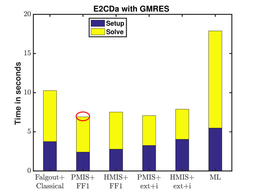
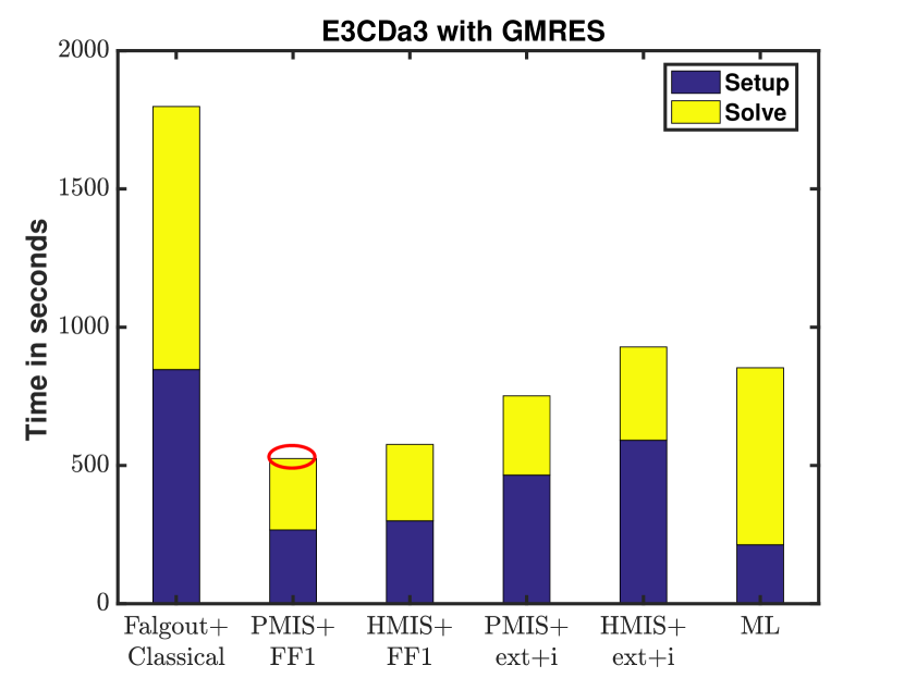
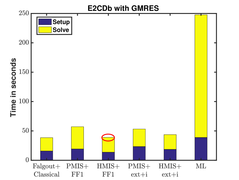
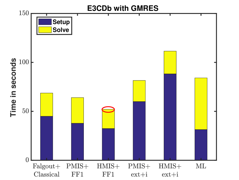
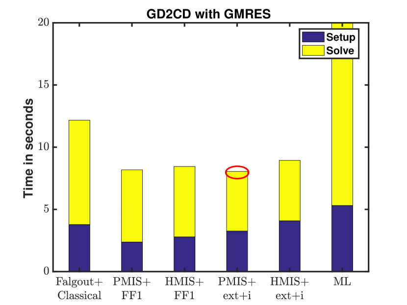
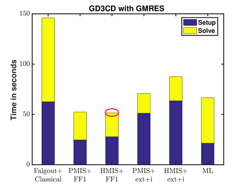
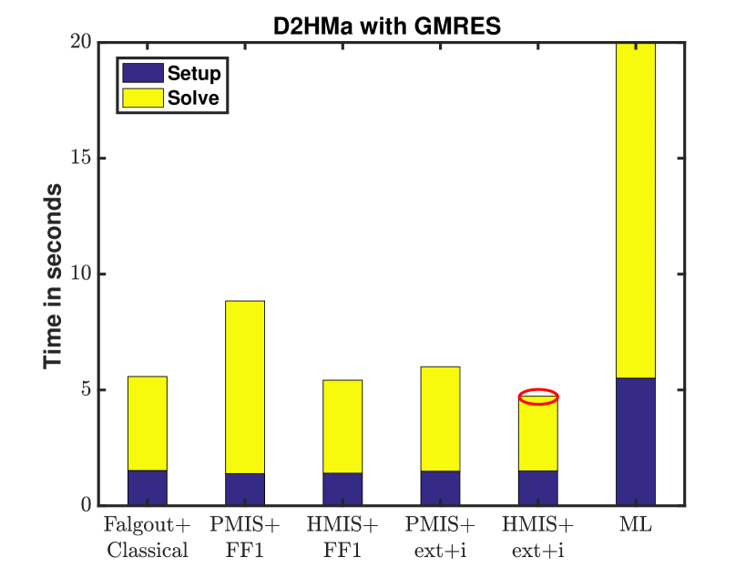
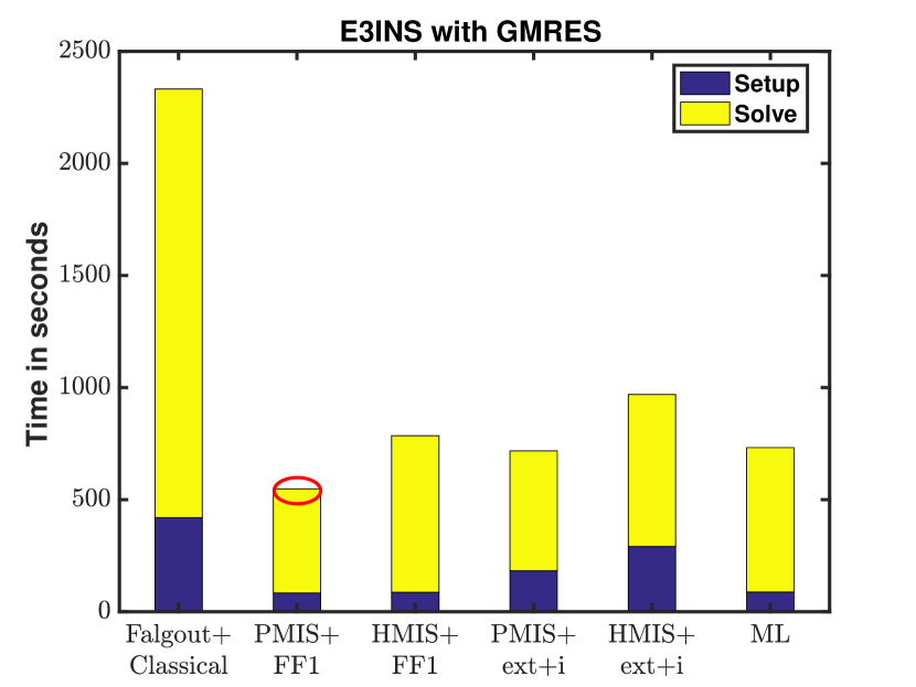
Figure 16: Comparisons of setup and solve times of BoomerAMG with five coarsening+interpolation strategies and ML. Circled bars indicate best performance.

We note that in the literature, it is sometimes reported that smoothed aggregation works better than classical AMG for 3D elasticity problems, which are generalizations of Poisson equations to vector-valued functions. We did not consider elasticity problems in this work, because their linear systems are symmetric; we refer readers to [4] for more discussions on AMG for elasticity. However, we comment that the aforementioned comparison for elasticity problems refers to the classical Ruge-Stüben coarsening, which, like Falgout coarsening in BoomerAMG, does not work well for 3D problems or for vector-valued PDEs. An advantage of smoothed aggregation is that it can naturally take into consideration the coupling of the variables in vector-valued PDEs. However, in Table 4, the results for incompressible Navier-Stokes equations indicate that HMIS coarsening in BoomerAMG compares favorably to smoothed aggregation in ML for 3D vector-valued PDEs.

It is also worth noting that HMIS coarsening is by no means foolproof. In particular, GMRES failed to converge with HMIS coarsening and FF1 (or extended+i) interpolation, although it converged rapidly with PMIS coarsening and FF1 interpolation. In addition, GMRES with BoomerAMG could not solve any of the saddle-point problems, because the smoothers could not handle large zero diagonal blocks. Hence, there is still room for improvements for BoomerAMG in terms of both coarsening techniques and smoothers.

6 Conclusions and Discussions

In this paper, we presented a systematic comparison of a few preconditioned Krylov subspace methods, including GMRES, TFQMR, BiCGSTAB, and QMRCGSTAB, with Gauss-Seidel, several variants of ILU, and AMG as right preconditioners. We compared these methods at a theoretical level in terms of mathematical formulations and operation counts. More importantly, we reported empirical comparisons in terms of convergence, runtimes, and asymptotic complexity with respect to problem sizes. To facilitate this comparative study, we generated a number of large benchmark problems from various numerical methods for a range of PDEs. Overall, our results show that GMRES with multigrid as right preconditioner tends to be the most effective for problems that are well-conditioned and are not saddle-point-like. This is because right-preconditioned GMRES without restart minimizes the 2-norm of the residuals within the Krylov subspace, and with an effective preconditioner such as AMG, its cost of orthogonalization is minimal when the iteration count is low.

Among AMG preconditioners, we observe that BoomerAMG in hypre, whose algorithms are extensions of classical AMG with more sophisticated coarsening and interpolation, tends to converge faster than ML, whose algorithms are variants of smoothed aggregation.

Based on these results, we make the following primary recommendation:

For large, moderately conditioned, non-saddle-point problems, use GMRES with BoomerAMG as right preconditioner, with HMIS (or PMIS) coarsening and FF1 interpolation.

We emphasize the importance of coarsening and interpolation techniques, especially for 3D problems. For BoomerAMG, we recommend HMIS coarsening with FF1 interpolation. It delivers similar performance as PMIS+FF1 for well-conditioned systems, but it may outperform the latter significantly for ill-conditioned systems. However, HMIS+FF1 may fail sometimes, and in those cases one can try PMIS+FF1. The default in hypre before version 2.11.2 was Falgout coarsening with classical interpolation, which works well only for 2D problems; the new default in version 2.11.2 is HMIS coarsening with extended+i interpolation, which underperformed HMIS+FF1 in our comparisons.

The easiest way to leverage the above recommendation is to use existing software packages. PETSc [5] is an excellent choice, since it supports both left and right preconditioning for GMRES and BiCGSTAB, and it supports BoomerAMG with various options. Note that PETSc uses left preconditioning by default, so we recommend explicitly setting the option to use right preconditioning to avoid premature or delayed termination for large systems. Note that with an effective multigrid preconditioner, BiCGSTAB often converges almost as smoothly as GMRES. Therefore, assuming a multigrid precondition is available, BiCGSTAB can be used in place of GMRES, especially if right-preconditioned GMRES is unavailable but right-preconditioned BiCGSTAB is (such as in MATLAB).

Our comparative study also draws attention to QMRCGSTAB. Like BiCGSTAB, QMRCGSTAB enjoys a three-term recurrence, so it may outperform restarted GMRES if many iterations are needed. Furthermore, QMRCGSTAB converges much more smoothly than BiCGSTAB, and its extra cost is negligible. However, QMRCGSTAB is not available in PETSc or MATLAB. We plan to make our implementations publicly available in the future.

A key component of multigrid preconditions is the smoother, which is typically based on some variant of stationary iterative methods or ILU0. These smoothing techniques are not robust for ill-conditioned problems, and they fail for saddle-point-like problems. In the absence of robust smoothers for multigrid preconditioners, we make the following complementary recommendation to practitioners:

For ill-conditioned or saddle-point-like problems, use GMRES with multilevel ILU as a right preconditioner.

We do not recommend the use of BiCGSTAB with multilevel ILU, but a right-preconditioned QMRCGSTAB is advisable. If MILU is unavailable, ILUTP may be used for moderate-sized systems; however, parameter tuning for ILUTP is problematic for large-scale problems.

In this paper, we did not consider geometric multigrid (GMG) methods. GMG often suffices as a standard-alone solver, and it typically outperforms preconditioned Krylov-subspace methods significantly if applicable; see e.g. [38] for comparisons of GMG, AMG, and a hybrid multigrid method. If GMG is not robust enough as a standalone solver, our recommendations regarding AMG preconditioners also holds to GMG as right preconditioners. For ill-conditioned systems, GMG, as a solver or preconditioner, may have significant advantages over AMG; for example, for the very ill-conditioned Helmholtz equations, our team have observed GMG outperforming AMG by orders of magnitude, which we plan to report elsewhere. For incompressible Navier-Stokes equations, for which AMG did not outperform Gauss-Seidel or ILU0 in our test, GMG can still significantly outperform them; we refer readers to [65] for GMG for fluid-dynamics applications.

In terms of future work for research on preconditioners, one of the critical areas is the robust smoothers for saddle-point-like problems. This applies to both AMG and GMG. Although some customized multigrid preconditioners have been developed (see e.g. [1]), they are not very general. Multilevel ILU is the most robust approach in the state of the art, but it is not yet widely available, especially in terms of parallel implementations. More importantly, MILU significantly underperforms multigrid methods for large-scale systems. Hence, we pose this open problem: Develop preconditioners that are as robust as multilevel ILU but are as efficient and scalable as BoomerAMG and GMG. This likely will require some hybrid approaches.

One limitation of this work is that we did not compare parallel performance and the scalability of the iterative methods with respect to the number of cores. This omission was necessary to make the scope of this study manageable, and also due to a lack of efficient parallel implementations of ILU. For engineering applications that require only a small number of cores, our primary recommendations are still relevant, in that the MPI-based parallel implementation of right-preconditioned GMRES and BiCGSTAB are available in PETSc, and both BoomerAMG and ML support MPI. Hence, PETSc is an excellent choice for solving non-saddle-point problems on distributed-memory machines. Parallel implementation of ILU is not available in PETSc as of v3.9. A recent algorithm of iterative computation of ILU seems to be promising [17], but parallel multilevel ILU is still an open problem. Another limitation of PETSc is that it does not support multithreading. Some OpenMP and CUDA-based implementations are available, such as the commercial version of Paralution [45], which seems to support only left preconditioning as of v1.1. Eigen 3 [32] is an open-source software, and its BiCGSTAB supports OpenMP and right-preconditioning. Finally, we note that the conclusions in this study cannot, and should not, be extrapolated to extreme-scale applications, such as leading-edge scientific or defense applications with billions of unknowns on hundreds of thousands of cores. These applications would require more sophisticated and more customized preconditioners, such as the hybrid multigrid method in [47].

Acknowledgements

The authors acknowledge supports by DoD-ARO under contract #W911NF0910306 and by Argonne National Laboratory under Contract DE-AC02-06CH11357 for the SciDAC program funded by the Office of Science, Advanced Scientific Computing Research of the U.S. Department of Energy. Results were obtained using the LI-RED computer system at the Institute for Advanced Computational Science of Stony Brook University, funded by the Empire State Development grant NYS #28451.

References

- [1] M. F. Adams. Algebraic multigrid methods for constrained linear systems with applications to contact problems in solid mechanics. Numer. Linear Algebra Appl., 11(2-3):141–153, 2004.
- [2] M. Alnæs, J. Blechta, J. Hake, A. Johansson, B. Kehlet, A. Logg, C. Richardson, J. Ring, M. E. Rognes, and G. N. Wells. The FEniCS project version 1.5. Arc. Num. Softw., 3(100):9–23, 2015.
- [3] W. E. Arnoldi. The principle of minimized iterations in the solution of the matrix eigenvalue problem. Quart. Appl. Math., 9:17–29, 1951.
- [4] A. H. Baker, T. V. Kolev, and U. M. Yang. Improving algebraic multigrid interpolation operators for linear elasticity problems. Numer. Linear Algebra Appl., 17(2-3):495–517, 2010.
- [5] S. Balay, S. Abhyankar, M. F. Adams, J. Brown, P. Brune, K. Buschelman, L. Dalcin, V. Eijkhout, W. D. Gropp, D. Kaushik, M. G. Knepley, L. C. McInnes, K. Rupp, B. F. Smith, S. Zampini, and H. Zhang. PETSc Users Manual. Technical Report ANL-95/11 - Revision 3.7, Argonne National Laboratory, 2016.
- [6] R. Barrett, M. Berry, T. F. Chan, J. Demmel, J. Donato, J. Dongarra, V. Eijkhout, R. Pozo, C. Romine, and H. van der Vorst. Templates for the Solution of Linear Systems: Building Blocks for Iterative Methods. SIAM, Philadelphia, PA, 2nd edition, 1994.
- [7] J. J. Benito, F. Ureña, and L. Gavete. The generalized finite difference method. In M. P. Álvarez, editor, Leading-Edge Applied Mathematical Modeling Research, chapter 7. Nova Science Publishers, Inc., 2008.
- [8] M. Benzi. Preconditioning techniques for large linear systems: A survey. J. Comput. Phy., 182(2):418 – 477, 2002.
- [9] M. Benzi and M. Tûma. A comparative study of sparse approximate inverse preconditioners. Appl. Numer. Math., 30(2):305 – 340, 1999.
- [10] D. Boffi, F. Brezzi, M. Fortin, et al. Mixed Finite Element Methods and Applications, volume 44. Springer, 2013.
- [11] R. F. Boisvert, R. Pozo, K. Remington, R. F. Barrett, and J. J. Dongarra. Matrix Market: a web resource for test matrix collections. In Qual. Numer. Softw., pages 125–137. Springer, 1997.
- [12] M. Bollhöfer and Y. Saad. Multilevel preconditioners constructed from inverse-based ILUs. SIAM J. Sci. Comput., 27(5):1627–1650, 2006.
- [13] M. Bollhöfer and Y. Saad. ILUPACK preconditioning software package. Available online at http://ilupack.tu-bs.de/. Release V2.4, June., 2011.
- [14] D. Brown, R. Cortez, and M. Minion. Accurate projection method for the incompressible Navier Stokes equations. J. Comp. Phys., 168:464–499, 2001.
- [15] T. F. Chan, L. de Pillis, and H. van der Vorst. Transpose-free formulations of Lanczos-type methods for nonsymmetric linear systems. Numerical Algorithms, 17(1):51–66, May 1998.
- [16] T. F. Chan, E. Gallopoulos, V. Simoncini, T. Szeto, and C. H. Tong. A quasi-minimal residual variant of the Bi-CGSTAB algorithm for nonsymmetric systems. SIAM J. Sci. Comput., 15(2):338–347, 1994.
- [17] E. Chow and A. Patel. Fine-grained parallel incomplete LU factorization. SIAM J. Sci. Comput., 37(2):C169–C193, 2015.
- [18] R. Conley, T. J. Delaney, and X. Jiao. Overcoming element quality dependence of finite elements with adaptive extended stencil FEM (AES-FEM). Int. J. Num. Method. Engrg., 108(9):1054–1085, 2016.
- [19] T. A. Davis and Y. Hu. The University of Florida sparse matrix collection. ACM Trans. Math. Softw., 38(1):1, 2011.
- [20] H. De Sterck, R. D. Falgout, J. W. Nolting, and U. M. Yang. Distance-two interpolation for parallel algebraic multigrid. Numer. Linear Algebra Appl., 15(2-3):115–139, 2008.
- [21] H. De Sterck and U. M. Yang. Coarsening and interpolation in algebraic multigrid: a balancing act. In Presentation at the 9th Copper Mountain Conference on Multigrid Methods, 2004.
- [22] H. De Sterck, U. M. Yang, and J. J. Heys. Reducing complexity in parallel algebraic multigrid preconditioners. SIAM J. Matrix Anal. Appl., 27(4):1019–1039, 2006.
- [23] H. C. Elman, D. J. Silvester, and A. J. Wathen. Finite Elements and Fast Iterative Solvers with Applications in Incompressible Fluid Dynamics. Oxford, 2014.
- [24] A. Ern and J.-L. Guermond. Theory and Practice of Finite Elements, volume 159. Springer, 2013.
- [25] R. D. Falgout and U. M. Yang. hypre: A library of high performance preconditioners. In Int. Conf. Comp. Sci., pages 632–641. Springer, 2002.
- [26] R. Fletcher. Conjugate gradient methods for indefinite systems. In Numerical Analysis, pages 73–89. Springer, 1976.
- [27] D. Fong and M. M. Saunders. LSMR: An iterative algorithm for sparse least-squares problems. SIAM J. Sci. Comput., 33(5):2950–2971, 2011.
- [28] D. C.-L. Fong and M. A. Saunders. CG versus MINRES: An empirical comparison. SQU J. Sci., 17(1):44–62, 2012.
- [29] R. W. Freund. A transpose-free quasi-minimal residual algorithm for non-Hermitian linear systems. SIAM J. Sci. Comput., 14(2):470–482, 1993.
- [30] R. W. Freund and N. M. Nachtigal. QMR: a quasi-minimal residual method for non-Hermitian linear systems. SIAM J. Numer. Math., 60:315–339, 1991.
- [31] M. Gee, C. Siefert, J. Hu, R. Tuminaro, and M. Sala. ML 5.0 smoothed aggregation user’s guide. Technical Report SAND2006-2649, Sandia National Laboratories, Albuquerque, NM, 2006.
- [32] G. Guennebaud, B. Jacob, et al. Eigen v3. http://eigen.tuxfamily.org, 2010.
- [33] G. J. Habetler and E. L. Wachspress. Symmetric successive overrelaxation in solving diffusion difference equations. Math. Comput., pages 356–362, 1961.
- [34] M. R. Hestenes and E. Stiefel. Methods of conjugate gradients for solving linear systems. J. Res. Nat. Bur. Stand., 49(6), 1952.
- [35] M. T. Jones and P. E. Plassmann. A parallel graph coloring heuristic. SIAM J. Sci. Comput., 14(3):654–669, 1993.
- [36] C. Lanczos. An iterative method for the solution of the eigenvalue problem of linear differential and integral operaators. J. Res. Nat. Bur. Staandards, Sec. B, 45:225–280, 1950.
- [37] X. S. Li and M. Shao. A supernodal approach to incomplete LU factorization with partial pivoting. ACM Trans. Math. Softw., 37(4), 2010.
- [38] C. Lu, X. Jiao, and N. Missirlis. A hybrid geometric + algebraic multigrid method with semi-iterative smoothers. Numer. Linear Algebra Appl., 21(2):221–238, 2014.
- [39] M. Luby. A simple parallel algorithm for the maximal independent set problem. SIAM J. Comput., 15(4):1036–1053, 1986.
- [40] A. Meister. Comparison of different Krylov subspace methods embedded in an implicit finite volume scheme for the computation of viscous and inviscid flow fields on unstructured grids. J. Comput. Phy., 140(2):311 – 345, 1998.
- [41] N. M. Nachtigal, S. C. Reddy, and L. N. Trefethen. How fast are nonsymmetric matrix iterations? SIAM J. Matrix Anal. Appl., 13(3):778–795, 1992.
- [42] F. Pacull, S. Aubert, and M. Buisson. A study of ILU factorization for schwarz preconditioners with application to computational fluid dynamics. In Proceedings of the second international conference on parallel, distributed, grid and cloud computing for engineering, Stirlingshire, UK, 2011. Civil-Comp Press.
- [43] C. C. Paige and M. A. Saunders. Solution of sparse indefinite systems of linear equations. SIAM J. Numer. Anal., 12(4):617–629, 1975.
- [44] C. C. Paige and M. A. Saunders. LSQR: An algorithm for sparse linear equations and sparse least squares. ACM Trans. Math. Softw., 8(1):43–71, Mar. 1982.
- [45] PARALUTION Labs. Paralution v1.1, 2016. http://www.paralution.com.
- [46] R. Rannacher. On Chorin’s projection method for the incompressible Navier-Stokes equations. In The Navier-Stokes Equations II: Theory and Numerical Methods, pages 167–183. Springer, 1992.
- [47] J. Rudi, A. C. I. Malossi, T. Isaac, G. Stadler, M. Gurnis, P. W. Staar, Y. Ineichen, C. Bekas, A. Curioni, and O. Ghattas. An extreme-scale implicit solver for complex PDEs: highly heterogeneous flow in earth’s mantle. In Proceedings of the International Conference for High Performance Computing, Networking, Storage and Analysis, page 5. ACM, 2015.
- [48] J. W. Ruge and K. Stüben. Multigrid Methods, chapter Algebraic Multigrid, pages 73–130. Number 13. SIAM, 1987.
- [49] Y. Saad. ILUT: A dual threshold incomplete LU factorization. Numer. Linear Algebra Appl., 1, 1994.
- [50] Y. Saad. Sparsekit: a basic toolkit for sparse matrix computations. Technical report, University of Minnesota, 1994.
- [51] Y. Saad. Iterative Methods for Sparse Linear Systems. SIAM, 2nd edition, 2003.
- [52] Y. Saad and M. Schultz. GMRES: A generalized minimal residual algorithm for solving nonsymmetric linear systems. SIAM J. Sci. Stat. Comput., 7(3):856–869, 1986.
- [53] M. Schäfer, S. Turek, F. Durst, E. Krause, and R. Rannacher. Benchmark computations of laminar flow around a cylinder. In Flow Simulation with High-Performance Computers II, pages 547–566. Springer, 1996.
- [54] J. R. Shewchuk. Triangle: Engineering a 2d quality mesh generator and Delaunay triangulator. In Lecture Notes in Computer Science, volume 1148, pages 203–222, 1996.
- [55] H. Si. TetGen, a quality tetrahedral mesh generator and three-dimensional Delaunay triangulator v1.4, 2006.
- [56] P. Sonneveld. CGS, a fast Lanczos-type solver for nonsymmetric linear systems. SIAM J. Sci. Stat. Comput., 10(1):36–52, 1989.
- [57] J. C. Strikwerda. Finite Difference Schemes and Partial Differential Equations. SIAM, Philadelphia, PA, USA, 2nd edition, 2004.
- [58] The HYPRE Team. hypre high-performance preconditioners user’s manual, 2017. version 2.12.2.
- [59] The HYPRE Team. hypre reference manual, 2017. version 2.12.2.
- [60] The MathWorks, Inc. MATLAB R2017a. Natick, MA, 2017. http://www.mathworks.com/.
- [61] L. N. Trefethen and D. Bau. Numerical Linear Algebra. SIAM, 1997.
- [62] H. A. van der Vorst. Bi-CGSTAB: A fast and smoothly converging variant of Bi-CG for the solution of nonsymmetric linear systems. SIAM J. Sci. Stat. Comput., 13(2):631–644, 1992.
- [63] H. A. Van der Vorst. Iterative Krylov Methods for Large Linear Systems, volume 13. Cambridge University Press, 2003.
- [64] P. Vaněk, J. Mandel, and M. Brezina. Algebraic multigrid by smoothed aggregation for second and fourth order elliptic problems. Computing, 56(3):179–196, 1996.
- [65] P. Wesseling and C. W. Oosterlee. Geometric multigrid with applications to computational fluid dynamics. In Partial Differential Equations, pages 311–334. Elsevier, 2001.
- [66] U. M. Yang. Parallel algebraic multigrid methods—high performance preconditioners. In Numerical Solution of Partial Differential Equations on Parallel Computers, pages 209–236. Springer, 2006.