11institutetext: Department of Chemistry, Colorado State University, Fort Collins, CO 80523, USA
Laboratoire Charles Coulomb, UMR 5221 CNRS, Université de Montpellier, Montpellier, France

Fluctuation phenomena, random processes, noise and Brownian motion Nonequilibrium and irreversible thermodynamics Colloids

Evaluating linear response in active systems with no perturbing field

Grzegorz Szamel 11221122
Abstract

We present a method for the evaluation of time-dependent linear response functions for systems of active particles propelled by a persistent (colored) noise from unperturbed simulations. The method is inspired by the Malliavin weights sampling method proposed by Warren and Allen [Phys. Rev. Lett. 109, 250601 (2012)] for out-of-equilibrium systems of passive Brownian particles. We illustrate our method by evaluating two linear response functions for a single active particle in an external harmonic potential. As an application, we calculate the time-dependent mobility function and an effective temperature, defined through the Einstein relation between the self-diffusion and mobility coefficients, for a system of many active particles interacting via a screened-Coulomb potential. We find that this effective temperature decreases with increasing persistence time of the self-propulsion. Initially, for not too large persistence times, it changes rather slowly, but then it decreases markedly when the persistence length of the self-propelled motion becomes comparable with the particle size.

pacs:
05.40.-a
pacs:
05.70.Ln
pacs:
82.70.Dd

1 Introduction

One is often interested in the time-dependent response of a many-particle system to an external perturbation. In particular, long-time limits of functions describing responses to weak, time-independent perturbations give linear susceptibilities and linear transport coefficients. For systems in thermal equilibrium, calculating these time-dependent linear response functions is relatively easy since they are related, via fluctuation-dissipation relations, to time-dependent correlation functions evolving with unperturbed dynamics [1, 2].

Fluctuation-dissipation relations are, in general, not valid for non-equilibrium systems. In particular, they are not valid for systems under an external drive (e.g. sheared systems) or systems driven internally (e.g. systems consisting of self-propelled/active objects). Thus, in principle, in order to calculate linear response in non-equilibrium systems one has to run simulations at a finite value of the perturbation and approximate the susceptibility by a finite difference (with due care given to the perturbation being weak enough so that one is in the linear response regime). Notably, due to the lack of time-translational invariance, evaluating time-dependent response functions requires performing many independent simulations in order to obtain statistically significant results. This makes such calculations computationally very expensive.

Fortunately, at least for some cases, methods have been developed which allow one to calculate linear response functions from simulations of un-perturbed non-equilibrium systems. Chatelain [3] and Ricci-Tersenghi [4] introduced closely related methods to calculate linear response functions in aging Ising spin systems evolving with Monte Carlo dynamics. These methods were re-derived within a more general approach and compared with other no-field methods by Corberi et al. [5]. Berthier [6] derived a similar method for aging glass-forming fluids evolving with Monte Carlo dynamics. Finally, Warren and Allen [7] presented a general approach for calculating linear response functions in systems of interacting particles evolving with continuous-time Brownian dynamics. Warren and Allen placed their method (and earlier approaches of Refs. [3, 4, 6]) in the context of Malliavin weight sampling used in quantitative finance to evaluate price sensitivities of derivative securities (“Greeks”) [8].

In this Letter we present a method for calculating time-dependent linear response functions for a class of non-equilibrium active systems from simulations without any perturbing field. The particles comprising these systems move under the influence of self-propulsion. We model the self-propulsion as a persistent (colored) noise. The presence of a finite persistence time of the noise requires a non-trivial generalization of the Malliavin weight sampling method derived by Warren and Allen.

One important motivation for our method is to model active microrheology experiments [9] which are used to describe mechanical properties of active biological systems. These experiments monitor frequency-dependent linear response functions which can be obtained from the time-dependent ones via Fourier transforms. More generally, our method opens the way to efficient calculations of sensitivities to changes of external parameters/conditions of stochastic processes evolving under the influence of colored noises.

We apply our method to a model system consisting of active particles with the self-propulsion evolving according to the Ornstein-Uhlenbeck process. Originally, we introduced this system [10] as a continuous-time version of a Monte Carlo model proposed by Berthier [11]. The same model was independently introduced by Maggi et al. [12]. It has recently been studied by Fodor et al. [13] and termed the active Ornstein-Uhlenbeck particles (AOUPs) model. We note that an approximate mapping has been proposed [14] between the AOUP system and the standard active Brownian particles model [15].

A single component AOUP system is characterized by three parameters, the number density, single-particle effective temperature (which determines the long-time diffusion coefficient of an isolated particle) and persistence time of the self-propulsion. In the limit of vanishing persistence time an AOUP system becomes equivalent to a thermal Brownian system at the temperature equal to the single-particle effective temperature. Interestingly, Fodor et al. found that for a range of persistence times an AOUP system can be approximated by an equilibrium system with an effective, persistence time-dependent potential [12, 14].

In the following, we state the main result, illustrate it using two analytically solvable examples, present a non-trivial application, and close with some discussion. The derivation of the main result is outlined in the Appendix.

2 Main result

To simplify the notation, we will discuss a single self-propelled particle evolving under the influence of an external force. The generalization to a system of many interacting self-propelled particles is straightforward. We will write the equations of motion in the form used in Ref. [16], which is more consistent with equations of motion used by Fodor et al. [13] than the original equations of motion of Ref. [10],

x˙˙𝑥\displaystyle\dot{x} =\displaystyle= ξ01(F(x)+f)superscriptsubscript𝜉01𝐹𝑥𝑓\displaystyle\xi_{0}^{-1}\left(F(x)+f\right) (1)
τpf˙subscript𝜏𝑝˙𝑓\displaystyle\tau_{p}\dot{f} =\displaystyle= f+η.𝑓𝜂\displaystyle-f+\eta. (2)

Here F(x)𝐹𝑥F(x) is the external force, f𝑓f is the self-propulsion, ξ0subscript𝜉0\xi_{0} is the friction coefficient of an isolated particle, τpsubscript𝜏𝑝\tau_{p} is the persistence time of the self-propulsion, and η𝜂\eta a Gaussian white noise with zero mean and variance η(t)η(t)noise=2ξ0Teffspδ(tt)subscriptdelimited-⟨⟩𝜂𝑡𝜂superscript𝑡noise2subscript𝜉0superscriptsubscript𝑇effsp𝛿𝑡superscript𝑡\left<\eta(t)\eta(t^{\prime})\right>_{\text{noise}}=2\xi_{0}T_{\mathrm{eff}}^{\mathrm{sp}}\delta(t-t^{\prime}), where noisesubscriptdelimited-⟨⟩noise\left<...\right>_{\text{noise}} denotes averaging over the noise distribution, and Teffspsuperscriptsubscript𝑇effspT_{\mathrm{eff}}^{\mathrm{sp}} is the single-particle effective temperature. Without the external force, the long-time motion of the particle evolving according to Eqs. (1-2) is diffusive with the diffusion coefficient D0=Teffsp/ξ0subscript𝐷0superscriptsubscript𝑇effspsubscript𝜉0D_{0}=T_{\mathrm{eff}}^{\mathrm{sp}}/\xi_{0} (we use the system of units such that the Boltzmann constant is equal to 1).

The problem that we want to address can be formulated as follows. Let’s assume that at t=0𝑡0t=0 the system is in the stationary state and then the external force changes, F(x)Fλ(x)𝐹𝑥subscript𝐹𝜆𝑥F(x)\rightarrow F_{\lambda}(x). We would like to evaluate the linear response of a function of the particle’s position Φ(x)Φ𝑥\Phi(x), to this change. In other words, we are interested in ddλΦ(x(t))λ𝑑𝑑𝜆subscriptdelimited-⟨⟩Φ𝑥𝑡𝜆\frac{d}{d\lambda}\left<\Phi(x(t))\right>_{\lambda}. Here λsubscriptdelimited-⟨⟩𝜆\left<...\right>_{\lambda} denotes averaging for the system prepared at t=0𝑡0t=0 in the steady state corresponding to force F(x)𝐹𝑥F(x), and then evolving for t>0𝑡0t>0 under the influence of modified force Fλ(x)subscript𝐹𝜆𝑥F_{\lambda}(x). All the derivatives with respect to λ𝜆\lambda are calculated at λ=0𝜆0\lambda=0, corresponding to the un-perturbed evolution. In the following, delimited-⟨⟩\left<...\right> denotes the un-perturbed, steady state average.

The main result of this Letter is that ddλΦ(x(t))λ𝑑𝑑𝜆subscriptdelimited-⟨⟩Φ𝑥𝑡𝜆\frac{d}{d\lambda}\left<\Phi(x(t))\right>_{\lambda} can be evaluated as a weighted average over unperturbed dynamics,

ddλΦ(x(t))λ𝑑𝑑𝜆subscriptdelimited-⟨⟩Φ𝑥𝑡𝜆\displaystyle\frac{d}{d\lambda}\left<\Phi(x(t))\right>_{\lambda} =\displaystyle= Φ(x(t))(q(t)+p(t))delimited-⟨⟩Φ𝑥𝑡𝑞𝑡𝑝𝑡\displaystyle\left<\Phi(x(t))\left(q(t)+p(t)\right)\right> (3)
+τpΦ˙(x(t))q(t).subscript𝜏𝑝delimited-⟨⟩˙Φ𝑥𝑡𝑞𝑡\displaystyle+\tau_{p}\left<\dot{\Phi}(x(t))q(t)\right>.

In Eq. (3), q(t)𝑞𝑡q(t) and p(t)𝑝𝑡p(t) are Malliavin-like weighting functions that evolve according to the following equations of motion,

q˙˙𝑞\displaystyle\dot{q} =\displaystyle= 12ξ02TeffspFλ(x)λη12superscriptsubscript𝜉02superscriptsubscript𝑇effspsubscript𝐹𝜆𝑥𝜆𝜂\displaystyle\frac{1}{2\xi_{0}^{2}T_{\mathrm{eff}}^{\mathrm{sp}}}\frac{\partial F_{\lambda}(x)}{\partial\lambda}\eta (4)
p˙˙𝑝\displaystyle\dot{p} =\displaystyle= 12ξ03Teffspτp(F(x)+f)2Fλ(x)xλη12superscriptsubscript𝜉03superscriptsubscript𝑇effspsubscript𝜏𝑝𝐹𝑥𝑓superscript2subscript𝐹𝜆𝑥𝑥𝜆𝜂\displaystyle\frac{1}{2\xi_{0}^{3}T_{\mathrm{eff}}^{\mathrm{sp}}}\tau_{p}\left(F(x)+f\right)\frac{\partial^{2}F_{\lambda}(x)}{\partial x\partial\lambda}\eta (5)

with initial conditions q(0)=0=p(0)𝑞00𝑝0q(0)=0=p(0).

We note that by taking the τp0subscript𝜏𝑝0\tau_{p}\to 0 limit while keeping Teffspsuperscriptsubscript𝑇effspT_{\mathrm{eff}}^{\mathrm{sp}} constant, the equations of motion (1-2) become equivalent to the Langevin equation describing a Brownian particle moving under the influence of an external force with thermal noise determined by T=Teffsp𝑇superscriptsubscript𝑇effspT=T_{\mathrm{eff}}^{\mathrm{sp}}. Correspondingly, in the same limit both the weight p(t)𝑝𝑡p(t) and the second average at the right-hand-side of Eq. (3) vanish, and our main result, Eq. (3), becomes equivalent to the main result of Warren and Allen, Eq. (3) of Ref. [7].

3 Examples

We consider a self-propelled particle in a harmonic potential. The equations of motion read

x˙˙𝑥\displaystyle\dot{x} =\displaystyle= ξ01(kx+f),superscriptsubscript𝜉01𝑘𝑥𝑓\displaystyle\xi_{0}^{-1}\left(-kx+f\right), (6)
τpf˙subscript𝜏𝑝˙𝑓\displaystyle\tau_{p}\dot{f} =\displaystyle= f+η.𝑓𝜂\displaystyle-f+\eta. (7)

In the first example, we perturb the system by a constant force λ1subscript𝜆1\lambda_{1}. This amounts to the substitution kxkx+λ1𝑘𝑥𝑘𝑥subscript𝜆1-kx\rightarrow-kx+\lambda_{1} at the right-hand-side of Eq. (6). The constant force shifts the average position of the particle away from the center of the harmonic potential, and the most interesting linear response is the change of the average position of the self-propelled particle at time t𝑡t after the perturbation was turned on, dx(t)λ1/dλ1𝑑subscriptdelimited-⟨⟩𝑥𝑡subscript𝜆1𝑑subscript𝜆1d\left<x(t)\right>_{\lambda_{1}}/d\lambda_{1}.

With the constant force perturbation Fλ1/λ1=1subscript𝐹subscript𝜆1subscript𝜆11\partial F_{\lambda_{1}}/\partial\lambda_{1}=1 and 2Fλ1/xλ1=0superscript2subscript𝐹subscript𝜆1𝑥subscript𝜆10\partial^{2}F_{\lambda_{1}}/\partial x\partial\lambda_{1}=0, and thus the equation of motion for weight q1(t)subscript𝑞1𝑡q_{1}(t) reads

q˙1=(2ξ02Teffsp)1ηsubscript˙𝑞1superscript2superscriptsubscript𝜉02superscriptsubscript𝑇effsp1𝜂\displaystyle\dot{q}_{1}=\left(2\xi_{0}^{2}T_{\mathrm{eff}}^{\mathrm{sp}}\right)^{-1}\eta (8)

and weight p1(t)subscript𝑝1𝑡p_{1}(t) vanishes. Eqs. (6-8) can be integrated,

x(t)=x(0)ekt/ξ0𝑥𝑡𝑥0superscript𝑒𝑘𝑡subscript𝜉0\displaystyle x(t)=x(0)e^{-kt/\xi_{0}} (9)
+f(0)k/ξ01/τp(et/τpekt/ξ0)𝑓0𝑘subscript𝜉01subscript𝜏𝑝superscript𝑒𝑡subscript𝜏𝑝superscript𝑒𝑘𝑡subscript𝜉0\displaystyle+\frac{f(0)}{k/\xi_{0}-1/\tau_{p}}\left(e^{-t/\tau_{p}}-e^{-kt/\xi_{0}}\right)
+τp10t𝑑tek(tt)/ξ00t𝑑t′′e(tt′′)/τpη(t′′),superscriptsubscript𝜏𝑝1superscriptsubscript0𝑡differential-dsuperscript𝑡superscript𝑒𝑘𝑡superscript𝑡subscript𝜉0superscriptsubscript0superscript𝑡differential-dsuperscript𝑡′′superscript𝑒superscript𝑡superscript𝑡′′subscript𝜏𝑝𝜂superscript𝑡′′\displaystyle+\tau_{p}^{-1}\int_{0}^{t}dt^{\prime}e^{-k(t-t^{\prime})/\xi_{0}}\int_{0}^{t^{\prime}}dt^{\prime\prime}e^{-(t^{\prime}-t^{\prime\prime})/\tau_{p}}\eta(t^{\prime\prime}),
q1(t)=(2ξ02Teffsp)10t𝑑tη(t).subscript𝑞1𝑡superscript2superscriptsubscript𝜉02superscriptsubscript𝑇effsp1superscriptsubscript0𝑡differential-dsuperscript𝑡𝜂superscript𝑡\displaystyle q_{1}(t)=\left(2\xi_{0}^{2}T_{\mathrm{eff}}^{\mathrm{sp}}\right)^{-1}\int_{0}^{t}dt^{\prime}\eta(t^{\prime}). (10)

To calculate dx(t)λ1/dλ1𝑑subscriptdelimited-⟨⟩𝑥𝑡subscript𝜆1𝑑subscript𝜆1d\left<x(t)\right>_{\lambda_{1}}/d\lambda_{1}, we need to evaluate weighted averages x(t)q1(t)delimited-⟨⟩𝑥𝑡subscript𝑞1𝑡\left<x(t)q_{1}(t)\right> and τpx˙(t)q1(t)subscript𝜏𝑝delimited-⟨⟩˙𝑥𝑡subscript𝑞1𝑡\tau_{p}\left<\dot{x}(t)q_{1}(t)\right>. Using Eqs. (9-10) we obtain,

x(t)q1(t)delimited-⟨⟩𝑥𝑡subscript𝑞1𝑡\displaystyle\left<x(t)q_{1}(t)\right> =\displaystyle= 1ekt/ξ0ket/τpekt/ξ0kξ0/τp1superscript𝑒𝑘𝑡subscript𝜉0𝑘superscript𝑒𝑡subscript𝜏𝑝superscript𝑒𝑘𝑡subscript𝜉0𝑘subscript𝜉0subscript𝜏𝑝\displaystyle\frac{1-e^{-kt/\xi_{0}}}{k}-\frac{e^{-t/\tau_{p}}-e^{-kt/\xi_{0}}}{k-\xi_{0}/\tau_{p}} (11)
τpx˙(t)q1(t)subscript𝜏𝑝delimited-⟨⟩˙𝑥𝑡subscript𝑞1𝑡\displaystyle\tau_{p}\left<\dot{x}(t)q_{1}(t)\right> =\displaystyle= et/τpekt/ξ0kξ0/τpsuperscript𝑒𝑡subscript𝜏𝑝superscript𝑒𝑘𝑡subscript𝜉0𝑘subscript𝜉0subscript𝜏𝑝\displaystyle\frac{e^{-t/\tau_{p}}-e^{-kt/\xi_{0}}}{k-\xi_{0}/\tau_{p}} (12)

Thus,

dx(t)λ1dλ1=x(t)q1(t)+τpx˙(t)q1(t)=1ekt/ξ0k,𝑑subscriptdelimited-⟨⟩𝑥𝑡subscript𝜆1𝑑subscript𝜆1delimited-⟨⟩𝑥𝑡subscript𝑞1𝑡subscript𝜏𝑝delimited-⟨⟩˙𝑥𝑡subscript𝑞1𝑡1superscript𝑒𝑘𝑡subscript𝜉0𝑘\displaystyle\frac{d\left<x(t)\right>_{\lambda_{1}}}{d\lambda_{1}}=\left<x(t)q_{1}(t)\right>+\tau_{p}\left<\dot{x}(t)q_{1}(t)\right>=\frac{1-e^{-kt/\xi_{0}}}{k}, (13)

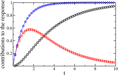
which agrees with the result obtained by solving and then averaging the perturbed equations of motion. In Fig. 1 we compare results of numerical simulations of Eqs. (6-8) with analytical formulas (11-13). On the scale of the figure, the simulation results are indistinguishable from the analytical predictions.

We note that although for the constant force perturbation weighting function p1(t)subscript𝑝1𝑡p_{1}(t) vanishes, to get the linear response we need to include the term τpx˙(t)q1(t)subscript𝜏𝑝delimited-⟨⟩˙𝑥𝑡subscript𝑞1𝑡\tau_{p}\left<\dot{x}(t)q_{1}(t)\right>, which implies that even in this case our method is different from that of Warren and Allen [7].
Refer to caption
Figure 1: The response of the average position to the constant force perturbation, dx(t)λ1/dλ1𝑑subscriptdelimited-⟨⟩𝑥𝑡subscript𝜆1𝑑subscript𝜆1d\left<x(t)\right>_{\lambda_{1}}/d\lambda_{1}. Symbols: results of numerical simulations of Eqs. (6-8) for k=1𝑘1k=1 and τp=3subscript𝜏𝑝3\tau_{p}=3. Circles: x(t)q1(t)delimited-⟨⟩𝑥𝑡subscript𝑞1𝑡\left<x(t)q_{1}(t)\right>, squares: τpx˙(t)q1(t)subscript𝜏𝑝delimited-⟨⟩˙𝑥𝑡subscript𝑞1𝑡\tau_{p}\left<\dot{x}(t)q_{1}(t)\right>, diamonds: complete response. The lines show the analytical formulas, Eqs. (11-13).

In the second example, we perturb the force constant in Eq. (6), kkλ2𝑘𝑘subscript𝜆2k\rightarrow k-\lambda_{2}. The change of the force constant does not change the average position of the self-propelled particle. Instead, it changes the spatial extend of the particle’s steady-state distribution, and the most interesting linear response function measures the change of the average square position of the particle at time t𝑡t after the perturbation was turned on, dx2(t)λ2/dλ2𝑑subscriptdelimited-⟨⟩superscript𝑥2𝑡subscript𝜆2𝑑subscript𝜆2d\left<x^{2}(t)\right>_{\lambda_{2}}/d\lambda_{2}. In this case, Fλ2/λ2=xsubscript𝐹subscript𝜆2subscript𝜆2𝑥\partial F_{\lambda_{2}}/\partial\lambda_{2}=x and 2Fλ2/xλ2=1superscript2subscript𝐹subscript𝜆2𝑥subscript𝜆21\partial^{2}F_{\lambda_{2}}/\partial x\partial\lambda_{2}=1, and thus equations of motion for weights q2(t)subscript𝑞2𝑡q_{2}(t) and p2(t)subscript𝑝2𝑡p_{2}(t) read

q˙2subscript˙𝑞2\displaystyle\dot{q}_{2} =\displaystyle= (2ξ02Teffsp)1xηsuperscript2superscriptsubscript𝜉02superscriptsubscript𝑇effsp1𝑥𝜂\displaystyle\left(2\xi_{0}^{2}T_{\mathrm{eff}}^{\mathrm{sp}}\right)^{-1}x\eta (14)
p˙2subscript˙𝑝2\displaystyle\dot{p}_{2} =\displaystyle= (2ξ03Teffsp)1τp(kx+f)η,superscript2superscriptsubscript𝜉03superscriptsubscript𝑇effsp1subscript𝜏𝑝𝑘𝑥𝑓𝜂\displaystyle\left(2\xi_{0}^{3}T_{\mathrm{eff}}^{\mathrm{sp}}\right)^{-1}\tau_{p}\left(-kx+f\right)\eta, (15)

where Itô prescription is implied. To calculate dx2(t)λ2/dλ2𝑑subscriptdelimited-⟨⟩superscript𝑥2𝑡subscript𝜆2𝑑subscript𝜆2d\left<x^{2}(t)\right>_{\lambda_{2}}/d\lambda_{2}, we need to evaluate weighted averages x2(t)q2(t)delimited-⟨⟩superscript𝑥2𝑡subscript𝑞2𝑡\left<x^{2}(t)q_{2}(t)\right>, x2(t)p2(t)delimited-⟨⟩superscript𝑥2𝑡subscript𝑝2𝑡\left<x^{2}(t)p_{2}(t)\right>, and τpx2˙(t)q2(t)2τpx˙(t)x(t)q2(t)subscript𝜏𝑝delimited-⟨⟩˙superscript𝑥2𝑡subscript𝑞2𝑡2subscript𝜏𝑝delimited-⟨⟩˙𝑥𝑡𝑥𝑡subscript𝑞2𝑡\tau_{p}\left<\dot{x^{2}}(t)q_{2}(t)\right>\equiv 2\tau_{p}\left<\dot{x}(t)x(t)q_{2}(t)\right>. Analytically, it is convenient to evaluate these averages using the exact equation of motion for the joint probability distribution of x𝑥x, f𝑓f, q2subscript𝑞2q_{2} and p2subscript𝑝2p_{2} that can be obtained from Eqs. (6-7) and (14-15). The resulting expressions, consisting of exponential functions, are rather long. Here we present only the final formula for the linear response,

dx2(t)λ2dλ2=1e2kt/ξ0kx2+[1e(k+ξ0/τp)t/ξ0k(k+ξ0/τp)\displaystyle\!\!\!\!\!\!\!\!\!\!\!\!\!\!\!\!\frac{d\left<x^{2}(t)\right>_{\lambda_{2}}}{d\lambda_{2}}=\frac{1-e^{-2kt/\xi_{0}}}{k}\left<x^{2}\right>+\left[\frac{1-e^{-(k+\xi_{0}/\tau_{p})t/\xi_{0}}}{k(k+\xi_{0}/\tau_{p})}\right. (16)
e(k+ξ0/τp)t/ξ0e2kt/ξ0k(kξ0/τp)]xf.\displaystyle\left.-\frac{e^{-(k+\xi_{0}/\tau_{p})t/\xi_{0}}-e^{-2kt/\xi_{0}}}{k(k-\xi_{0}/\tau_{p})}\right]\left<xf\right>.

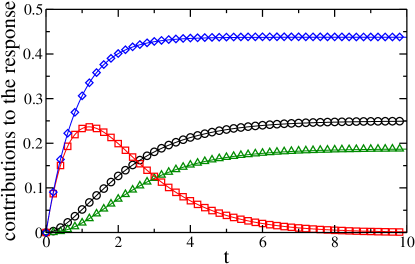
In Fig. 2 we compare the results of numerical simulations of Eqs. (6-7) and (14-15) with the analytical predictions. Again, the simulation and analytical results are indistinguishable.
Refer to caption
Figure 2: The response of the average square position to a change in the force constant, dx2(t)λ2/dλ2𝑑subscriptdelimited-⟨⟩superscript𝑥2𝑡subscript𝜆2𝑑subscript𝜆2d\left<x^{2}(t)\right>_{\lambda_{2}}/d\lambda_{2}. Symbols: results of numerical simulations of Eqs. (6-7) and (14-15) for k=1𝑘1k=1 and τp=3subscript𝜏𝑝3\tau_{p}=3. Circles: x2(t)q2(t)delimited-⟨⟩superscript𝑥2𝑡subscript𝑞2𝑡\left<x^{2}(t)q_{2}(t)\right>, triangles: x2(t)p2(t)delimited-⟨⟩superscript𝑥2𝑡subscript𝑝2𝑡\left<x^{2}(t)p_{2}(t)\right>, squares: τpx2˙(t)q2(t)subscript𝜏𝑝delimited-⟨⟩˙superscript𝑥2𝑡subscript𝑞2𝑡\tau_{p}\left<\dot{x^{2}}(t)q_{2}(t)\right>, diamonds: complete response. The lines show the analytical predictions.

Interestingly, the response of the average position to the constant force perturbation, Eq. (13), is independent of the persistence time of the self-propulsion and is exactly the same as that of a thermal Brownian particle in a harmonic potential. In contrast, the response of the average square position to a change in the force constant depends on the persistence time. In particular, the expressions for the long-time asymptotic responses read

limtdx(t)λ1dλ1subscript𝑡𝑑subscriptdelimited-⟨⟩𝑥𝑡subscript𝜆1𝑑subscript𝜆1\displaystyle\lim_{t\to\infty}\frac{d\left<x(t)\right>_{\lambda_{1}}}{d\lambda_{1}} =\displaystyle= 1k,1𝑘\displaystyle\frac{1}{k}, (17)
limtdx2(t)λ2dλ2subscript𝑡𝑑subscriptdelimited-⟨⟩superscript𝑥2𝑡subscript𝜆2𝑑subscript𝜆2\displaystyle\lim_{t\to\infty}\frac{d\left<x^{2}(t)\right>_{\lambda_{2}}}{d\lambda_{2}} =\displaystyle= Teffsp(1+2kτp/ξ0)k2(1+kτp/ξ0)2.superscriptsubscript𝑇effsp12𝑘subscript𝜏𝑝subscript𝜉0superscript𝑘2superscript1𝑘subscript𝜏𝑝subscript𝜉02\displaystyle\frac{T_{\mathrm{eff}}^{\mathrm{sp}}\left(1+2k\tau_{p}/\xi_{0}\right)}{k^{2}\left(1+k\tau_{p}/\xi_{0}\right)^{2}}. (18)

For a thermal Brownian particle in a harmonic potential the long-time asymptotic responses can be expressed in terms of equilibrium correlations, limtdx(t)λ1eq/dλ1=x2eq/Tsubscript𝑡𝑑superscriptsubscriptdelimited-⟨⟩𝑥𝑡subscript𝜆1eq𝑑subscript𝜆1superscriptdelimited-⟨⟩superscript𝑥2eq𝑇\lim_{t\to\infty}d\left<x(t)\right>_{\lambda_{1}}^{\mathrm{eq}}/d\lambda_{1}=\left<x^{2}\right>^{\mathrm{eq}}/T and limtdx2(t)λ2eq/dλ2=x2(x2x2eq)eq/(2T)subscript𝑡𝑑superscriptsubscriptdelimited-⟨⟩superscript𝑥2𝑡subscript𝜆2eq𝑑subscript𝜆2superscriptdelimited-⟨⟩superscript𝑥2superscript𝑥2superscriptdelimited-⟨⟩superscript𝑥2eqeq2𝑇\lim_{t\to\infty}d\left<x^{2}(t)\right>_{\lambda_{2}}^{\mathrm{eq}}/d\lambda_{2}=\left<x^{2}\left(x^{2}-\left<x^{2}\right>^{\mathrm{eq}}\right)\right>^{\mathrm{eq}}/(2T), where λieqsubscriptsuperscriptdelimited-⟨⟩eqsubscript𝜆𝑖\left<\dots\right>^{\mathrm{eq}}_{\lambda_{i}} denotes a perturbed equilibrium canonical average at temperature T and eqsuperscriptdelimited-⟨⟩eq\left<\dots\right>^{\mathrm{eq}} denotes the un-perturbed equilibrium canonical average. For the self-propelled particle in a harmonic potential these correlations can be calculated analytically,

x2delimited-⟨⟩superscript𝑥2\displaystyle\left<x^{2}\right> =\displaystyle= Teffspk(1+kτp/ξ0),superscriptsubscript𝑇effsp𝑘1𝑘subscript𝜏𝑝subscript𝜉0\displaystyle\frac{T_{\mathrm{eff}}^{\mathrm{sp}}}{k\left(1+k\tau_{p}/\xi_{0}\right)}, (19)
x2(x2x2)delimited-⟨⟩superscript𝑥2superscript𝑥2delimited-⟨⟩superscript𝑥2\displaystyle\left<x^{2}\left(x^{2}-\left<x^{2}\right>\right)\right> =\displaystyle= 2(Teffsp)2k2(1+kτp/ξ0)2.2superscriptsuperscriptsubscript𝑇effsp2superscript𝑘2superscript1𝑘subscript𝜏𝑝subscript𝜉02\displaystyle\frac{2\left(T_{\mathrm{eff}}^{\mathrm{sp}}\right)^{2}}{k^{2}\left(1+k\tau_{p}/\xi_{0}\right)^{2}}. (20)

We note that the right-hand-side of Eq. (19) divided by Teffspsuperscriptsubscript𝑇effspT_{\mathrm{eff}}^{\mathrm{sp}} underestimates the response (17) and likewise the right-hand-side of Eq. (20) divided by 2Teffsp2superscriptsubscript𝑇effsp2T_{\mathrm{eff}}^{\mathrm{sp}} underestimates the response (18).

4 Application

As an application to a system for which exact analytical formulas cannot be obtained, we evaluated the time-dependent mobility of a single particle in a system of interacting self-propelled particles. The mobility function describes the change of the position of a single particle after the application of a weak force. Specifically, at t=0𝑡0t=0 a constant force is applied to particle number 1, F1(𝐫1)F1(𝐫1)+λ𝐞αsubscript𝐹1subscript𝐫1subscript𝐹1subscript𝐫1𝜆subscript𝐞𝛼F_{1}(\mathbf{r}_{1})\rightarrow F_{1}(\mathbf{r}_{1})+\lambda\mathbf{e}_{\alpha}. Here 𝐫isubscript𝐫𝑖\mathbf{r}_{i} is the position of particle i𝑖i, Fi(𝐫i)subscript𝐹𝑖subscript𝐫𝑖F_{i}(\mathbf{r}_{i}) is the interparticle force acting on particle i𝑖i, Fi(𝐫i)=𝐫il>mV(rlm)subscript𝐹𝑖subscript𝐫𝑖subscriptsubscript𝐫𝑖subscript𝑙𝑚𝑉subscript𝑟𝑙𝑚F_{i}(\mathbf{r}_{i})=-\partial_{\mathbf{r}_{i}}\sum_{l>m}V(r_{lm}), with V(r)𝑉𝑟V(r) being the potential, and 𝐞αsubscript𝐞𝛼\mathbf{e}_{\alpha} is a unit vector in the Cartesian direction α𝛼\alpha, α=x,y,z𝛼𝑥𝑦𝑧\alpha=x,y,z. Under the influence of the constant force, particle 1 starts moving and the α𝛼\alpha component of its position starts changing in a systematic way,

α1(t)λ=χ(t)λ+o(λ),subscriptdelimited-⟨⟩subscript𝛼1𝑡𝜆𝜒𝑡𝜆𝑜𝜆\displaystyle\left<\alpha_{1}(t)\right>_{\lambda}=\chi(t)\lambda+o(\lambda), (21)

where χ(t)𝜒𝑡\chi(t) is the mobility function. In the long-time limit, particle 111 achieves a constant velocity and then α𝛼\alpha component of its position changes linearly with time. This allows us to define mobility coefficient μ𝜇\mu,

α1(t)λμtλ for t1.similar-tosubscriptdelimited-⟨⟩subscript𝛼1𝑡𝜆𝜇𝑡𝜆 for 𝑡much-greater-than1\displaystyle\left<\alpha_{1}(t)\right>_{\lambda}\sim\mu t\lambda\text{ for }t\gg 1. (22)

In general, μ𝜇\mu depends on the density, the single-particle effective temperature and the persistence time. Its inverse is the single-particle friction coefficient, ξ=1/μ𝜉1𝜇\xi=1/\mu.

We evaluated the mobility function for a d=3𝑑3d=3 dimensional system of N=1372𝑁1372N=1372 AOUPs interacting via a screened-Coulomb potential, V(r)=Aexp(κ(rσ))/r𝑉𝑟𝐴𝜅𝑟𝜎𝑟V(r)=A\exp\left(-\kappa(r-\sigma)\right)/r, with A=475Teffspσ𝐴475superscriptsubscript𝑇effsp𝜎A=475T_{\mathrm{eff}}^{\mathrm{sp}}\sigma and κσ=24𝜅𝜎24\kappa\sigma=24, at number density Nσ3/V=0.51𝑁superscript𝜎3𝑉0.51N\sigma^{3}/V=0.51. The parameters were chosen in such a way that in the limit of vanishing persistence time the present system becomes equivalent to a colloidal system that we investigated in the past [17]. In the following we use reduced units, with σ𝜎\sigma being the unit of length and σ2ξ0/Teffspsuperscript𝜎2subscript𝜉0superscriptsubscript𝑇effsp\sigma^{2}\xi_{0}/T_{\mathrm{eff}}^{\mathrm{sp}} being the unit of time. We note that the system we considered is rather dense and its steady-state structure factor, for all persistence times investigated, for small wavevectors is approximately constant and small. This suggests that this system does not undergo a phase separation into a dilute and dense components, at least for the persistence times investigated.

The most direct application of the approach presented here would be to run an un-perturbed simulation and, starting at t=0𝑡0t=0, monitor the weighting function q1α(t)subscript𝑞1𝛼𝑡q_{1\alpha}(t), which evolves according to equation of motion

q˙1α=(2ξ02Teffsp)1η1α,subscript˙𝑞1𝛼superscript2superscriptsubscript𝜉02superscriptsubscript𝑇effsp1subscript𝜂1𝛼\displaystyle\dot{q}_{1\alpha}=\left(2\xi_{0}^{2}T_{\mathrm{eff}}^{\mathrm{sp}}\right)^{-1}\eta_{1\alpha}, (23)

where ηiαsubscript𝜂𝑖𝛼\eta_{i\alpha} is the α𝛼\alpha component of the noise acting on the self-propulsion of particle i𝑖i. Then, to get the response function one would need to evaluate α1(t)q1α(t)+τpα˙1(t)q1α(t)delimited-⟨⟩subscript𝛼1𝑡subscript𝑞1𝛼𝑡subscript𝜏𝑝delimited-⟨⟩subscript˙𝛼1𝑡subscript𝑞1𝛼𝑡\left<\alpha_{1}(t)q_{1\alpha}(t)\right>+\tau_{p}\left<\dot{\alpha}_{1}(t)q_{1\alpha}(t)\right>. In practice, it is advantageous to monitor 3N3𝑁3N weighting functions corresponding to all particles and all Cartesian directions, and to average over time origins. This results in the following expression for the mobility function,

χ(t)𝜒𝑡\displaystyle\chi(t) =\displaystyle= 1dNNt0t0,α,i[αi(t)(qiα(t+t0)qiα(t0)\displaystyle\frac{1}{dNN_{t_{0}}}\sum_{t_{0},\alpha,i}\left[\left<\alpha_{i}(t)(q_{i\alpha}(t+t_{0})-q_{i\alpha}(t_{0})\right>\right. (24)
+τpα˙i(t)(qiα(t+t0)qiα(t0)],\displaystyle\left.+\tau_{p}\left<\dot{\alpha}_{i}(t)(q_{i\alpha}(t+t_{0})-q_{i\alpha}(t_{0})\right>\right],

where Nt0subscript𝑁subscript𝑡0N_{t_{0}} is the number of time origins.

We should emphasize at this point that it is averaging over time origins that makes it possible to efficiently calculate the response function from a single unperturbed trajectory.
Refer to caption
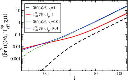
Figure 3: Time dependence of Teffspχ(t)superscriptsubscript𝑇effsp𝜒𝑡T_{\mathrm{eff}}^{\mathrm{sp}}\chi(t) (solid lines) and MSD/6 (dashed lines). Thin lines show τp=0.01subscript𝜏𝑝0.01\tau_{p}=0.01 and thick lines show τp=1subscript𝜏𝑝1\tau_{p}=1. The figure shows that the effective temperature based on the Einstein relation, TeffE=D/μsuperscriptsubscript𝑇effE𝐷𝜇T_{\mathrm{eff}}^{\mathrm{E}}=D/\mu, is close to Teffspsuperscriptsubscript𝑇effspT_{\mathrm{eff}}^{\mathrm{sp}} for τp=0.01subscript𝜏𝑝0.01\tau_{p}=0.01 and is notably smaller than Teffspsuperscriptsubscript𝑇effspT_{\mathrm{eff}}^{\mathrm{sp}} for τp=1subscript𝜏𝑝1\tau_{p}=1.

For a system in thermal equilibrium, mobility function χ(t)𝜒𝑡\chi(t) is simply related to the mean-square displacement (MSD),

Tχ(t)=(2d)1(𝐫i(t)𝐫i(0))2eq.𝑇𝜒𝑡superscript2𝑑1subscriptdelimited-⟨⟩superscriptsubscript𝐫𝑖𝑡subscript𝐫𝑖02eq\displaystyle T\chi(t)=\left(2d\right)^{-1}\left<\left(\mathbf{r}_{i}(t)-\mathbf{r}_{i}(0)\right)^{2}\right>_{\mathrm{eq}}. (25)

In the long-time limit the MSD grows as 2dDt2𝑑𝐷𝑡2dDt, with D𝐷D being the self-diffusion coefficient. Combining definition of the mobility (22) and the asymptotic time-dependence of the MSD we get the Einstein relation, Tμ=D𝑇𝜇𝐷T\mu=D. This relation is, in general, not valid outside of thermal equilibrium.

The Einstein relation can, however, be used to define the following effective temperature

TeffE=D/μ.superscriptsubscript𝑇effE𝐷𝜇\displaystyle T_{\mathrm{eff}}^{\mathrm{E}}=D/\mu. (26)

Here the superscript EE\mathrm{E} indicates that TeffEsuperscriptsubscript𝑇effET_{\mathrm{eff}}^{\mathrm{E}} is defined through the Einstein relation. This effective temperature depends on the density, the single-particle effective temperature and the persistence time, and in general it is different than Teffspsuperscriptsubscript𝑇effspT_{\mathrm{eff}}^{\mathrm{sp}}, except in the low density or vanishing persistence time limits. We showed previously that for a sheared Brownian system TeffEsuperscriptsubscript𝑇effET_{\mathrm{eff}}^{\mathrm{E}} determines the density distribution in a slowly varying external potential beyond linear response [18]. It would be interesting to investigate whether this is also true for an AOUPs system.

In Fig. 3 we compare mobility Teffspχ(t)superscriptsubscript𝑇effsp𝜒𝑡T_{\mathrm{eff}}^{\mathrm{sp}}\chi(t) and the MSD/6 for two values of the persistence time, τp=0.01subscript𝜏𝑝0.01\tau_{p}=0.01 and τp=1subscript𝜏𝑝1\tau_{p}=1. For short times these two functions are notably different. In fact, it can be showed that in the short-time limit χ(t)𝜒𝑡\chi(t) grows linearly with time whereas the MSD grows quadratically with time. In the long time limit both functions grow linearly with time. It can be seen the long time limits of Teffspχ(t)superscriptsubscript𝑇effsp𝜒𝑡T_{\mathrm{eff}}^{\mathrm{sp}}\chi(t) and MSD/6 are very close for τp=0.01subscript𝜏𝑝0.01\tau_{p}=0.01 and markedly different for τp=1subscript𝜏𝑝1\tau_{p}=1. This implies that for τp=0.01subscript𝜏𝑝0.01\tau_{p}=0.01 the effective temperature TeffEsuperscriptsubscript𝑇effET_{\mathrm{eff}}^{\mathrm{E}} is close to Teffspsuperscriptsubscript𝑇effspT_{\mathrm{eff}}^{\mathrm{sp}} whereas for τp=1subscript𝜏𝑝1\tau_{p}=1 these two temperatures are different.
Refer to caption    Refer to caption

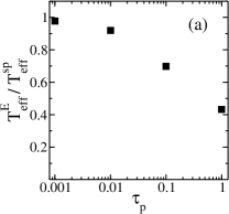
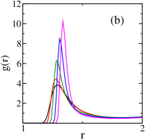
Figure 4: (a) Reduced effective temperature defined through the Einstein relation, TeffE/Teffspsuperscriptsubscript𝑇effEsuperscriptsubscript𝑇effspT_{\mathrm{eff}}^{\mathrm{E}}/T_{\mathrm{eff}}^{\mathrm{sp}}, as a function of persistence time, τpsubscript𝜏𝑝\tau_{p}. (b) Dependence of pair distribution function g(r)𝑔𝑟g(r) on persistence time τpsubscript𝜏𝑝\tau_{p}. The lines represent, from top to bottom, τp=1,0.1,0.01,0.001subscript𝜏𝑝10.10.010.001\tau_{p}=1,0.1,0.01,0.001 and the Brownian limit τp0subscript𝜏𝑝0\tau_{p}\to 0.

In Fig. 4a we show the persistence time dependence of the effective temperature defined through the Einstein relation. For a range of persistence times TeffEsuperscriptsubscript𝑇effET_{\mathrm{eff}}^{\mathrm{E}} changes rather slowly. Then, TeffEsuperscriptsubscript𝑇effET_{\mathrm{eff}}^{\mathrm{E}} starts changing more rapidly and it reaches approximately Teffsp/2superscriptsubscript𝑇effsp2T_{\mathrm{eff}}^{\mathrm{sp}}/2 when the persistence length of the active motion, lpTeffspτp/ξ0similar-tosubscript𝑙𝑝superscriptsubscript𝑇effspsubscript𝜏𝑝subscript𝜉0l_{p}\sim\sqrt{T_{\mathrm{eff}}^{\mathrm{sp}}\tau_{p}/\xi_{0}}, becomes comparable to the range of the potential.

Interestingly, the dependence of the effective temperature defined through the Einstein relation on the persistence time of the self-propulsion is the opposite of that obtained by Levis and Berthier [19] for the system of self-propelled hard disks evolving with Monte Carlo dynamics. Other evidence of a non-universal dependence of the properties of active systems on the departure from thermal equilibrium was noted earlier in Ref. [16].

In Fig. 4b we show the τpsubscript𝜏𝑝\tau_{p} dependence of the simplest structural quantity, the pair distribution function g(r)𝑔𝑟g(r) [1, 2]. Even for the shortest persistence time investigated, τp=0.001subscript𝜏𝑝0.001\tau_{p}=0.001, the height of the first peak of g(r)𝑔𝑟g(r) is markedly different from its value for the thermal Brownian system.

The results showed in Fig. 4 are consistent with results obtained by Fodor et al. [13]. They found that for a range of persistence times the main effect of the departure from equilibrium is a renormalization of the interaction potential. This has a profound influence on the local structure but does not change the effective temperature defined through the Einstein relation.

5 Discussion

We have presented here a method to calculate linear response functions for a class of self-propelled systems from un-perturbed simulations. Our approach generalizes the Malliavin weights method to systems evolving under the influence of a persistent noise. The method can be easily applied to calculate the response of an AOUPs system to a periodic in space time-independent potential [19]. This will allow us to study the wave-vector dependence of effective temperatures. We would also like to investigate the response to an externally imposed shear flow. This will allow us to study the linear viscoelastic properties of active systems. Finally, it would be interesting to investigate whether the approach presented here could be generalized to calculate directly the frequency-dependent response, i.e. response to a perturbation periodic in time [9], and to calculate directly linear response functions for systems of active Brownian particles, without relying on the mapping procedure proposed in Ref. [14].

6 Acknowledgments

Most of this work was done when I was visiting Laboratoire Charles Coulomb of Université de Montpellier. The hospitality of the Laboratoire was greatly appreciated. The research in Montpellier is supported by funding from the European Research Council under the European Union’s Seventh Framework Programme (FP7/2007-2013) / ERC Grant agreement No 306845. I also gratefully acknowledge the support of NSF Grant No. CHE 1213401. I thank E. Flenner for comments on the manuscript.

7 Appendix: derivation of the main result

To evaluate the dependence of Φ(x;t)λsubscriptdelimited-⟨⟩Φ𝑥𝑡𝜆\left<\Phi(x;t)\right>_{\lambda} on λ𝜆\lambda we follow the strategy inspired by Sec. 2 of Ref. [8]. Specifically, we write Φ(x;t)λsubscriptdelimited-⟨⟩Φ𝑥𝑡𝜆\left<\Phi(x;t)\right>_{\lambda} as

Φ(x;t)λ=subscriptdelimited-⟨⟩Φ𝑥𝑡𝜆absent\displaystyle\left<\Phi(x;t)\right>_{\lambda}= (27)
𝑑xN𝑑fN𝑑x0𝑑f0Φ(xN)Pλ(xN,fN|xN1,fN1;Δt)differential-dsubscript𝑥𝑁differential-dsubscript𝑓𝑁differential-dsubscript𝑥0differential-dsubscript𝑓0Φsubscript𝑥𝑁subscript𝑃𝜆subscript𝑥𝑁conditionalsubscript𝑓𝑁subscript𝑥𝑁1subscript𝑓𝑁1Δ𝑡\displaystyle\int dx_{N}df_{N}...dx_{0}df_{0}\Phi(x_{N})P_{\lambda}(x_{N},f_{N}|x_{N-1},f_{N-1};\Delta t)
×Pλ(x1,f1|x0,f0;Δt)Pss(x0,f0),absentsubscript𝑃𝜆subscript𝑥1conditionalsubscript𝑓1subscript𝑥0subscript𝑓0Δ𝑡superscript𝑃𝑠𝑠subscript𝑥0subscript𝑓0\displaystyle\times\dots P_{\lambda}(x_{1},f_{1}|x_{0},f_{0};\Delta t)P^{ss}(x_{0},f_{0}),

where for 1<i1𝑖1<i Pλ(xi,vi|xi1,fi1;Δt)subscript𝑃𝜆subscript𝑥𝑖conditionalsubscript𝑣𝑖subscript𝑥𝑖1subscript𝑓𝑖1Δ𝑡P_{\lambda}(x_{i},v_{i}|x_{i-1},f_{i-1};\Delta t) is the transition probability over small interval Δt=t/NΔ𝑡𝑡𝑁\Delta t=t/N, corresponding to the evolution equations (1-2) with modified force Fλsubscript𝐹𝜆F_{\lambda},

Pλ(xi,fi|xi1,fi1;Δt)=subscript𝑃𝜆subscript𝑥𝑖conditionalsubscript𝑓𝑖subscript𝑥𝑖1subscript𝑓𝑖1Δ𝑡absent\displaystyle P_{\lambda}(x_{i},f_{i}|x_{i-1},f_{i-1};\Delta t)= (28)
δ(xixi1(Fλ(xi1)+fi1)Δt/ξ0)𝛿subscript𝑥𝑖subscript𝑥𝑖1subscript𝐹𝜆subscript𝑥𝑖1subscript𝑓𝑖1Δ𝑡subscript𝜉0\displaystyle\delta\left(x_{i}-x_{i-1}-(F_{\lambda}(x_{i-1})+f_{i-1})\Delta t/\xi_{0}\right)
×exp((fifi1+fi1Δt/τp)24ξ0TeffspΔt/τp2)4πξ0TeffspΔt/τp2,absentsuperscriptsubscript𝑓𝑖subscript𝑓𝑖1subscript𝑓𝑖1Δ𝑡subscript𝜏𝑝24subscript𝜉0superscriptsubscript𝑇effspΔ𝑡superscriptsubscript𝜏𝑝24𝜋subscript𝜉0superscriptsubscript𝑇effspΔ𝑡superscriptsubscript𝜏𝑝2\displaystyle\times\frac{\exp\left(-\frac{(f_{i}-f_{i-1}+f_{i-1}\Delta t/\tau_{p})^{2}}{4\xi_{0}T_{\mathrm{eff}}^{\mathrm{sp}}\Delta t/\tau_{p}^{2}}\right)}{\sqrt{4\pi\xi_{0}T_{\mathrm{eff}}^{\mathrm{sp}}\Delta t/\tau_{p}^{2}}},

Pλ(x1,v1|x0,f0;Δt)subscript𝑃𝜆subscript𝑥1conditionalsubscript𝑣1subscript𝑥0subscript𝑓0Δ𝑡P_{\lambda}(x_{1},v_{1}|x_{0},f_{0};\Delta t) is the transition probability with the un-modified force F𝐹F, and Pss(x0,f0)superscript𝑃𝑠𝑠subscript𝑥0subscript𝑓0P^{ss}(x_{0},f_{0}) is the steady state distribution for the un-perturbed system (i.e. the system evolving under the influence of force F𝐹F).

At this point it is convenient to change the integration variables for 0<i<N0𝑖𝑁0<i<N from (xi,fi)subscript𝑥𝑖subscript𝑓𝑖(x_{i},f_{i}) to (xi,wi)subscript𝑥𝑖subscript𝑤𝑖(x_{i},w_{i}), where wi=Fλ(xi)+fisubscript𝑤𝑖subscript𝐹𝜆subscript𝑥𝑖subscript𝑓𝑖w_{i}=F_{\lambda}(x_{i})+f_{i}. Next, one differentiates both sides of Eq. (27) w.r.t. λ𝜆\lambda. Then, after some transformations, one changes the variables back to the original variables and one obtains the following equation

ddλΦ(x;t)λ=𝑑xN𝑑fN𝑑x0𝑑f0Φ(xN)𝑑𝑑𝜆subscriptdelimited-⟨⟩Φ𝑥𝑡𝜆differential-dsubscript𝑥𝑁differential-dsubscript𝑓𝑁differential-dsubscript𝑥0differential-dsubscript𝑓0Φsubscript𝑥𝑁\displaystyle\!\!\!\!\!\!\!\!\!\!\frac{d}{d\lambda}\left<\Phi(x;t)\right>_{\lambda}=\int dx_{N}df_{N}...dx_{0}df_{0}\Phi(x_{N})
×[(fNfN1+fN1Δt/τp)2ξ02TeffspΔt/τp2(1Δtτp)Fλ(xN1)λ\displaystyle\!\!\!\!\!\!\!\!\!\!\!\!\times\left[-\frac{(f_{N}-f_{N-1}+f_{N-1}\Delta t/\tau_{p})}{2\xi_{0}^{2}T_{\mathrm{eff}}^{\mathrm{sp}}\Delta t/\tau_{p}^{2}}\left(1-\frac{\Delta t}{\tau_{p}}\right)\frac{\partial F_{\lambda}(x_{N-1})}{\partial\lambda}\right.
+i=1N1(fifi1+fi1Δt/τp)2ξ02TeffspΔt/τp2(2Fλ(xi1)xi1λxixi1Δt)Δtsuperscriptsubscript𝑖1𝑁1subscript𝑓𝑖subscript𝑓𝑖1subscript𝑓𝑖1Δ𝑡subscript𝜏𝑝2superscriptsubscript𝜉02superscriptsubscript𝑇effspΔ𝑡superscriptsubscript𝜏𝑝2superscript2subscript𝐹𝜆subscript𝑥𝑖1subscript𝑥𝑖1𝜆subscript𝑥𝑖subscript𝑥𝑖1Δ𝑡Δ𝑡\displaystyle\!\!\!\!\!\!\!\!\!\!\!\!\left.+\sum_{i=1}^{N-1}\frac{(f_{i}-f_{i-1}+f_{i-1}\Delta t/\tau_{p})}{2\xi_{0}^{2}T_{\mathrm{eff}}^{\mathrm{sp}}\Delta t/\tau_{p}^{2}}\left(\frac{\partial^{2}F_{\lambda}(x_{i-1})}{\partial x_{i-1}\partial\lambda}\frac{x_{i}-x_{i-1}}{\Delta t}\right)\Delta t\right.
+i=2N1(fifi1+fi1Δt/τp)2ξ02TeffspΔt/τp(Fλ(xi1)λ)Δtsuperscriptsubscript𝑖2𝑁1subscript𝑓𝑖subscript𝑓𝑖1subscript𝑓𝑖1Δ𝑡subscript𝜏𝑝2superscriptsubscript𝜉02superscriptsubscript𝑇effspΔ𝑡subscript𝜏𝑝subscript𝐹𝜆subscript𝑥𝑖1𝜆Δ𝑡\displaystyle\!\!\!\!\!\!\!\!\!\!\!\!\left.+\sum_{i=2}^{N-1}\frac{(f_{i}-f_{i-1}+f_{i-1}\Delta t/\tau_{p})}{2\xi_{0}^{2}T_{\mathrm{eff}}^{\mathrm{sp}}\Delta t/\tau_{p}}\left(\frac{\partial F_{\lambda}(x_{i-1})}{\partial\lambda}\right)\Delta t\right.
+(f1f0+f0Δt/τp)2ξ02TeffspΔt/τp2Fλ(x0)λ]\displaystyle\!\!\!\!\!\!\!\!\!\!\!\!\left.+\frac{(f_{1}-f_{0}+f_{0}\Delta t/\tau_{p})}{2\xi_{0}^{2}T_{\mathrm{eff}}^{\mathrm{sp}}\Delta t/\tau_{p}^{2}}\frac{\partial F_{\lambda}(x_{0})}{\partial\lambda}\right]
×P(xN,fN|xN1,fN1;Δt)P(x1,f1|x0,f0;Δt)absent𝑃subscript𝑥𝑁conditionalsubscript𝑓𝑁subscript𝑥𝑁1subscript𝑓𝑁1Δ𝑡𝑃subscript𝑥1conditionalsubscript𝑓1subscript𝑥0subscript𝑓0Δ𝑡\displaystyle\!\!\!\!\!\!\!\!\!\!\!\!\times P(x_{N},f_{N}|x_{N-1},f_{N-1};\Delta t)\dots P(x_{1},f_{1}|x_{0},f_{0};\Delta t)
×Pss(x0,f0).absentsuperscript𝑃𝑠𝑠subscript𝑥0subscript𝑓0\displaystyle\!\!\!\!\!\!\!\!\!\!\!\!\times P^{ss}(x_{0},f_{0}). (29)

Then, one uses an identity which follows from the time-independence of a the steady state distribution,

𝑑xN𝑑fN𝑑x0𝑑f0Φ(xN)Φ(xN1)Δtdifferential-dsubscript𝑥𝑁differential-dsubscript𝑓𝑁differential-dsubscript𝑥0differential-dsubscript𝑓0Φsubscript𝑥𝑁Φsubscript𝑥𝑁1Δ𝑡\displaystyle\int dx_{N}df_{N}...dx_{0}df_{0}\frac{\Phi(x_{N})-\Phi(x_{N-1})}{\Delta t}
×i=1N1(fifi1+fi1Δt/τp)2ξ02Teffsp/τp2Fλ(xi1)λ\displaystyle\times\sum_{i=1}^{N-1}\frac{(f_{i}-f_{i-1}+f_{i-1}\Delta t/\tau_{p})}{2\xi_{0}^{2}T_{\mathrm{eff}}^{\mathrm{sp}}/\tau_{p}^{2}}\frac{\partial F_{\lambda}(x_{i-1})}{\partial\lambda}
×P(xN,fN|xN1,fN1;Δt)P(x1,f1|x0,f0;Δt)absent𝑃subscript𝑥𝑁conditionalsubscript𝑓𝑁subscript𝑥𝑁1subscript𝑓𝑁1Δ𝑡𝑃subscript𝑥1conditionalsubscript𝑓1subscript𝑥0subscript𝑓0Δ𝑡\displaystyle\times P(x_{N},f_{N}|x_{N-1},f_{N-1};\Delta t)...P(x_{1},f_{1}|x_{0},f_{0};\Delta t)
×Pss(x0,f0)=dxNdfNdx0df0Φ(xN)\displaystyle\times P^{ss}(x_{0},f_{0})=\int dx_{N}df_{N}...dx_{0}df_{0}\Phi(x_{N})
[(fNfN1+fN1Δt/τp)2ξ02TeffspΔt/τp2Fλ(xN1)λ\displaystyle\left[-\frac{(f_{N}-f_{N-1}+f_{N-1}\Delta t/\tau_{p})}{2\xi_{0}^{2}T_{\mathrm{eff}}^{\mathrm{sp}}\Delta t/\tau_{p}^{2}}\frac{\partial F_{\lambda}(x_{N-1})}{\partial\lambda}\right.
+(f1f0+f0Δt/τp)2ξ02TeffspΔt/τp2Fλ(x0)λ]\displaystyle\left.+\frac{(f_{1}-f_{0}+f_{0}\Delta t/\tau_{p})}{2\xi_{0}^{2}T_{\mathrm{eff}}^{\mathrm{sp}}\Delta t/\tau_{p}^{2}}\frac{\partial F_{\lambda}(x_{0})}{\partial\lambda}\right]
×P(xN,fN|xN1,fN1;Δt)P(x1,f1|x0,f0;Δt)absent𝑃subscript𝑥𝑁conditionalsubscript𝑓𝑁subscript𝑥𝑁1subscript𝑓𝑁1Δ𝑡𝑃subscript𝑥1conditionalsubscript𝑓1subscript𝑥0subscript𝑓0Δ𝑡\displaystyle\times P(x_{N},f_{N}|x_{N-1},f_{N-1};\Delta t)\dots P(x_{1},f_{1}|x_{0},f_{0};\Delta t)
×Pss(x0,f0)absentsuperscript𝑃𝑠𝑠subscript𝑥0subscript𝑓0\displaystyle\times P^{ss}(x_{0},f_{0}) (30)

Combining Eqs. (7) and (7) one arrives at the final Eq. (7),

ddλΦ(x;t)λ=𝑑xN𝑑fN𝑑x0𝑑f0𝑑𝑑𝜆subscriptdelimited-⟨⟩Φ𝑥𝑡𝜆differential-dsubscript𝑥𝑁differential-dsubscript𝑓𝑁differential-dsubscript𝑥0differential-dsubscript𝑓0\displaystyle\frac{d}{d\lambda}\left<\Phi(x;t)\right>_{\lambda}=\int dx_{N}df_{N}...dx_{0}df_{0}
{Φ(xN)[i=2N(fifi1+fi1Δt/τp)2ξ02Teffsp/τpFλ(xi1)λ\displaystyle\left\{\Phi(x_{N})\left[\sum_{i=2}^{N}\frac{(f_{i}-f_{i-1}+f_{i-1}\Delta t/\tau_{p})}{2\xi_{0}^{2}T_{\mathrm{eff}}^{\mathrm{sp}}/\tau_{p}}\frac{\partial F_{\lambda}(x_{i-1})}{\partial\lambda}\right.\right.
+i=1N1(fifi1+fi1Δt/τp)2ξ02Teffsp/τp22Fλ(xi)xiλxixi1Δt]\displaystyle\left.\left.+\sum_{i=1}^{N-1}\frac{(f_{i}-f_{i-1}+f_{i-1}\Delta t/\tau_{p})}{2\xi_{0}^{2}T_{\mathrm{eff}}^{\mathrm{sp}}/\tau_{p}^{2}}\frac{\partial^{2}F_{\lambda}(x_{i})}{\partial x_{i}\partial\lambda}\frac{x_{i}-x_{i-1}}{\Delta t}\right]\right.
+Φ(xN)Φ(xN1)Δti=1N1(fifi1+fi1Δt/τp)2ξ02Teffsp/τp2Φsubscript𝑥𝑁Φsubscript𝑥𝑁1Δ𝑡superscriptsubscript𝑖1𝑁1subscript𝑓𝑖subscript𝑓𝑖1subscript𝑓𝑖1Δ𝑡subscript𝜏𝑝2superscriptsubscript𝜉02superscriptsubscript𝑇effspsuperscriptsubscript𝜏𝑝2\displaystyle\left.+\frac{\Phi(x_{N})-\Phi(x_{N-1})}{\Delta t}\sum_{i=1}^{N-1}\frac{(f_{i}-f_{i-1}+f_{i-1}\Delta t/\tau_{p})}{2\xi_{0}^{2}T_{\mathrm{eff}}^{\mathrm{sp}}/\tau_{p}^{2}}\right.
×Fλ(xi1)λ}×P(xN,fN|xN1,fN1;Δt)\displaystyle\left.\times\frac{\partial F_{\lambda}(x_{i-1})}{\partial\lambda}\right\}\times P(x_{N},f_{N}|x_{N-1},f_{N-1};\Delta t)\dots
×P(x1,f1|x0,f0;Δt)Pss(x0,f0).absent𝑃subscript𝑥1conditionalsubscript𝑓1subscript𝑥0subscript𝑓0Δ𝑡superscript𝑃𝑠𝑠subscript𝑥0subscript𝑓0\displaystyle\times P(x_{1},f_{1}|x_{0},f_{0};\Delta t)P^{ss}(x_{0},f_{0}). (31)

In Eqs. (7-7) P(xi,fi|xi1,fi1;Δt)𝑃subscript𝑥𝑖conditionalsubscript𝑓𝑖subscript𝑥𝑖1subscript𝑓𝑖1Δ𝑡P(x_{i},f_{i}|x_{i-1},f_{i-1};\Delta t) is the transition probability corresponding to the un-perturbed evolution. It has the same form as the transition probability (28) but the force is the unperturbed force F(xi1)𝐹subscript𝑥𝑖1F(x_{i-1}).

Assuming that the Δt0Δ𝑡0\Delta t\to 0 limit can be taken, we get our main result, Eq. (3), with weights q(t)𝑞𝑡q(t) and p(t)𝑝𝑡p(t) evolving according to Eqs. (4-5).

References

  • [1] D. Chandler, Introduction to Modern Statistical Mechanics, (Oxford, New York, 1987).
  • [2] J.P. Hansen and I.R. McDonald, Theory of Simple Liquids (Elsevier, Amsterdam, 2006).
  • [3] C. Chatelain, J. Phys. A 36, 10739 (2003).
  • [4] F. Ricci-Tersenghi, Phys. Rev. E 68, 065104 (2003).
  • [5] F. Corberi, E. Lippiello, A. Sarracino, and M. Zannetti, Phys. Rev. E 81, 011124 (2010), and references cited therein.
  • [6] L. Berthier, Phys. Rev. Lett. 98, 220601 (2007).
  • [7] P. Warren and R. Allen, Phys. Rev. Lett. 109, 250601 (2012); Entropy 16, 221 (2014).
  • [8] N. Chen and P. Glasserman, Stoch. Proc. Appl. 117, 1689 (2007).
  • [9] See, e.g., D. Mizuno, C. Tardin, C. F. Schmidt, and F.C. MacKintosh, Science 315, 370 (2007); C. Wilhelm, Phys. Rev. Lett. 101, 028101 (2008); W.W. Ahmed, E. Fodor, and T. Betz, Biochimica et Biophysica Acta 1853, 3083 (2015); and references therein.
  • [10] G. Szamel, Phys. Rev. E 90, 012111 (2014).
  • [11] L. Berthier, Phys. Rev. Lett. 112, 220602 (2014).
  • [12] C. Maggi, U. M. B. Marconi, N. Gnan, and R. Di Leonardo, Sci. Rep. 5, 10742 (2015).
  • [13] E. Fodor, C. Nardini, M. E. Cates, J. Tailleur, P. Visco, and F. van Wijland, Phys. Rev. Lett. 117, 038103 (2016).
  • [14] T. F. F. Farage, P. Krinninger, and J. M. Brader, Phys. Rev. E 91, 042310 (2015).
  • [15] B. ten Hagen, S. van Teeffelen, and H. Löwen, J. Phys.: Condens. Matter 23, 194119 (2011).
  • [16] E. Flenner, G. Szamel, and L. Berthier, Soft Matter 12, 7136 (2016).
  • [17] G. Szamel, J. Chem. Phys. 114, 8708 (2001).
  • [18] G. Szamel and M. Zhang, EPL, 96, 50007 (2011).
  • [19] D. Levis and L. Berthier, EPL 111, 60006 (2015).