HATS-19b, HATS-20b, HATS-21b: Three transiting hot-Saturns discovered by the HATSouth survey

Abstract

We report the discovery by the HATSouth exoplanet survey of three hot-Saturn transiting exoplanets: HATS-19b, HATS-20b, and HATS-21b. The planet host HATS-19 is a slightly evolved $V=13.0$ G0 star with enhanced metallicity of $\rm[Fe/H]=0.240\pm 0.050$, a mass of $M_{\star}=1.303\pm 0.083$ $M_{\sun}$ and a radius of $R_{\star}=1.75\pm 0.25$ $R_{\sun}$. HATS-19b is in an eccentric orbit ($e=0.30\pm 0.10$) around this star with an orbital period of $4.5697$ days, and has a mass of $M_{p}=0.427\pm 0.071$ $M_{\rm J}$ and a highly inflated radius of $R_{p}=1.66_{-0.21}^{+0.27}$ $R_{\rm J}$. In contrast, the planet HATS-20b has a Saturn-like mass and radius of $M_{p}=0.273\pm 0.035$ $M_{\rm J}$ and $R_{p}=0.776\pm 0.055$ $R_{\rm J}$ respectively. It orbits the less massive $V=13.8$ G9V star HATS-20 ($M_{\star}=0.910\pm 0.026$ $M_{\sun}$; $R_{\star}=0.892_{-0.040}^{+0.057}$ $R_{\sun}$) with a period of $3.7993$ days. Finally, HATS-21 is a relatively bright G4V star ($V=12.2$ mag) with super-Solar metallicity of $\rm[Fe/H]=0.300\pm 0.040$, a mass of $M_{\star}=1.080\pm 0.026$ $M_{\sun}$, and a radius of $R_{\star}=1.021_{-0.036}^{+0.089}$ $R_{\sun}$. Its accompanying planet HATS-21b has a $3.5544$-day orbital period, a mass of $M_{p}=0.332_{-0.030}^{+0.040}$ $M_{\rm J}$, and a moderately inflated radius of $R_{p}=1.123_{-0.054}^{+0.147}$ $R_{\rm J}$. With the addition of these three very different planets to the growing sample of hot-Saturns, we re-examine the relations between the observed giant planet radii, stellar irradiation, and host metallicity. In agreement with earlier results, we find that there is a significant positive correlation between planet equilibrium temperature and radius, and a weak negative correlation between host metallicity and radius. To assess the relative influence of various physical parameters on the observed planet radii, we train and fit models using Random Forest regression. We find that for hot-Saturns ($0.1<M_{p}<0.5\ M_{\rm J}$), the planetary mass and equilibrium temperature play dominant roles in determining planet radii. In contrast, for hot-Jupiters ($0.5<M_{p}<2.0\ M_{\rm J}$), the most important parameter appears to be equilibrium temperature alone. Finally, for irradiated higher-mass planets ($M_{p}>2.0\ M_{\rm J}$), we find that equilibrium temperature dominates in influence, with smaller contributions from the planet mass, and host metallicity.

1. Introduction

The accelerating rate of discovery of transiting exoplanets in the past decade has been driven by the continuing efforts of ground-based surveys such as HATNet (Bakos et al., 2004), HATSouth (Bakos et al., 2013), WASP (Pollacco et al., 2006), KELT (Pepper et al., 2007), and the important contributions of space missions, including CoRoT (Baglin, 2003) and Kepler (Borucki et al., 2010). It is now becoming increasingly possible to study populations of exoplanets, characterize trends in their properties, and perform robust comparisons to theoretical models of their formulation and evolution. Many of the giant exoplanets (with mass $M_{\rm p}>0.1\ M_{\rm J}$) discovered so far have measured radii that are inflated with respect to Jupiter itself over a large range of planetary masses. This is an expected outcome based on the small orbital semi-major axes of the majority of these planets, which are all significantly affected by stellar irradiation from their host stars. The details of this mechanism, however, are not fully understood. Possible candidates include tidal heating (Jackson et al., 2008), opacity-induced inefficiencies in energy transport in the planet atmosphere (Burrows et al., 2007), and several other methods of depositing energy into the planet interior (Guillot & Showman, 2002; Batygin et al., 2011), thus inflating its radius. The effects of these different mechanisms may differ over a range of planet masses, host star metallicity and luminosity, and orbital eccentricities, thus allowing us to distinguish between them.

The small number of transiting low mass giant planets, particularly hot-Saturns ($0.1<M_{\rm p}<0.5\ M_{\rm J}$), however, makes the determination of any definitive trends of planet radius with planet mass, the level of stellar irradiation, or the host star metallicity, rather difficult. With the focus of space-based transiting exoplanet missions shifting to even lower mass Earth-like planets, ground-based transit surveys have the unique opportunity to deeply explore this parameter space.

In this paper, we report three transiting Saturn-mass exoplanets in close orbit around G stars, HATS-19b, HATS-20b, and HATS-21b, discovered using HATSouth survey observations in 2011 and 2012, and confirmed via subsequent photometric and spectroscopic follow-up observations. The HATSouth survey achieved first light in 2009, and has discovered many interesting transiting exoplanetary systems in the Southern sky since then. Recent highlights include a transiting hot-Saturn in orbit around an M-dwarf (Hartman et al., 2015) and the longest period transiting exoplanet discovered by a ground-based survey so far (Brahm et al., 2016).

The planets discussed in this work are quite diverse in their properties. HATS-19b is one of the most highly inflated giant planets discovered so far, despite its Saturn-like mass. HATS-20b is a planet much like Saturn itself in mass, density, and radius, despite being in close orbit around and under significant irradiation from its host star. Finally, HATS-21b is a significantly inflated Saturn that orbits a relatively metal-rich host star.

This paper is organized as follows. In § 2.1, we describe the initial observations leading to the detection of transits of these three exoplanets. Follow up efforts are described in §  2.2, including reconnaissance spectroscopy, high-precision follow-up light curves, lucky imaging to rule out close companions, and finally, precise radial velocity measurements. We present our analysis in § 3, including determination of the properties of the host stars (§ 3.1), ruling out blends (§ 3.3), and final parameters for HATS-19b, HATS-20b, and HATS-21b (§ 3.4). Finally, in § 4, we discuss these newly discovered planets and investigate the relations between planet radius and stellar irradiation and stellar metallicity for a sample of well-characterized transiting giant exoplanets from the literature, and resulting implications.

2. Observations

2.1. Initial photometric detection

The six robotic HATSouth telescope units, distributed evenly in longitude for near-continuous phase coverage, are located (two units per site) at the Las Campanas Observatory in Chile (LCO), the High Energy Stereoscopic System (HESS) site in Namibia, and the Siding Spring Observatory in Australia (SSO). Each telescope unit consists of four 180-mm aperture f/2.8 Takahashi astrograph telescopes backed by 4K $\times$ 4K Apogee U16M Alta CCDs on a common mount, with a $4^{\circ}\times 4^{\circ}$ field of view per telescope (resulting in a per-unit combined field-of-view of $8^{\circ}\times 8^{\circ}$) and pixel scale of 3$\farcs$7 pixel^-1. The units observe autonomously from dusk to dawn, suspending operations as needed during bad weather. During more than five years of HATSouth operations, we have collected $>3$ million frames for $\sim 10$ million stars to a limiting $r<16$ mag, covering $\sim 13\%$ of the Southern sky.

HATS-19, -20, and -21 are stars observed in the HATSouth primary fields G606 centered at $\alpha=09^{\rm h}36^{\rm m}$, $\delta=-30^{\circ}00^{\prime}$, G700 centered at $\alpha=13^{\rm h}12^{\rm m}$, $\delta=-45^{\circ}00^{\prime}$, and G777 centered at $\alpha=18^{\rm h}24^{\rm m}$, $\delta=-60^{\circ}00^{\prime}$ respectively. Field G606 was observed by the HATSouth units HS-1 at LCO, HS-3 at HESS, and HS-5 at SSO from 2011 January to 2012 June. Additional observations of an overlapping field G607 were taken by the HATSouth units HS-2 at LCO, HS-4 at HESS, and HS-6 at SSO during 2012 February–June. Field G700 was observed by HS-2, HS-4, and HS-6 from 2011 April to 2012 July. Field G777 was observed by HS-1, HS-3, and HS-5 from 2011 May to 2012 September, with additional observations of an overlapping field G778 by HATSouth units HS-2, HS-4, and HS-6 during 2011 May to 2012 October.

All photometric observations were reduced to light curves following the aperture photometry procedures detailed in Bakos et al. (2013) and Penev et al. (2013). Systematics in the light curves were removed using the External Parameter Decorrelation (EPD; Bakos et al. 2010) method and the Trend Filtering Algorithm (TFA; Kovács et al. 2005). These detrended light curves were then searched for exoplanet transit signals using the Box-fitting Least Squares algorithm (BLS; Kovács et al. 2002).

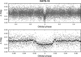
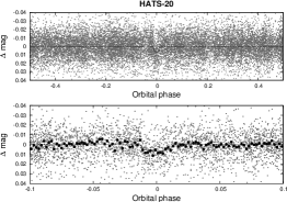
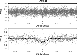
Figure 1.— Phase-folded unbinned HATSouth light curves for HATS-19 (left), HATS-20 (middle) and HATS-21 (right). In each case we show two panels. The top panel shows the full light curve, while the bottom panel shows the light curve zoomed-in on the transit. The solid lines show the model fits to the light curves. The dark filled circles in the bottom panels show the light curves binned in phase with a bin size of 0.002.

We detected a transit signal in combined observations of HATSouth fields G606 and G607 for the star HATS-19 ($\alpha=09^{\rm h}49^{\rm m}37\fs 63$, $\delta=-33^{\circ}13^{\prime}06\farcs 6$, $V=13.030\pm 0.060\ {\rm mag}$, also known as 2MASS J09493761-3313065) with a depth of 10.3 milli-mag (mmag), a period of $4.5697$ days, and duration of $4.005$ hours. In total, 19990 Sloan $r$-band light curve points with 4-minute exposure time were obtained for this object with a median cadence of $\sim 5$ minutes.

Similarly, a transit signal was detected for the star HATS-20 ($\alpha=13^{\rm h}12^{\rm m}32\fs 04$, $\delta=-45^{\circ}35^{\prime}26\farcs 0,V=13.765\pm 0.050\ {\rm mag}$, also known as 2MASS J13123190-4535259) during observations of field G700 with a depth of 8.3 mmag, a period of $3.7993$ days, and transit duration of $2.453$ hours. The light curve for this object has total of 16191 4-minute Sloan $r$-band exposures with a median cadence of $\sim 5$ minutes.

Finally, we detected a transit signal in combined observations of field G777 and G778 for the star HATS-21 ($\alpha=18^{\rm h}40^{\rm m}44\fs 40$, $\delta=-58^{\circ}27^{\prime}33\farcs 3,V=12.191\pm 0.020\ {\rm mag}$, also known as 2MASS J18404426-5827332) with a depth of 11.1 mmag, duration of $1.978$ hours, and a period of $3.5544$ days. The light curve for this object has 13106 4-minute Sloan $r$-band light curve points with a 5-minute median cadence.

Table 1 presents a summary of the various HATSouth photometric observations. Figure 1 shows the discovery light curves, phase-folded at their respective orbital periods, for all three transiting systems.

All transit candidates from HATSouth observations of these fields were then vetted by reconnaissance spectroscopy to determine stellar parameters and rule out large radial velocity variations indicative of eclipsing binaries (§ 2.2.1). HATS-19, -20, and -21 were identified as promising targets for further photometric follow-up observations to obtain high-quality light curves and confirm their transit signals (§ 2.2.2). Finally, high precision radial velocity (RV) measurements were carried out for the three transit candidates (§  2.2.4) to determine their fundamental properties.

Table 1 Summary of photometric observations

Instrument/Field	Date(s)	# Images	Cadence	Filter	Precision
			(sec)		(mmag)
HATS-19
HS-2.4/G606	2012 Feb–2012 Jun	3702	291	$r$	7.8
HS-4.4/G606	2012 Mar–2012 Jun	2154	300	$r$	7.7
HS-6.4/G606	2012 Feb–2012 Jun	1164	299	$r$	9.4
HS-1.1/G607	2011 Jan–2012 Jun	6735	289	$r$	9.2
HS-3.1/G607	2011 Jan–2012 Jun	3180	289	$r$	9.9
HS-5.1/G607	2011 Jan–2012 Apr	3055	288	$r$	9.3
Swope 1 m/site3	2013 Nov 21	117	100	$r$	1.6
DK 1.54 m/DFOSC	2014 Mar 20	104	225	$B$	1.2
Swope 1 m/e2v	2014 Mar 20	168	161	$i$	2.3
HATS-20
HS-2.1/G700	2011 Apr–2012 Jul	2186	292	$r$	19.7
HS-4.1/G700	2011 Jul–2012 Jul	3754	301	$r$	14.4
HS-6.1/G700	2011 May–2012 Jul	854	300	$r$	28.0
HS-2.4/G700	2011 Apr–2012 Jul	4428	292	$r$	11.8
HS-4.4/G700	2011 Jul–2012 Jul	3553	301	$r$	11.0
HS-6.4/G700	2011 May–2012 Jul	1416	300	$r$	12.9
PEST 0.3 m	2015 Apr 23	233	132	$R_{C}$	4.6
LCOGT 1 m+SAAO/SBIG	2015 May 12	86	145	$i$	2.5
LCOGT 1 m+CTIO/sinistro	2015 May 27	70	226	$i$	2.0
Swope 1 m/e2v	2015 May 27	113	159	$i$	1.5
HATS-21
HS-1.3/G777	2011 May–2012 Sep	1519	298	$r$	8.2
HS-3.3/G777	2011 Jul–2012 Sep	1632	297	$r$	7.1
HS-5.3/G777	2011 May–2012 Sep	1000	303	$r$	7.2
HS-2.2/G778	2011 May–2012 Nov	3057	288	$r$	6.0
HS-4.2/G778	2011 Jul–2012 Nov	3707	298	$r$	6.0
HS-6.2/G778	2011 Apr–2012 Oct	2191	298	$r$	7.8
LCOGT 1 m+SAAO/SBIG	2015 Jul 15	90	143	$i$	1.0

2.2. Follow-up observations

2.2.1 Reconnaissance spectroscopy

Reconnaissance spectroscopy was performed for all three targets using the Wide Field Spectrograph (WiFeS; Dopita et al. 2007) instrument on the Australian National University (ANU) 2.3-m telescope at SSO. Details of reductions for these data are presented in Bayliss et al. (2013); we briefly summarize the process:

The first stage of these observations involved a single spectrum taken with modest resolution $R\equiv\lambda/\Delta\lambda=3000$ to determine if the transit candidate stars were dwarfs, as transit signals for giant stars with the measured duration from HATSouth light curves would not indicate possible planetary origin. To this end, we determined the rough stellar parameters of the targets, including $T_{\rm eff}$, log $g$, and [Fe/H] by a grid search to minimize $\chi^{2}$ differences between the observed spectra and synthetic templates prepared using the MARCS atmosphere models (Gustafsson et al., 2008). From these observations, HATS-19 was found to be a G star with $T_{\rm eff}=5695\pm 300$ K, a surface gravity of log $g=3.6\pm 0.3$ that is borderline between that of a dwarf and sub-giant star, and [Fe/H] $=0.0\pm 0.5$ dex. Similarly, HATS-20 was noted as a G-dwarf star with $T_{\rm eff}=5564\pm 300$ K, log $g=5.0\pm 0.3$, and [Fe/H] $=0.0\pm 0.5$ dex. Finally, HATS-21 was found to be a G-dwarf star with $T_{\rm eff}=5322\pm 300$ K, log $g=4.3\pm 0.3$, and [Fe/H] $=0.0\pm 0.5$ dex.

The second stage of reconnaissance spectroscopy involved obtaining spectra at several points in orbital phase for all three targets with the WiFeS instrument at a slightly higher resolution of $R=7000$ to rule out large radial velocity variations ($K>2$ km s^-1). Velocities of this order would indicate high-mass companions to the target stars, thus invalidating the planetary origin for their transit signals. No evidence for such variations was found for any of the three transit candidates.

Details of the reconnaissance spectroscopy observations are presented in Table 2, while final stellar parameters derived after global modeling including high-resolution spectra and precise measurements of radial velocities (§ 2.2.4) are listed in Table 4.

Table 2 Summary of spectroscopy observations

Instrument	UT Date(s)	# Spec.	Res.	S/N Range	$\gamma_{\rm RV}$	RV Precision
			$\lambda$/$\Delta\lambda$/1000		($\rm km\,s^{-1}$)	($\rm m\,s^{-1}$)
HATS-19
ANU 2.3 m/WiFeS	2013 Dec 26	1	3	57	$\cdots$	$\cdots$
ANU 2.3 m/WiFeS	2013 Dec–2014 Feb	4	7	33–79	25.9	4000
Euler 1.2 m/Coralie	2014 Mar 11–16	6	60	19–23	27.456	24
MPG 2.2 m/FEROS	2014 Jun–2015 Feb	12	48	47–74	27.544	20
Magellan 6.5 m/PFS+I2	2014 Dec–2015 Feb	12	76	45–55	$\cdots$	18
Magellan 6.5 m/PFS	2015 Jan	3	76	59–61	$\cdots$	$\cdots$
HATS-20
ANU 2.3 m/WiFeS	2014 Jun 3	1	3	24	$\cdots$	$\cdots$
ANU 2.3 m/WiFeS	2014 Jun 4–5	2	7	3–4	19.2	4000
MPG 2.2 m/FEROS	2014 Jun–2015 Jul	10	48	21–49	22.116	14
ESO 3.6 m/HARPS	2015 Apr 6–8	3	115	9–15	22.115	27
HATS-21
ANU 2.3 m/WiFeS	2015 Feb 3–8	3	7	24–63	31.3	4000
ANU 2.3 m/WiFeS	2015 Feb 10	1	3	45	$\cdots$	$\cdots$
ESO 3.6 m/HARPS	2015 Apr–Sep	3	115	16–21	32.058	5.2
Euler 1.2 m/Coralie	2015 Jun–Sep	3	60	13–17	32.016	40
Magellan 6.5 m/PFS+I2	2015 Jun–Jul	7	76	45–55	$\cdots$	6.9
Magellan 6.5 m/PFS	2015 Jun	3	76	59–61	$\cdots$	$\cdots$
MPG 2.2 m/FEROS	2015 Jul–Aug	8	48	35–81	32.041	26

2.2.2 Follow-up light curves

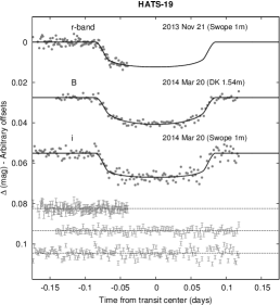
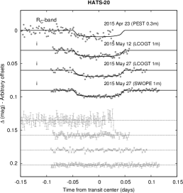
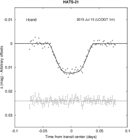
Figure 2.— Unbinned transit follow-up light curves for HATS-19 (left), HATS-20 (middle), and HATS-21 (right). The light curves have been corrected for quadratic trends in time fitted simultaneously with the transit model. The dates of the events, filters and instruments used are indicated. Light curves following the first are displaced vertically for clarity. Our best fit from the global modeling described in § 3.4 is shown by the solid lines. The residuals from the best-fit model are shown below in the same order as the original light curves. The error bars represent the photon and background shot noise, plus the readout noise.

High quality photometric observations with larger telescopes than the HATSouth instruments were obtained for the three candidates to constrain transit parameters and refine transit ephemerides. We briefly describe these observations below. Table 1 lists the various telescopes, instruments, filters, and observing parameters. Figure 2 shows all follow-up light curves for HATS-19, -20, and -21 along with transit model fits (discussed further in §  3.4). Table 2.2.2 lists all photometric observations of these three exoplanet candidates, including the initial HATSouth light curves as well as the follow up observations.

HATS-19 was observed with the Swope 1-m telescope and the SITe3 camera on 2013 November 21 (Sloan $r$; ingress event) and 2014 March 20 (Sloan $i$; full transit). Aperture photometry was performed on the frames following the procedure in Deeg & Doyle (2001) and Rabus et al. (2016), and differential magnitude light curves were obtained. Another full transit event for HATS-19 was observed using the Danish 1.54-m telescope, the DFOSC camera, and the $B$ filter, on 2015 March 20. This observation was carried out with the telescope defocused to obtain high photometric precision ($\sim 1.2$ mmag per point), and frames were reduced following the procedure described above. All three follow-up observations showed no variation in transit depth between the different filters used, greatly improving the likelihood that this transit candidate is not affected by blending with a foreground/background eclipsing binary system.

A transit ingress event for HATS-20 was observed by the 0.3-m Perth Exoplanet Survey Telescope (PEST) on 2015 April 23 using a Cousins-$R$ filter. These observations were reduced to light curves following Zhou et al. (2014b). After refining ephemerides based on this light curve, a nearly full-transit event was observed by the 1-m telescope of the Las Cumbres Observatory Global Telescope network (LCOGT; Brown et al. 2013) at the South African Astronomical Observatory (SAAO) with the SBIG camera and the Sloan $i$ filter on 2015 May 12. Another LCOGT observation of the full transit event took place on 2015 May 27 using the 1-m telescope at Cerro Tololo Inter-American Observatory (CTIO) and the Sinistro camera with the Sloan $i$ filter. Calibrated science frames were delivered by the LCOGT pipeline, which we then reduced to light curves following the procedures described in Bayliss et al. (2013). Finally, we covered yet another full-transit event including out-of-transit observations using the Swope 1-m telescope and the SITe3 camera with the Sloan $i$ filter. As before, all transit event depths were achromatic, increasing confidence in the planetary nature of these observed transits.

Finally, a full-transit event for HATS-21 was observed using the LCOGT 1-m telescope at SAAO and the SBIG camera with the Sloan $i$ filter on 2015 July 15. Due to the relatively deep transit ($\sim 10$ mmag), the ephemerides for this target were well-constrained by the HATSouth light curve itself, thus a single follow-up light curve was sufficient to characterize this candidate’s transit parameters. These observations were reduced in a similar manner to those obtained for HATS-20.

Table 3 Light curve data for HATS-19, HATS-20, and HATS-21.

Object	BJD	Mag	$\sigma_{\rm Mag}$	Mag(orig)	Filter	Instrument
	(2,400,000$+$)
HATS-19	$56045.41332$	$-0.00045$	$0.00431$	$\cdots$	$r$	HS
HATS-19	$55976.86851$	$-0.00197$	$0.00426$	$\cdots$	$r$	HS
HATS-19	$56022.56757$	$-0.00323$	$0.00465$	$\cdots$	$r$	HS
HATS-19	$56017.99833$	$0.00750$	$0.00392$	$\cdots$	$r$	HS
HATS-19	$56086.54423$	$0.00190$	$0.00499$	$\cdots$	$r$	HS
HATS-19	$56068.26668$	$-0.00722$	$0.00416$	$\cdots$	$r$	HS
HATS-19	$56018.00219$	$-0.00090$	$0.00403$	$\cdots$	$r$	HS
HATS-19	$56086.54798$	$-0.00375$	$0.00447$	$\cdots$	$r$	HS
HATS-19	$56022.57275$	$0.01002$	$0.00468$	$\cdots$	$r$	HS
HATS-19	$56068.27017$	$-0.01594$	$0.00415$	$\cdots$	$r$	HS

Note. — This table is available in a machine-readable form in the online journal. A portion is shown here for guidance regarding its form and content.

2.2.3 Imaging to rule out close companions

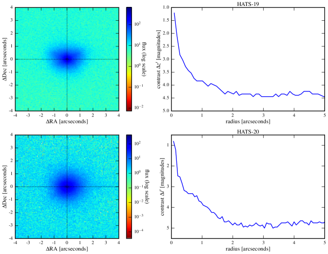
Figure 3.— Upper-left: Combined $z^{\prime}$-band frame from the AstraLux Sur lucky-imaging camera observation of HATS-19, showing no detected companions within 5 arcseconds of the target. The slightly elongated PSF is a known instrumental effect and was confirmed by observing other stars in the field. Upper-right: 5$\sigma$ detection contrast curve for HATS-19 obtained from the AstraLux combined frame. Lower-left: Combined $i^{\prime}$-band frame from the AstraLux Sur lucky-imaging camera observation of HATS-20, showing no detected companions within 5 arcseconds of the target. Lower-right: 5$\sigma$ detection contrast curve for HATS-20 obtained from the AstraLux combined frame.

Close companions to potential planet host stars can be a significant source of extra light if they remain unresolved in photometric observations of the target systems. These companion stars may in turn be unresolved multiple star systems on their own. A close-by eclipsing binary system may produce a diluted eclipse signal that mimics the characteristic depth and shape of a planetary transit across the face of the original target star. Photometric follow-up of transit candidates, therefore, should include high-resolution imaging of the target stars to rule out the possibility of a false-positive detection by the initial survey (which generally has very wide-field low angular-resolution images). For the HATSouth survey, in addition to careful inspection of follow-up images, we started observing some of our transit candidates with the AstraLux Sur lucky-imaging instrument (Hippler et al., 2009) on the ESO New Technology Telescope (NTT) at La Silla Observatory in 2015.

We observed HATS-19 on 2015 December 22 with AstraLux Sur and obtained $10^{4}$ frames with an exposure time of 70 milliseconds each in the SDSS $z^{\prime}$ filter. Similarly, HATS-20 was observed on 2015 December 28 with the AstraLux Sur instrument; we obtained $10^{4}$ frames with an exposure time of 30 milliseconds each in the SDSS $i^{\prime}$ filter. These observations were reduced following the procedure in Hormuth et al. (2008); the frames with the best 10% of the measured Strehl ratio were selected and combined into a single frame that is oversampled using a drizzle process resulting in a final pixel scale of $\sim 23.7$ milliarcseconds (mas) pixel^-1. No companions around HATS-19 or HATS-20 are detected by inspecting this final image for both targets (see upper-left panel of Figure 3 for HATS-19, and lower-left panel for HATS-20).

We obtain 5$\sigma$ detection contrast curves for HATS-19 and -20 following the procedure in Espinoza et al. (2016) and the accompanying code. We first fit for the point-spread-function (PSF) of the target, then subtract this from the image. On the residual image, we then place simulated sources with PSFs of the derived full-width at half-maximum (FWHM) of the original star and scaled fluxes corresponding to magnitude contrasts of $\Delta z^{\prime}=0$ to 10 mag at various positions on the image around the location of the target star. Finally, we attempt to recover these simulated sources, requiring that any detection be 5$\sigma$ above the background. In this way, we generate a contrast curve placing upper limits on the brightness of any close companions. We derived an effective FWHM of the PSF of the HATS-19 observation of $4.84\pm 0.35$ pixels, which corresponds to $111\pm 8$ mas. The obtained 5$\sigma$ contrast curve following this procedure is shown in the upper-right panel of Figure 3. Similarly, we derived an effective FWHM of the PSF of the HATS-20 observation of $3.39\pm 0.33$ pixels, which corresponds to $78\pm 8$ mas. The obtained 5$\sigma$ contrast curve for HATS-20 following this procedure is shown in the lower-right panel of Figure 3.

2.2.4 Precise radial velocity measurements

We observed HATS-19, -20, and -21 with high-resolution spectrographs to obtain precise measurements of their RVs and stellar parameters, and thus constrain the orbits and the fundamental properties of the planetary companions to these stars. These observations are summarized in Table 2. We briefly discuss each target’s observations below.

HATS-19 was observed extensively using three high-precision RV instruments. During 2014 March 11–16, we observed this target using the Coralie instrument on the 1.2-m Euler telescope at the European Southern Observatory (ESO) at La Silla. Coralie is a high resolution echelle spectrograph with $R=60000$. We obtained six spectra of HATS-19 during this observation run; these were reduced following the procedures laid out in Jordán et al. (2014). Twelve more spectra were obtained for HATS-19 during observing runs taking place in June 2014—Feb 2015 with the FEROS spectrograph (Kaufer & Pasquini 1998; $R=48000$) on the ESO/MPG 2.2-m telescope at La Silla. These were reduced using the Coralie pipeline described in Jordán et al. (2014) adapted for use with FEROS data. Finally, we obtained twelve more spectra using the Carnegie Planet Finder Spectrograph (PFS; Crane et al. 2010; $R=76000$) on the Magellan-II 6.5-m telescope at LCO. These spectra were obtained during observing runs in December 2014—February 2015, and reduced following Butler et al. (1996).

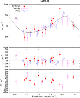
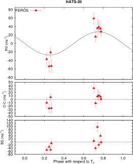
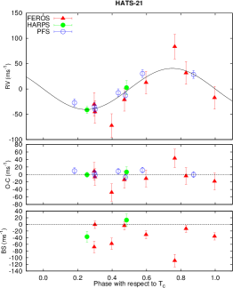
Figure 4.— Phased high-precision RV measurements for HATS-19 (left), HATS-20 (middle), and HATS-21 (right). The instruments used are labelled in the plots. For HATS-19: two observations marked with an X were obtained (partially) in transit and have been excluded from the analysis. In each case we show three panels. The top panel shows the phased measurements together with our best-fit circular-orbit model (see Table 5) for each system. Zero-phase corresponds to the time of mid-transit. The center-of-mass velocity has been subtracted. The second panel shows the velocity $O\!-\!C$ residuals from the best fit. The error bars include the jitter terms listed in Table 5 added in quadrature to the formal errors for each instrument. The third panel shows the bisector spans (BS). Note the different vertical scales of the panels.

We obtained ten spectra for HATS-20 using the FEROS instrument on the ESO/MPG 2.2-m telescope at La Silla over the period of June—July 2015. These were reduced using the procedure outlined previously. In addition, we observed this target using the High Accuracy Radial Velocity Planet Searcher instrument (HARPS; Mayor et al. 2003; $R=115000$) on the ESO 3.6-m telescope at La Silla during an observing run on 2015 April 6—8, obtaining three more spectra. These observations were reduced using the calibration pipeline provided by the instrument facility. These spectra resulted in unreliable RV measurements due to low S/N and significant sky contamination, thus were not suitable for detection of low-amplitude radial velocity variations induced by Saturn-mass companions. These were were not used for the subsequent analysis of the system.

Finally, for HATS-21, we obtained seven PFS/Magellan-II spectra during June—July 2015 and eight FEROS/MPG 2.2-m spectra during July—August 2015. These were reduced using the procedures outlined above to obtain precise RV estimates. In addition to these measurements, we also observed this target with HARPS/ESO 3.6-m during April—September 2015 (three spectra obtained) and Coralie/Euler 1.2-m during June—September 2015 (three more spectra obtained). One HARPS observation and all three Coralie observations turned out to suffer from low S/N and sky contamination; these were excluded from any further analysis.

Radial velocity curves phased with the determined orbital periods for HATS-19b, -20b, and -21b are shown in Figure 4, along with the associated bisector spans (BS) measured over the orbital phases. Table 4 lists all the measured radial velocities and bisector spans for each of three targets.

For HATS-19 and HATS-20, there is a hint that the bisector spans vary in phase with the orbital ephemeris. To check for possible correlations between the radial velocities and bisector spans, we calculated the Pearson correlation coefficient for these quantities. The bootstrap sampling derived 95%-confidence intervals for the correlation coefficient are [-0.75, -0.05], [0.22, 0.81], and [-0.77, 0.69] for HATS-19, HATS-20, and HATS-21 respectively. There is a weak correlation seen between the RVs and BS values for HATS-19 and HATS-20 (Figure 5), therefore detailed photometric blend modeling is required to rule out the possibility that these planetary RV signals are false-positives. We discuss this effort in § 3.3, where we also discuss likely explanations for the correlation.

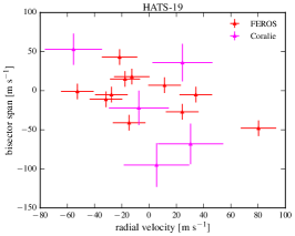
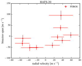
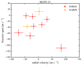
Figure 5.— Bisector-span and radial velocity correlation plots for HATS-19 (left), HATS-20 (middle), and HATS-21 (right). The instruments used are labeled in the plots. The center of mass radial velocities have been subtracted as in Figure 4.

3. Analysis

3.1. Stellar parameters for the planet hosts

Initial estimates of spectroscopic stellar parameters for HATS-19, HATS-20, and HATS-21 are obtained from the WiFeS $R=3000$ reconnaissance spectra. More reliable estimates of these parameters are obtained using the Zonal Atmospherical Stellar Parameter Estimator (ZASPE; Brahm et al. 2016, in prep) method outlined in Brahm et al. (2015) and Brahm et al. (2016). Briefly: the $\chi^{2}$ difference between the median-combined observed spectra from the FEROS instrument and synthetic spectra, generated using the SPECTRUM code (Gray, 1999) and model atmospheres from Castelli & Kurucz (2004), is minimized over a grid to obtain estimates of $T_{\rm eff}$, log $g$, [Fe/H], and $v\sin i$. Measurements of these stellar parameters obtained from a run of ZASPE are combined with constraints on the stellar mean density $\rho_{\star}$ obtained from the transit light curves (following Sozzetti et al. 2007) and orbital parameters obtained from the RV measurements during the global modeling of the data (§ 3.4).

The physical parameters $R_{\star}$, $M_{\star}$ and stellar age, are determined by comparing $T_{\rm eff\star}$, $\rm[Fe/H]$, and $\rho_{\star}$ to Yonsei-Yale (Y²; Yi et al. 2001) stellar evolution models. This results in a more precise determination of log $g_{\star}$. The log $g_{\star}$ is then held fixed and another iteration of ZASPE and comparison to ${\rm Y}^{2}$ models performed to determine the final stellar parameters. See Figure 6 for comparisons between the resulting estimates of T_eff⋆ and $\rho_{\star}$ for HATS-19, HATS-20, and HATS-21 and the model isochrones. We derive distances to each of the systems by comparing the measured magnitudes to those predicted by the Y² models in several broadband filters, assuming a $R_{V}=3.1$ extinction law from Cardelli et al. (1989). All adopted parameters, including derived stellar radii, masses, ages, and distances are detailed in Table 4.

Figure 6.— Model isochrones from Yi et al. (2001) for the measured metallicities of HATS-19 (left), HATS-20 (middle), and HATS-21 (right). We show models for ages of 0.2 Gyr and 1.0 to 14.0 Gyr in 1.0 Gyr increments (ages increasing from left to right). The adopted values of T_eff⋆ and $\rho_{\star}$ are shown together with their 1$\sigma$ and 2$\sigma$ confidence ellipsoids. The initial values of T_eff⋆ and $\rho_{\star}$ from the first iteration of ZASPE and light curve/radial velocity analyses are represented with a triangle.

HATS-19 is found to be an early G-dwarf (spectral type G0V; based on tabulations by Pecaut & Mamajek 2013 and Covey et al. 2007) with a mass of $1.303\pm 0.083$ $M_{\sun}$, radius of $1.75\pm 0.25$ $R_{\sun}$, and log $g_{\star}=4.07\pm 0.10$. The stellar effective temperature $T_{\rm eff}$ measured is $5896\pm 77$ K, the measured metallicity $\rm[Fe/H]=0.240\pm 0.050$ dex. The star is near the end of its main-sequence lifetime; its derived age is $3.94_{-0.50}^{+0.96}$ Gyr and its estimated distance is $780\pm 110$ pc.

HATS-20 is a late G dwarf (G9V) with estimated mass of $0.910\pm 0.026$ $M_{\sun}$, radius of $0.892_{-0.040}^{+0.057}$ $R_{\sun}$, and log $g_{\star}=4.497\pm 0.052$. The star has $T_{\rm eff}=5406\pm 49$ K and $\rm[Fe/H]=0.030\pm 0.050$ dex. The star is $6.4\pm 3.4$ Gyr old, and is at an estimated distance of $454_{-22}^{+30}$ pc.

Finally, HATS-21 is a mid G-dwarf star (G4V), with a measured mass of $1.080\pm 0.026$ $M_{\sun}$ and an estimated radius of $1.021_{-0.036}^{+0.089}$ $R_{\sun}$. The effective temperature is measured to be $T_{\rm eff}=5695\pm 67$ K, $\rm[Fe/H]=0.300\pm 0.040$ dex, and log $g_{\star}=4.453\pm 0.055$. The star is $2.3\pm 1.7$ Gyr old, and is at an estimated distance of $286_{-12}^{+24}$ pc.

3.2. Rotation of the host stars

We checked for signatures of stellar rotation in the HATSouth light curves for HATS-19, HATS-20, and HATS-21 by looking for sinusoidal modulation caused by star spots rotating through the line of sight. We checked for photometric variability in the EPD de-trended light curves as well as the TFA de-trended light curves. We checked both because the non-reconstructive TFA procedure is known to suppress some light curve modulation that may be astrophysical in nature. The planetary transits were masked, and we searched for any remaining periodic signals using the Generalized Lomb Scargle periodogram (Zechmeister & Kürster, 2009). No significant peaks were found in periodograms computed using the EPD and TFA light curves for any of the objects. We note that the target stars appear to be quiet slow-rotating G stars based on the lack of photometric variability, the relatively small observed radial velocity jitter, and the long estimated stellar rotation periods from the spectroscopic measured values of $v\sin i$: 18.5, 29.9, and 19.6 days for HATS-19, -20, and -21 respectively.

Table 4 Stellar parameters for HATS-19, HATS-20, and HATS-21.

	HATS-19	HATS-20	HATS-21
Parameter	Value	Value	Value	Source
Astrometric properties and cross-identifications
2MASS-ID	2MASS J09493761-3313065	2MASS J13123190-4535259	2MASS J18404426-5827332
GSC-ID	GSC 7172-01459	GSC 8247-02184	GSC 8770-00400
R.A. (J2000)	$09^{\mathrm{h}}49^{\mathrm{m}}37.63{\mathrm{s}}$	$13^{\mathrm{h}}12^{\mathrm{m}}32.04{\mathrm{s}}$	$18^{\mathrm{h}}40^{\mathrm{m}}44.40{\mathrm{s}}$	2MASS
Dec. (J2000)	$-33{\arcdeg}13{\arcmin}06.6{\arcsec}$	$-45{\arcdeg}35{\arcmin}26.0{\arcsec}$	$-58{\arcdeg}27{\arcmin}33.3{\arcsec}$	2MASS
$\mu_{\rm R.A.}$ ($\rm mas\,yr^{-1}$)	$-4.6\pm 1.3$	$-15.2\pm 1.8$	$-26.1\pm 1.7$	UCAC4
$\mu_{\rm Dec.}$ ($\rm mas\,yr^{-1}$)	$2.0\pm 1.3$	$-3.8\pm 1.8$	$-29.4\pm 1.7$	UCAC4
Spectroscopic properties
$T_{\rm eff\star}$ (K)	$5896\pm 77$	$5406\pm 49$	$5695\pm 67$	ZASPE
$\rm[Fe/H]$	$0.240\pm 0.050$	$0.030\pm 0.050$	$0.300\pm 0.040$	ZASPE
$v\sin{i}$ ($\rm km\,s^{-1}$)	$4.79\pm 0.50$	$1.51\pm 0.89$	$2.63\pm 0.55$	ZASPE
$v_{\rm mac}$ ($\rm km\,s^{-1}$)	$4.17$	$3.42$	$3.86$	Assumed
$v_{\rm mic}$ ($\rm km\,s^{-1}$)	$1.16$	$0.89$	$1.03$	Assumed
$\gamma_{\rm RV}$ ($\rm m\,s^{-1}$)	$27551.6\pm 7.2$	$22116.9\pm 4.0$	$17.3\pm 4.0$	FEROS
Photometric properties
$B$ (mag)	$13.691\pm 0.050$	$14.581\pm 0.060$	$13.018\pm 0.010$	APASS
$V$ (mag)	$13.030\pm 0.060$	$13.765\pm 0.050$	$12.191\pm 0.020$	APASS
$g$ (mag)	$13.36\pm 0.12$	$14.126\pm 0.010$	$12.595\pm 0.010$	APASS
$r$ (mag)	$12.832\pm 0.020$	$13.478\pm 0.010$	$11.954\pm 0.010$	APASS
$i$ (mag)	$12.804\pm 0.070$	$13.317\pm 0.020$	$11.833\pm 0.040$	APASS
$J$ (mag)	$11.811\pm 0.023$	$12.351\pm 0.024$	$10.912\pm 0.020$	2MASS
$H$ (mag)	$11.553\pm 0.022$	$11.951\pm 0.022$	$10.562\pm 0.022$	2MASS
$K_{s}$ (mag)	$11.510\pm 0.019$	$11.864\pm 0.023$	$10.526\pm 0.023$	2MASS
Derived properties
$M_{\star}$ ($M_{\sun}$)	$1.303\pm 0.083$	$0.910\pm 0.026$	$1.080\pm 0.026$	Y2+$\rho_{\star}$+ZASPE
$R_{\star}$ ($R_{\sun}$)	$1.75\pm 0.25$	$0.892_{-0.040}^{+0.057}$	$1.021_{-0.036}^{+0.089}$	Y2+$\rho_{\star}$+ZASPE
$\log{g_{\star}}$ (cgs)	$4.07\pm 0.10$	$4.497\pm 0.052$	$4.453\pm 0.055$	Y2+$\rho_{\star}$+ZASPE
$\rho_{\star}$ ($\rm g\,cm^{-3}$)	$0.34_{-0.11}^{+0.15}$	$1.98\pm 0.48$	$1.55\pm 0.38$	Light curves
$\rho_{\star}$ ($\rm g\,cm^{-3}$)	$0.34\pm 0.14$	$1.81\pm 0.30$	$1.42_{-0.33}^{+0.16}$	Y2+Light curves+ZASPE
$L_{\star}$ ($L_{\sun}$)	$3.31_{-0.81}^{+1.15}$	$0.612_{-0.066}^{+0.087}$	$0.98_{-0.10}^{+0.18}$	Y2+$\rho_{\star}$+ZASPE
$M_{V}$ (mag)	$3.50\pm 0.32$	$5.44\pm 0.14$	$4.85\pm 0.17$	Y2+$\rho_{\star}$+ZASPE
$M_{K}$ (mag,ESO)	$2.05\pm 0.31$	$3.62\pm 0.12$	$3.26\pm 0.15$	Y2+$\rho_{\star}$+ZASPE
Age (Gyr)	$3.94_{-0.50}^{+0.96}$	$6.4\pm 3.4$	$2.3\pm 1.7$	Y2+$\rho_{\star}$+ZASPE
$A_{V}$ (mag)	$0.012_{-0.012}^{+0.091}$	$0.044_{-0.044}^{+0.078}$	$0.047\pm 0.049$	Y2+$\rho_{\star}$+ZASPE
Distance (pc)	$780\pm 110$0	$454_{-22}^{+30}$	$286_{-12}^{+24}$	Y2+$\rho_{\star}$+ZASPE

Note. — For each system we adopt the class of model which has the highest Bayesian evidence from among those tested. For HATS-20 and HATS-21, the adopted parameters come from a fit in which the orbit is assumed to be circular. For HATS-19, the eccentricity is allowed to vary.

3.3. Ruling out blend scenarios

We carried out an analysis following Hartman et al. (2012) to rule out the possibility that our transit detections are instead unresolved foreground/background stellar eclipsing binary systems blended with the target systems, thus masquerading as planetary transit signals in either their light curves or the radial velocity measurements. We attempt to model the available photometric data (including light curves and catalog broad-band photometric measurements) for each object as a blend between an eclipsing binary star system and a third star along the line of sight. The physical properties of the stars are constrained using the Padova isochrones (Girardi et al., 2000), while we also require that the brightest of the three stars in the blend have atmospheric parameters consistent with those measured with ZASPE for the target stars HATS-19, -20, and -21. We simulate composite cross-correlation functions (CCFs) and use them to predict radial velocity (RV) signals and bisector spans (BS) for each blend scenario considered.

For all three objects, we find that blend models that cannot be rejected with at least 4$\sigma$ confidence based on the photometry alone would have produced RV and/or BS variations in excess of 1 $\rm km\,s^{-1}$, or would have been easily identified as having composite CCFs. The source of the observed BS–RV correlations remains unclear. The small radial velocity jitter measured for all three systems, coupled with no photometric detection of stellar rotation, points to low levels of stellar activity, likely ruling it out as the cause. Alternatively, any remaining unsubtracted signal from the sky background inside the spectroscopic aperture might lead to small variations in BS and RVs that coincidentally end up being correlated. Radial velocity follow-up observing runs tend to be clustered in time; the effective radial velocity signal of the scattered moonlight is similar for many of the measurements, so it is not uncommon for this effect to result in BS–RV correlations (Hartman et al., 2009). We are especially sensitive to these small signals due to the low masses and thus smaller radial velocity amplitudes of these Saturn-mass transit candidates.

Based on our blend analysis, we conclude that all three objects are indeed transiting planet systems. We cannot, however, exclude the possibility that one or more of these objects is an unresolved binary stellar system with one component hosting a short period transiting planet. The presence of a still unresolved binary star companion to either HATS-19 or HATS-20, despite the null results from lucky imaging observations presented in § 2.2.3, could also explain the slight BS–RV correlations observed for these systems. For the remainder of the paper we assume that these are all single stars with transiting planets, but we note that the radii, and potentially the masses, of the planets would be larger than what we infer here if subsequent observations reveal binary star companions.

3.4. Modeling of the data and resulting planet parameters

We modeled the HATSouth photometry, the follow-up photometry, and the high-precision RV measurements following Pál et al. (2008); Bakos et al. (2010); Hartman et al. (2012). We fit Mandel & Agol (2002) transit models to the light curves, allowing for a dilution of the HATSouth transit depth as a result of blending from neighboring stars and over-correction by the trend-filtering method. To correct for systematic errors in the follow-up light curves, we include in our model for each event a quadratic trend in time, and linear trends with up to three parameters describing the shape of the instrument point-spread-function (PSF). We fit Keplerian orbits to the RV curves allowing the zero-point for each instrument to vary independently in the fit, and allowing for RV jitter which we we also vary as a free parameter for each instrument. We used a Differential Evolution Markov Chain Monte Carlo procedure (ter Braak, 2006; Eastman et al., 2013) to explore the fitness landscape and to determine the posterior distribution of the parameters. We fit both fixed circular orbits and free-eccentricity models to the data for all three systems, and then used the method of Weinberg et al. (2013) to estimate the Bayesian evidence for each scenario. The final resulting parameters for each system are listed in Table 5, and we discuss each exoplanet briefly below.

We find that for HATS-19b, the free-eccentricity model has the higher Bayesian evidence (it is 500 times greater), and that this system has a significant non-zero eccentricity of $e=0.30\pm 0.10$. HATS-19b is more massive than Saturn, with estimated planetary mass $M_{p}=0.312\pm 0.050$ $M_{\rm J}$, a rather-inflated planetary radius $R_{p}=1.258_{-0.058}^{+0.107}$ $R_{\rm J}$, and a density $\rho_{p}=0.184_{-0.039}^{+0.052}$ $\rm g\,cm^{-3}$. The planet’s equilibrium surface temperature $T_{\rm eq}$ (averaged over the orbit, assuming zero albedo and full redistribution of heat in the planet’s atmosphere) is $1570\pm 110$ K.

For HATS-20b, the fixed circular orbit model has Bayesian evidence $3$ times greater than a free-eccentricity model, with a 95%-confidence upper limit on the eccentricity of $e<0.501$. This planet is less massive than Saturn, with $M_{p}=0.273\pm 0.035$ $M_{\rm J}$, and a measured planetary radius $R_{p}$ of $0.776\pm 0.055$ $R_{\rm J}$. HATS-20b has a density comparable to that of Saturn itself, with $\rho_{p}=0.73\pm 0.18$ $\rm g\,cm^{-3}$, despite being in close orbit around the host star (the planet’s equilibrium surface temperature $T_{\rm eq}$ is $1147\pm 36$ K).

Finally, for HATS-21b, the fixed circular orbit model has Bayesian evidence 120000 times that of an eccentric orbit model and a 95%-confidence upper limit on the eccentricity of $e<0.149$. This planet is slightly more massive than Saturn, with $M_{p}=0.332_{-0.030}^{+0.040}$ $M_{\rm J}$, an inflated planetary radius $R_{p}=1.123_{-0.054}^{+0.147}$ $R_{\rm J}$, and a density $\rho_{p}=0.290_{-0.086}^{+0.063}$ $\rm g\,cm^{-3}$. Its equilibrium surface temperature $T_{\rm eq}$ is $1284_{-31}^{+55}$ K.

Table 5Orbital and planetary parameters for HATS-19b, HATS-20b and HATS-21b

	HATS-19b	HATS-20b	HATS-21b
Parameter	Value	Value	Value
Light curve parameters
$P$ (days)	$4.569673\pm 0.000010$	$3.7992969\pm 0.0000079$	$3.5543973\pm 0.0000058$
$T_{c}$ (${\rm BJD}$)	$2456660.03375\pm 0.00059$	$2457121.16516\pm 0.00055$	$2457109.22538\pm 0.00057$
$T_{12}$ (days)	$0.1666\pm 0.0020$	$0.1022\pm 0.0016$	$0.0824\pm 0.0026$
$T_{12}=T_{34}$ (days)	$0.0164\pm 0.0016$	$0.0117\pm 0.0016$	$0.027\pm 0.034$
$a/R_{\star}$	$7.24\pm 0.90$	$11.14\pm 0.63$	$9.84_{-0.83}^{+0.35}$
$\zeta/R_{\star}$	$13.32\pm 0.11$0	$22.01\pm 0.24$0	$33.41_{-0.84}^{+1.52}$0
$R_{p}/R_{\star}$	$0.0976\pm 0.0021$	$0.0898\pm 0.0022$	$0.113\pm 0.011$
$b^{2}$	$0.105_{-0.068}^{+0.080}$	$0.303_{-0.077}^{+0.085}$	$0.728_{-0.024}^{+0.059}$
$b\equiv a\cos i/R_{\star}$	$0.32_{-0.13}^{+0.11}$	$0.551_{-0.075}^{+0.072}$	$0.853_{-0.014}^{+0.034}$
$i$ (deg)	$86.6\pm 1.7$0	$87.16\pm 0.54$0	$85.04_{-0.65}^{+0.23}$0
HATSouth blend factors
Blend factor 1	$0.868\pm 0.052$	$0.62\pm 0.17$	$0.757\pm 0.070$
Blend factor 2	$0.857\pm 0.047$	$0.876\pm 0.074$	$0.741\pm 0.059$
Limb-darkening coefficients
$c_{1},B$ (linear term)	$0.6289$	$\cdots$	$\cdots$
$c_{2},B$ (quadratic term)	$0.1892$	$\cdots$	$\cdots$
$c_{1},R$	$\cdots$	$0.4077$	$\cdots$
$c_{2},R$	$\cdots$	$0.2811$	$\cdots$
$c_{1},r$	$0.3468$	$0.4366$	$0.3952$
$c_{2},r$	$0.3369$	$0.2753$	$0.3072$
$c_{1},i$	$0.2566$	$0.3320$	$0.2962$
$c_{2},i$	$0.3437$	$0.2933$	$0.3225$
RV parameters
$K$ ($\rm m\,s^{-1}$)	$46.1\pm 8.0$00	$37.9\pm 4.8$00	$41.6\pm 4.3$00
$e$	$0.30\pm 0.10$	$<0.501$	$<0.149$
$\omega$ (deg)	$44\pm 50$	$\cdots$	$\cdots$
$\sqrt{e}\cos\omega$	$0.39\pm 0.13$	$\cdots$	$\cdots$
$\sqrt{e}\sin\omega$	$0.37\pm 0.16$	$\cdots$	$\cdots$
$e\cos\omega$	$0.209\pm 0.084$	$\cdots$	$\cdots$
$e\sin\omega$	$0.20\pm 0.11$	$\cdots$	$\cdots$
RV jitter FEROS ($\rm m\,s^{-1}$)	$15.6\pm 6.2$	$<8.6$	$20.0\pm 10.0$
RV jitter HARPS ($\rm m\,s^{-1}$)	$\cdots$	$\cdots$	$<0.4$
RV jitter Coralie ($\rm m\,s^{-1}$)	$<13.2$	$\cdots$	$\cdots$
RV jitter PFS ($\rm m\,s^{-1}$)	$11.4\pm 3.6$	$\cdots$	$7.3\pm 2.9$
Planetary parameters
$M_{p}$ ($M_{\rm J}$)	$0.427\pm 0.071$	$0.273\pm 0.035$	$0.332_{-0.030}^{+0.040}$
$R_{p}$ ($R_{\rm J}$)	$1.66_{-0.21}^{+0.27}$	$0.776\pm 0.055$	$1.123_{-0.054}^{+0.147}$
$C(M_{p},R_{p})$	$0.55$	$-0.03$	$-0.03$
$\rho_{p}$ ($\rm g\,cm^{-3}$)	$0.116\pm 0.042$	$0.73\pm 0.18$	$0.290_{-0.086}^{+0.063}$
$\log g_{p}$ (cgs)	$2.58\pm 0.10$	$3.050\pm 0.084$	$2.811_{-0.108}^{+0.068}$
$a$ (AU)	$0.0589\pm 0.0013$	$0.04619\pm 0.00044$	$0.04676\pm 0.00038$
$T_{\rm eq}$ (K)	$1570\pm 110$	$1147\pm 36$	$1284_{-31}^{+55}$
$\Theta$	$0.0231\pm 0.0036$	$0.0355\pm 0.0050$	$0.0253\pm 0.0041$
$\log_{10}\langle F\rangle$ (cgs)	$9.14\pm 0.12$	$8.592\pm 0.054$	$8.787_{-0.043}^{+0.072}$

Note. — For each system we adopt the class of model which has the highest Bayesian evidence from among those tested. For HATS-20b and HATS-21b the adopted parameters come from a fit in which the orbit is assumed to be circular. For HATS-19b the eccentricity is allowed to vary.

4. Discussion

We plot the derived masses and radii for HATS-19b, -20b, and -21b in Figure 7, along with 252 other transiting giant exoplanets from the literature (taken from exoplanets.org on 2016 April 12) with measured masses $M_{\rm p}>0.1\ M_{\rm J}$. HATS-19b is immediately seen as an outlier due to its highly inflated radius compared to the theoretical mass-radius relations from Fortney et al. (2007). Other highly-inflated Saturn-mass planets with radii comparable to HATS-19b include WASP-31b (Anderson et al. 2011; $R=1.55\ R_{\rm J}$), WASP-94 A b (Neveu-VanMalle et al. 2014; $R=1.72\ R_{\rm J}$), and Kepler-12b (Fortney et al. 2011; $R=1.70\ R_{\rm J}$). These planets orbit host stars with ${\rm[Fe/H]}=-0.20$, $+0.26$, and $+0.07$, respectively, while HATS-19b has a host star with ${\rm[Fe/H]}=+0.24$. The highly inflated radius observed for HATS-19b despite its host star’s enhanced metallicity and increased heavy element fraction may be explained by the combination of kinetic heating in the planet interior (Guillot & Showman, 2002), opacity-induced energy transport inefficiencies (Burrows et al., 2007), and additional energy input by tidal heating due to the planet’s eccentric orbit (Jackson et al., 2008).

HATS-20b is a dense planet orbiting an older star with nearly-Solar metallicity. HATS-20b’s position in the mass-radius plane despite being in close orbit around its host star is likely to be a result of a large inferred core mass ($>25\ M_{\oplus}$) combined with its relatively low level of insolation receiving much less energy deposited into its atmosphere, and perhaps thermal contraction over the long main-sequence life-time of the host star.

Finally, HATS-21b is another Saturn-mass planet orbiting a star that has enhanced metallicity ${\rm[Fe/H]}=+0.30$, yet has a significantly inflated radius. Models from Fortney et al. (2007) calculated at the level of stellar irradiation expected (near 0.045 AU from the star) and an age of 1.0 Gyr appear to encompass the observed radius of the planet, but these require small core masses ($<10\ M_{\oplus}$). The small core mass, combined with the high level of insolation may serve to inflate the planetary radius to the observed value.

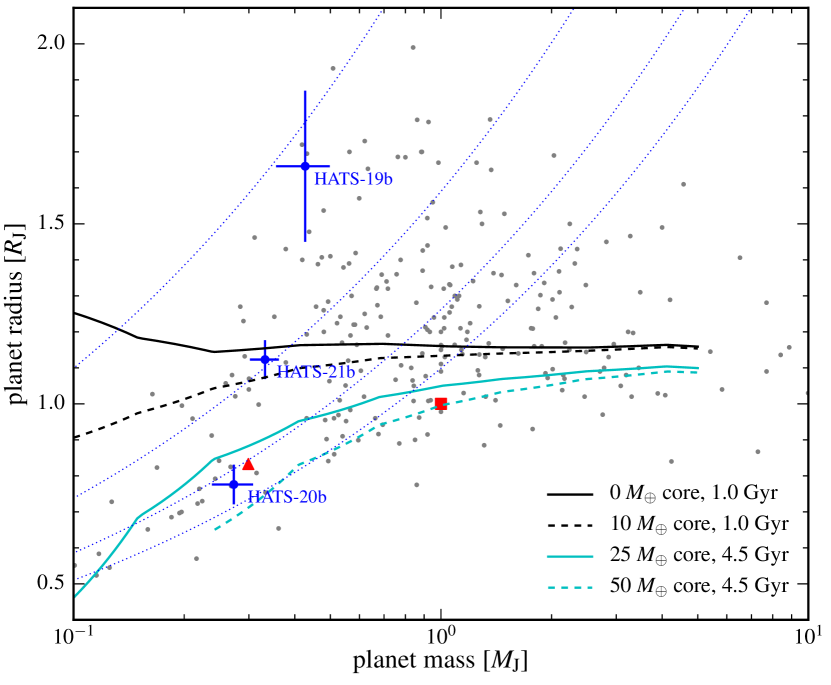
Figure 7.— The planet mass in $M_{\rm J}$ and planet radius in $R_{\rm J}$ plotted for 252 well-characterized transiting giant exoplanets selected from exoplanets.org (see text for method; errorbars suppressed for clarity) with mass $M_{\rm p}>0.1M_{\rm J}$. In addition to this sample, HATS-19b, -20b, and -21b are shown as filled blue circles. The lines depict the mass-radius relations from Fortney et al. (2007), for irradiated planets at 0.045 AU from the host star at 1.0 Gyr (black lines) and 4.5 Gyr (cyan lines). For the 1.0 Gyr relations, solid lines depict core masses of 0 $M_{\oplus}$ and dashed lines depict core masses of 10 $M_{\oplus}$. For the 4.5 Gyr relations, the solid lines depict core masses of 25 $M_{\oplus}$ and dashed lines depict core masses of 50 $M_{\oplus}$. The position of Saturn in this mass-radius plane is shown as the filled red triangle, while that of Jupiter is shown as the filled red square. The blue dotted iso-density lines are for $\rho=0.10$, $0.33$, $0.66$, and ${1.0\ \rm g\ cm^{-3}}$ from left to right.

Relations between various physical parameters and the observed giant planet radii have been investigated by Laughlin et al. (2011), Béky et al. (2011), Enoch et al. (2012, hereafter E12), and Zhou et al. (2014a), among others. In particular, E12 fit empirical relations to the radii of Saturn- and Jupiter-mass giant planets as functions of stellar irradiation parameterized by $T_{\rm eq}$, planet host metallicity $\rm[Fe/H]$, planet mass $M_{p}$, orbital semi-major axis $a$, and the tidal heating rate $H$. Significant correlations were found between planet radius and planet equilibrium temperature $T_{\rm eq}$, as well as between planet radius and host star metallicity $\rm[Fe/H]$. Figure 8 summarizes the relations between the planet radius $R_{\rm p}$, planetary equilibrium temperature $T_{\rm eq}$, and stellar metallicity $\rm[Fe/H]$ for 204 irradiated transiting giant exoplanets with measured masses $M_{\rm p}>0.1M_{\rm J}$ and periods $P<10$ days taken from exoplanets.org (accessed on 2016 April 12) plus HATS-19b, -20b, and -21b. In addition to these criteria, the host stars for these selected planets were required to have measured values of metallicity and effective temperature. There is a significant strong positive correlation seen between the planetary radius and equilibrium temperature, with a bootstrap 95% confidence interval of the correlation coefficient of [+0.52, +0.70]. On the other hand, there is only a weak negative correlation seen between the planetary radius and stellar metallicity with a bootstrap 95%-confidence interval of the correlation coefficient of [-0.28, -0.02], but it still appears statistically significant. Both results are in line with the conclusions in E12.

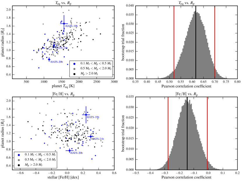
Figure 8.— Upper-left: The planet equilibrium temperature $T_{\rm eq}$ and planet radius $R_{\rm p}$ plotted for 205 transiting exoplanets selected in the same way as for Figure 7, but restricted to orbital periods $P<10$ days to select irradiated planets. Blue filled circles represent hot-Saturns ($0.1<M_{\rm p}<0.5$ $M_{J}$), grey filled circles represent hot-Jupiters planets ($0.5<M_{\rm p}<2.0$ $M_{J}$), and black filled circles represent high-mass planets ($M_{\rm p}>2.0$ $M_{J}$). HATS-19b, -20b, and -21b are shown as filled blue squares. Upper-right: The median Pearson correlation coefficient (black line) for the relation between $T_{\rm eq}$ and $R_{\rm p}$ for all planets in this sample determined after $10^{5}$ bootstrap trials along with its 95% confidence limits (red lines). Lower-left: The stellar metallicity ${\rm[Fe/H]}$ and planet radius $R_{\rm p}$ for the same sample. HATS-19b, -20b, and -21b are shown as filled blue squares. Lower-right: The median Pearson correlation coefficient (black line) for the relation between ${\rm[Fe/H]}$ and $R_{\rm p}$ of all planets in this sample determined after $10^{5}$ bootstrap trials along with its 95% confidence limits (red lines).

Characterizing the empirical relations of planetary and host star parameters to the observed planet radii may help distinguish between various proposed models of the input, internal transport, and loss of energy from planetary atmospheres, and may explain the observed radius distributions. We investigate the relative importance of these parameters by fitting a model relating them to the observed planet radius using regression carried out with Random Forests (Breiman, 2001). Random forest regression does not require explicit functional forms for the dependence between model parameters and the explained variable. It also includes a way to determine the relative importance of the regression model parameters. We used the implementation of this method in the Python scikit-learn library (Pedregosa et al., 2011); see Appendix A for details.

Using the random forest regression method, we fit the following model for the observed planetary radius $R_{p}$, which is described as a function of the predictor variables $T_{\rm eq}$ (the equilibrium temperature), ${\rm[Fe/H]}$ (planet host metallicity), $M_{p}$ (planet mass), $a$ (orbital semi-major axis), $e$ (orbital eccentricity), and $M_{\star}$ (planet host mass):

$$R_{p}\sim f(T_{\rm eq},{\rm[Fe/H]},M_{p},a,e,M_{\star})$$ (1)

We break up the sample of 207 irradiated giant transiting planets ($P<10$ days) that have measured values of radius, mass, semi-major axis, host metallicity, host mass, and orbital eccentricity into three sets: hot-Saturns ($0.1<M_{p}<0.5\ M_{\rm J}$; 37 members), hot-Jupiters ($0.5<M_{p}<2.0\ M_{\rm J}$; 125 members), and higher mass planets ($M_{p}>2.0\ M_{\rm J}$; 45 members). This allows us to investigate which model parameters are more important for each class of planet, and enables a comparison with E12, which used an identical scheme to break up their sample of planets and characterize relations between their physical parameters and observed planet radii.

Results of the model training and fitting process are shown in Figure 9 for each set of planets. The median absolute difference between the predicted and observed radii is 0.08, 0.06, and 0.04 $R_{\rm J}$ for Saturn-, Jupiter-, and high-mass planets respectively. The findings are broadly similar to those in E12, and are summarized below. We note that these conclusions are based on the observed sample of transiting giant exoplanets, without correcting for observational completeness. In particular, the bias towards brighter stars in the observed target population prefers main sequence stars with higher luminosity, mass, and radius, which results in a preference for transiting giant planets with larger radii that are more easily detectable. As such, the radii of all giant planet classes show a significant dependency on the planet host star mass. We assume that observational biases do not affect the correlations measured between the planetary radius and the other physical parameters. Taking these caveats into account:

• The radii of hot-Saturns appear to be largely dependent on planet mass and then on equilibrium temperature, with a small dependence on the planet host metallicity. This suggests that these planets are core-dominated (Miller & Fortney, 2011), and thus require inflation mechanisms more sensitive to heavy element content in the core, such as kinetic heating (Guillot & Showman, 2002), as opposed to mechanisms that rely on atmospheric opacity induced energy transport inefficiency (Burrows et al., 2007).

• The radii of hot-Jupiters are far more dependent on the equilibrium temperature than on either planet mass or planet host metallicity, unlike the lower mass hot-Saturns. This suggests an inflation mechanism strongly tied to the radiation incident on the planets, such as Ohmic heating (Laughlin et al., 2011; Batygin et al., 2011).

• The radii of irradiated higher mass planets appear to be largely dependent on the equilibrium temperature, with smaller dependencies on the planet mass and host metallicity of comparable magnitude. In this mass regime, the inflation mechanism may be a combination of Ohmic heating and energy transport inefficiency caused by the increasing presence of heavy elements in the envelope. Interestingly, the planet radius shows a small but significant dependence on the orbital eccentricity as well, indicating that tidal heating may play an increasing role in this mass regime.

• Eccentricity of the orbit appears to play nearly no role in determining the planet radii, except for the high mass planets. Note that the observed eccentricity in most cases is an upper limit, and is usually set to zero if not fully determined when fitting photometric and RV data to obtain planet parameters. The true eccentricity for these assumed-circular orbits may be up to 0.03 (Jackson et al., 2008); its effect on the planetary radius via tidal heating may thus be under-estimated in this sample.

Much of the uncertainty in characterizing the relations between giant planet radii and other physical parameters arises due to the small number of lower mass planets; there are only 37 Saturn-mass vs. 170 Jupiter-mass and higher-mass planets in the sample discussed in this work. A larger sample with directly measured masses, radii, and other physical parameters is required to effectively determine correlations that may distinguish between inflation mechanisms for these irradiated planets. To this end, one of the most important contributions that exoplanet transit surveys will make in the next few years will be to fill out this parameter space by discovering and characterizing with high precision populations of giant planets with masses $M_{\rm p}<1.0\ M_{\rm J}$ over a wide range in orbital semi-major axis and planet host metallicity and luminosity.

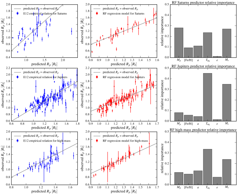
Figure 9.— Upper-left: Observed and predicted radii from the E12 relation for Saturn-mass planets ($0.1<M_{p}<0.5\ M_{\rm J}$). The gray line indicates $R_{\rm predicted}=R_{\rm observed}$. Upper-middle: Observed and predicted radii from the Random Forest regression (RF) model for Saturn-mass planets. Upper-right: Relative importance for six predictor variables used in the RF model for Saturn-mass planets. These have been normalized so that they sum to 1.0. Center-left: Observed and predicted radii from the E12 relation for Jupiter-mass planets ($0.5<M_{p}<2.0\ M_{\rm J}$). Center-middle: Observed and predicted radii from the RF model for Jupiter-mass planets. Center-right: Relative importance for six predictor variables used in the RF model for Jupiter-mass planets. Lower-left: Observed and predicted radii from the E12 relation for high-mass planets ($M_{p}>2.0\ M_{\rm J}$). Lower-middle: Observed and predicted radii from the RF model for high-mass planets. Lower-right: Relative importance for six predictor variables used in the RF model for high-mass planets.

Table 6 Relative radial velocities and bisector spans for HATS-19, HATS-20, and HATS-21.

$6823.69583$ $58.81$ $13.00$ $6.0$ $18.0$ $0.704$ FEROS $7169.57227$ $35.81$ $21.00$ $96.0$ $28.0$ $0.741$ FEROS $7171.58541$ $-53.19$ $15.00$ $-9.0$ $19.0$ $0.271$ FEROS $7188.61909$ $38.81$ $13.00$ $-19.0$ $19.0$ $0.754$ FEROS $7190.55437$ $-21.19$ $11.00$ $-51.0$ $16.0$ $0.264$ FEROS $7192.48301$ $34.81$ $12.00$ $39.0$ $17.0$ $0.771$ FEROS $7224.59573$ $-37.19$ $15.00$ $-52.0$ $20.0$ $0.224$ FEROS $7226.48662$ $15.81$ $12.00$ $-41.0$ $17.0$ $0.721$ FEROS $7228.48803$ $-54.19$ $12.00$ $-32.0$ $17.0$ $0.248$ FEROS $7230.50050$ $27.81$ $10.00$ $-3.0$ $15.0$ $0.778$ FEROS    HATS-21    $7120.79111$ $-41.40$ $7.00$ $-37.0$ $16.0$ $0.254$ HARPS $7198.72802$ $-27.23$ $2.70$  $\cdots$   $\cdots$  $0.181$ PFS $7199.78234$ $-13.02$ $2.69$  $\cdots$   $\cdots$  $0.477$ PFS $7202.69703$ $-35.23$ $2.66$  $\cdots$   $\cdots$  $0.297$ PFS $7202.70863$ $-40.48$ $2.79$  $\cdots$   $\cdots$  $0.301$ PFS $7203.69037$ $30.37$ $2.21$  $\cdots$   $\cdots$  $0.577$ PFS $7204.74545$ $28.64$ $2.29$  $\cdots$   $\cdots$  $0.874$ PFS $7206.74234$ $-7.54$ $2.25$  $\cdots$   $\cdots$  $0.435$ PFS $7224.64150$ $-21.45$ $10.00$ $-4.0$ $13.0$ $0.471$ FEROS $7227.58606$ $-45.45$ $10.00$ $-1.0$ $11.0$ $0.300$ FEROS $7228.64518$ $12.55$ $10.00$ $-31.0$ $12.0$ $0.598$ FEROS $7232.79230$ $83.55$ $14.00$ $-109.0$ $19.0$ $0.764$ FEROS $7233.61616$ $-17.45$ $10.00$ $-36.0$ $11.0$ $0.996$ FEROS $7234.68050$ $-30.45$ $12.00$ $-68.0$ $17.0$ $0.296$ FEROS $7236.57993$ $31.55$ $10.00$ $-13.0$ $11.0$ $0.830$ FEROS $7238.59579$ $-72.45$ $12.00$ $-58.0$ $17.0$ $0.397$ FEROS $7281.55714$ $2.60$ $14.00$ $13.0$ $18.0$ $0.484$ HARPS

Note. — The PFS observations of HATS-19 and HATS-21 without a BS measurement have too low S/N in the I₂-free blue spectral region to pass our quality threshold for calculating accurate BS values.

Appendix A Random forest regression

Given a set of $m$ predictors for a sample of $n$ observations of $\mathrm{Y}$, $\mathbf{X}=\{(x_{1,1}\ldots x_{m,1}),(x_{1,2}\ldots x_{m,2}),\ldots,(x_{1,n}\ldots x_{m,n})\}$, a decision tree splits $\mathbf{X}$ and the accompanying $\mathbf{Y}$ recursively until the leaf nodes are reached (with a single sample per node), or the tree construction is halted at a certain depth. For each node in the tree, a set of predictors is chosen so that a split based on a threshold applied to these predictors minimizes the “impurity” of the samples in the subsequent left and right child nodes (this is the “best” split; see Breiman et al. 1984). The “impurity” $I$ in decision trees used for regression is defined as:

$$I=\frac{n_{\mathrm{left}}}{N_{\mathrm{node}}}H_{\mathrm{left}}+\frac{n_{\mathrm{right}}}{N_{\mathrm{node}}}H_{\mathrm{right}},$$ (A1)

where $n_{\mathrm{left}}$ is the number of items after a proposed split in the left child node, $n_{\mathrm{right}}$ is the number of items after a proposed split in the right child node, and $N_{\mathrm{node}}$ is the total number of items in the current node. $H_{\mathrm{left}}$ and $H_{\mathrm{right}}$ are the variances of predicted values in the left and right child nodes, respectively:

$$H_{\mathrm{z}}=\frac{1}{N_{\mathrm{node}}}\sum_{i,\mathrm{z}\in N_{\mathrm{node}}}(y_{i,\mathrm{z}}-c_{\mathrm{node}})^{2},$$ (A2)

where z refers to either the left or right child node, and $c_{\mathrm{node}}$ is defined as:

$$c_{\mathrm{node}}=\frac{1}{N_{\mathrm{node}}}\sum_{{i}\in N_{\mathrm{node}}}y_{i}.$$ (A3)

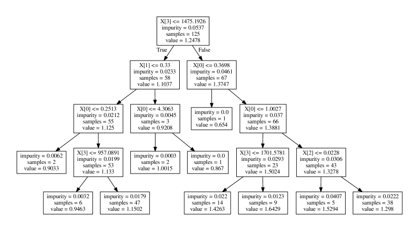
Figure 10.— The structure for a single decision tree from the random forest used to fit a regression model to the observed planet radii (“value” above) using various predictors (the vector $\mathbf{X}$ above). The “impurity” above refers to the criterion used to split the sample in the tree node at each level (see text for definition).

The prediction of an observed value is obtained by following the decision tree along these splits in the predictor values to the deepest level of the tree. The relative importance of a predictor is calculated by determining how much it contributes to reducing the “impurity” of the node samples at each level of the tree. Predictors that are used to split the nodes near the top of the tree are thus deemed more important than those that contribute to splits near the bottom of the tree. Note, however, that degeneracies between the model parameters themselves may result in calculated importances that do not reflect their true values (Grömping, 2012).

Figure 10 shows how this works for a decision tree used in regression between planet radius and several predictor variables (discussed in § 4). At the top level, the sample is split based on $X[3]$ (the equilibrium temperature in this case). The predicted value of the radius for this node is simply the mean of all radius values in the node sample. The two resulting nodes at the next level of the tree are themselves split based on $X[1]$ (metallicity) for the left node, and on $X[0]$ (planet mass) respectively. This splitting process continues until either there is only one element left in the node sample, or the construction of the tree is halted.

Decision tree regression in this way amounts to fitting sums of successive step functions based on the “best” splits for each predictor at each level of the tree. The process is non-parametric and does not rely on a prior functional form of the model. On the other hand, decision tree regression is very prone to overfitting if the tree is allowed to grow all the way to leaf nodes. In addition, small changes in the sample used to construct the tree can lead to very different trees being constructed. Ensembles of decision trees overcome these limitations, especially if different sets of predictors are chosen to split each tree. In particular, random forests (Breiman, 2001) carry out bootstrap sampling of the full set of predictors, use the chosen samples of predictors to construct decision trees, and then average the predictions of these trees to estimate the final predicted values of the observations. The final relative importance of predictors may also be calculated as the average of the determined values of predictor importance for each tree.

Practical implementations of random forest regression involve tuning of so-called hyper-parameters. These are variables associated with the construction process of the ensemble of decision trees and include: $d_{\rm max}$ (the maximum depth of each tree), $n_{\rm trees}$ (the total number of decision trees), $m_{\rm split}$ (the maximum number of predictors to consider when calculating the “best” split for a node), $s_{\rm split}$ (the minimum number of samples in a node required to consider a split), and $s_{\rm leaf}$ (the minimum number of samples required for a node to consider it a leaf node).

Optimizing these hyper-parameters results in better performance of the trained random forest regression model. This usually involves a grid-search among the parameters listed above, seeking to minimize a performance metric (in our case, the median absolute deviation of the predicted values from the observed values). In lieu of an exhaustive grid search, a random search in the hyper-parameter space may be performed, and appears to return hyper-parameter values that perform just as well (Bergstra & Bengio, 2012). The search for optimal hyper-parameters is carried out repeatedly using subsets of the training sample, training the model on one subset, validating it on the next subset, and testing it on the rest of the subsets. The whole procedure is referred to as cross-validation. In this way, the regression model with the best performance on the majority of the test subsets can be determined, and then used for all subsequent predictions.

We utilize the Python library scikit-learn (Pedregosa et al., 2011) for the entire procedure described above. The RandomForestRegressor class is used. We tune the hyper-parameters by using a random search cross-validation among the following distributions:

• $d_{\rm max}=[3,4,5,10,20,{\rm full}]$,

• $n_{\rm trees}={\rm Uniform}(100,2000)$,

• $m_{\rm split}={\rm Uniform}(1,6)$,

• $s_{\rm split}={\rm Uniform}(1,11)$,

• and $s_{\rm leaf}={\rm Uniform}(1,11)$.

We conduct a 3-fold cross-validation to optimize the model further as part of the hyper-parameter search described above. This involves breaking each sample of predictors and observations into three subsets; we train and validate the model on the first two subsets, and test it on the final subset.

As the regression models are non-parametric, no simple functional relations can be written down. Instead, we provide the trained models as Python pickles that may readily be imported, and an accompanying Jupyter notebook explaining their use at: https://github.com/waqasbhatti/hats19to21.

References

- Anderson et al. (2011) Anderson, D. R., Collier Cameron, A., Hellier, C., et al. 2011, A&A, 531, A60
- Baglin (2003) Baglin, A. 2003, Advances in Space Research, 31, 345
- Bakos et al. (2004) Bakos, G., Noyes, R. W., Kovács, G., et al. 2004, PASP, 116, 266
- Bakos et al. (2010) Bakos, G. Á., Torres, G., Pál, A., et al. 2010, ApJ, 710, 1724
- Bakos et al. (2013) Bakos, G. Á., Csubry, Z., Penev, K., et al. 2013, PASP, 125, 154
- Batygin et al. (2011) Batygin, K., Stevenson, D. J., & Bodenheimer, P. H. 2011, ApJ, 738, 1
- Bayliss et al. (2013) Bayliss, D., Zhou, G., Penev, K., et al. 2013, AJ, 146, 113
- Béky et al. (2011) Béky, B., Bakos, G. Á., Hartman, J., et al. 2011, ApJ, 734, 109
- Bergstra & Bengio (2012) Bergstra, J., & Bengio, Y. 2012, The Journal of Machine Learning Research, 13, 281
- Borucki et al. (2010) Borucki, W. J., Koch, D., Basri, G., et al. 2010, Science, 327, 977
- Brahm et al. (2015) Brahm, R., Jordán, A., Hartman, J. D., et al. 2015, AJ, 150, 33
- Brahm et al. (2016) Brahm, R., Jordán, A., Bakos, G. Á., et al. 2016, AJ, 151, 89
- Breiman (2001) Breiman, L. 2001, Machine Learning, 45, 5
- Breiman et al. (1984) Breiman, L., Friedman, J., Stone, C. J., & Olshen, R. A. 1984, Classification and regression trees (CRC press)
- Brown et al. (2013) Brown, T. M., Baliber, N., Bianco, F. B., et al. 2013, PASP, 125, 1031
- Burrows et al. (2007) Burrows, A., Hubeny, I., Budaj, J., & Hubbard, W. B. 2007, ApJ, 661, 502
- Butler et al. (1996) Butler, R. P., Marcy, G. W., Williams, E., et al. 1996, PASP, 108, 500
- Cardelli et al. (1989) Cardelli, J. A., Clayton, G. C., & Mathis, J. S. 1989, ApJ, 345, 245
- Castelli & Kurucz (2004) Castelli, F., & Kurucz, R. L. 2004, ArXiv Astrophysics e-prints
- Claret (2004) Claret, A. 2004, A&A, 428, 1001
- Covey et al. (2007) Covey, K. R., Ivezić, Ž., Schlegel, D., et al. 2007, AJ, 134, 2398
- Crane et al. (2010) Crane, J. D., Shectman, S. A., Butler, R. P., et al. 2010, in Society of Photo-Optical Instrumentation Engineers (SPIE) Conference Series, Vol. 7735, Society of Photo-Optical Instrumentation Engineers (SPIE) Conference Series
- Deeg & Doyle (2001) Deeg, H. J., & Doyle, L. R. 2001, in Third Workshop on Photometry, ed. W. J. Borucki & L. E. Lasher, 85
- Dopita et al. (2007) Dopita, M., Hart, J., McGregor, P., et al. 2007, Ap&SS, 310, 255
- Eastman et al. (2013) Eastman, J., Gaudi, B. S., & Agol, E. 2013, PASP, 125, 83
- Enoch et al. (2012) Enoch, B., Collier Cameron, A., & Horne, K. 2012, A&A, 540, A99
- Espinoza et al. (2016) Espinoza, N., Bayliss, D., Hartman, J. D., et al. 2016, ArXiv e-prints, 1606.00023
- Fortney et al. (2007) Fortney, J. J., Marley, M. S., & Barnes, J. W. 2007, ApJ, 659, 1661
- Fortney et al. (2011) Fortney, J. J., Demory, B.-O., Désert, J.-M., et al. 2011, ApJS, 197, 9
- Girardi et al. (2000) Girardi, L., Bressan, A., Bertelli, G., & Chiosi, C. 2000, A&AS, 141, 371
- Gray (1999) Gray, R. O. 1999, SPECTRUM: A stellar spectral synthesis program, Astrophysics Source Code Library
- Grömping (2012) Grömping, U. 2012, The American Statistician
- Guillot & Showman (2002) Guillot, T., & Showman, A. P. 2002, A&A, 385, 156
- Gustafsson et al. (2008) Gustafsson, B., Edvardsson, B., Eriksson, K., et al. 2008, A&A, 486, 951
- Hansen & Barman (2007) Hansen, B. M. S., & Barman, T. 2007, ApJ, 671, 861
- Hartman et al. (2009) Hartman, J. D., Bakos, G. Á., Torres, G., et al. 2009, ApJ, 706, 785
- Hartman et al. (2012) Hartman, J. D., Bakos, G. Á., Béky, B., et al. 2012, AJ, 144, 139
- Hartman et al. (2015) Hartman, J. D., Bayliss, D., Brahm, R., et al. 2015, AJ, 149, 166
- Henden et al. (2009) Henden, A. A., Welch, D. L., Terrell, D., & Levine, S. E. 2009, in American Astronomical Society Meeting Abstracts, Vol. 214, American Astronomical Society Meeting Abstracts #214, #407.02
- Hippler et al. (2009) Hippler, S., Bergfors, C., Brandner, W., et al. 2009, The Messenger, 137, 14
- Hormuth et al. (2008) Hormuth, F., Brandner, W., Hippler, S., & Henning, T. 2008, Journal of Physics: Conference Series, 131, 012051
- Jackson et al. (2008) Jackson, B., Greenberg, R., & Barnes, R. 2008, ApJ, 681, 1631
- Jordán et al. (2014) Jordán, A., Brahm, R., Bakos, G. Á., et al. 2014, AJ, 148, 29
- Kaufer & Pasquini (1998) Kaufer, A., & Pasquini, L. 1998, in Society of Photo-Optical Instrumentation Engineers (SPIE) Conference Series, Vol. 3355, Optical Astronomical Instrumentation, ed. S. D’Odorico, 844–854
- Kovács et al. (2005) Kovács, G., Bakos, G., & Noyes, R. W. 2005, MNRAS, 356, 557
- Kovács et al. (2002) Kovács, G., Zucker, S., & Mazeh, T. 2002, A&A, 391, 369
- Laughlin et al. (2011) Laughlin, G., Crismani, M., & Adams, F. C. 2011, ApJ, 729, L7
- Mandel & Agol (2002) Mandel, K., & Agol, E. 2002, ApJ, 580, L171
- Mayor et al. (2003) Mayor, M., Pepe, F., Queloz, D., et al. 2003, The Messenger, 114, 20
- Miller & Fortney (2011) Miller, N., & Fortney, J. J. 2011, ApJ, 736, L29
- Neveu-VanMalle et al. (2014) Neveu-VanMalle, M., Queloz, D., Anderson, D. R., et al. 2014, A&A, 572, A49
- Pál et al. (2008) Pál, A., Bakos, G. Á., Torres, G., et al. 2008, ApJ, 680, 1450
- Pecaut & Mamajek (2013) Pecaut, M. J., & Mamajek, E. E. 2013, ApJS, 208, 9
- Pedregosa et al. (2011) Pedregosa, F., Varoquaux, G., Gramfort, A., et al. 2011, Journal of Machine Learning Research, 12, 2825
- Penev et al. (2013) Penev, K., Bakos, G. Á., Bayliss, D., et al. 2013, AJ, 145, 5
- Pepper et al. (2007) Pepper, J., Pogge, R. W., DePoy, D. L., et al. 2007, PASP, 119, 923
- Pollacco et al. (2006) Pollacco, D. L., Skillen, I., Collier Cameron, A., et al. 2006, PASP, 118, 1407
- Rabus et al. (2016) Rabus, M., Jordán, A., Hartman, J. D., et al. 2016, ArXiv e-prints, 1603.02894
- Sozzetti et al. (2007) Sozzetti, A., Torres, G., Charbonneau, D., et al. 2007, ApJ, 664, 1190
- ter Braak (2006) ter Braak, C. J. F. 2006, Statistics and Computing, 16, 239
- Weinberg et al. (2013) Weinberg, M. D., Yoon, I., & Katz, N. 2013, ArXiv e-prints, 1301.3156
- Yi et al. (2001) Yi, S., Demarque, P., Kim, Y.-C., et al. 2001, ApJS, 136, 417
- Zacharias et al. (2012) Zacharias, N., Finch, C. T., Girard, T. M., et al. 2012, VizieR Online Data Catalog, 1322, 0
- Zechmeister & Kürster (2009) Zechmeister, M., & Kürster, M. 2009, A&A, 496, 577
- Zhou et al. (2014a) Zhou, G., Bayliss, D., Penev, K., et al. 2014a, AJ, 147, 144
- Zhou et al. (2014b) Zhou, G., Bayliss, D., Hartman, J. D., et al. 2014b, MNRAS, 437, 2831