Full Monte-Carlo description of the Moscow State University Extensive Air Shower experiment

Abstract

The Moscow State University Extensive Air Shower (EAS-MSU) array studied high-energy cosmic rays with primary energies $\sim(1-500)$ PeV in the Northern hemisphere. The EAS-MSU data are being revisited following recently found indications to an excess of muonless showers, which may be interpreted as the first observation of cosmic gamma rays at $\sim 100$ PeV. In this paper, we present a complete Monte-Carlo model of the surface detector which results in a good agreement between data and simulations. The model allows us to study the performance of the detector and will be used to obtain physical results in further studies.

1 Introduction

The EAS-MSU array [1] was established in late 1950s and has been upgraded in early 1980s. The array aimed at investigations of extensive air showers (EAS) produced by primary particles in the energy range $(10^{15}-5\times 10^{17})$ eV. The array operated until 1990 and its main results have been published, notably the discovery of the knee in the cosmic ray spectrum [2] by the early version of the installation, results on the primary spectrum [3] and chemical composition in the knee energy region [4, 5]. A unique feature of the array was the presence of large-area underground muon detectors sensitive to muons with energies $\gtrsim 10$ GeV. Quite recently, an analysis of the data of these detectors, whose area and energy threshold have no analogs in modern installations, revealed an excess of muonless events which may be interpreted as an evidence for showers initiated by primary photons [6, 7, 8]. If confirmed, this observation would mean the discovery of first cosmic gamma rays above 100 TeV. Therefore, it calls for a careful reanalysis. Indeed, muonless or muon-poor events may appear as rare fluctuations of usual, hadron-induced air showers. The estimate of this background represents a crucial ingredient in a reliable study of photon candidate events. Previous studies [6, 7, 8] used a simplified model of the detector which, in principle, might underestimate rare fluctuations in the muon content of hadronic showers. Here, we develop a modern Monte-Carlo description of the installation. It is based on the air-shower simulation with CORSIKA [9] supplemented by a model of the detector. As is customary in modern EAS experiments, see e.g. Ref. [10], the result of a simulation run is recorded in precisely the same format as the real data. This record is further processed by the usual reconstruction routine, so that real and simulated events are processed with the same analysis code. A simulation of this kind was not technically possible at the time the bulk of the installation’s results were obtained. The aim of this paper is to present the simulation, to estimate the performance of the installation and to demonstrate a good agreement between real and simulated data in terms of basic reconstruction parameters, which opens the way to use the Monte-Carlo description in further studies of the EAS-MSU data. Results of these physics studies will be reported in further publications.

The rest of the paper is organized as follows. In Sec. 2, the EAS-MSU array is described in detail. Section 3 discusses the event reconstruction procedure, including quality cuts used in the analysis of both real data and simulated events. In Sec. 4, we turn to the Monte-Carlo procedure and describe both the air-shower simulation and modelling of the detector. Section 5 presents a comparison between simulated and real events, as well as between thrown and reconstructed parameters. We briefly conclude in Sec. 6.

2 The EAS-MSU array

The installation worked in various configurations. Here, we present a description of the array relevant for the observation period of 1984 to 1990, which is discussed throughout the paper.

The array of counters.

The array was located in the M.V. Lomonosov Moscow State University campus (geographical coordinates of the array center are 37.54E, 55.70N). It covered the total area of 0.5 km² and consisted of 76 charged-particle detector stations with multiple Geiger-Mueller counters in each. The counter data were used to reconstruct the total number of charged particles, $N_{e}$, of EAS employing the empirical lateral distribution function and to calculate coordinates of the EAS axis. To extend the range of measured $N_{e}$, 57 detector stations (“vans”) comprised three types of detectors with the Geiger-Mueller counters: one detector with 24 counters of 0.0018 m² area, one detector with 24 counters of 0.01 m² and three detectors with 24 counters of 0.033 m² each (hereafter, small, medium and large detectors and counters, respectively). In the very center of the array, there is a special room where 11 large, 10 medium and 10 small detectors are located. In reconstruction, they group into 4 independent detector stations. Nineteen other detector stations (“boxes”) contained 2 large detectors only and were located in the central part of the array. The total number of Geiger-Mueller counters was about 10000 with the total collecting area of 250 m². To measure the density of muons with energies above $\sim$10 GeV, groups of similar Geiger-Mueller counters, each with the area of 0.033 m², were located at the depth of 40 meters of water equivalent underground. One of the muon detectors was located in the center of the array and consisted of 1104 counters with the total area of 36.4 m². The other three were located at distances of 220 m, 300 m and 320 m from the center of the array; each of them contained 552 similar counters. In the present and subsequent works we consider only the central muon detection system.

The scintillator trigger systems.

The EAS-MSU array included two independent scintillator trigger systems, based on detector stations with 5-cm thick plastic scintillator. They were used to determine the arrival direction of a shower. The first one, the central trigger system, was intended primarily for the selection of showers with particle number $N_{e}\lesssim 2\times 10^{7}$. It was located in the central part of the array and consisted of 7 scintillation counters: one with the area of 4 m² in the array center and 6 of the area of 0.5 m² each, located at distances of about 60 m from the center. The condition to trigger is a simultaneous, within the time gate of 500 ns, response of the central scintillation counter and at least two other counters, so that they form a triangle and not a straight line, to be able to estimate the arrival direction of EAS. To reduce the trigger rate, the central trigger system included the additional criterion of the express analysis: firing of 56 of 264 Geiger-Mueller counters of the area of 0.033 m² located in a special room at the center of the array. If the number of triggered counters is less than 56, which means that the density at the array center does not exceed about 6 particles per square meter, the event was not registered.

The second, peripheral, trigger system was designed for the efficient use of the entire area of the array for registration of EAS with particle number $N_{e}\gtrsim 2\times 10^{7}$. It consisted of 22 scintillation counters of the area of 0.5 m² each, combined into 13 tetragons with sides of (150–200) m. Each of these scintillation counters was located in the one of the ”van” detector stations. The criterion to trigger was a simultaneous, within the time gate of 6 $\mu$s, response in at least one tetragon of scintillation counters. Similarly to the central one, the peripheral trigger system included the express analysis: it was required that at least four detector stations of the peripheral trigger system have at least 4 of 72 large Geiger-Mueller counters fired. which corresponds to the density higher than $\sim 1.7$ particles per square meter.

The geometry of the array is shown in Fig. 1.

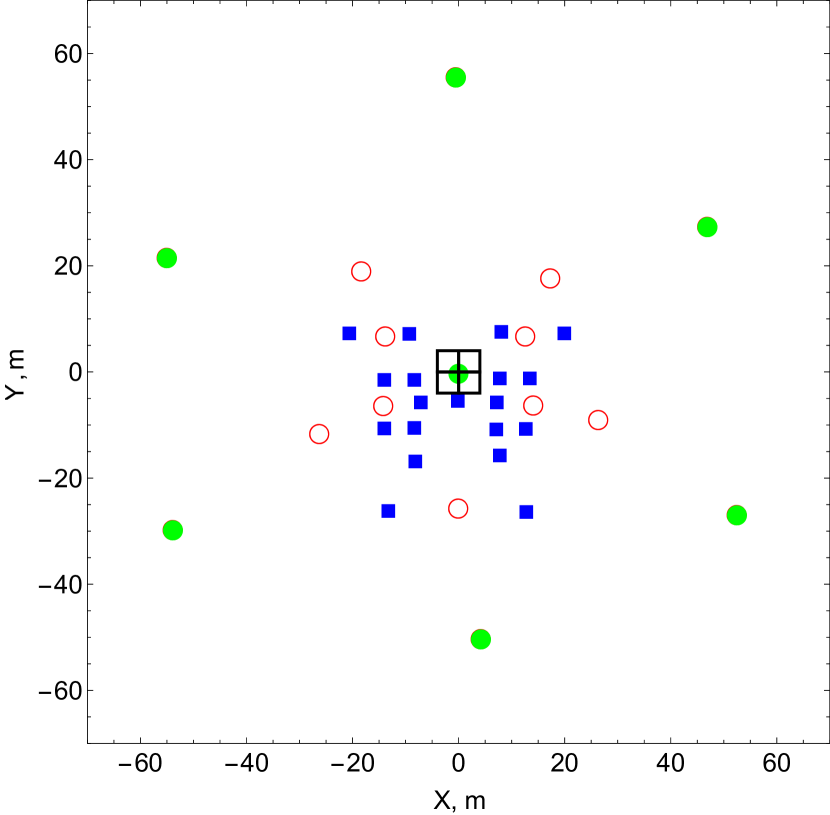
(a)

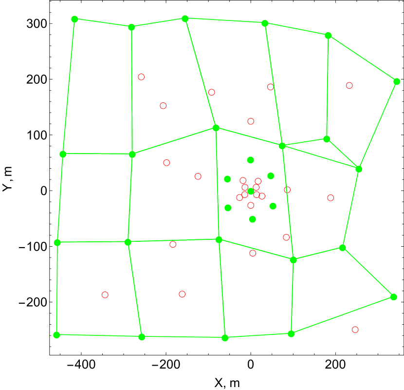
(b)

Figure 1: The EAS-MSU array setup: (a) the central part of the array; (b) the entire array. Four empty black squares in the center represent the special central room. Green circles denote “vans” with scintillation counters, empty red circles denote “vans” without scintillation counters, blue squares denote “boxes”. Lines represent the tetragons of the peripheral trigger system. See the text for more details.

3 The event reconstruction procedure and selection cuts

Reconstruction.

The procedure for the determination of the parameters of a EAS consists of several stages. First, EAS arrival angles (the zenith angle, $\theta$, and the azimuth angle, $\phi$) are calculated analytically from the response times of three scintillation detectors colocated with the counters which recorded the highest density of charged particles [11]. Further, the found angles are used as the first approximation for the arrival direction. The readings of 10 to 15, depending on the size of the shower, charged-particle stations with the highest density, together with the angles, allow to determine the EAS axis position $(X,Y)$ in the plane of the array, the total number of particles $N_{e}$ and the EAS age parameter $S$ in the first approximation. To this end, the method of least squares is used for the lateral distribution function described below. Then, by making use of time delays of all triggered scintillation counters and of the axis position, the EAS arrival direction is recalculated by the method of the maximum likelihood function [11]. Further, using these new $\theta$ and $\phi$, the EAS position, $N_{e}$ and $S$ are recalculated. These iterations continue until the process converges.

The key ingredient of the reconstruction procedure is the lateral distribution function (LDF). It was obtained experimentally [12] by the analysis of showers with $\theta<30^{\circ}$. These showers were divided into 19 groups according to the total number of particles, starting with $\log_{10}N_{e}=4.6$ and with 0.2 dex step, and, for each group, the mean LDF of charged particles was constructed. Then, the empirical LDF was determined by the following procedure. The Nishimura–Kamata–Greisen (NKG) [13, 14] function was taken as the first approximation. Then, keeping in mind that the NKG function is relevant for electrons and positrons while the installation detects other particles as well, the concept of the local age parameter, $S_{\rm local}$, was introduced. The correction to the NKG function was parametrized by the dependence of this $S_{\rm local}$ on the distance $\color[rgb]{0,0,0}r\color[rgb]{0,0,0}$ to the shower axis, so that the effective $S_{\rm local}(\color[rgb]{0,0,0}r\color[rgb]{0,0,0})$ replaces the shower age in the NKG formula. The mean experimental LDF is flatter than the original NKG function both at distances $\color[rgb]{0,0,0}r\color[rgb]{0,0,0}>30$ m and $\color[rgb]{0,0,0}r\color[rgb]{0,0,0}<15$ m. Therefore, the charged-particle LDF we use is

$$\rho(S,\color[rgb]{0,0,0}r\color[rgb]{0,0,0})=N_{e}C(S)(\color[rgb]{0,0,0}r\color[rgb]{0,0,0}/R_{0})^{(S+\alpha(\color[rgb]{0,0,0}r\color[rgb]{0,0,0})-2)}\cdot(\color[rgb]{0,0,0}r\color[rgb]{0,0,0}/R_{0}+1)^{(S+\alpha(\color[rgb]{0,0,0}r\color[rgb]{0,0,0})-4.5)},$$ (3.1)

where $\rho$ is the particle density, $R_{0}\approx 80$ m is the Moliere radius, $S$ is the age parameter of the EAS, which corresponds to the NKG age determined at 15 m$\,\color[rgb]{0,0,0}\lesssim r\lesssim\color[rgb]{0,0,0}\,$30 m, $C(S)$ is the normalization coefficient, which is calculated numerically, and $\alpha(\color[rgb]{0,0,0}r\color[rgb]{0,0,0})$ is the correction to $S$ determined empirically and shown in Fig. 2.

Figure 2: The correction $\alpha(\color[rgb]{0,0,0}r\color[rgb]{0,0,0})$ to the age parameter as a function of the distance from the shower axis $\color[rgb]{0,0,0}r\color[rgb]{0,0,0}$.

Event selection.

In order to study well-reconstructed showers with primary energies exceeding $E\sim 10^{17}$ eV, we apply the following selection cuts:

1. The reconstruction procedure converges and allows to determine the shower parameters.

2. The age parameter of the EAS is $0.3<S<1.8$.

3. The zenith angle is $\theta<30^{\circ}$.

4. The distance between the array center and the shower axis is $R<240$ m.

5. The shower size is $N_{e}>2\times 10^{7}$ (showers with these $N_{e}$ are recorded by the peripheral selection system mostly).

4 Monte-Carlo simulations

The full Monte-Carlo (MC) simulation of the EAS-MSU data includes the following steps, described in more detail below:

(i) simulation of a library of air showers with random arrival directions;

(ii) generation of random locations of the shower axis;

(iii) simulation of the response of the detector stations and recording the simulated event in the format used for real data;

(iv) reconstruction of the event parameters with the standard procedure described in Sec. 3.

Air-shower simulations.

For the first step, we use the CORSIKA 7.4001 [9] simulation package. For the standard simulated event set, we choose the QGSJET-II-04 [15] as the high-energy hadronic interaction model and FLUKA2011.2c [16] as the low-energy hadronic interaction model. The EGS4 [17] electromagnetic model is used for electromagnetic processes. As this combination of modern interaction models gives a good description of the installation, we did not study the effect of change in the models.

At this step, a shower library is produced containing, presently, 1370 artificial showers (852 induced by primary protons and 518 induced by primary iron nuclei). Each shower in the library may be used multiple times at the step (ii). The primary energies of the showers in the library follow the $E^{-1}$ differential spectrum with $10^{\color[rgb]{0,0,0}7.5}$ GeV$<E<10^{\color[rgb]{0,0,0}8.75}$ GeV. These EAS are simulated with zenith angles in the range between $0^{0}$ and $\color[rgb]{0,0,0}35^{0}\color[rgb]{0,0,0}$ assuming an isotropic distribution of arrival directions in the celestial sphere. The showers are simulated without thinning. The lower energy thresholds are fixed for hadrons (excluding $\pi^{0}$) and muons as 50 MeV; for photons, $e^{+}$, $e^{-}$ and $\pi^{0}$ as 250 keV. The standard geomagnetic field for the array location is assumed, $B_{x}=16.5~{}\mu$T and $B_{z}=49.6~{}\mu$T. For definiteness, we fix the model of the atmosphere corresponding to Central Europe for October 14, 1993 (the model number 7 in CORSIKA notations).

Simulation of the detector.

To further process the CORSIKA showers, we use a model of the EAS-MSU facility implemented as a C$++$ code. The showers from the library are randomly selected in such a way that the resulting differential spectrum $dN/dE\sim E^{-3.1}$ is obtained. This spectrum was taken as an approximate fit of combined data presented in Ref. [18], not taking into account the “second knee” feature. For each of the selected showers, we generate a random position of the center on the ground in the array area (more precisely, in the rectangle $|X|<280$ m, $|Y|<280$ m, containing all registrations points plus $50$ m in each direction). We consider three model primary compositions: pure proton, pure iron and a two-component p/Fe mixture with a ratio of components fixed from the data/MC comparison, see below. We also tested the original spectrum measured by EAS-MSU [3] and approximated as $dN/dE\sim E^{-3.04}$, as well as the proton/iron mixtures describing the results of other experiments, namely KASCADE–Grande [19] (59% iron, 41% proton) and Tunka-133 [20] (51% iron, 49% proton for Tunka-133). The impact of these variations on the behavior of the observables ($R$, $\theta$, $N_{e}$) was found negligible.

Given the coordinates and momenta of all particles at the ground level provided by CORSIKA, we test geometrically which of these particles hit a detector station within the facility. For the registration points laying at various heights, we assume that every particle moves with a given velocity and without any interactions forth/back in the direction it has at the ground level. We neglect the interactions of particles with materials covering registration points (typically it is a few millimetres of metal plus a few centimetres of wood), implying it is a part of the atmosphere. We also simulate muon detectors located in a deep underground chamber. For vertically falling particles the shielding of this array amounts to 40 m of water equivalent. Simulating these detectors we select only muons ($\mu^{+}$ and $\mu^{-}$; the electromagnetic contamination is far below one per cent level) whose continuous-slowing-down approximation (CSDA) range in water exceeds its path into shielding material. In turn the CSDA range for muon in water is given by

$$(l_{\rm stop}/\mbox{cm})\simeq 229.69+412.14\,(E_{\mu}/\mbox{GeV})-0.71819\,(E_{\mu}/\mbox{GeV})^{2},$$

where $E_{\mu}$ is the muon energy and $l_{\rm stop}$ is the distance at which the particle loses all its kinetic energy. The approximation is a fit to the data of Ref. [21]. For vertical muons the threshold energy yields approximately 10 GeV. The data/MC comparison for the muon counters will be studied elsewhere.

In our model, the Geiger–Mueller detector response is simulated as follows. During the onset of the shower, each counter can be activated only once, due to its long dead time ($40~{}\mu$s). Thus the measured value is the number of activated counters in a detector. The outer registration points, “vans”, can measure charged-particle density $\rho_{e}$ in limits from $\rho_{e}\approx 0.42$ m^-2 to $\rho_{e}\approx 1750$ m^-2. The same limits for the inner registration points, “boxes”, are from $\rho_{e}\approx 0.64$ m^-2 to $\rho_{e}\approx 117$ m^-2. The counter itself is a tube of glass with $1$ mm thick wall and $0.1$ mm germanium spraying from inside. We assume that a counter is activated for every charged particle hitting the tube. For photons with energy $E_{\gamma}\gtrsim 1$ keV, we use a formula for the interaction probability

$$P_{\rm int}=0.011-0.058/\ln(E_{\gamma}/\mbox{keV})+(E_{\gamma}/\mbox{keV})^{-0.695}.$$

We obtain it as a numerical approximation of the data from Ref. [18], from where we take the total cross section of photon-induced processes in silicon and germanium with charged particles in the final state. A subtlety is that both the cross section and the interaction probability grow with decrease of the photon energy, making the resulting signal sensitive to low-energy photons. In order to estimate the impact of the soft photons on the $N_{e}$ reconstruction, we have performed simulations with the 50 keV cutoff for gamma rays (which is the lowest value allowed by CORSIKA). We obtained that the contribution of photons to Geiger-Mueller counters activation is about 10% of that of charged particles, while in the case of 250 keV gamma-ray cutoff it is about 7%.

In the EAS-MSU experiment, each scintillator measured only the time of its activation. Thresholds for scintillator activation, averaged over the zenith angle, are $1/3$ and $1$ minimal ionizing particles, for peripheral scintillators and the central scintillator, respectively. We use the response functions presented in Ref. [22]. For photons, we make an approximation, randomly choosing only $1/5$ of them and amplifying the response by the factor of 5. This is justified because of the smooth, monotonic character of the response function.

The luminescence time of scintillators is $\sim 1~{}\mu$s (the signal was integrated over $5~{}\mu$s), this leads to the accumulation of particles during the full time of the shower development. For each of the central-system scintillators, we calculate the time of its activation relative to the time of the central scintillator activation with 5 ns resolution. For a peripheral system scintillator, we calculate the time of its activation relative to the time of the first activated peripheral scintillator. According to the EAS-MSU native data format, the result is recorded as a rough part, with 100 ns resolution, and a precise part, with 3.8 ns resolution.

After processing all particles in the shower, the resulting detector signals are written to a file of the same structure as the experimental data files. This file has the size of 1024 kb per event. Each box is encoded in 1 byte which contains a number of activated counters in this box. The timing of each central system scintillator is encoded in 1 byte, while the timing of a peripheral-system scintillator is encoded in 2 bytes, one for the rough part and another for the precise part. Other bytes in the data file either are empty or contain technical information (date, time, type of trigger activated etc.)

The simulation of the experiment does not incorporate the daily calibration information, which includes the following details. In the real facility, some detectors were inactive from one day to another. In our simulation, we neglect this fact because the fraction of these detectors is not large (about a few percent) at any day. For further data processing, e.g. to estimate primary fluxes, this should be included in the exposure, so that the effective area of the array is used as a function of date. We also neglect changes made in cable optical lengths for the central scintillator system and in time resolution of the precise part of the peripheral scintillator system timing. Both of these variations are of order of a few percent and affect the timing record. We approximate these values by its averages.

5 Comparison of data with the simulation

An important part of the EAS-MSU array Monte-Carlo simulation is the comparison of data and MC. This allows to verify the precision of the simulated event set in its representation of the real data set and to demonstrate the reliability of event-selection procedures. Here, we present results of this comparison for reconstructed $N_{e}>2\times 10^{7}$. After applying all quality cuts, the real data sample contains 922 events, while the MC sample contains 4468 proton-induced and 1093 iron-induced showers. They were generated from 852 and 518 independent CORSIKA showers, respectively. When stated explicitly, the data/MC comparison is performed separately for proton and iron primaries. However, as we will discuss in detail below, the data allow for determination of the best-fit primary composition experimentally, from the distribution of the age parameter $S$, assuming the two-component proton-iron mixture. This best-fit composition (43% protons and 57% iron, see item 3 below for its determination) is used for most of the tests throughout the paper.

It is instructive to trace the effect of various cuts on the number of events. This is done in Table 1.

Table 1: Number of independent and resampled CORSIKA showers and the effect of various cuts on the number of events in Monte-Carlo and in real data. Note that we are interested in $N_{e}>2\times 10^{7}$ and simulated showers with $E>10^{16.5}$ eV only, while the installation recorded also events with much lower energies, which explains a large amount of data events not passed the $N_{e}$ cut. The geometric area where the artificial showers are thrown 1.3 times exceeds the area where they are selected.

	MC, p	MC, Fe	data
CORSIKA EAS	852	518	–
sampled EAS	63060	21481	–
triggered EAS	58927	21073	892321
reconstructed EAS,$0.3<S<1.8$	58814	21052	843086
$R<240$ m	37987	13574	702238
$\theta<30^{\circ}$	29283	10249	546493
$N_{e}>2\times 10^{7}$	4468	1093	922
all cuts	4468	1093	922

1. Geometry and the primary arrival direction.

The key observables of an air shower are the arrival direction and the core position; all other recorded parameters are very sensitive to the geometry. Figures 3 and

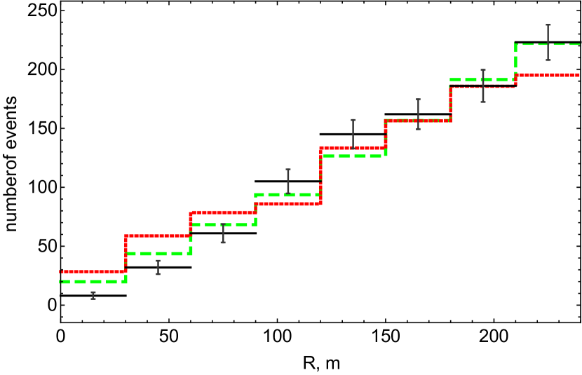
(a)

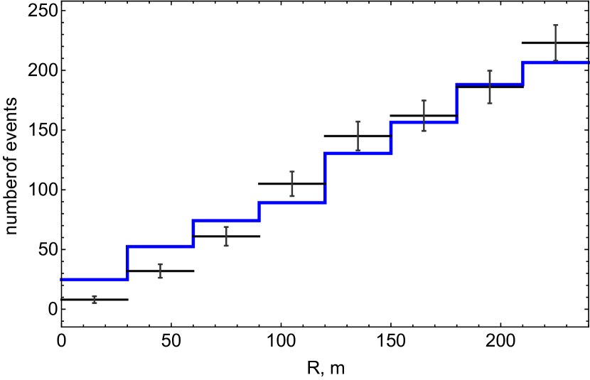
(b)

Figure 3: Data versus MC comparison of the distribution in $R$. Points with error bars: data. (a): green dashed hystogram: MC (protons), red dotted hystogram: MC (iron); (b): blue hystogram: MC (the best-fit composition).

4

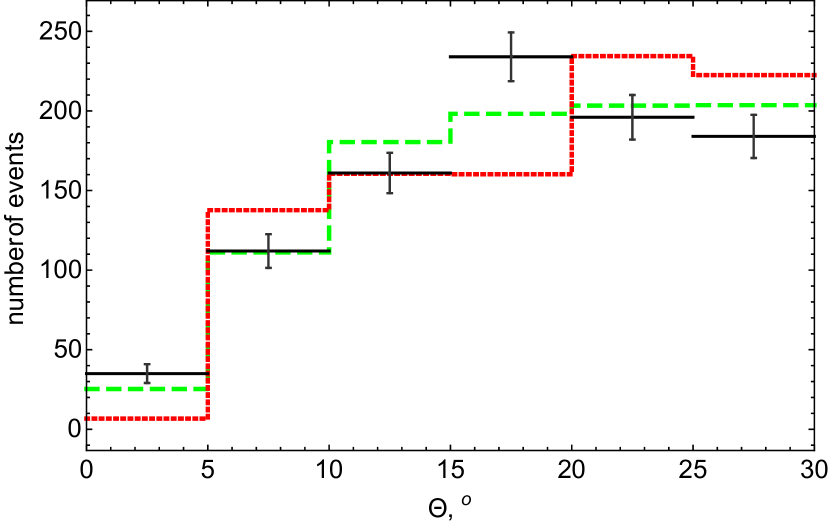
(a)

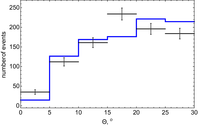
(b)

Figure 4: Data versus MC comparison of the distribution in $\theta$. Points with error bars: data. (a): green dashed hystogram: MC (protons), red dotted hystogram: MC (iron); (b): blue hystogram: MC (the best-fit composition).

present comparisons between the distributions of the real and MC events in the distance between the axis and the array center $R$ and the zenith angle $\theta$, respectively (all histograms in the paper are normalized to the number of events in the real data sample after all cuts, that is 922) . Comparison between the known trajectory of the thrown MC primary particle and its reconstructed parameters allows one to determine the accuracy with which the position of the shower axis and the arrival direction are determined, see Figs. 5 and 6, respectively.

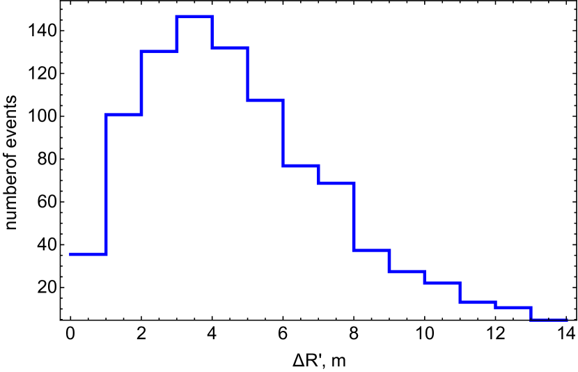
Figure 5: Distribution of distances between thrown and reconstructed MC position of the point where the shower axis crosses the array plane, in meters (the best-fit composition).

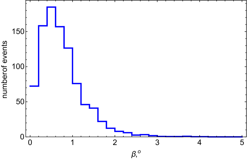
Figure 6: Distribution of the angular separation between thrown and reconstructed MC arrival direction, in degrees (the best-fit composition).

The estimated reconstruction accuracy is presented in Table 2.

Table 2: Accuracy of the reconstruction for $N_{e}>2\times 10^{7}$ determined from the Monte-Carlo simulations (the best-fit composition). 68% of the events are reconstructed with the precision not worse than the quoted values.

axis position, m	5.7
arrival direction, degree	1.1
$\Delta N_{e}/N_{e}$	0.165
$\Delta E/E$	0.41

2. Shower size and the primary energy.

The distribution in the reconstructed $N_{e}$ agrees well between the real and simulated data sets, see Fig. 7.

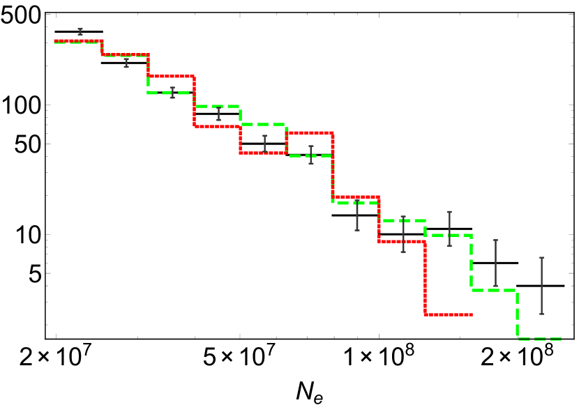
(a)

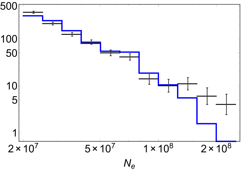
(b)

Figure 7: Data and MC comparison of the distribution in $N_{e}$. Points with error bars: data. (a): green dashed hystogram: MC (protons), red dotted hystogram: MC (iron); (b): blue hystogram: MC (the best-fit composition).

This supports the use of the chosen thrown spectrum as a first approximation.

Figure 8

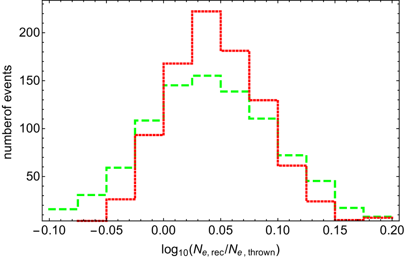
(a)

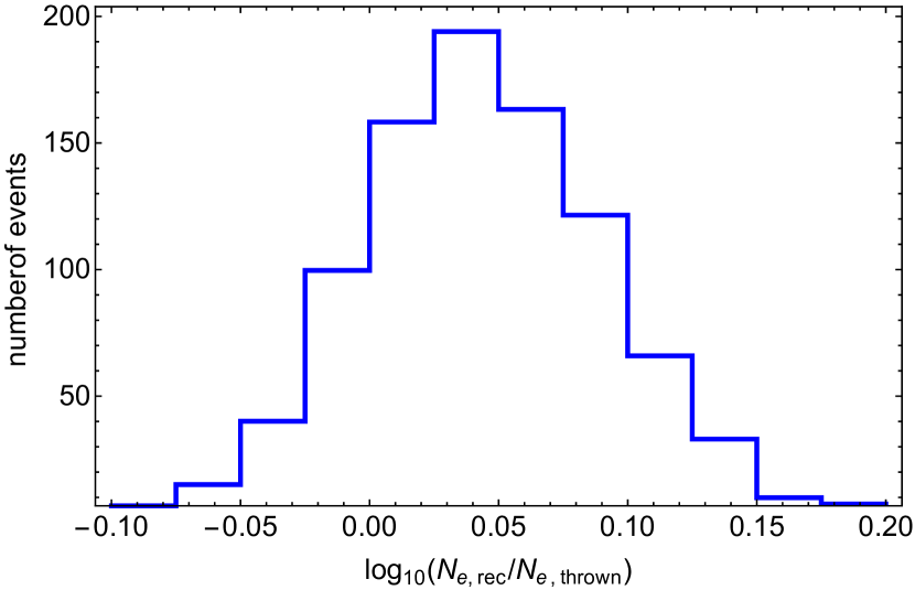
(b)

Figure 8: Distribution of ratios of the reconstructed $N_{e}$ to the “thrown” $N_{e}$ which is the total number of charged particles from the CORSIKA output supplemented by the contribution of photons to the signal, see the text, for MC events. (a): green dashed hystogram: MC (protons), red dotted hystogram: MC (iron); (b): blue hystogram: MC (the best-fit composition).

illustrates the accuracy of the reconstruction of $N_{e}$ in comparison with the total number of charged particles and interacting photons in counter calculated by CORSIKA. The relative bias of $\sim 7\%$ may be attributed to the difference in the definitions of the number of charged particles in a shower. The accuracy of the $N_{e}$ determination is also presented in Table 2. Note that it decreases with energy reaching $\sim 0.15$ for the highest energies we consider.

The relation between $N_{e}$ and the primary energy is model-dependent in simulations and always depends on the type of the primary particle. From our simulations, we may estimate it for the QGSJET-II-04 model we use. Figure 9

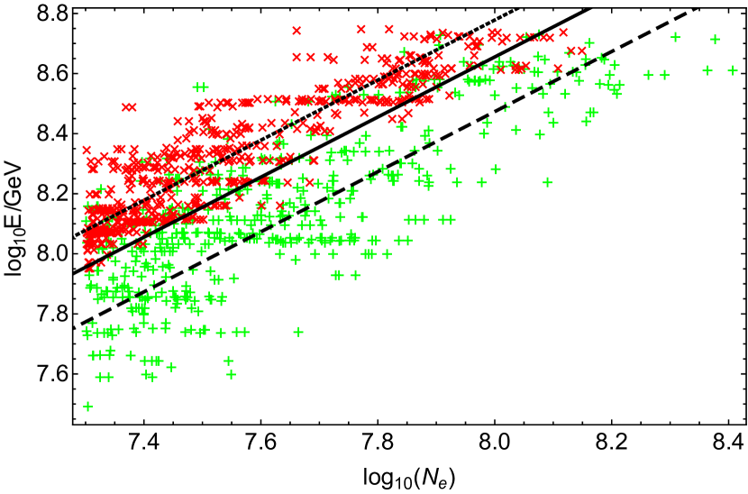
Figure 9: Thrown energy $E$ versus reconstructed $N_{e}$ for the MC events: green pluses – primary protons, red crosses – primary iron. The full line represents the relation (5.1), the dashed and dotted lines represent the relations for primary protons and iron, respectively.

presents, for the proton and iron primaries, the scatter plot of thrown energies and reconstructed values of $N_{e}$. The following relations may be obtained, through a fit,for primary protons,

$$\log_{10}\left(\frac{E_{\rm p}}{\rm GeV}\right)=(0.47\pm 0.01)+\log_{10}N_{e},$$

and for primary iron nuclei,

$$\log_{10}\left(\frac{E_{\rm Fe}}{\rm GeV}\right)=(0.78\pm 0.01)+\log_{10}N_{e},$$

respectively. Here, we assumed that $E\propto N_{e}$. This is justified for a short energy range we consider (one decade); allowing for a power-law dependence, $E\propto N_{e}^{a}$, gives $a$ very close to unity, but with a less stable fit. For practical reasons, however, we need a “$N_{e}$–$E$” relation which may be used without the knowledge of the primary type, as is relevant for the real data. We make use of our working best-fit composition to obtain an average relation,

$$\log_{10}\left(\frac{E}{\rm GeV}\right)=0.65+\log_{10}N_{e}.$$ (5.1)

Note that, contrary to similar relations for scintillator detector arrays, Eq. (5.1) does not include the zenith angle $\theta$. This approximation is feasible because the shower age is taken into account in the LDF and only $\theta\leq 30^{\circ}$ showers are analyzed.

Having Eq. (5.1) as a working model for the energy estimation of hadronic primaries, one may estimate the accuracy of the energy reconstruction by comparison of the thrown MC energy and the energy calculated from the reconstructed $N_{e}$ by means of Eq. (5.1). This comparison is illustrated in Fig. 10

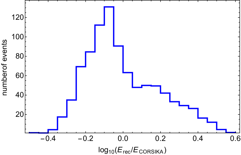
Figure 10: Distribution of ratios of the energy $E$, calculated by means of Eq. (5.1) from the reconstructed $N_{e}$, to the thrown primary energy, for the MC events (the best-fit composition).

and the resulting accuracy is quoted in Table 2.

Shower age and the primary composition.

The reconstruction of geometrical parameters discussed above is insensitive to the type of the primary particle of an EAS. However, the shower age parameter $S$, which is related to the depth of the shower development in the atmosphere and is reconstructed in the LDF fit, is composition-sensitive. As a result, the distributions of the MC events in $S$ differ significantly for the proton and iron primaries, see Fig. 11 (a).

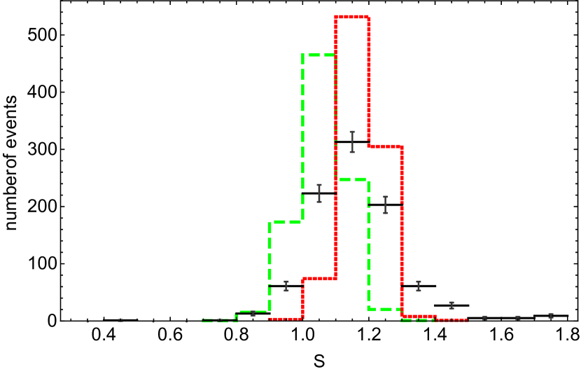
(a)

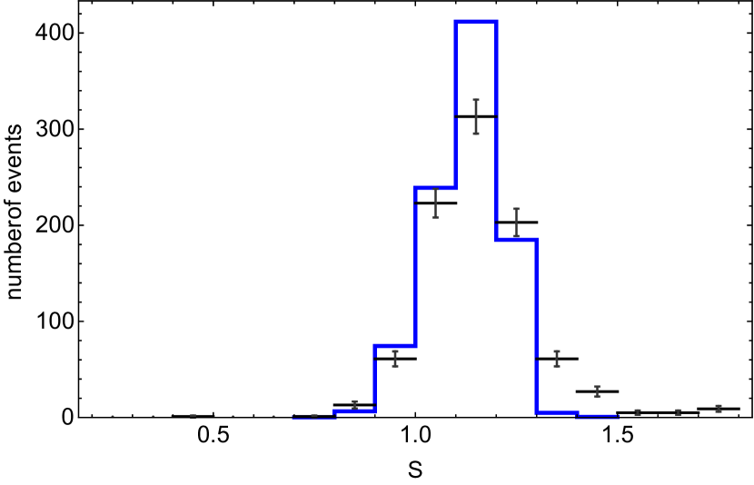
(b)

Figure 11: Data and MC comparison of the distribution in $S$. Points with error bars: data. (a) Green dashed hystogram: MC (protons); red dotted hystogram: MC (iron). (b) Blue hystogram: MC (the best-fit composition).

Therefore, we have used the data distribution over $S$ to derive the relevant primary composition. The best-fit composition appears to be almost energy-independent in the energy range we consider, $\sim(10^{17}-10^{18})$ eV (though the highest-energy part of the data set is statistically depleted). For the two-component model we use, it includes $\approx 43\%$ of protons and $\approx 57\%$ of iron. The comparison between data and MC mixed according to this composition is presented in Figs. 11 (b), 12.

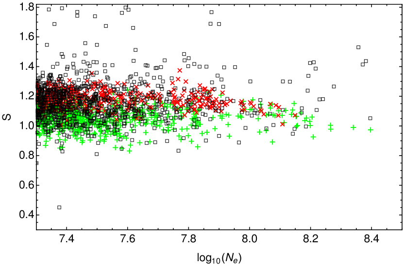
Figure 12: The shower age parameter $S$ vs $N_{e}$. Boxes: data; green pluses: MC (protons); red crosses: MC (iron).

It is the composition we used for basic data/MC comparison tests throughout the paper. A good agreement of data and MC in $S$ obtained for the realistic primary composition represents a non-trivial test of our full MC model of the EAS-MSU installation. The result obtained for the chemical composition from the fit of the $S$ distribution with a proton/iron mixture may be considered as approximate; it is the composition assumed for the considered model of the detector only. Nevertheless our result shows good agreement with more robust results of other experiments e.g. KASCADE-Grande [19] and Tunka-133 [20].

Discussion.

The overall data/MC agreement is good, which justifies the use of our MC model of the detector for future studies. However, a detailed examination of the plots reveals minor disagreements in distributions of some reconstructed observables, mainly in tails. In particular, there is a minor excess of events with large $S$ in data with respect to simulations. These events, about a few per cent of the data set, are probably caused by some detector saturation effect related to occasional unrecorded technical problems in the particle-detection system. Saturation effects can be caused by the technique of the measurement of the charged-particle density, $\rho_{c}$. As it was mentioned in Sec. 2, each detector station in the peripheral system contains 72 large counters, 24 medium counters and 24 small counters. The charged particle density is estimated as $\rho_{c}=\ln\left(n/(n-m)\right)/A$, where $n$ is the number of counters in the detector station, $m$ is the number of fired counters and $A$ is the area of the counter. This yields the following limits of $\rho_{c}$ measurement: from $0.42$ m^-2 to $130$ m^-2 for large counters, from $4.3$ m^-2 to $318$ m^-2 for medium counters and from $23.6$ m^-2 to $1766$ m^-2 for small counters. As a default, for every detector station, $\rho_{c}$ is calculated from readings of the large counters. However, once all the large counters are fired, $\rho_{c}$ is calculated from readings of medium counters. The same rule applies to medium and small counters. There could exist, however, situation when all large or medium counters are hit by shower particles, while some of the counters didn’t trigger due to the hardware failure. This could lead to a significant underestimation of $\rho_{c}$ at this detector station. This effect can only reduce the particle density recorded by a given detector close to the shower axis, leading to a flatter LDF (i.e. to higher $S$ and $N_{e}$ parameters) and to a light overestimation of $R$. The latter happens due to high concentration of detector stations in the center of array. Actually, the possibility of one or two undetection errors in each detector station is taken into account in the reconstruction program but other errors of the same nature still could lead to the same effect, which we call the saturation effect. While the usual saturation is accounted for in all our simulations, we are unable to trace these possible undocumented errors and to model them. We suppose that these unresolved errors are responsible for the minor discrepancy between MC and data for small $R$ in Fig. 3, for large $N_{e}$ in Fig. 7 (and, consequently, for large $E$ in Fig. 10) and for large $S$ in Figs. 11, 12. Note that these events imitate old showers and cannot mimic gamma-ray induced events, which develop deeper in the atmosphere, see e.g. Refs. [23, 24], while the study of primary gamma rays, to be reported in a separate publication, is the main motivation for the present work.

6 Conclusions

To summarize, we presented a full chain of Monte-Carlo simulations of air showers developing in the atmosphere, being detected by the EAS-MSU array and reconstructed by the procedure equivalent to that used for the real data. We have verified that the simulation describes well the distribution of the data in basic parameters. Assuming a modern hadronic-interaction model, we obtained a relation between the reconstructed shower size $N_{e}$ and the primary energy $E$. We used our Monte-Carlo event sets to estimate the accuracy of the reconstruction of the shower geometry, $N_{e}$ and energy. Forthcoming studies will use these simulations to reanalyze data on $E_{\mu}>10$ GeV muons in the air showers recorded by the installation, which will open the possibility to test, within modern frameworks, the origin of the apparent excess of muonless events seen in the EAS-MSU data.

References

- [1] S. N. Vernov et al., New Installation Of Moscow State University For Studying Extensive Air Showers With Energies To eV, Bull. Russ. Acad. Sci. Phys. 44 (1980) 80 [Izv. Ross. Akad. Nauk Ser. Fiz. 44 (1980) 537].
- [2] G. V. Kulikov, G. B. Khristiansen, On the Size Spectrum of Extensive Air Showers, Sov. Phys. JETP 8 (1959) 441 [Zh. Exp. Teor. Fiz. 35 (1958) 635].
- [3] Yu.A. Fomin et al., Energy spectrum of cosmic rays at energies eV, Proc. 22nd Int. Cosmic Ray Conf., Dublin 2 (1991) 85.
- [4] G. B. Khristiansen et al., Primary cosmic ray mass composition at energies eV to eV as measured by the MSU EAS array, Astropart. Phys. 2 (1994) 127.
- [5] Yu. A. Fomin et al., Nuclear composition of primary cosmic rays in the ’knee’ region according MSU EAS array data, J. Phys. G 22 (1996) 1839.
- [6] N. Kalmykov, J. Cotzomi, V. Sulakov and Yu. A. Fomin, Primary cosmic ray composition at energies from to eV according to the EAS MSU array data, Bull. Russ. Acad. Sci. Phys. 73 (2009) 547 [Izv. Ross. Akad. Nauk Ser. Fiz. 73 (2009) 584].
- [7] Yu. A. Fomin et al., Estimate of the fraction of primary photons in the cosmic-ray flux at energies eV from the EAS-MSU experiment data, J. Exp. Theor. Phys. 117 (2013) 1011 [Zh. Exp. Teor. Fiz. 144 (2013) 1153]. [arXiv:1307.4988 [astro-ph.HE]].
- [8] Y. A. Fomin et al., Estimates of the cosmic gamma-ray flux at PeV to EeV energies from the EAS-MSU experiment data, JETP Lett. 100 (2015) 699 [arXiv:1410.2599 [astro-ph.HE]].
- [9] D. Heck et al., CORSIKA: A Monte Carlo code to simulate extensive air showers, Tech. Rep. 6019, FZKA (1998)
- [10] T. Abu-Zayyad et al. [Telescope Array Collaboration], CORSIKA Simulation of the Telescope Array Surface Detector, arXiv:1403.0644 [astro-ph.IM].
- [11] G.B. Khristiansen, G.V. Kulikov, Yu.A. Fomin. Cosmic Rays of Superhigh Energies, Karl Tiemig Verlag, Munchen, 1980, 246 p.
- [12] N.N. Kalmykov, G.V. Kulikov, V.P. Sulakov, Yu.A. Fomin, On the choice of the lateral distribution function for EAS charged particles, Bull. Rus. Acad. Sci.: Physics 71 (2007) 522 [Izv. Ross. Acad. Nauk Ser. Fiz. 71 (2007) 539].
- [13] K. Kamata, J. Nishimura, The Lateral and the Angular Structure Functions of Electron Showers, Prog. Theor. Phys. Suppl. 6 (1958) 93.
- [14] K. Greisen, Cosmic ray showers, Ann. Rev. Nucl. Part. Sci. 10 (1960) 63.
- [15] S. Ostapchenko, Monte Carlo treatment of hadronic interactions in enhanced Pomeron scheme: I. QGSJET-II model, Phys. Rev. D 83 (2011) 014018 [arXiv:1010.1869 [hep-ph]].
- [16] G. Battistoni et al., The FLUKA code: Description and benchmarking, AIP Conf. Proc. 896 (2007) 31.
- [17] W. R. Nelson, H. Hirayama, D. W. O. Rogers, The EGS4 code system, Tech. Rep. 0265, SLAC (1985).
- [18] K. A. Olive et al. [Particle Data Group Collaboration], Review of Particle Physics, Chin. Phys. C 38 (2014) 090001.
- [19] J. C. Arteaga-Velazquez et al., The KASCADE-Grande observatory and the composition of very high-energy cosmic rays, J. Phys. Conf. Ser. 651 (2015) 012001.
- [20] S. F. Berezhnev et al., Tunka-133: Primary Cosmic Ray Energy Spectrum in the energy range eV, Proc. 32nd ICRC, Beijing 1 (2011) 209.
- [21] D. E. Groom, N. V. Mokhov and S. I. Striganov, Muon stopping power and range tables 10 MeV to 100 TeV, Atom. Data Nucl. Data Tabl. 78 (2001) 183.
- [22] N. Sakaki et al., Energy estimation of AGASA events, Proceedings of ICRC 2001, 329 (2001).
- [23] M. Risse and P. Homola, Search for ultrahigh energy photons using air showers, Mod. Phys. Lett. A 22 (2007) 749 [astro-ph/0702632 [ASTRO-PH]].
- [24] O. E. Kalashev, G. I. Rubtsov and S. V. Troitsky, Sensitivity of cosmic-ray experiments to ultra-high-energy photons: reconstruction of the spectrum and limits on the superheavy dark matter, Phys. Rev. D 80 (2009) 103006 [arXiv:0812.1020 [astro-ph]].