CLEX: Yet Another Supercomputer Architecture?

Abstract

We propose the CLEX supercomputer topology and routing scheme. We prove that CLEX can utilize a constant fraction of the total bandwidth for point-to-point communication, at delays proportional to the sum of the number of intermediate hops and the maximum physical distance between any two nodes. Moreover, all-to-all communication can be realized $(1+o(1))$-optimally both with regard to bandwidth and delays. This is achieved at node degrees of $n^{\varepsilon}$, for an arbitrary small constant $\varepsilon\in(0,1]$. In contrast, these results are impossible in any network featuring constant or polylogarithmic node degrees. Through simulation, we assess the benefits of an implementation of the proposed communication strategy. Our results indicate that, for a million processors, CLEX can increase bandwidth utilization and reduce average routing path length by at least factors $10$ respectively $5$ in comparison to a torus network. Furthermore, the CLEX communication scheme features several other properties, such as deadlock-freedom, inherent fault-tolerance, and canonical partition into smaller subsystems.

I Introduction & Related Work

Ever since the advent of massively parallel computing architectures, there has been lively interest in the question how the nodes of a supercomputer should be interconnected, e.g. as a fat tree, butterfly, or hypercube [1, 2, 3, 4, 5, 6, 7, 8, 9, 10, 11, 12, 13]. Naturally, these topologies try to balance between the desires for small node degrees and short routing paths. Moreover, it is crucial to serve routing requests in parallel, using little, distributed computation, and to deal with faults. Eventually, the theoretical understanding of these issues became systematic and mature [14, 15, 16, 17].

Today, communication in supercomputers is by and large implemented by means of low-degree interconnection topologies. Thus, one would expect to find the well-analysed topologies that have been proposed decades ago to dominate the market. But far from it! State-of-the-art architectures like Cray XMT or IBM Blue Gene provide point-to-point communication on top of a three-dimensional torus network [18, 19]. This appealing simplicity in design comes at a cost, as such a system is fundamentally limited in communication. Konecny [19] writes “Because the most interesting mode of operation assumes uniformly distributed traffic, the network performance is expected to be dominated by the bisection bandwidth.” In a three-dimensional torus of $n=k^{3}$ processors, one can partition the processors such that two subsets of $n/2$ processors are connected by $2k^{2}$ edges only. In other words, because of communication limitations “the third dimension” of processing is lost, since the average point-to-point bandwidth between these subsets scales with $2/k$ times the individual link capacity. Bluntly, in today’s supercomputers, for $n\approx 10^{6}$ processors the torus architecture restricts communication to less than 1% of the total available bandwidth in the worst case.

So why is it that such an apparently suboptimal design is chosen by practitioners? We believe the answer to this question to be twofold. On the one hand, a (locally) grid-like communication network is of course well-suited to deal with communication patterns that are local as well. We argue, however, that this approach has several shortcomings. Firstly, it restricts the range of problems for which the computer architecture is fitting to problems that are parallelizable in a way that matches the network topology. Secondly, programmers need to be aware of this issue and program accordingly, which might be a non-trivial and error-prone task. Thirdly, on large scales, load balancing issues may result in more complex, less local communication patterns if an efficient progress of computation is to be ensured. And finally, even if all these issues can be overcome at the time when the system goes online, it will typically be in use for several years, implying that it is difficult to predict whether demands will change during the life-time of the supercomputer.

On the other hand, the theory on interconnection networks fails to address some questions of practical significance. For one, how should one actually realize one of the suggested topologies? This turns out to be critical for performance, as the efficiency of the whole communication infrastructure might break down because some of the physical links are exceedingly long: these connections will suffer larger communication delays, consume more space and energy, and complicate the physical layout of the system. To the best of our knowledge, this issue has been neglected in all theoretical studies of the matter; in stark contrast, even for the three-dimensional torus, which is fairly amenable to low-distortion “embedding”, optimizing the stretch has been considered a worthwhile task [20]. What is more, we believe it to be important to devise routing algorithms that deal with faults in a seamless, fully distributed, and automatic manner. Therefore, it is not enough to show that a topology exhibits a large number of disjoint short path between to destinations, but one also needs to give a routing scheme that exploits the high connectivity of the system to establish robustness with respect to failing nodes or links.

In consequence, we would like to revive the interconnection discussion from a theoretical point of view by presenting a new topology we call CLEX (CLique-EXpander). Essentially, the CLEX design is the result of seeking efficient communication in a world of physical constraints. To this end, we deviate from standard analysis by measuring delays not solely in terms of hops, but also considering the physical distance a signal needs to travel. We prove that a point-to-point communication bandwidth per node (to and from arbitrary destinations) matching the total bandwidth per node up to a constant factor can be achieved, at delays that are (asymptotically) proportional to the maximum physical distance between any two nodes. Moreover, applying an asymmetric bandwidth assignment to the links, all-to-all communication can be realized $(1+o(1))$-optimally both with regard to bandwidth and delays.

As constant or polylogarithmic node degrees necessarily incur an average hop distance of $\Omega(\log n/\log\log n)$, the price we pay for these properties are node degrees of $n^{\varepsilon}$, for an arbitrarily small constant $\varepsilon$. However, these fairly high degrees are “localized” in the sense that all but a constant number of them connect the nodes of the basic building blocks of our topology, i.e., cliques of size $n^{\varepsilon}$. Thus, one way to interpret our results is to view the CLEX approach as a method to localize the issue of an efficient (low-degree) communication network to much smaller systems of $n^{\varepsilon}$ nodes, which may e.g. reside on a single multi-core board. A multi-core board will offer means of on-board communication by itself, and due to small distances and integrated circuits one can expect it to be of greater efficiency than that of a comparable large-scale network. Thus, the high connectivity of a CLEX system could be considered an abstraction that can be replaced by any efficient local communication scheme within the cliques (cf. e.g. [7]).

Nonetheless, we do also propose a routing scheme that indeed is designed for the high-degree CLEX network as is. Within cliques, it employs recent results on parallel randomized load balancing [23], ensuring a high degree of efficiency and resilience of the overall approach. From our point of view, the properties of the resulting system justify to re-raise the question whether high degrees can be worth the effort. In fact, one could see this as another step of localization: Our algorithm reduces the routing problem on the clique level to one on the node level, namely to the one of efficiently routing between $n^{\varepsilon}$ input and output ports. This task now is to be solved on a physically much smaller scale, dealing with smaller communication delays and being able to rely on much better synchronization between the individual components. Again, one is free to replace the full connectivity between the ports by any combination of topology and routing scheme that is efficient at this scale.

To add some salt to the above theoretical considerations, we assess the efficiency of a CLEX architecture in practice. To this end, we simulate point-to-point communication in two systems comprising $32^{4}\approx 1,000,000$ nodes and $64^{3}\approx 250,000$ nodes. The results of our simulation indicate that the usable bandwidth of a CLEX architecture could be an order of magnitude larger than the theoretical optimum of the IBM Blue Gene and Cray XMT tori interconnection networks. Since our comparison assumes identical total bandwidth in both designs, this is not a mere consequence of indirectly increasing bandwidth via node degrees, but a fundamental difference of the underlying topologies.

II Topology and Routing Algorithms

In this section, we give solutions to the all-to-all and point-to-point communication problems. To this end, we define an abstract model amenable to formal analysis. However, the applied proof techniques extend to stronger models which better match a real-world system. In particular, the assumptions of asynchronicity and fault-free behaviour can be dropped. After describing the topology of the CLEX architecture, we briefly compare two algorithms solving all-to-all communication efficiently on our topology and the three-dimensional torus. Finally, we give an algorithm for point-to-point communication and analyze its synchronous running time. Our theoretical findings are supported by the simulations presented in Section III.

II-A Model and Problem Formulation

We model a supercomputer as an undirected graph $G=(V,E)$, $n:=|V|$, where nodes represent the computing elements (processors) and edges bidirectional communication links. To simplify the presentation, we assume that for each $v\in V$, the loop $\{v,v\}$ is contained in $E$, i.e., nodes may “send messages to themselves”. We assume that communication is reliable and proceeds in synchronous rounds. Message size is in $\Omega(\log n)$, i.e., we assume that a constant number of node identifiers of size $\log n$ fits into a message. Any upper bound on the message size respecting this constraint is feasible; for the purpose of our analysis, we however assume that in each round only one “unit payload” can be sent by each node along each edge. Nodes have access to an infinite source of random bits. We point out, however, that our algorithms will in practice work reliably also with pseudo-random instead of true random bits, since all our results hold with high probability (w.h.p.)

Note that the assumptions on the communication model (which simplify the presentation) can be considerably relaxed. Our algorithms can be run asynchronously by including round counters into messages. Furthermore, as demonstrated in [23], the load balancing scheme can be made resilient to a constant (independent) probability of message loss.

Observe that the total delay a message suffers comprises the time it takes being relayed at intermediate nodes plus the time the signal travels along the edges of the interconnection network. Thus, the simplistic measure given by round complexity may not be accurate in practice; we also need to understand the influence of propagation times. Therefore, we define the maximal (average) delay $d$ ($\bar{d}$) as

$$d:=c_{h}h+c_{p}p\quad\mbox{and}\quad\bar{d}:=c_{h}\bar{h}+c_{p}\bar{p},$$

where $h$ ($\bar{h}$) is the maximal (average) number of hops until a message is delivered, $p$ ($\bar{p}$) is the maximal (average) physical distance a message travels, and $c_{h}$ and $c_{p}$ are appropriate constants (comprising units). To get an idea of the order of magnitude of the respective terms, suppose that it takes a few clock cycles before a message can be relayed (to a free channel) and clock speeds are in the order of gigahertz. Thus, forwarding a message is initiated after a few nanoseconds. At speed of light, a signal travels about a foot per nanosecond.

Formally, we will solve the following problems.

Problem II.1 (Point-to-Point Communication)

Each node $v$ is given a (finite) set of messages

$${\cal S}_{v}=\{m_{v}^{i}\,|\,i\in\{1,\ldots,i_{v}^{\max}\}\}$$

with destinations $d(m_{v}^{i})\in V$. The goal is to deliver all messages to their destinations, minimizing delays. By

$${\cal R}_{v}:=\big{\{}m_{w}^{i}\in\cup_{w\in V}{\cal S}_{w}\,\big{|}\,d(m_{w}^{i})=v\big{\}}$$

we denote the set of messages a node $v\in V$ shall receive. We abbreviate $\mathbf{S}:=\max_{v\in V}|{\cal S}_{v}|$ and $\mathbf{R}:=\max_{v\in V}|{\cal R}_{v}|$, i.e., the maximal numbers of messages a single node needs to send or receive, respectively.

All-to-all communication is a special case of point-to-point communication.

Problem II.2 (All-To-All Communication)

Each node $v\in V$ is given a message $m_{v}$. The goal is to deliver (a copy of) each message $m_{v}$ to all nodes, minimizing delay.

Note that this problem is easier to solve, since by setting ${\cal S}_{v}=\{m_{v}^{w}\,|\,w\in V\}$ and $d(m_{v}^{w})=w$ an instance of Problem II.1 is obtained.

II-B Interconnection Network

Evidently, with node degrees of at most $\Delta$, any algorithm for Problem II.2 must take at least $n/\Delta$ rounds to complete. Similarly, Problem II.1 cannot be solved in less than $\max\{\lceil{\mathbf{S}}/\Delta\rceil,\lceil{\mathbf{R}}/\Delta\rceil\}$ rounds, as no node can send or receive more than $\Delta$ messages in each round. Thus, in order to hope for good running times, the communication graph needs to expand very quickly, i.e., for any set of nodes $S\subset V$ with $|S|\leq n/2$ it is necessary that $S$ has $\Omega(\Delta|S|)$ outgoing edges. At the same time, we need to be aware that long-range links bridging a large physical distance should not be used frequently, which needs to be respected by our routing scheme and thus also the underlying topology. This motivates the following recursive graph construction.

Definition II.3 (CLEX Graphs)

Suppose for a constant $s\in(0,1]$ that $n^{s}$ and $1/s$ are integer. We recursively define the (directed) CLEX graph $\mathrm{C}(s,l)$ of $l\in\{1,\ldots,1/s\}$ levels. Set $\mathrm{C}(s,1):=K_{n^{s}}$, i.e., a clique of $n^{s}$ nodes, and label its nodes $(1),(2),\ldots,(n^{s})$. Assuming that $\mathrm{C}(s,l)$ is already defined, $\mathrm{C}(s,l+1)$ is composed of $n^{s}$ isomorphic copies $\mathrm{C}(s,l)_{i}$, $i\in\{1,\ldots,n^{s}\}$, plus additional edges. Using the label $(v_{1},\ldots,v_{l})\in\{1,\ldots,n^{s}\}^{l}$ a node $v\in V(\mathrm{C}(s,l))_{i}$ inherits from $\mathrm{C}(s,l)_{i}$, we can identify it uniquely with $(v_{1},\ldots,v_{l},i)\in\{1,\ldots,n^{s}\}^{l+1}$.

The edges of $\mathrm{C}(s,l+1)$ are all edges contained in the $\mathrm{C}(s,l)_{i}$ plus

$$E_{i,l+1} := \{((v_{1},\ldots,v_{l},i),(v_{1},\ldots,v_{l-1},j,v_{l}))$$

$$~{}|\,j\in\{1,\ldots,n^{s}\}\wedge v\in V(\mathrm{C}(s,l)_{i})\},$$

i.e., $E(\mathrm{C}(s,l+1))=\cup_{i=1}^{n^{s}}(E(\mathrm{C}(s,l)_{i})\cup E_{i,l+1})$. See Figures 2 and 2 for an illustration.

(a)

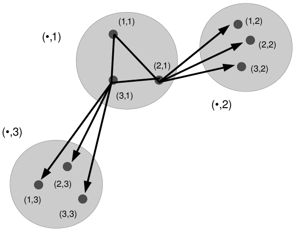
Figure 1: Illustration of $C(1/3,2)$. Each copy of $C(1/3,1)$ is enclosed in a grey circle. The links without arrowheads are bidirectional. For clarity, only the outgoing links of the nodes in the center copy are depicted, and the redundant links of node $(1,1)$ on level $1$ (connecting to the nodes of the first copy) are left out.

(a)

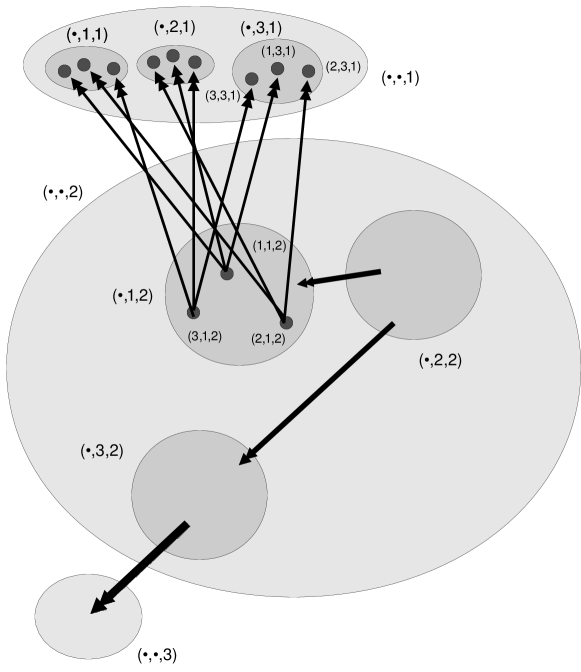
Figure 2: Illustration of the level $2$ links of $C(1/3,3)$. Copies of $C(1/3,2)$ and $C(1/3,1)$ are enclosed by light and dark grey circles, respectively. Only the outgoing links of nodes in the center copy of $C(1/3,1)$ are depicted. The remaining arrows subsume the connections of the copies of $C(1/3,1)$ labeled $(\cdot,2,2)$ and $(\cdot,3,2)$. Note that it is not necessary to connect the subgraphs on level 2 or higher precisely in this way, as long as bandwidths are well-balanced on each level.

Observe that each copy of $\mathrm{C}(s,l+1)$ connects each of its subgraphs $\mathrm{C}(s,l)_{i}$ by $|V(\mathrm{C}(s,l))|$ many edges to any $\mathrm{C}(s,l)_{j}$, $j\in 1,\ldots,n^{s}$, such that degrees increase by exactly $n^{s}$ on each level. Thus, $\mathrm{C}(s,1/s)$ has uniform degrees of $n^{s}/s-1$. Its diameter $D(\mathrm{C}(s,1/s))$ is bounded by $2^{s}-1$, as $D(K_{n_{s}})=1$ and $D(\mathrm{C}(s,l+1))$ is at most $2D(\mathrm{C}(s,l))+1$. We remark that these graphs are not Cayley graphs (cf. [14]).

Note that if for any $k,t\in\mathbb{N}$ we set $n:=k^{t}$ and $s:=1/t$, both $1/s$ and $n^{s}$ are integer, i.e., $\mathrm{C}(s,l)$ is defined for $l\in\{1,\ldots,t\}$. In other words, it is possible to choose $s$ arbitrarily small and $n$ arbitrarily large.

The CLEX topology can be realized with e.g. a grid-like node positioning. We ensure that nodes that are connected on low levels are close to each other by arranging them in cubes. On each new level, we simply arrange an appropriate number of cubes to a larger cube. Such a system will not experience a significant stretch in distances due to embedding issues.

As will emerge from the analysis, it is feasible to replace nodes’ $n^{s}$ edges in $E_{i,l+1}$ by a single link of capacity $n^{s}$ to one of the endpoints of these edges (such that each node gets also exactly one incoming link of this capacity). This is also compatible with the solution of Problem II.2 proposed in Section II-C. Note that this way, node degrees become $n^{s}+1/s-2$, with merely $1/s-1$ long-range links (i.e., links that are not on the basic level). Clearly, this is to be preferred in any real-world system, however, for ease of presentation, we stick to uniform edge capacities in our exposition.

II-C All-to-All Communication

Problem II.2 has simple solutions both on the torus and on CLEX graphs. On the torus, first nodes exchange all messages in $x$-direction, then $y$-, and finally $z$-direction. This defines for each message a tree with the source as root on which the message is flooded. Thus this scheme is bandwidth-optimal up to factor three. If links are congested, i.e., the necessary traffic exceeds the available bandwidth, asymptotic optimality with regard to delays follows from this observation. On the other hand, in absence of congestion the solution is also delay-optimal, as the trees have minimal depth. For the CLEX design, things are less obvious.

We will show that physical average and maximal routing path lengths can also be kept close to the optimum in CLEX systems. For the sake of simplicity, throughout this paper we assume that the torus is (locally) a perfect three-dimensional grid of $k_{1}\cdot k_{2}\cdot k_{3}$ nodes. We assume that the CLEX topology is realized in a hierarchical cube structure as described in Section II-B. We assume that cable connections are as short as possible, for both considered topologies.

Using the previously explained scheme to solve Problem II.2 on the torus, messages travel on average $\bar{h}^{T}=(k_{1}+k_{2}+k_{3})/2\geq 3n^{1/3}/2$ many hops. Hence, the maximal delay in an uncongested setting would be roughly proportional to this value. Observe that no architecture can perform significantly better, as processors cannot be packed much more densely because of cooling issues and physical routing path lengths are optimal up to a factor of $\sqrt{3}$.

The strategy to solve Problem II.2 on $\mathrm{C}(s,1/s)$ is very similar to the one for tori. Each message $m_{v}$ is flooded along a tree induced by with respect to hop distance shortest paths from $v$ to all nodes, where links on lower levels are preferred (because they bridge shorter distances), giving a bandwidth-optimal solution up to factor $1/s$, since links on level one have to deal with most of the load. Note that an asymmetric bandwidth assignment to the different levels reduces this factor, cf. Section III-A. Messages are delivered to all destinations after travelling at most one edge on each level. Since we assumed that processors are arranged in a cubic grid and links are direct connections, maximal link lengths on Level $l\in\{1,\ldots,1/s\}$ are $\sqrt{3}n^{ls/3}/2$, i.e., maximal propagation delays are

$$c_{p}\bar{p}=c_{p}\frac{\sqrt{3}n^{1/3}}{2}\sum_{i=0}^{1/s-1}n^{-is/3}\in c_{p}\frac{(1+o(1))\sqrt{3}n^{1/3}}{2}.$$

Hence, we achieve a $(1+o(1))$-approximation to physically optimal delays in $C(s,1/s)$, which on three-dimensional tori is impossible. For the test settings presented in Section III, the $(1+o(1))$ term is close to $\sqrt{3}$, i.e., the algorithm will at least perform as good as any solution on a torus interconnection network with regard to propagation delays.

Moreover, as observed in Section II-B, the diameter of $\mathrm{C}(s,1/s)$ is $2^{1/s}-1$, i.e., messages make at most that many hops. For fixed $s$, we thus achieve asymptotically optimal maximal delays $d$ proportional to the maximal spatial distance between any two nodes. For the parameter values considered in Section III, the number of hops reduces about a factor $10$ in comparison to a torus network of the same size. As in a torus network typically the number of hops will be the dominant factor contributing to delays in all-to-all communication, a CLEX network promises a considerable improvement.

II-D Point-to-Point Communication

In the following, w.l.o.g. we assume that in Problem II.1 $\mathbf{S}=\mathbf{R}$, as e.g. in case $\mathbf{S}<\mathbf{R}$ the number of messages each node needs to send is upper bounded by $\mathbf{R}$ (and we want to show a bound that is essentially linear in $\mathbf{S}+\mathbf{R}$). Rerouting each message through a uniformly and independently at random (u.i.r.) chosen intermediate node (i.e., applying Valiant’s trick [24]), we need to solve the two slightly simpler problems that $(i)$ each node needs to send at most $\mathbf{S}$ messages whose destinations are distributed u.i.r. or $(ii)$ each node needs to receive at most $\mathbf{R}$ messages whose origins are distributed u.i.r. Note that these problems are (asymptotically speaking) indeed less difficult, as applying Chernoff’s bound we see that w.h.p., in the first case each node needs to receive at most $\mathbf{R}^{\prime}\in(1+o(1))\mathbf{S}$ messages, while in the second case, no node initially holds more than $\mathbf{S}^{\prime}=\mathbf{R}^{\prime}$ many messages. Thus, for the sake of analyzing the asymptotic complexity of the problem, w.l.o.g. we assume in the following that message destinations are distributed u.i.r.

We proceed by defining and analyzing the Algorithms $\mathcal{A}(l)$, $l\in\{1,\ldots,1/s\}$, which solve Problem II.1 on $\mathrm{C}(s,l)$. In case of $l=1$, the communication graph is simply $K_{n^{s}}$, thus we can use an algorithm suitable for complete graphs. The advantage of full connectivity is that any node may serve as relay for any message, reducing the routing problem to a load balancing task. We follow the approach from [23]. For the sake of clarity, we present a simplified algorithm to illustrate the concept. Initialize $i:=1$ and $k(1):=1$ at each node. The algorithm executes the following loop until all messages are delivered:

1. Create $\lfloor k(i)\rfloor$ copies of each message. Distribute these copies uniformly at random among all nodes, but under the constraint that (up to one) all nodes receive the same number of messages.

2. To each node, forward one copy of a message destined to it (if any has been received in the previous step; any choice is feasible). Confirm this to the original sender of the message.

3. Delete all messages for which confirmations have been received and all currently held copies of messages.

4. Set $k(i+1):=\min\{k(i)e^{\lfloor k(i)\rfloor/5},\sqrt{\log n}\}$ and $i:=i+1$.

Intuitively, this algorithm exploits that the number of messages that still needs to be delivered falls rapidly, thus enabling the nodes to try routing increasingly many redundant copies of the remaining messages without causing too much traffic. If just one of these copies can be deleted, the message will not participate in the subsequent phase. Hence the number of messages will fall by a factor that is exponential in the number of copies per message, permitting to use an exponentially larger number of copies in the next phase without overloading the communication network.

The techniques and proofs presented in [23] yield the following bound on the running time of this simple algorithm for the special case of $\mathbf{S}=\mathbf{R}=n$.

Corollary II.4

Provided that $\mathbf{S}=\mathbf{R}=n$, the above algorithm solves Problem II.1 in $\mathcal{O}(\log^{*}n)$ synchronous rounds w.h.p., where $\log^{*}x$ denotes the inverse tower function. ∎

For ease of presentation, we do not discuss asynchronicity (which is dealt with by round counters) or the case that $\mathbf{S},\mathbf{R}\neq n$ (requiring to adapt the growth of $k$) here. In [23] appropriate modifications of the given algorithm are discussed, leading to the following more general result.

Corollary II.5

An algorithm $\mathcal{A}(1)$ exists that solves Problem II.1 in an asynchronous system within $\mathcal{O}((\mathbf{S}+\mathbf{R})/n+(\log^{*}n-\log^{*}(n/\mathbf{R})))$ time w.h.p.

It is important to note that $\mathcal{A}(1)$ is not uniform, i.e., (an appropriate estimate of) $\mathbf{S}+\mathbf{R}$ needs to be known to the nodes in order to execute the algorithm. However, it is not difficult to guarantee this in a practical system by monitoring the network load and updating the nodes frequently. Also, instead of the “one-shot” version of the problem described, a perpetually running solution is required that handles the network traffic generated over time. We argue, however, that in light of the results from [23], it is feasible to study the simplified version of the problem in order to assess the potential gain of our approach.

Having $\mathcal{A}(1)$ in place, we rely on recursion to solve the task on Level $l>1$:

1. Calling $\mathcal{A}(l-1)$, node $v\in\mathrm{C}(s,l-1)_{i}$, $i\in\{1,\ldots,n^{s}\}$, sends each of its messages to a node in $\mathrm{C}(s,l-1)_{i}$ whose edges in $E_{i,l}$ lead to the copy of $\mathrm{C}(s,l-1)$ containing the destination of the message, choosing u.i.r. from the nodes fulfilling this criterion.

2. Each node forwards the received messages over its edges in $E_{i,l}$ to the copy of $\mathrm{C}(s,l-1)$ they are destined for, balancing the load on these edges.

3. $\mathcal{A}(l-1)$ is called again to forward all messages to their destinations.

We will show now that this algorithm is asymptotically optimal with respect to the number of hops (i.e., required rounds) up to a small term inherited from $\mathcal{A}(1)$.

Theorem II.6

Algorithm $\mathcal{A}(1/s)$ solves Problem II.1 on $\mathrm{C}(s,1/s)$. Its running time is w.h.p. bounded by $\mathcal{O}((\mathbf{S}+\mathbf{R})/n^{s}+(\log^{*}n^{s}-\log^{*}(n^{s}/\mathbf{R}))$.

Proof:

We prove the statement by induction on $l\in\{1,\ldots,1/s\}$, i.e., we show that for any $l$, $\mathcal{A}(l)$ solves Problem II.1 on $\mathrm{C}(s,l)$ within the stated number of rounds w.h.p. For $l=1$ this claim immediatelz follows from Corollary II.5. Observe that for $l>1$, $\mathcal{A}(l)$ will eventually deliver all messages to their destinations since $\mathcal{A}(1)$ does, i.e., it is sufficient to show the stated bound on the running time. Moreover, note that it does not matter how the constants in the $\mathcal{O}$-term grow with $l$ since $l$ is constantly bounded.

Assume that the claim is correct for some $l\in\{1,\ldots,1/s-1\}$. We show that whenever $\mathcal{A}(l+1)$ calls $\mathcal{A}(l)$, w.h.p. at most $\mathcal{O}(\mathbf{S}+\mathbf{R}+\log n)$ many messages have to be sent or received by any node. Recalling that message destinations are w.l.o.g. distributed u.i.r., we have that the at most $\mathbf{R}|V(\mathrm{C}(s,l)|$ messages that have destinations in some given copy of $V(\mathrm{C}(s,l)$ are distributed u.i.r. among all copies of $V(\mathrm{C}(s,l)$. Hence, between any pair $V(\mathrm{C}(s,l)_{i}$, $V(\mathrm{C}(s,l)_{j}$ of such copies, in expectation at most $\mathbf{R}|V(\mathrm{C}(s,l))|/n^{s}$ messages need to be exchanged. Thus, Chernoff’s bound yields that w.h.p. no more than $\mathcal{O}(\mathbf{R}|V(\mathrm{C}(s,l))|/n^{s}+\log n)$ messages need to be sent from $V(\mathrm{C}(s,l)_{i}$ to $V(\mathrm{C}(s,l)_{j}$.

Afterwards, applying Chernoff’s bound again, we infer that the number of messages a single node needs to receive in Step 1 is w.h.p. at most $\mathcal{O}(\mathbf{R}+\log n)$, as a fraction of $1/n^{s}$ of the nodes in $V(\mathrm{C}(s,l)_{i}$ have edges in $E_{i,l}$ that lead to $V(\mathrm{C}(s,l)_{j}$. By induction hypothesis, each call of $\mathcal{A}(l)$ in Step 1 will thus terminate within $\mathcal{O}((\mathbf{S}+\mathbf{R})/n^{s}+(\log^{*}n^{s}-\log^{*}(n^{s}/\mathbf{R})))$. rounds w.h.p. Moreover, as for each node its $n^{s}$ edges in $E_{i,l}$ lead to the same copy of $\mathrm{C}(s,l)$, Step 2 terminates in $\mathcal{O}((\mathbf{R}+\log n)/n^{s})=\mathcal{O}(R/n^{s})$ rounds w.h.p. In addition, this implies that no node will have to send more than $\mathcal{O}(R)$ messages in Step 3 w.h.p. Hence, we can apply the induction hypothesis again in order to see that Step 3 terminates within $\mathcal{O}((\mathbf{S}+\mathbf{R})/n^{s}+(\log^{*}n^{s}-\log^{*}(n^{s}/\mathbf{R})))$ rounds w.h.p. This concludes the induction step and the proof.

A closer examination of the involved constants reveals that they grow exponentially in $1/s$. However, in recursive calls the algorithm uses exclusively links on lower levels. Since the number of nodes on each level grows rapidly, the physical distances of the nodes grow by more than factor 2 for each added level. Thus, overall routing path length is bounded by a geometric series with constant limit times the lengths of links on the top level. On the other hand, since we will choose $s$ not too small ($1/3$ resp. $1/4$), the number of routing hops is still small.

We remark that it is possible to generalize Theorem II.6 to non-constant values of $1/s\in\mathcal{O}(\sqrt{\log n/\log\log n})$, however, choosing $s$ too small is not desirable since the number of routing hops grows exponentially in $1/s$.

III Performance Estimation

In this section, we study the practical merits that are to be expected from implementing the proposed communication strategy. We base our reasoning on simulation results and discuss in detail what effects on bandwidth and delays of arbitrary point-to-point communication can be deduced in comparison to a torus network. Furthermore, we briefly address some advantages regarding the robustness of the proposed routing scheme.

III-A Dense Traffic (Bandwidth Comparison)

Theorem II.6 states an asymptotic result, i.e., for sufficiently large $n$ and any constant $s\in(0,1)$, outdegrees of $n^{s}+1/s-2$ suffice to guarantee good load balance and a running time that is only a constant factor larger than the optimum. However, it is not clear how large the number of nodes needs to be for a certain value of $s$ in order to ensure good performance. The strong probability bounds obtained in Section II-D indicate that the approach is quite robust, therefore good results for practical values of $n$ can be expected.

In order to estimate the bandwidth and delays a CLEX system will feature in comparison to a torus grid of the same size and total bandwidth, we performed simulations of the proposed point-to-point communication algorithm on $\mathrm{C}(1/4,4)$ with $n=32^{4}\approx 10^{6}$ and on $\mathrm{C}(1/3,3)$ with $n=64^{3}\approx 2.5\cdot 10^{5}$ nodes. Due to memory constraints, we confined ourselves to simulating the algorithm synchronously and solving recursive calls iteratively one after another. As pointed out earlier, both algorithm and analysis are resilient to asynchronicity; hence, neither parallel nor sequentially executed recursive calls interfere with each other, implying that the obtained results should allow for a valid performance estimation of a real-world system.

Furthermore, we adapted the algorithm from Section II-D slightly. Firstly, we are primarily interested in the case of uniformly distributed traffic, i.e., there is no need for the algorithm to establish a uniform distribution of messages by itself. Thus, we do not apply Valiant’s trick here, but rather start with uniformly distributed destinations. Note that in case of “somewhat, but not entirely uniform” distributions, it is easy to apply a “lightweight” version of Valiant’s trick: just redistribute the messages uniformly within e.g. level $1/s-1$ or $1/s-2$ clusters. This drastically reduces the factor 2 overhead incurred by Valiant’s trick, both with respect to the number of hops and the distance messages travel. Secondly, for $l>1$, in Step 2 of $\mathcal{A}(l)$ we choose the subset of neighbors receiving one message more than the others uniformly at random; this slightly improves the load balance. Thirdly, when calling $\mathcal{A}(1)$ on the subgraphs $\mathrm{C}(1,s)$, nodes initially send along each link one message (if available) directly to its destination. Hence, a large fraction of the messages require only one hop to reach their (interim) destinations. Finally, to further save bandwidth, nodes may refrain from sending several copies of the remaining messages to potentially relaying nodes. Rather, they merely request a message to be forwarded to its target by a neighbor, which requires negligible $\log(32)+2=7$ respectively $\log(64)+2=8$ bits (the destination’s identifier in the Level-$1$ clique plus a phase counter for all phases after the first in an asynchronous execution of algorithm $\mathcal{A}(1)$, cf. Figure 3). These bits may also be piggybacked on another message. Then, after receiving a positive acknowledgement, the actual message is sent. Though this will delay the messages that are not delivered immediately by two more rounds, we will later see that the accordant delays do not significantly contribute to the total time until a message is delivered.

In a first simulation experiment, we consider almost saturated channels, i.e., each node initially is source for $28\approx 0.9\cdot 32$ respectively $57\approx 0.9\cdot 64$ messages. Unless the communication system gets overloaded (i.e., more messages arrive than can be delivered quickly), it is reasonable to expect that not all nodes generate the same amount of messages. However, due to the randomized allocation of messages to relaying and target nodes, larger average loads support a balanced load distribution (and thus throughput). Hence, we chose to initially assign to all nodes roughly 90% of the messages that can be transferred on a level in a single round, thus permitting a worst-case estimation of the bandwidth utilization under full load while getting useful results with regard to message delays. Message destinations follow a uniformly random permutation of the set containing each node $28$ resp. $57$ times, i.e., each node has to send and receive the same number of messages. Thus, results afford an easy comparison to the values for all-to-all communication given in Section II-C.

For each Level $l$, we measured four values: the maximal number of rounds (excluding recursive calls) that any instance of $\mathcal{A}(l)$ required, the average number of rounds (excluding recursive calls) messages spent on this level in total, the maximal average load per node any instance of $\mathcal{A}(l)$ had to deal with, and the (average) number of edges messages traversed on Level $l$ during the course of the complete algorithm. The outcomes of the measurements are listed in Tables I and II.

TABLE I: $\mathcal{A}(4)$ on $\mathrm{C}(1/4,4)$ with $32^{4}$ nodes, 28 messages from and to each node

​lvl.​	​max. rds.​	​avg. rds.​	​max. avg. load​	​avg. hops​
1	11	13.69	33.44	10.63
2	2	4.11	30.33	4
3	2	2.05	28.06	2
4	2	1.03	28	1

TABLE II: $\mathcal{A}(3)$ on $\mathrm{C}(1/3,3)$ with $64^{3}$ nodes, 57 messages from and to each node

​lvl.​	​max. rds.​	​avg. rds.​	​max. avg. load​	​avg. hops​
1	9	6.90	62.06	5.34
2	2	2.03	57.30	2
3	2	1.01	57	1

We see that loads are well-balanced on all levels; due to the small number of nodes on Level $1$ some instances of $\mathcal{A}(1)$ invoked on $\mathrm{C}(1/4,4)$ are slightly overloaded. Accordingly, the vast majority of the messages can be forwarded immediately on all but the first level, where a different routing scheme is employed. On the first level, a small but relevant fraction of the messages cannot be forwarded at once, leading to delays that are roughly 75% larger than the minimal possible $8$ respectively $4$ rounds. These messages lead to an increase of about 30% in traffic, since they are relayed by other nodes, requiring one additional hop. The large maximal number of rounds $\mathcal{A}(1)$ takes to complete is in accordance with theory. The algorithm runs $\mathcal{O}(\log^{*}n)$ phases w.h.p., where in our implementation the first phase takes 1 round and each subsequent phase 2 rounds; we incur a delay of 2 more rounds due to the modification that relaying messages is preceded by an acknowledged request (except for the first phase). Consequently, the algorithm should terminate within roughly $1+2\log^{*}32=1+2\log^{*}64=7$ rounds, which is true for most instances; the large number of recursive calls and the fact that on $\mathrm{C}(1/3,3)$ some of the calls have higher average loads than nodes’ degrees explain the differences. Figure 3 depicts the number of remaining messages of all invoked instances of $\mathcal{A}(1)$ plotted against the number of passed phases.

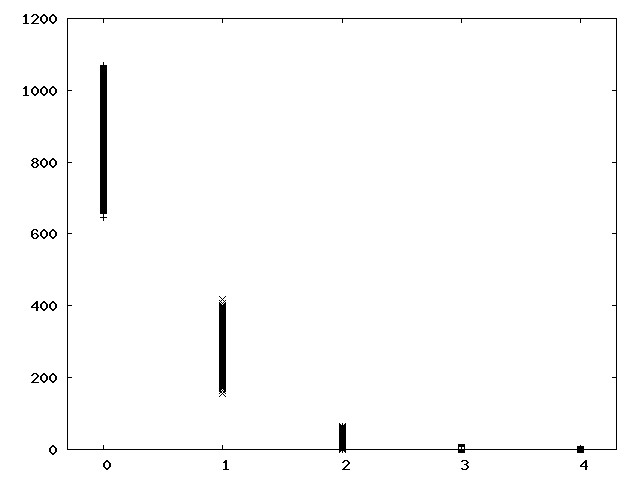
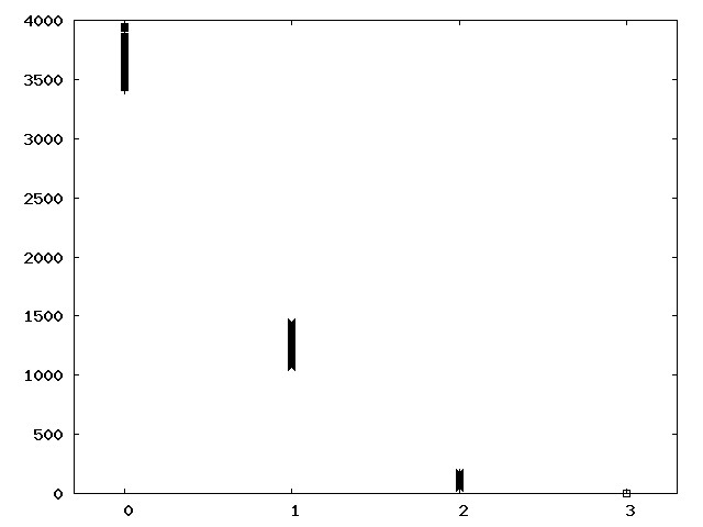
Figure 3: Number of messages instances of $\mathcal{A}(1)$ still needed to deliver against passed phases. Left: $\mathrm{C}(1/4,4)$ with $32^{4}$ nodes and $28$ initial messages per node, right: $\mathrm{C}(1/3,3)$ with $64^{3}$ nodes and $57$ initial messages per node. In both cases most of the instances terminated after three phases; on $\mathrm{C}(1/4,4)$, a single instance required 5 phases.

Note that a single message is unlikely to experience large delays in all calls of $\mathcal{A}(1)$ it participates in. The total number of rounds a message spends on Level $1$ can be stochastically bounded from above by the sum of independent random variables describing the number of rounds passing until a message is forwarded in the most loaded instance of $\mathcal{A}(1)$. Thus, Chernoff type bounds apply, giving exponential tail bounds on the probability that the random variable exceeds its expectation. As on higher levels almost all messages are forwarded immediately, we have a strong indication that few messages will be delayed more than 2-2.5 times the expected average delay, both with respect to hops and propagation time.

Due to the increase of the number of nodes on each level by a factor of 32 (64), the physical distances of the processors—and hence the length of connecting cables—grow by factor $32^{1/3}\approx 3.2$ ($64^{1/3}=4$) per level. On the top level, link lengths will be in the order of the network diameter. Shortest-path routing in a torus grid bridges on average similar distances as one hop on the top level of $\mathrm{C}(s,1/s)$. We conclude a worst-case bound on the competitive ratio with respect to $\bar{p}$ of about (cf. Tables I and II)

$$2.5 \approx 1.03+\frac{2.05}{3.2}+\frac{4.11}{3.2^{2}}+\frac{13.69}{3.2^{3}}$$

$$\mbox{resp.}\quad 2 \approx 1.01+\frac{2.03}{4}+\frac{6.90}{4^{2}}$$

in comparison to the theoretical optimum in a torus grid that does not suffer from congestion. In contrast, the average number of hop delays decreases by factors

$$7.3 \approx \frac{3\cdot 32^{4/3}}{2(1.03+2.05+4.11+13.69)}$$

$$\mbox{resp.}\quad 9.7 \approx \frac{3\cdot 64^{3}}{2(1.01+2.03+6.90)}.$$

Recalling that delays in torus networks are dominated by the time it takes to forward messages, we deduce that CLEX architectures will feature significantly smaller overall message delays even when close to maximal communication load.

Next, we compare the bandwidth we provide to each node to the theoretical optimum in a three-dimensional torus interconnection network. In both settings, the topology appears identical to each node. Therefore, it is reasonable to assume that each node has the same total bandwidth capacity of $B$. Moreover, the amount of inbound and outbound communication is identical, implying that we can confine our considerations to outgoing messages.

For symmetry reasons, in a torus network of $n=k^{3}$ nodes ($k$ nodes in each spatial direction) an optimal scheme assigns each link the same capacity of $B/6$. We partition the nodes into two sets of equal size, such that the corresponding cut is minimum, containing $2k^{2}$ edges. If message destinations are distributed u.i.r., in expectation every second message needs to pass this cut. Hence, with regard to uniformly distributed traffic, the effective average bandwidth with regard to Problem II.1 provided to each node is bounded from above by $2B/(3n^{1/3})$.

On $\mathrm{C}(s,1/s)$, we assert bandwidth according to the simulation results, i.e., each node first divides its bandwidth to the levels according to the weights given by the average hops messages travelled on each level (cf. Tables I and II) and then the bandwidth on each level evenly among the links on that level. Each message will consume one unit of bandwidth per hop. We conclude that the gain in effective point-to-point bandwidth compared to the theoretical maximum for a torus architecture will be at least roughly

$$8.6 \approx \frac{3\cdot 32^{4/3}}{2(1+2+4+10.63)}$$

$$\mbox{resp.}\quad 11.5 \approx \frac{3\cdot 64}{2(1+2+5.34)}.$$

Recall that the proposed asymmetric assignment of bandwidth also improves the efficiency of the simpler mechanism for all-to-all communication presented in Section II-C. Since most communication takes place on level $1$, to which we assigned the majority of the bandwidth, we achieve a bandwidth utilization for Problem II.2 that is at least 2-competitive, regardless of $s$.

III-B Light Traffic (Delay Comparison)

Total message delays will be smaller if traffic is less dense, since most messages can be forwarded immediately. Consequently, for a fair comparison of delays, we consider light traffic matching the maximum throughput of a torus network. From the previous results we infer that initial loads need to be $4>28/8.6$ and $5>57/11.5$, respectively. Moreover, since saving bandwidth is not crucial any longer, we can refrain from requesting message indirection on the lowest level prior to sending complete messages. Apart from these two modifications, the test settings are identical. The results are given in Tables III and IV.

TABLE III: $\mathcal{A}(4)$ on $\mathrm{C}(1/4,4)$ with $32^{4}$ nodes, 4 messages from and to each node

​lvl.​	​max. rds.​	​avg. rds.​	​max. avg. load​	​avg. hops​
1	5	9.02	9.02	10.53
2	1	4	7.32	4
3	1	2	4.02	2
4	1	1	4	1

TABLE IV: $\mathcal{A}(3)$ on $\mathrm{C}(1/3,3)$ with $64^{3}$ nodes, 5 messages from and to each node

​lvl.​	​max. rds.​	​avg. rds.​	​max. avg. load​	​avg. hops​
1	5	4.32	10.36	5.11
2	1	2	5.09	2
3	1	1	5	1

We observe that dropping the mechanism to save bandwidth reduces delays on Level 1 significantly, while due to the smaller loads the average bandwidth consumption per message is roughly the same as before. Repeating the previous calculations for the new data, we see that average propagation delays slightly improve to at worst (cf. Tables III and IV)

$$2.3 \approx 1+\frac{2}{3.2}+\frac{4}{3.2^{2}}+\frac{9.02}{3.2^{3}}$$

$$\mbox{resp.}\quad 1.8 \approx 1+\frac{2}{4}+\frac{4.32}{4^{2}}$$

times the average time a signal requires to follow physically shortest paths. The required number of hops reduces considerably, widening the gap to torus interconnection networks to factors

$$9.5 \approx \frac{3\cdot 32^{4/3}}{2(1+2+4+9.02)}$$

$$\mbox{resp.}\quad 13.1 \approx \frac{3\cdot 64^{3}}{2(1+2+4.32)}.$$

Moreover, we see that all messages can be forwarded immediately on all but the lowest level and $\mathcal{A}(1)$ terminates after at most 5 rounds in all instances.

IV Conclusion

In this work, we proposed the CLEX interconnection and routing scheme for supercomputers. Our results emphasize the advantages of small diameters when aiming for small delays and high bandwidth utilization in face of growing numbers of processors. We simulated configurations of $3$- respectively $4$-level CLEX architectures comprising half a million and a million nodes. The results indicate performance gains of roughly an order of magnitude for point-to-point communication in comparison to three-dimensional torus topologies. This comparison is based on the principal limitations of a torus topology, i.e., it does for instance not respect that a real-world routing mechanism will not be able to concurrently propagate all messages along shortest paths. Certainly, this performance gap will more than compensate for an increased local switching time due to larger node degrees, and it might justify the larger expense for the routing hardware. We believe this to be particularly true in the future, since in the past (parallel) computation power grew much faster than communication capacity, and there is no sign that this trend might stop anytime soon.

References

- [1] G. B. Adams, III, D. P. Agrawal, and H. J. Seigel, “A Survey and Comparision of Fault-Tolerant Multistage Interconnection Networks,” Computer, vol. 20, no. 6, pp. 14–27, 1987.
- [2] J. H. Ahn, N. Binkert, A. Davis, M. McLaren, and R. S. Schreiber, “Hyperx: topology, routing, and packaging of efficient large-scale networks,” in Proc. Conference on High Performance Computing Networking, Storage and Analysis (SC). New York, NY, USA: ACM, 2009, pp. 1–11.
- [3] J. Goodman and C. Sequin, “Hypertree: A Multiprocessor Interconnection Topology,” IEEE Transactions on Computers, vol. C-30, no. 12, pp. 923–933, Dec. 1981.
- [4] R. I. Greenberg and C. E. Leiserson, “Randomized Routing on Fat-Trees,” in Advances in Computing Research, vol. 5, 1989, pp. 345–374.
- [5] C. Guo, H. Wu, K. Tan, L. Shi, Y. Zhang, and S. Lu, “Dcell: a Scalable and Fault-Tolerant Network Structure for Data Centers,” in SIGCOMM ’08: Proceedings of the ACM SIGCOMM 2008 conference on Data communication. New York, NY, USA: ACM, 2008, pp. 75–86.
- [6] S. Johnsson and C.-T. Ho, “Optimum Broadcasting and Personalized Communication in Hypercubes,” IEEE Transactions on Computers, vol. 38, no. 9, pp. 1249–1268, 1989.
- [7] J. Kim, W. J. Dally, and D. Abts, “Flattened Butterfly: a Cost-Efficient Topology for High-Radix Networks,” in ISCA, 2007, pp. 126–137.
- [8] F. T. Leighton, Introduction to Parallel Algorithms and Architectures: Arrays, Trees, and Hypercubes. San Mateo, CA, USA: Morgan Kaufmann, 1992.
- [9] C. E. Leiserson, Z. S. Abuhamdeh, D. C. Douglas, C. R. Feynman, M. N. Ganmukhi, J. V. Hill, W. D. Hillis, B. C. Kuszmaul, M. A. S. Pierre, D. S. Wells, M. C. Wong-Chan, S.-W. Yang, and R. Zak, “The Network Architecture of the Connection Machine CM-5,” J. Parallel Distrib. Comput., vol. 33, no. 2, pp. 145–158, 1996.
- [10] J. Leonard, “The Kautz Digraph as a Cluster Interconnect,” in Proc. International Conference on High Performance Computing, Networking and Communication Systems (HPCNCS), 2007, pp. 53–58.
- [11] M. T. Raghunath and A. Ranade, “Designing Interconnection Networks for Multi-Level Packaging,” in Proc. of the 1993 ACM/IEEE conference on Supercomputing (Supercomputing ’93), 1993, pp. 772–781.
- [12] H. J. Siegel, W. G. Nation, C. P. Kruskal, and L. M. J. Napolitano, “Using the Multistage Cube Network Topology in Parallel Supercomputers,” Proc. of the IEEE, vol. 77, no. 12, pp. 1932–1953, 1989.
- [13] Y. Zhu, M. Taylor, S. Baden, and C.-K. Cheng, “Advancing Supercomputer Performance through Interconnection Topology Synthesis,” in Proc. IEEE/ACM International Conference on Computer-Aided Design (ICCAD 2008), Nov. 2008, pp. 555–558.
- [14] M.-C. Heydemann, Graph Symmetry: Algebraic Methods and Applications. Kluwer Academic Publishers, 1997, ch. Cayley Graphs and Interconnection Networks, pp. 167–223.
- [15] E. Shamir and A. Schuster, “Communication aspects of networks based on geometric incidence relations,” Theor. Comput. Sci., vol. 64, pp. 83–96, 1989.
- [16] E. Upfal, “An O(log N) deterministic packet-routing scheme,” Journal of the ACM, vol. 39, pp. 55–70, 1992.
- [17] S. Even and A. Litman, “Layered cross product – technique to construct interconnection networks,” Networks, vol. 29, no. 4, pp. 219–223, 1997.
- [18] N. R. Adiga, M. A. Blumrich, D. Chen, P. Coteus, A. Gara, M. E. Giampapa, P. Heidelberger, S. Singh, B. D. Steinmacher-Burow, T. Takken, M. Tsao, and P. Vranas, “Blue Gene/L torus interconnection network,” IBM J. Res. Dev., vol. 49, no. 2, pp. 265–276, 2005.
- [19] P. Konecny, “Introducing the Cray XMT,” US National Center for Computational Sciences (NCCS), Tech. Rep., 2007.
- [20] H. Yu, I.-H. Chung, and J. Moreira, “Topology Mapping for Blue Gene/L Supercomputer,” in Proc. ACM/IEEE conference on Supercomputing (SC ’06), 2006, p. 116.
- [21] J. Kim, W. J. Dally, S. Scott, and D. Abts, “Technology-driven, highly-scalable dragonfly topology,” SIGARCH Comput. Archit. News, vol. 36, no. 3, pp. 77–88, 2008.
- [22] L. A. Barroso, “Warehouse-Scale Computing: Entering the Teenage Decade,” 2011, Federal Computing Research Conference (FCRC) plenary talk.
- [23] C. Lenzen and R. Wattenhofer, “Tight Bounds for Parallel Randomized Load Balancing,” in Proc. 43rd Symposium on Theory of Computing (STOC), 2011.
- [24] L. G. Valiant, “A Scheme for Fast Parallel Communication,” SIAM Journal on Computing, pp. 350–361, 1982.
- [25] M. Feldman, “Lawrence Livermore Prepares for 20 Petaflop Blue Gene/Q,” http://www.hpcwire.com/features/Lawrence-Livermore-Prepares-for-20-Petaflop-Blue-GeneQ-38948594.html, 2009.