Exchange couplings for Mn ions in CdTe:
validity of spin models for dilute magnetic II-VI semiconductors

Abstract

We employ density-functional theory (DFT) in the generalized gradient approximation (GGA) and its extensions GGA+$U$ and GGA+Gutzwiller to calculate the magnetic exchange couplings between pairs of Mn ions substituting Cd in a CdTe crystal at very small doping. DFT(GGA) overestimates the exchange couplings by a factor of three because it underestimates the charge-transfer gap in Mn-doped II-VI semiconductors. Fixing the nearest-neighbor coupling $J_{1}$ to its experimental value in GGA+$U$, in GGA+Gutzwiller, or by a simple scaling of the DFT(GGA) results provides acceptable values for the exchange couplings at 2nd, 3rd, and 4th neighbor distances in Cd(Mn)Te, Zn(Mn)Te, Zn(Mn)Se, and Zn(Mn)S. In particular, we recover the experimentally observed relation $J_{4}>J_{2},J_{3}$. The filling of the Mn 3$d$-shell is not integer which puts the underlying Heisenberg description into question. However, using a few-ion toy model the picture of a slightly extended local moment emerges so that an integer $3d$-shell filling is not a prerequisite for equidistant magnetization plateaus, as seen in experiment.

I Introduction

The introduction of spin degrees of freedom in semiconductors leads to a variety of new phenomena, e.g., giant Zeeman splitting or giant Faraday rotation; Furdyna (1988); Jain (1991); Kossut and Gaj (2010) for recent studies of spin-diffusion and spin relaxation of Mn-doped semiconductor heterostructures, see Refs. [Debus et al., 2016; Maksimov et al., 2010] and references therein. Over the last decades, the field of diluted magnetic semiconductors has attracted a lot of attention with the perspective of using the spin degree of freedom for electronic devices (‘spintronics’). Awschalom et al. (2002); Dietl et al. (2000); Dietl and Ohno (2014); Schäpers (2016) Apart from potential applications, the description of magnetic ions in a semiconducting host material poses an interesting but difficult problem in theoretical condensed matter physics.

Mn-doped II-VI semiconductors were among the first diluted magnetic semiconductors to be studied intensively. Furdyna (1988); Jain (1991) For small doping, the isovalent Mn ions replace the Cd ions. Early on, it was pointed out that the Mn ions possess magnetic moments whose couplings are mediated by the semiconductor host material. The observation of equidistant magnetization steps confirmed the assumption that the Mn ions carry spin $s=5/2$ and their mutual interaction can be expressed in terms of a Heisenberg model with antiferromagnetic pair couplings $J_{n}>0$ at $n$th-neighbor distance. Larson et al. (1986); Foner et al. (1989); Bindilatti et al. (1998); Malarenko Jr. et al. (2000); Bednarski et al. (2003)

Not only the exchange couplings between nearest neighbors but also those between Mn ions at 2nd, 3rd, and 4th neighbor distances were experimentally determined; all other couplings are negligibly small, $J_{n\geq 5}\ll J_{4}$. A modeling of the magnetization curves at very low temperatures leads to the surprising result that $J_{4}>J_{2},J_{3}$, Bindilatti et al. (1998); Malarenko Jr. et al. (2000) i.e., the exchange couplings do not decay monotonously as a function of the geometrical distance.

The unexpected non-monotonous decay of $J_{n}$ as a function of the Mn-Mn separation, and also the overall size of the exchange couplings, are unexplained. Only the nearest-neighbor exchange couplings $J_{1}$ for Mn-doped II-VI semiconductors were calculated using the superexchange approach, Spałek et al. (1986); Larson et al. (1988); Barthel et al. (2013); Savoyant et al. (2014) or density-functional theory (DFT) in the local-density approximation, DFT (LSDA), and in DFT(LSDA)+$U$. Chanier et al. (2009, 2011)

In this work, we calculate the exchange couplings $J_{n\leq 4}$ using three itinerant-electron approaches, (i), the generalized-gradient approximation (GGA) to DFT with the functional of Perdew, Burke, and Ernzerhof, Perdew et al. (1996), (ii) GGA+$U$ as implemented in the FLEUR package, FLE and, (iii), GGA+Gutzwiller for a suitable two-ion Hubbard model. We confirm that $J_{4}>J_{2},J_{3}$ and find a reasonable agreement with measured values for Cd(Mn)Te, Zn(Mn)Te, Zn(Mn)Se, and Zn(Mn)S. Furthermore, our analysis shows that the filling of the Mn $3d$-shell is not integer which challenges the notion of Mn ions carrying a spin $s=5/2$. We study a few-ion toy model to show that the non-integer filling remains consistent with equidistant magnetization plateaus. The picture of a spatially distributed spin $s=5/2$ emerges which includes the neighboring Wannier orbitals that hybridize with the Mn $3d$-states. We therefore conclude that the concept of interacting Heisenberg spins remains applicable for Mn ions diluted in II-VI semiconductors.

Our work is organized as follows. In Sect. II we specify the setup for our DFT(GGA) and GGA+$U$ calculations. Moreover, we derive the two-ion Hubbard model for our GGA+Gutzwiller approach, and define the exchange couplings in terms of ground-state energy differences of the itinerant electron description. In Sect. III we provide the exchange couplings for up to fourth neighbors in Cd(Mn)Te, Zn(Mn)Te, Zn(Mn)Se, and Zn(Mn)S, and compare them to experiment. As an example, we discuss the magnetization as a function of magnetic field for Cd_1-xMn_xTe for very low doping, $x=0.005$. In Sect. IV we discuss the magnetization curve for a few-ion toy model and show that equidistant magnetization plateaus can be observed even though the filling of the Mn $3d$-shell is not integer. Short conclusions, Sect. V, close our presentation.

II Ion pairs in a semiconductor host

We are interested in the properties of manganese atoms diluted in a II-VI host semiconductor at low temperatures and in sizable magnetic fields. To be definite, we shall focus on CdTe. For very small Mn concentrations $x$ in Cd_1-xMn_xTe, we may safely assume that the Mn²⁺ ions substitute the isovalent Cd²⁺ ions. We tested that it is a reasonable approximation to neglect lattice distortions in the theoretical analysis because structural relaxations turned out to be small within the DFT(GGA) calculations.

CdTe crystallizes in the zinc-blende ($\beta$-ZnS) structure where the fcc lattice of the Te ions is shifted against the fcc lattice of the Cd ions by $a/4$ along the diagonal of the cubic cell of length $a=6.482\,\hbox{\AA}$. Ashcroft and Mermin (2008) Fig. 1(a) shows a fcc unit cell with one Mn atom replacing one out of four Cd atoms ($x=0.25$).

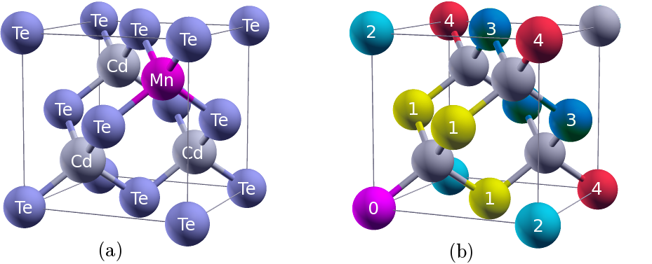
Figure 1: (a) Zn-blende structure for Cd_0.75Mn_0.25Te where one out of four Cd atoms is replaced by a Mn atom. (b) Positions of first, second, third, and fourth neighbors on the Cd fcc sub-lattice from the Cd atom in the lower left corner.

The spin of an isolated Mn ion aligns with any finite magnetic field. The non-trivial magnetization curves seen in experiment are due to the exchange interaction between different Mn ions. Test calculations confirmed that the interaction of three or more Mn ions is given by the sum of pair interactions so that we can concentrate on the interaction between pairs of Mn ions as a function of their distance. We found in numerically expensive calculations with $L=512$ atoms in the unit cell that the interaction between two Mn ions beyond 4th-neighbor distance is negligibly small. In Fig. 1(b) we show the first, second, third, and fourth neighbors on the fcc sublattice in CdTe.

II.1 GGA and GGA+$\bm{U}$ calculations

Ideally, we should study a single pair of Mn ions with Cd ions on all other sites of the cation fcc lattice. However, practical band-structure calculations require translational symmetry. Therefore, we start from large but finite cells with $L$ atoms that contain two Mn ions, and link them together so that periodic boundary conditions apply in all three spatial directions. Modern bandstructure program packages permit the investigation of large cells (‘supercells’). In this work, we use supercells with $L\leq 128$ atoms which are sufficiently large to study Mn pairs that are maximally fourth-nearest neighbors.

For our investigations we use the FLEUR package, FLE a high-precision implementation of the full potential linearized augmented planewave (FLAPW) approach to density-functional theory (DFT) in the generalized gradient approximation (GGA). The program package FLEUR also offers the option to include the effect of the correlations between the electrons in the partly filled $3d$-shell of the Mn ions on a mean-field level (GGA+$U$). In Sect. III, we compile results for the Mn-Mn interaction from both bandstructure approaches.

We run the FLEUR code using the following settings. We use the Generalized Gradient Approximation (GGA) functional of Perdew, Burke, and Ernzerhof Perdew et al. (1996) for the exchange-correlation energy. Since we are investigating a band insulator with a sizable gap, it is sufficient to use only 10 inequivalent ${\bf k}$-points in the irreducible part of the Brillouin zone; depending on the impurity positions, this corresponds to 20 or 40 ${\bf k}$-points in the full Brillouin zone. The basis functions inside the muffin tins are expanded in spherical harmonic functions with a cut-off of $L_{\rm max}=10$. The muffin tin radii are $R_{\rm Cd}=R_{\rm Mn}=2.64\,{\rm a.u.}$ and $R_{\mathrm{Te}}=2.58\,\mathrm{a.u.}$ ($1\,{\rm atomic\,unit}=a_{\rm B}=0.529\,\hbox{\AA}$). We use $R_{\rm Te}K_{\rm max}=8.26$, where $K_{\rm max}$ is the plane wave cut-off. For the GGA+$U$ calculations we use the standard double counting correction. Anisimov et al. (1997)

II.2 GGA+Gutzwiller approach

The electrons in the Mn ions’ $3d$ shell are strongly correlated. Therefore, more sophisticated many-particle techniques should be employed. For example, it would be desirable to use the fully self-consistent Gutzwiller-DFT. Schickling et al. (2014); Ho et al. (2008); Deng et al. (2009) At present, however, the required large unit cells prevent us from doing such a calculation and we restrict ourselves to a less costly method that is based on the evaluation of a Gutzwiller wave function for a tight-binding model with Hubbard-type interactions on the two Mn sites.

II.2.1 Derivation of the two-ion Hubbard model

The code Wannier90 permits a downfolding of the bandstructure to a tight-binding Hamiltonian in position space. Mostofi et al. (2008) We project onto a basis of $s$ orbitals and $p$ orbitals for each of the semiconductor atoms and $s$, $p$ and $d$ orbitals for the Mn impurity. However, the downfolding procedure is limited to $L=16$ atoms in the unit cell so that we cannot derive the tight-binding model for a pair of Mn ions directly.

To overcome this limitation, we assume that the combined influence of two Mn ions on the electron transfer between two lattice sites can be approximated by the linear superposition of the influence of two individual Mn ions. Under this linearity assumption, we are left with the investigation of a single Mn ion in a CdTe supercell of $L=16$ atoms. For our GGA calculations we use 120 ${\bf k}$-points in the irreducible part of the Brillouin zone (1/24 of the full Brillouin zone) and $R_{\mathrm{Te}}K_{\rm max}=9.80$.

First, we calculate the bandstructure for pure CdTe. The downfolding provides the tight-binding Hamiltonian for CdTe,

$$\hat{H}^{\rm CdTe}=\sum_{{\mathbf{i}},{\mathbf{j}},b_{1},b_{2},\sigma}t_{{\mathbf{i}},b_{1},\sigma}^{{\mathbf{j}},b_{2},\sigma}\hat{c}_{{\mathbf{i}},b_{1}\sigma}^{\dagger}\hat{c}_{{\mathbf{j}},b_{2}\sigma}^{\vphantom{\dagger}}\;,$$ (1)

where $\hat{c}_{{\mathbf{i}},b\sigma}^{\dagger}$ ($\hat{c}_{{\mathbf{i}},b\sigma}^{\vphantom{\dagger}}$) creates (annihilates) an electron in the orbital $b$ with spin $\sigma=\uparrow,\downarrow$. Due to the symmetry of our crystal, there are no local hybridization terms, and we may write

$$\hat{H}^{\rm CdTe} = \hat{T}^{\rm CdTe}+\hat{V}^{\rm CdTe}\;,$$

$$\hat{T}^{\rm CdTe} = \sum_{{\mathbf{i}}\neq{\mathbf{j}},b_{1},b_{2},\sigma}t_{{\mathbf{i}},b_{1},\sigma}^{{\mathbf{j}},b_{2},\sigma}\hat{c}_{{\mathbf{i}},b_{1}\sigma}^{\dagger}\hat{c}_{{\mathbf{j}},b_{2}\sigma}^{\vphantom{\dagger}}\;,$$

$$\hat{V}^{\rm CdTe} = \sum_{{\mathbf{i}},b,\sigma}t_{{\mathbf{i}},b,\sigma}^{{\mathbf{i}},b,\sigma}\hat{n}_{{\mathbf{i}},b\sigma}\;,$$ (2)

where $\hat{n}_{{\mathbf{i}},b\sigma}=\hat{c}_{{\mathbf{i}},b\sigma}^{\dagger}\hat{c}_{{\mathbf{i}},b\sigma}^{\vphantom{\dagger}}$ counts the number of electrons with spin $\sigma$ in orbital $b$ on site ${\mathbf{i}}$.

Next, we repeat the calculation with a single Mn ion at position ${\mathbf{f}}$ in the supercell which leads to a new set of electron transfer matrix elements $(t_{{\mathbf{i}},b_{1},\sigma_{1}}^{{\mathbf{j}},b_{2},\sigma_{2}})^{{\mathbf{f}}}$,

$$\hat{H}^{\rm CdTe,{\mathbf{f}}}=\sum_{{\mathbf{i}}\neq{\mathbf{j}},b_{1},b_{2},\sigma}(t_{{\mathbf{i}},b_{1},\sigma}^{{\mathbf{j}},b_{2},\sigma})^{{\mathbf{f}}}\hat{c}_{{\mathbf{i}},b_{1}\sigma}^{\dagger}\hat{c}_{{\mathbf{j}},b_{2}\sigma}^{\vphantom{\dagger}}+\hat{V}^{\rm CdTe}\;.$$ (3)

Due to periodic boundary conditions and the translational invariance of the crystal, the bands for CdTe with a single Mn ion do not depend on ${\mathbf{f}}$. The corresponding bands for pure CdTe and with a single Mn ion in the $L=16$ supercell are shown in Fig. 2.

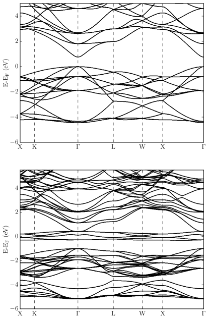
Figure 2: Band structures of CdTe (upper part of the figure) and of Cd_0.875Mn_0.125Te (lower part of the figure), calculated from a supercell with $L=16$ atoms without (with) a single Mn atom in the supercell using the FLEUR program package.

The upper part of the figure shows that the direct gap at the $\Gamma$-point is $E_{\rm sp}=0.76\,{\rm eV}$, in agreement with previous calculations. Wu et al. (2015) However, DFT(LDA) and DFT(GGA) underestimate the gap for the insulator CdTe. The (exciton) gap, a lower bound on the single-particle gap, is found at $E_{\rm xc}=1.5\,{\rm eV}$ for CdTe. Thomas (1961) DFT(GGA) also underestimates the charge-transfer gap in Mn-doped II-VI semiconductors between Te and Mn levels so that the resulting exchange couplings are too large, see Sect. III.1.1. The origin of the exchange coupling can be inferred from the lower part of Fig. 2. The Mn $3d$-bands are grouped around the Fermi energy so that they push down the CdTe bands that were below the gap, and hybridize at the $\Gamma$-point with a dominant Te-band above the CdTe gap. The band structure shows that the Mn-Te hybridization is responsible for the interaction between Mn ions.

To set up our Hamiltonian in the presence of two Mn impurities, we define the corrections to the electron transfer amplitudes

$$\bigl{(}\Delta_{{\mathbf{i}},b_{1},\sigma}^{{\mathbf{j}},b_{2},\sigma}\bigr{)}^{{\mathbf{f}}}=\bigl{(}t_{{\mathbf{i}},b_{1},\sigma}^{{\mathbf{j}},b_{2},\sigma}\bigr{)}^{{\mathbf{f}}}-t_{{\mathbf{i}},b_{1},\sigma}^{{\mathbf{j}},b_{2},\sigma}\;.$$ (4)

According to our linear superposition scheme, we model the presence of a second Mn impurity in our tight-binding Hamiltonian by adding independently the corrections for the first Mn ion at site ${\mathbf{f}}_{1}$ and the second impurity at site ${\mathbf{f}}_{2}$. This defines our tight-binding Hamiltonian for the two-site problem,

$$\hat{H}^{\rm tb} = \sum_{{\mathbf{i}}\neq{\mathbf{j}},b_{1},b_{2},\sigma}\bigl{(}t_{{\mathbf{i}},b_{1},\sigma}^{{\mathbf{j}},b_{2},\sigma}\bigr{)}^{{\mathbf{f}}_{1},{\mathbf{f}}_{2}}\hat{c}_{{\mathbf{i}},b_{1}\sigma}^{\dagger}\hat{c}_{{\mathbf{j}},b_{2}\sigma}^{\vphantom{\dagger}}+\hat{V}^{\rm CdTe}\;,$$

$$\bigl{(}t_{{\mathbf{i}},b_{1},\sigma}^{{\mathbf{j}},b_{2},\sigma}\bigr{)}^{{\mathbf{f}}_{1},{\mathbf{f}}_{2}} = \bigl{(}\Delta_{{\mathbf{i}},b_{1},\sigma}^{{\mathbf{j}},b_{2},\sigma}\bigr{)}^{{\mathbf{f}}_{1}}+\bigl{(}\Delta_{{\mathbf{i}},b_{1},\sigma}^{{\mathbf{j}},b_{2},\sigma}\bigr{)}^{{\mathbf{f}}_{2}}+t_{{\mathbf{i}},b_{1},\sigma}^{{\mathbf{j}},b_{2},\sigma}\;.$$ (5)

Our approximation neglects the joint influence of the impurities on the electron transfer matrix elements in their surrounding, in the spirit of standard alloy theory. Elliott et al. (1974) The supercells for the two-ion Hubbard model can be much larger than those used for its construction ($L=16$). For our further Gutzwiller calculations we work with cells containing $L=512$ atoms.

As a last step, we add the Hubbard interaction on the two Mn sites ${\mathbf{f}}_{1}$ and ${\mathbf{f}}_{2}$ and obtain the two-ion Hubbard model,

$$\hat{H} = \hat{H}^{\rm tb}+\hat{H}^{\rm loc}_{{\mathbf{f}}_{1}}+\hat{H}^{\rm loc}_{{\mathbf{f}}_{2}}+\hat{H}^{\rm dc}$$

$$\hat{H}^{\rm loc}_{{\mathbf{g}}} = \sum_{c_{1},\ldots,c_{4}=1}^{5}\sum_{\sigma.\sigma^{\prime}=\uparrow,\downarrow}U^{(c_{1}\sigma),(c_{2}\sigma^{\prime})}_{(c_{3}\sigma^{\prime}),(c_{4}\sigma)}$$

$$\hphantom{+\sum_{c_{1},\ldots,c_{4}=1}^{5}}\hat{c}_{{\mathbf{g}},c_{1}\sigma}^{\dagger}\hat{c}_{{\mathbf{g}},c_{2}\sigma^{\prime}}^{\dagger}\hat{c}_{{\mathbf{g}},c_{3}\sigma^{\prime}}^{\vphantom{\dagger}}\hat{c}_{{\mathbf{g}},c_{4}\sigma}^{\vphantom{\dagger}}\;,$$

$$\hat{H}^{\rm dc} = -E_{\rm dc}(\hat{n}_{{\mathbf{f}}_{1}}+\hat{n}_{{\mathbf{f}}_{2}})\;.$$ (6)

Here, $U^{.,.}_{.,.}$ describes the Coulomb interaction between the electrons in the $3d$-shell in the ten spin-orbit level $(c_{l}\sigma_{l})$ in either of the two Mn ions. Using some simplifying assumptions, all interaction coefficients can be expressed in terms of an intra-orbital Hubbard-$U$ and an inter-orbital Hund’s-rule $J$, Schickling et al. (2014) see Sect. III.

Lastly, $\hat{H}^{\rm dc}$ accounts for the double counting of interaction terms between the $3d$-electrons on a mean-field level, where $\hat{n}_{{\mathbf{g}}}=\sum_{c,\sigma}\hat{n}_{{\mathbf{g}},c\sigma}$ counts the number of correlated electrons on the Mn site ${\mathbf{g}}$. We use a particularly simple form for the double counting term. In essence, the choice of $E_{\rm dc}$ permits to fix the average number of electrons in the correlated Mn $3d$-orbitals and we shall present our results as a function of $n_{d}\equiv\sum_{c,\sigma}\langle n_{{\mathbf{f}}_{1},c,\sigma}\rangle=\sum_{c,\sigma}\langle n_{{\mathbf{f}}_{2},c,\sigma}\rangle$. Typically, we need $E_{\rm dc}\approx 20\,{\rm eV}$ to adjust $n_{d}\approx 5$.

II.2.2 Gutzwiller variational state

We approximate the true ground-state of our model Hamiltonian (6) by a Gutzwiller variational state,

$$|\Psi_{\rm G}\rangle=\hat{P}_{{\mathbf{f}}_{1}}\hat{P}_{{\mathbf{f}}_{2}}|\Phi_{0}\rangle\;,$$ (7)

where $|\Phi_{0}\rangle$ is the ground state of an (effective) single-particle Hamiltonian $H_{0}^{\rm qp}$, and $\hat{P}_{{\mathbf{g}}}$ is the single-site Gutzwiller correlator,

$$\hat{P}_{{\mathbf{g}}}=\sum_{\Gamma}\lambda_{\Gamma}\hat{m}_{{\mathbf{g}},\Gamma}$$ (8)

with ${\mathbf{g}}={\mathbf{f}}_{1},{\mathbf{f}}_{2}$. Here, $\hat{m}_{{\mathbf{g}},\Gamma}=|\Gamma\rangle_{{\mathbf{g}}}{}_{{\mathbf{g}}}\langle\Gamma|$ projects onto the atomic eigenstate $|\Gamma\rangle_{{\mathbf{g}}}$ of $\hat{H}^{\rm loc}_{{\mathbf{g}}}=\sum_{\Gamma}E_{\Gamma}\hat{m}_{{\mathbf{g}},\Gamma}$, and $\lambda_{\Gamma}$ are real variational parameters for each of the $2^{10}=1024$ states in the Mn $3d$-shell.

II.2.3 Gutzwiller approximation and energy minimization

To obtain the optimal values of the variational parameters $\lambda_{\Gamma}$ and the optimal single-particle product state $|\Phi_{0}\rangle$, we must minimize the energy functional

$$E^{\rm var}(\{\lambda_{\Gamma},|\Phi_{0}\rangle\})=\frac{\langle\Psi_{\rm G}|\hat{H}|\Psi_{\rm G}\rangle}{\langle\Psi_{\rm G}|\Psi_{\rm G}\rangle}\;.$$ (9)

We evaluate the expectation value in eq. (9) using the Gutzwiller approximation. Schickling et al. (2014) This corresponds to a neglect of correlations between the two Mn impurity sites.

Due to the presence of a second Mn impurity, the point group on each Mn site is not exactly cubic. Hence, the local density matrix for the correlated orbitals

$$C_{{\mathbf{g}},c\sigma,c^{\prime}\sigma}=\langle\Phi_{0}|\hat{c}_{{\mathbf{g}},c^{\prime}\sigma}^{\dagger}\hat{c}_{{\mathbf{g}},c\sigma}^{\vphantom{\dagger}}|\Phi_{0}\rangle$$ (10)

is not diagonal. However, the non-diagonal elements are very small, of the order of $10^{-3}$, and are therefore neglected in our calculations, i.e., we set

$$C_{{\mathbf{g}},c\sigma,c^{\prime}\sigma}=\delta_{c,c^{\prime}}n_{c,\sigma}\;.$$ (11)

For the same reason, we use the approximation that the matrix for the electron transfer renormalization is diagonal, $q_{c\sigma}^{c^{\prime}\sigma^{\prime}}=\delta_{c,c^{\prime}}\delta_{\sigma,\sigma^{\prime}}q_{c,\sigma}$. Then, the energy functional can be cast into the form Bünemann et al. (1998)

$$E^{\rm GA}(\{\lambda_{\Gamma},|\Phi_{0}\rangle\}) = \langle\Phi_{0}|\hat{T}|\Phi_{0}\rangle+\sum_{{\mathbf{i}},b,\sigma}t_{{\mathbf{i}},b,\sigma}^{{\mathbf{i}},b,\sigma}\langle\Phi_{0}|\hat{n}_{{\mathbf{i}},b\sigma}|\Phi_{0}\rangle$$ (12)

$$+\sum_{\Gamma}E_{\Gamma}\lambda_{\Gamma}^{2}\langle\Phi_{0}|(\hat{m}_{{\mathbf{f}}_{1},\Gamma}+\hat{m}_{{\mathbf{f}}_{2},\Gamma})|\Phi_{0}\rangle$$

$$-E_{\rm dc}\langle\Phi_{0}|\hat{n}_{{\mathbf{f}}_{1}}+\hat{n}_{{\mathbf{f}}_{2}}|\Phi_{0}\rangle\;,$$

where

$$\hat{T}=\sum_{{\mathbf{i}}\neq{\mathbf{j}},b_{1},b_{2},\sigma}q_{b_{1},\sigma}q_{b_{2},\sigma}\bigl{(}t_{{\mathbf{i}},b_{1},\sigma}^{{\mathbf{j}},b_{2},\sigma}\bigr{)}^{{\mathbf{f}}_{1},{\mathbf{f}}_{2}}\hat{c}_{{\mathbf{i}},b_{1}\sigma}^{\dagger}\hat{c}_{{\mathbf{j}},b_{2}\sigma}^{\vphantom{\dagger}}\;.$$ (13)

The $q$-factors depend on the variational parameters $\lambda_{\Gamma}$ and the local densities $n_{c,\sigma}$; explicit expressions can be found in Ref. [Schickling et al., 2014]. We include the Lagrange parameter $E_{\rm SP}$ for the normalization of $|\Phi_{0}\rangle$ and $\eta_{c,\sigma}$ to fulfill eq. (11). Then, the minimization of the energy functional (12) with respect to $\langle\Phi_{0}|$ leads to the effective single-particle problem Bünemann et al. (2012)

$$\hat{H}_{0}^{\rm qp}|\Phi_{0}\rangle = E_{\rm SP}|\Phi_{0}\rangle\;,$$

$$\hat{H}_{0}^{\rm qp} = \hat{T}+\sum_{{\mathbf{i}},b,\sigma}t_{{\mathbf{i}},b,\sigma}^{{\mathbf{i}},b,\sigma}\hat{n}_{{\mathbf{i}},b\sigma}$$ (14)

$$-\sum_{c,\sigma}(E_{\rm dc}+\eta_{c,\sigma})\Bigl{(}\hat{n}_{{\mathbf{f}}_{1},c\sigma}+\hat{n}_{{\mathbf{f}}_{2},c\sigma}\Bigr{)}\;.$$

The Lagrange parameters $\eta_{c,\sigma}$ are variational parameters that control the local spin density in the $3d$-levels on the Mn ions, while the double-counting energy $E_{\rm dc}$ determines the average number of Mn $3d$ electrons.

II.3 Exchange couplings

The notion of an ‘exchange coupling’ between the two Mn atoms hinges on the concept of a Heisenberg exchange between the two Mn impurity spins at ${\mathbf{f}}_{1}$ and ${\mathbf{f}}_{2}$,

$$\hat{H}_{\rm Heis}^{{\mathbf{f}}_{1},{\mathbf{f}}_{2}}=2J_{{\mathbf{f}}_{1}-{\mathbf{f}}_{2}}{\mathbf{S}}_{{\mathbf{f}}_{1}}\cdot{\mathbf{S}}_{{\mathbf{f}}_{2}}\;.$$ (15)

Here, we tacitly assume that the average filling of the $3d$-shell in the Mn atoms is close to integer filling, i.e., $n_{d}\approx 5$, and the Hund’s-rule coupling fixes the ground-state spin to $s=5/2$ on each ion. The exchange coupling is positive, $J_{{\mathbf{f}}_{1}-{\mathbf{f}}_{2}}>0$, for an antiferromagnetic coupling.

Under the assumption that a Heisenberg model provides an adequate description of the ground state (and low-energy excitations) of our two Mn impurities, we can estimate their exchange coupling using the bandstructure and GGA+Gutzwiller approach. We orient the Mn spins into the $z$-direction, either parallel (‘ferromagnetic alignment’) or antiparallel (‘Neél-antiferromagnetic alignment’). The algorithm converges to the corresponding (local) minima and provides $(\Delta E)_{{\mathbf{f}}_{1}-{\mathbf{f}}_{2}}=E_{\parallel}-E_{\perp}$ for the energy differences. This energy difference can also be calculated from the Heisenberg model (15),

$$(\Delta E)_{{\mathbf{f}}_{1}-{\mathbf{f}}_{2}} = 2J_{{\mathbf{f}}_{1}-{\mathbf{f}}_{2}}\langle{\rm FM}|{\mathbf{S}}_{{\mathbf{f}}_{1}}\cdot{\mathbf{S}}_{{\mathbf{f}}_{2}}|{\rm FM}\rangle$$ (16)

$$-2J_{{\mathbf{f}}_{1}-{\mathbf{f}}_{2}}\langle{\rm AFM}|{\mathbf{S}}_{{\mathbf{f}}_{1}}\cdot{\mathbf{S}}_{{\mathbf{f}}_{2}}|{\rm AFM}\rangle$$

$$= 4J_{{\mathbf{f}}_{1}-{\mathbf{f}}_{2}}(5/2)^{2}=25J_{{\mathbf{f}}_{1}-{\mathbf{f}}_{2}}\;,$$

with the spin states $|{\rm FM}\rangle=|5/2,5/2\rangle_{{\mathbf{f}}_{1}}|5/2,5/2\rangle_{{\mathbf{f}}_{2}}$ and $|{\rm AFM}\rangle=|5/2,5/2\rangle_{{\mathbf{f}}_{1}}|5/2,-5/2\rangle_{{\mathbf{f}}_{2}}$. Here we used that only the $z$-components contribute to the expectation values. In this way, the values $J_{{\mathbf{f}}_{1}-{\mathbf{f}}_{2}}=(\Delta E_{{\mathbf{f}}_{1}-{\mathbf{f}}_{2}})/25$ are accessible from approaches that employ itinerant electrons.

III Results

First, we show that the experimentally observed exchange couplings for Mn ion pairs up to 4th-neighbor distance can be reproduced from scaled DFT(GGA), GGA+$U$, and GGA+Gutzwiller. Second, we analyze the local occupancies as obtained from GGA+Gutzwiller.

III.1 Exchange couplings

The values for the exchange couplings $J_{n}$ in Cd(Mn)Te are known from experiment for up to 4th neighbors on the cation fcc lattice. The values for the couplings have been determined from the steps in the magnetization as a function of the externally applied field for very low temperatures, $T\lesssim 0.1\,{\rm K}$. Their sequence, e.g., the fact that $J_{4}>J_{2},J_{3}$, has been extracted from a fit of the data to cluster spin models. Bindilatti et al. Malarenko Jr. et al. (2000) find $J_{1}=6.1\pm 0.3\,{\rm K}$, $J_{2}=0.06\pm 0.01\,{\rm K}$, $J_{3}=0.18\pm 0.01\,{\rm K}$, and $J_{4}=0.39\pm 0.02\,{\rm K}$. In this section we derive and compare the exchange couplings from DFT(GGA), GGA+$U$ and GGA+Gutzwiller calculations, and compare the resulting magnetization curves with experiment.

$J$	$A^{a}_{a}$Exp.	GGA	s$\cdot$GGA	GGA+$U$	GGA+G
$A^{a}_{a}$$J_{1}$	6.1	17.1	6.1	6.1	6.1
$J_{2}$	00.06	0.30	0.11	0.10	0.10
$J_{3}$	00.18	0.96	0.34	0.30	0.27
$J_{4}$	00.39	1.44	0.51	0.49	0.61

Table 1: Heisenberg exchange couplings $J_{n}$ in K between Mn ions at $n$th neighbor distance on the Cd fcc lattice in CdTe from experiment, Malarenko Jr. et al. (2000) and from DFT(GGA), DFT(GGA) scaled by a factor $s=0.357$, GGA+$U$ for $\overline{U}=U-J=2.65\,{\rm eV}$, and GGA+Gutzwiller for $A=4.4\,{\rm eV}$, $B=0.1\,{\rm eV}$, $C=0.4\,{\rm eV}$ and $n_{d}=5.19$.

III.1.1 Coupling strengths

The DFT(GGA) calculation does not contain any specific parameters to adjust the exchange couplings. For large supercells, $L=128$, the influence of Mn pairs between neighboring supercells in negligibly small.

As seen from table 1, the value for the nearest-neighbor coupling from DFT(GGA) is too large by more than a factor of two, $J_{1}^{\rm DFT}=17.1\,{\rm K}\approx J_{1}/0.36$. DFT(GGA) overestimates the size of the exchange coupling because it finds a too small charge-transfer gap $\Delta_{\rm CT}$ between occupied Te levels and unoccupied Mn-levels in Cd(Mn)Te. In super-exchange models, Savoyant et al. (2014) the exchange integral $J_{1}$ is inversely proportional to $\Delta_{\rm CT}$ so that the exchange integral $J_{1}$ becomes too large in DFT(LDA) and DFT(GGA), by almost a factor of three. GGA+$U$ is frequently used to tackle gap problems in correlated insulators. When we apply a Hubbard-$U$ on the Mn sites, we find a larger charge-transfer gap which leads to smaller exchange couplings, see below. As mentioned in Sect. II.1, the gap in pure CdTe is too small in DFT(GGA) calculations. This can also be corrected using GGA+$U$. Wu et al. (2015) However, the exchange couplings between Mn ions are mediated by electron transfer processes between Mn and Te so that the precise value of the CdTe band gap is irrelevant for our considerations.

In Fig. 3 we show the dependence of $J_{1}^{{\rm GGA}+U}$ as a function of $U$ for various values of $J$. The exchange coupling only depends on the combination $\overline{U}=U-J$. Dudarev et al. (1998) For $\overline{U}=2.65\,{\rm eV}$ we obtain $J_{1}^{{\rm GGA}+U}=6.1\,{\rm K}$. The values for other exchange interactions for farther distances are collected in table 1. The values for $J_{2,3,4}^{{\rm GGA}+U}$ are very similar, and even slightly closer to experiment, than those from the scaled DFT(GGA). This demonstrates that an adjustment of the charge-transfer gap cures in effect the overestimation of the exchange interactions in DFT(GGA).

Lastly, we discuss the results for $J_{n}$ as obtained from our GGA+Gutzwiller calculations. We set $C=0.4\,{\rm eV}$, in agreement with crystal-field theory for data from infrared spectroscopy for isolated Mn²⁺ ions in CdTe. Jain (1991) Moreover, we use $C=4B$, i.e., $B=0.1\,{\rm eV}$, as is a reasonable assumption for transition metals. Sugano et al. (1970) A similar set of values was used in a recent study of exchange integrals in Mn-doped II-VI semiconductors. Savoyant et al. (2014) The Hubbard-parameter $U$ in transition metals is of the order of several eV. Aryasetiawan et al. (2006) In this work we set $A=4.4\,{\rm eV}$. Note that we have $U=A+4B+3C$ and $J=(5/2)B+C$ for our intra-orbital Hubbard interaction and Hund’s-rule coupling, or, for the Slater-Condon parameters, we have $F^{(0)}=A+(7/5)C$, $F^{(2)}=49B+7C$, and $F^{(4)}=(63/5)C$. Schickling et al. (2016) Therefore, our Hund’s-rule exchange on the Mn sites is $J=0.65\,{\rm eV}$ and we employ $F^{(0)}=4.96\,{\rm eV}$ or $U=6\,{\rm eV}$.

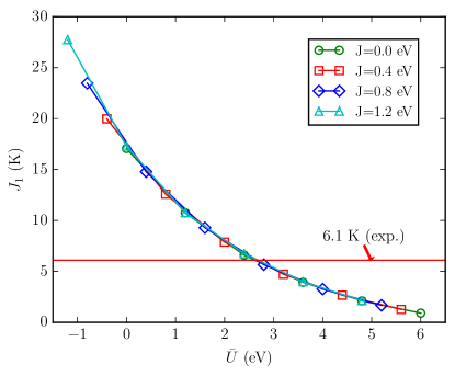
Figure 3: Heisenberg exchange coupling $J_{1}$ between two Mn ions in CdTe at nearest-neighbor distance from GGA+$U$ as a function of $\overline{U}=U-J$ calculated for a supercell with $L=128$ atoms using the FLEUR program package. The red horizontal line shows the experimental value $J_{1}^{\rm exp}=6.1\,{\rm K}$.

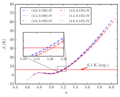
Figure 4: Heisenberg exchange coupling $J_{1}$ between two Mn ions in CdTe at nearest-neighbor distance from GGA+Gutzwiller as a function of the number of electrons in the Mn $3d$-shell for various values of the Racah parameters $A$, $B$, and $C=4B$. The red horizontal line shows the experimental value, $J_{1}^{\rm exp}=6.1\,{\rm K}$.

In Fig. 4, we show $J_{1}$ as a function of the electron number $n_{d}$ in the Mn $3d$-shell. As seen from the figure, the curves for $4.0\,{\rm eV}\leq A\leq 4.8\,{\rm eV}$ and $0.3\,{\rm eV}\leq C\leq 0.5\,{\rm eV}$ essentially collapse onto each other in the region of interest, $J_{1}=6.1\,{\rm K}$. Therefore, the specific choice of the Racah parameters is not crucial. As also seen from Fig. 4, the filling is not integer. Instead, we find that $n_{d}=5.19$ reproduces the nearest-neighbor Heisenberg exchange coupling best for $A=4.4\,{\rm eV}$, $B=0.1\,{\rm eV}$, $C=0.4\,{\rm eV}$. The resulting values for the exchange couplings for Mn ions in CdTe are compiled in table 1.

Our Gutzwiller calculations here are very close to a Hartree-Fock calculation. Correlation effects are small for the two fully polarized Mn atoms with their (anti-) parallel spins. We discuss this point further in Sect. III.2. This agreement is specific for Mn in II-VI semiconductors because we encounter a fully polarized, half-filled $3d$ shell in a wide-gap insulator. In other systems, correlation effects are more pronounced, as seen in some preliminary calculations for Cr-doped CdTe or Mn-doped GaAs.

For future reference, we compile the exchange couplings for Zn(Mn)Se, Zn(Mn)Te, and Zn(Mn)S in tables 4, 4, and 4. Note that the exchange couplings for $n>4$ are at least an order of magnitude smaller than $J_{2},J_{3}$, of the order of $J_{n\geq 5}=0.01\,{\rm K}$, or less. This justifies our restriction to $J_{n\leq 4}$.

As seen from the tables, the GGA+Gutzwiller method overestimates by some 20%-30% the nearest-neighbor exchange couplings $J_{1}$ for Zn-VI semiconductors (VI=Te, Se, S) when we use $A=4.4\,{\rm eV}$, $B=0.1\,{\rm eV}$, $C=0.4\,{\rm eV}$ and $n_{d}=5.19$ for the Mn ions. With this parameter set, the method can be used to provide a reasonable estimate for the nearest-neighbor couplings for Mn ion pairs in II-VI semiconductors. GGA+Gutzwiller provides a much better estimate for the couplings $J_{n\geq 2}$ than DFT(GGA) but they are still systematically too large by a factor two to three.

III.1.2 Magnetization for small doping and low temperatures

As an application, we calculate the magnetization $M(B)$ as a function of the applied external field $B$ for Cd_1-xMn_xTe at small but finite doping $x=0.005$. A Mn ion is placed in the center of a large but finite fcc lattice with $50^{3}$ sites. Then, Cd atoms in the surrounding of the ‘seed site’ are replaced by Mn atoms with probability $x$. As a first possibility, the central Mn ion remains isolated, i.e., with only Cd atoms on its 1st, 2nd, 3rd, and 4th neighbor shell (‘maximal surrounding’). In the absence of spin-orbit coupling, the spin of such an isolated Mn ion aligns with any finite magnetic field so that its magnetic response is given by the Brillouin function. Note that neglecting the spin-orbit coupling is justified because of the full magnetic polarization of the Mn ions. Bünemann et al. (2016)

A second possibility are two-spin clusters with exactly one Mn ion in the maximal surrounding of the seed site. Two such clusters are equivalent when they can be mapped onto each other by applying some space-group transformations of the fcc lattice. Since equivalent clusters lead to the same magnetic response we only need to store one representative $C$ and determine its multiplicity $A_{C}$. Moreover, we need to calculate the probability $p_{C}$ that a lattice point is part of cluster $C$. Liu et al. (1996); Bindilatti et al. (1998) For example, for a nearest-neighbor cluster we have $A_{C}=12$ and $p_{C}=x^{2}(1-x)^{72}$ (because in this case 72 sites must be unoccupied). This construction principle is readily generalized for clusters with three or more spins.

$J$	$A^{a}_{a}$Exp.	GGA	s$\cdot$GGA	GGA+G
$A^{a}_{a}$$J_{1}$	09.0	41.2	9.0	11.45
$J_{2}$	0.20	0.96	0.21	0.49
$J_{3}$	0.16	2.61	0.57	0.54
$J_{4}$	0.51	3.97	0.87	1.13

Table 2: Heisenberg exchange couplings $J_{n}$ in K between Mn ions at $n$th neighbor distance on the Zn fcc lattice in ZnTe from experiment, Bindilatti et al. (1998) from (scaled) DFT(GGA), and from GGA+Gutzwiller for $A=4.4\,{\rm eV}$, $B=0.1\,{\rm eV}$, $C=0.4\,{\rm eV}$ and $n_{d}=5.19$.

$J$	$A^{a}_{a}$Exp.	GGA	s$\cdot$GGA	GGA+G
$A^{a}_{a}$$J_{1}$	12.2	48.1	12.2	14.97
$J_{2}$	0.16	0.81	0.21	0.28
$J_{3}$	0.07	1.61	0.41	0.42
$J_{4}$	0.43	3.26	0.82	1.16

Table 3: Heisenberg exchange couplings $J_{n}$ in K between Mn ions at $n$th neighbor distance on the Zn fcc lattice in ZnSe from experiment, Bindilatti et al. (1998) from (scaled) DFT(GGA), and from GGA+Gutzwiller for $A=4.4\,{\rm eV}$, $B=0.1\,{\rm eV}$, $C=0.4\,{\rm eV}$ and $n_{d}=5.19$.

$J$	$A^{a}_{a}$Exp.	GGA	s$\cdot$GGA	GGA+G
$A^{a}_{a}$$J_{1}$	16.9	60.3	16.9	19.73
$J_{2}$	0.27	0.99	0.28	0.47
$J_{3}$	0.04	1.14	0.32	0.40
$J_{4}$	0.41	2.85	0.80	0.97

Table 4: Heisenberg exchange couplings $J_{n}$ in K between Mn ions at $n$th neighbor distance on the Zn fcc lattice in ZnS from experiment, Bindilatti et al. (1998) from (scaled) DFT(GGA), and from GGA+Gutzwiller for $A=4.4\,{\rm eV}$, $B=0.1\,{\rm eV}$, $C=0.4\,{\rm eV}$ and $n_{d}=5.19$.

In this work we include clusters with one to four Mn atoms and thus find in total 1130 inequivalent clusters $C$. At doping $x=0.005$, clusters with up to three Mn atoms cover 98.5% of all possible configurations, clusters with up to four Mn atoms cover 99.6% of all possible configurations. Therefore, clusters with five and more Mn atoms are irrelevant at $x=0.005$.

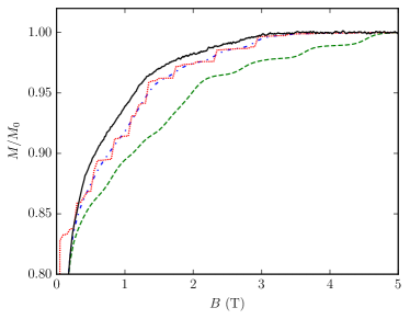
Figure 5: Magnetization $M(B)$ as a function of the external field $B$ normalized to its value at $B=5\,{\rm T}$ for Cd_1-xMn_xTe at Mn-doping $x=0.005$. Black line (solid): experimental curve; Malarenko Jr. et al. (2000) red line (dotted): Heisenberg model with experimental coupling parameters at $T=0$; blue line (dash-dotted): Heisenberg model with experimental coupling parameters at $T_{\rm spin}=0.1\,{\rm K}$; green line (dashed): Heisenberg model with GGA+Gutzwiller parameters at $T_{\rm spin}=0.1\,{\rm K}$. Clusters with up to four Mn ions are included.

For each cluster $C$, the interaction between the Mn spins is described by a Heisenberg model,

$$\hat{H}_{\rm Heis}^{C}(B)=\sum_{\begin{subarray}{c}{\mathbf{f}}_{1},{\mathbf{f}}_{2}\in C\\ ({\mathbf{f}}_{1}\neq{}{\mathbf{f}}_{2})\end{subarray}}J_{{\mathbf{f}}_{1}-{\mathbf{f}}_{2}}\hat{{\mathbf{S}}}_{{\mathbf{f}}_{1}}\cdot\hat{{\mathbf{S}}}_{{\mathbf{f}}_{2}}-g\mu_{\rm B}B\sum_{{\mathbf{f}}\in C}\hat{S}_{{\mathbf{f}}}^{z}\;,$$ (17)

where the sums run over all lattice sites ${\mathbf{f}}$ in cluster $C$, containing $n_{C}=1\ldots{}4$ spins. We include the interaction with the external field $B$ where $g=2$ is the gyromagnetic ratio and $\mu_{\rm B}$ is the Bohr magneton. For our comparisons with experiment, we use the experimental values for $J_{n}$ from table 1 and theoretical values from the GGA+Gutzwiller approach. However, the differences between scaled GGA, GGA+$U$, and GGA+Gutzwiller are fairly small.

For each cluster $C$, we determine its contribution to the magnetization per lattice site,

$$M^{C}(B)=\frac{1}{n_{C}}{\rm Tr}\Bigl{(}\hat{\rho}_{C}\sum_{{\mathbf{f}}\in C}\hat{S}_{{\mathbf{f}}}^{z}\Bigr{)}\;,\;\hat{\rho}_{C}=\frac{e^{-\beta\hat{H}^{C}_{\rm Heis}(B)}}{{\rm Tr}\bigl{(}e^{-\beta\hat{H}^{C}_{\rm Heis}(B)}\bigr{)}}$$ (18)

with $\beta=1/(k_{\rm B}T_{\rm spin})$. The trace is readily calculated using the exact spectrum that we obtain from a complete diagonalization of the cluster Hamiltonian $\hat{H}^{C}_{\rm Heis}(B)$. The magnetization per lattice site is then given by the sum over all clusters weighted by their multiplicity $A_{C}$ and probability $p_{C}$,

$$M(B)=\sum_{C}A_{C}{}p_{C}M^{C}(B)\;.$$ (19)

We show the resulting magnetization in Fig. 5.

The curve for zero temperature shows the expected magnetization steps that occur when more and more Mn pairs (or clusters) align with the external field. Foner et al. (1989) When we use the experimentally determined values for the exchange couplings from table 1 and a spin temperature $T_{\rm spin}=100\,{\rm mK}$ that is somewhat higher than the environment temperature $T=20\,{\rm mK}$, Malarenko Jr. et al. (2000) we find that the agreement between theory and experiment for $M(B)$ is very good. The agreement becomes slightly worse when we use the coupling parameters calculated by GGA+Gutzwiller. Note that the experimentally accessible magnetic fields probe mostly $J_{2}$, $J_{3}$ and $J_{4}$ because we have $k_{\rm B}T,g\mu_{\rm B}B\ll J_{1}$ and $k_{\rm B}T,g\mu_{\rm B}B\gg J_{n\geq 5}$.

III.2 Density and spin distributions

To gain further insight into the nature of the ground state of the Mn ion, we present results for the local occupancies.

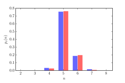
Figure 6: Mn charge distribution $p_{c}(n)$ as a function of the number $n$ of $3d$-electrons for $A=4.4\,{\rm eV}$, $B=0.1\,{\rm eV}$, $C=0.4\,{\rm eV}$ for $n_{d}=5.19$ in GGA+Gutzwiller (red columns), in comparison with the Hartree–Fock result (blue columns).

We start our discussion with the probability distribution $p_{c}(n)$ to find $n$ $3d$ electrons on the Mn ion on site ${\mathbf{f}}$ ($0\leq n\leq 10$). As seen from Fig. 6 the distribution peaks at $n=5$ which reflects the fact that the average particle number is $n_{d}=5.19$, see Sect. III.1.1. Correspondingly, there also is a sizable probability to find $3d^{6}$ configurations on the Mn ion whereas the probability for all other occupation numbers is negligible. Note that this distribution is not the result of electronic correlations because the corresponding Hartree–Fock state displays almost the same distribution function.

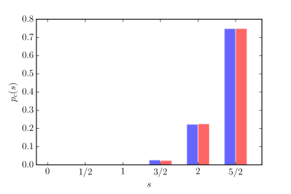
Figure 7: Mn spin distribution $p_{s}(s)$ as a function of the spin $s$ of $3d$-electrons for $A=4.4\,{\rm eV}$, $B=0.1\,{\rm eV}$, $C=0.4\,{\rm eV}$ for $n_{d}=5.19$ in GGA+Gutzwiller (red columns), in comparison with the Hartree–Fock result (blue columns).

The probability distribution function $p_{s}(s)$ for finding local spins with size $0\leq s\leq 5/2$ is very similar to the distribution in the single-particle product state $|\Phi_{0}\rangle$, i.e., the correlation enhancement of the local spin moment is also small for the spin distribution function, see Fig. 7. The average local spin is $\langle\hat{S}_{{\mathbf{f}}}^{z}\rangle_{\rm loc}=2.33$ because the admixture of spin $s=2$ to the dominant configurations with $s=5/2$ is not negligibly small.

The Mn ions do not show integer filling $n_{d}=5$, nor does the spin moment correspond to the atomic spin $s=5/2$. This observation puts into question the concept of a Heisenberg-model description that we employed in Sect. II.3 to derive the exchange couplings. Even if we accept a non-integer filling of the Mn ions’ $3d$-shell, we are actually far from a local-moment regime that is implicit in the Heisenberg-model description (15) in Sect. II.3. This issue can be resolved as seen in the next section.

IV Magnetic response of ion pairs at non-integer filling

In order to reconcile the finding of a non-integer Mn $3d$ filling and the notion of a spin $s=5/2$ effective Heisenberg model, we study the magnetic response in a simplified toy model of two Mn atoms close to their Hund’s rule ground states that are coupled to three uncorrelated sites. The uncorrelated sites serve two purposes, namely, (i), they act as a reservoir to adjust the average particle number on the Mn sites away from integer filling and, (ii), they serve as an intermediate charge-transfer (exchange) site to mimic the super-exchange mechanism.

IV.1 Model Hamiltonian

The Hamiltonian for our few-site toy-model, illustrated in Fig. 8, is readily formulated. We use the local Hamiltonian $\hat{H}_{{\mathbf{g}}}^{\rm loc}$ defined in eq. (6) for the Mn atoms at ${\mathbf{f}}_{\rm l}$ and ${\mathbf{f}}_{\rm r}$, and

$$\hat{H}_{\rm j}^{\rm loc}=\epsilon_{\rm j}\sum_{\sigma}\hat{n}_{{\rm j},\sigma}\;,$$ (20)

for the local Hamiltonians of the three uncorrelated orbitals. Here, $\epsilon_{\rm j}$ (${\rm j}={\rm l},{\rm e},{\rm r}$) are the local chemical potentials that permit the adjustment of the average electron number in the left (l) and right (r) bath orbitals and the exchange (e) orbital, and $\hat{n}_{{\rm j},\sigma}=\hat{c}_{{\rm j},\sigma}^{\dagger}\hat{c}_{{\rm j},\sigma}^{\vphantom{\dagger}}$ counts the number of electrons in the uncorrelated orbitals. The sites are coupled via the kinetic terms

$$\hat{T}_{{\rm l/e},{\mathbf{f}}_{\rm l}} = \sum_{c,\sigma}T_{{\mathbf{f}}_{\rm l},c,\sigma}^{{\rm l/e},\sigma}\hat{c}_{{\mathbf{f}}_{\rm l},c\sigma}^{\dagger}\hat{c}_{{\rm l/e},\sigma}^{\vphantom{\dagger}}+\hbox{h.c.}\;,$$

$$\hat{T}_{{\rm e/r},{\mathbf{f}}_{\rm r}} = \sum_{c,\sigma}T_{{\mathbf{f}}_{\rm r},c,\sigma}^{{\rm e/r},\sigma}\hat{c}_{{\mathbf{f}}_{\rm r},c\sigma}^{\dagger}\hat{c}_{{\rm e/r},\sigma}^{\vphantom{\dagger}}+\hbox{h.c.}\;.$$ (21)

The full model Hamiltonian reads

$$\hat{H} = \hat{H}_{{\mathbf{f}}_{\rm l}}^{\rm loc}+\hat{H}_{{\mathbf{f}}_{\rm r}}^{\rm loc}+\hat{H}_{\rm l}^{\rm loc}+\hat{H}_{\rm e}^{\rm loc}+\hat{H}_{\rm r}^{\rm loc}$$ (22)

$$+\hat{T}_{{\rm l},{\mathbf{f}}_{\rm l}}+\hat{T}_{\rm e,{\mathbf{f}}_{\rm l}}+\hat{T}_{\rm e,{\mathbf{f}}_{\rm r}}+\hat{T}_{{\rm r},{\mathbf{f}}_{\rm r}}\;.$$

The maximal dimension of the corresponding Fock space is ${\rm dim}H=1024^{2}\cdot 4^{3}$. It is too large to be handled exactly.

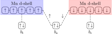
Figure 8: Toy model for the study of two Mn atoms with two reservoir sites and an indirect Mn-Mn coupling via a charge-transfer site.

From our analysis in Sect. III we know that, for large $U$, $J$, those Mn configurations are dominantly occupied that, in the sectors with $n_{d}=4,5,6$ electrons, have maximal spin $s_{\rm max}=2,5/2,2$ and maximal orbital momentum $l_{\rm max}=2,0,2$, which is a good quantum number in spherical approximation. Therefore, we restrict the Hilbert space of our two Mn atoms to these atomic subspaces. To this end, we introduce the projection operators ${\cal P}_{{\mathbf{g}},n_{d}}^{\rm H}$ onto the lowest-lying $(2s_{\rm max}+1)(2l_{\rm max}+1)$ Hund’s-rule states for fixed electron number $n_{d}$,

$$\hat{H}_{{\mathbf{g}}}^{\rm loc}|\Gamma_{n}\rangle_{{\mathbf{g}}} = E_{n}^{\rm loc}|\Gamma_{n}\rangle_{{\mathbf{g}}}\;,$$

$$\hat{n}_{{\mathbf{g}}}|\Gamma_{n}\rangle_{{\mathbf{g}}} = n_{d}|\Gamma_{n}\rangle_{{\mathbf{g}}}\;,$$

$$\hat{{\mathbf{S}}}_{{\mathbf{g}}}^{2}|\Gamma_{n}\rangle_{{\mathbf{g}}} = s_{\rm max}(s_{\rm max}+1)|\Gamma_{n}\rangle_{{\mathbf{g}}}\;,$$

$$\hat{{\mathbf{L}}}_{{\mathbf{g}}}^{2}|\Gamma_{n}\rangle_{{\mathbf{g}}} = l_{\rm max}(l_{\rm max}+1)|\Gamma_{n}\rangle_{{\mathbf{g}}}\;,$$

$${\cal P}_{{\mathbf{g}},n_{d}}^{\rm H} = \sum_{\Gamma_{n}}|\Gamma_{n}\rangle_{{\mathbf{g}}}\,{}_{{\mathbf{g}}}\langle\Gamma_{n}|\,.$$ (23)

Then, we define the total projection operator

$${\cal P}_{4,5,6}^{\rm H}=\left(\sum_{n_{d}=4}^{6}{\cal P}_{{\mathbf{f}}_{\rm l},n_{d}}^{\rm H}\right)\left(\sum_{n_{d}=4}^{6}{\cal P}_{{\mathbf{f}}_{\rm r},n_{d}}^{\rm H}\right)\;,$$ (24)

and we limit ourselves to the investigation of our model Hamiltonians in the projected form

$${\cal H}={\cal P}_{4,5,6}^{\rm H}\hat{H}{\cal P}_{4,5,6}^{\rm H}\;.$$ (25)

The dimension of the partial Fock space on the Mn atoms is $(2s_{\rm max}+1)(2l_{\rm max}+1)$ so that the maximal Fock-space dimension is ${\rm dim}{\cal H}=(25+6+25)^{2}\cdot 4^{3}=200704$. This partial Fock space is accessible using the Lanczos technique.

IV.2 Magnetization plateaus

The magnetic field couples to the spin-component of the Mn atoms in $z$-direction,

$$\hat{H}_{B}=-g\mu_{\rm B}B(\hat{S}_{{\mathbf{f}}_{\rm l}}^{z}+\hat{S}_{{\mathbf{f}}_{\rm r}}^{z})\;.$$ (26)

The magnetization is obtained from

$$M(B)=\langle\Psi_{0}|\hat{S}_{{\mathbf{f}}_{\rm l}}^{z}+\hat{S}_{{\mathbf{f}}_{\rm r}}^{z}|\Psi_{0}\rangle\;,$$ (27)

where $|\Psi_{0}\rangle$ is the ground-state of our model Hamiltonian in the presence of a magnetic field,

$${\cal H}(B)={\cal H}+\hat{H}_{B}\;.$$ (28)

We employ the Lanczos algorithm to find $|\Psi_{0}(B)\rangle$.

We fix the total number of electrons in the system to $n_{\rm tot}=16$, and choose the local chemical potentials $\epsilon_{\rm l}=\epsilon_{\rm r}$ to adjust the average electron number on the Mn sites so that we have an average number of $n_{d}=5.30$ electrons. Note that this number marginally changes as a function of the magnetic field. We set all electron transfer matrix equal in eq. (21), $T_{..}^{..}=1\,{\rm eV}$.

In the following case (i), we set $\epsilon_{\rm e}=8.0\,{\rm eV}$ and $\epsilon_{\rm l,r}=23.1\,{\rm eV}$ so that we have $n_{\rm e}=1.98$ electrons in the exchange orbital and $n_{\rm l,r}=1.71$ electrons in each bath orbital in the ground state. The resulting magnetization steps are equidistant, as shown in Fig. 9, despite the fact that the Mn filling is far from integer.

The width of the magnetization steps become non-uniform in case (ii) when the exchange site is not almost filled. To illustrate this case, we choose $\epsilon_{\rm e}=22.6\,{\rm eV}$ and $\epsilon_{\rm l,r}=19.5\,{\rm eV}$ so that we have $n_{\rm l,r}=1.93$ electrons in each bath orbital and $n_{\rm e}=1.51$ electrons in the exchange orbital. Now, the lengths of the corresponding magnetization plateaus are inequivalent, as shown in Fig. 10.

The toy model shows that equidistant plateaus are possible even though the occupation of the Mn sites is not integer. Our numerical observations can be readily understood using perturbative arguments. For negligible couplings to the exchange orbital, the ground state of each Mn ion and its attached bath site has spin $s=5/2$. Note that this spin is not solely located on the Mn site but also partly on the corresponding bath site. In case (i), the exchange orbital introduces only a small coupling between the left and the right spin-5/2 systems, and perturbation theory leads to a dominant term of the usual antiferromagnetic Heisenberg form (15). Consequently, the magnetization steps are equidistant. Larson et al. (1986); Foner et al. (1989) In case (ii), charge fluctuation contributions invalidate the simple spin-only picture. This results in non-equidistant magnetization steps as seen in Fig. 10.

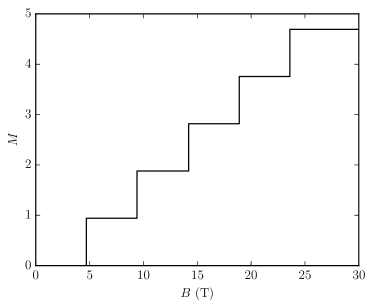
Figure 9: Magnetization $M(B)$ as a function of the external field for the toy model with an almost filled exchange site, $n_{\rm e}=1.98$.

When we apply the Gutzwiller approximation scheme used in Sect. III to case (i) of our toy model, we find an exchange coupling $J_{1}$ that is very close to the exact value derived from the width of the magnetization plateaus. This corroborates our finding in Sect. III and further justifies the applicability of our toy model.

Due to the large gap for charge excitations, the situation of Mn ions in CdTe resembles scenario (i) in our toy model and explains the experimental observation of equidistant magnetization plateaus. The filling of the Mn $3d$-shell is not integer but the total spin of the Mn ion and its surrounding atoms still is essentially $s=5/2$.

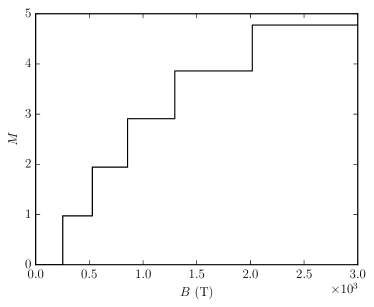
Figure 10: Magnetization $M(B)$ as a function of the external field for the toy model with a partly filled exchange site, $n_{\rm e}=1.51$.

V Conclusions

In this work we used three band structure methods, DFT(GGA), GGA+$U$, and GGA+Gutzwiller, to derive the exchange couplings between Mn ions diluted in II-VI semiconductor host materials such as CdTe. First, we calculate the energy of the configurations with parallel and antiparallel alignments of the Mn spins. Next, we interpret the energy difference in terms of a two-spin Heisenberg model and thereby deduce the exchange couplings as a function of the Mn-Mn separation for up to fourth neighbor distances.

For the GGA calculations we employ the FLEUR code with the functional of Perdew, Burke, and Ernzerhof for large supercells with $L=128$ atoms where two of the Cd ions are replaced by isovalent Mn ions. The ab-initio results for the exchange couplings are too large by a factor of two to three which is related to the fact that DFT(GGA) underestimates gaps in II-VI semiconductors systematically. The nearest-neighbor couplings $J_{1}$ for Mn ions in II-VI semiconductors can be reconciled with experiment by using the GGA+$U$ and GGA+Gutzwiller methods. These methods employ adjustable parameters that are used to match the experimental value for $J_{1}$ in Cd(Mn)Te. The exchange couplings $J_{2,3,4}$ for 2nd, 3rd, and 4th neighbor distances are then predictions from theory.

In general, the values for $J_{n\geq 2}$ agree qualitatively with experiment, i.e., band theory recovers $J_{4}>J_{2},J_{3}$ and $J_{n\geq 5}\lesssim 0.01\,{\rm K}$. However, the values for the couplings do not agree perfectly, i.e., we observe quantitative deviations up to a factor of two. About the same level of accuracy can be obtained by a simple rescaling of the DFT(GGA) data that fits the nearest-neighbor coupling $J_{1}$, see tables 1, 4, 4, and 4. The bare energy scale in our itinerant-electron description are of the order of several eV, i.e., of the order of $10^{5}\,{\rm K}$, whereas the exchange couplings $J_{n\geq 2}$ are one Kelvin and below. Therefore, it does not come as a surprise that the band structure methods reach their accuracy limits.

The notion of exchange couplings and the applicability of the super-exchange approach hinges on the mapping of the low-energy degrees of freedom of the itinerant-electron problem to those of a spin-5/2 Heisenberg model. This mapping successfully explains the equidistant magnetization plateaus as a function of applied magnetic field, as seen in experiment. However, the analysis of the Gutzwiller ground state for the two-ion Hubbard model shows that the filling of the Mn $3d$-shell is not integer which seemingly invalidates the whole concept of localized spins. The analysis of an exactly solvable few-site toy-model reassures that an integer filling is not a prerequisite for equidistant magnetization plateaus. Due to the hybridization of the Mn $3d$ orbitals with its insulating environment, a slightly delocalized spin-5/2 magnetic moment is formed combing Mn $3d^{5}$ and $3d^{6}$ with neighboring valence band states. Our picture of an extended spin-5/2 magnetic moment interacting with each other reconciles the usage of an effective spin-5/2 Heisenberg model to explain the experimentally observed magnetization steps and simultaneously a non-integer valence of the Mn 3d shell.

In the case of Mn-doped II-VI semiconductors, the Gutzwiller method and the Hartree-Fock approach to the two-ion Hubbard model lead to essentially the same results for an (anti-)ferromagnetic alignment of the Mn spins. Our preliminary investigations show that this is not the case for Cr in CdTe where the dopant electrons are more itinerant than in the case of Mn doping. We observe the same trend for Mn doping of GaAs and other III-V semiconductors. This observation also indicates that the Heisenberg mapping is less appropriate in these cases, and it is advisable to employ a correlated-electron approach for the description of the magnetic response in GaAs samples at low Mn doping.