Transport, shot noise, and topology in AC-driven dimer arrays

Abstract

We analyze an AC-driven dimer chain connected to a strongly biased electron source and drain. It turns out that the resulting transport exhibits fingerprints of topology. They are particularly visible in the driving-induced current suppression and the Fano factor. Thus, shot noise measurements provide a topological phase diagram as a function of the driving parameters. The observed phenomena can be explained physically by a mapping to an effective time-independent Hamiltonian and the emergence of edge states. Moreover, by considering quantum dissipation, we determine the requirements for the coherence properties in a possible experimental realization. For the computation of the zero-frequency noise, we develop an efficient method based on matrix-continued fractions.

Keywords: Quantum transport, time-dependent quantum systems, topology

1 Introduction

The ever smaller size of quantum dots implies small capacitances and accordingly large charging energies. Indeed in most recent realizations of coupled quantum dots, Coulomb repulsion represents the largest energy scale [1, 2] such that states with different electron numbers are energetically well separated. Then the quantum dot array can be controlled by gate voltages and, despite a possible coupling to electron reservoirs, the dynamics is restricted to a few states with a specific electron number. This forms the basis for many realizations of spin or charge qubits.

While quantum information processing is usually performed in closed systems, the possibility to couple quantum dots to electron source and drain may be useful as well. It not only can be exploited for qubit readout [3], but also allows one to determine the relevant system parameters. For example, upon increasing the source-drain bias, an increasing number of levels enters the voltage window such that a current measurement provides the spectrum of the coupled quantum dots. The dominating feature in the current-voltage profile is provided by the mentioned charging effects which cause Coulomb blockade. Further blockade mechanisms come about when in addition spin effects [4] or phononic excitations [5, 6, 7] play a role. Moreover, in a dimer chain, the interplay of Coulomb interaction and the topology may cause edge-state blockade [8]. It is particularly visible in the shot noise properties of the transport process.

Experimental evidence for edge-state blockade will be facilitated by a high tunability of the inter-dot tunneling. A possible way to circumvent this problem is driving the conductor by an electric dipole field. Then for not too small frequencies, the driving essentially renormalizes the inter-dot tunnel coupling [9, 10, 11, 12] and, thus, allows the emulation of a dimer chain with highly tunable tunneling. In the corresponding transport setting, i.e., in the presence of electron source and drain, one expects a corresponding current suppression [13, 14] which has been measured in double quantum dots [15, 16]. Moreover, the driving may have significant impact on the shot noise [17]. In this work, we explore the possibility for edge-state blockade in ac driven quantum dot arrays such as those sketched in Fig. 1. It is based on the recent finding that the topological properties of ac driven dimer chains can be controlled via the amplitude of a driving field [18, 19, 20].

In the regime of strong Coulomb repulsion and relatively small dot-lead tunneling, an established way to describe transport are master equations of the Bloch-Redfield type [21, 22, 23]. In combination with a Floquet theory for the central system, they can be applied to periodically driven transport problems including to the computation of shot noise [14]. The computation of the required dissipative kernels, however, may be numerically demanding. In certain limits, however, the master equation assumes a convenient Lindblad form which is easier to evaluate. For its efficient numerical treatment, we extend a previously developed matrix-continued fraction method [24] to the computation of shot noise.

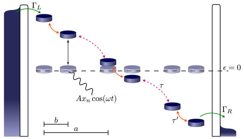
Figure 1: Dimer chain with intra-dimer tunnel coupling $\tau^{\prime}=\tau_{0}-\delta\tau$ and inter dimer coupling $\tau=\tau_{0}+\delta\tau$, connected to the electron source (left) and drain (right) with rate $\Gamma_{L,R}$. The applied external AC field generates an oscillation of the onsite energies with frequency $\omega$ which depends on the positions of the quantum dots, $x_{n}$, therefore the inter and intra dimer distances, $a$ and $b$ respectively, become relevant even for the tight-binding description.

This work is structured as follows. In Sec. 2, we introduce our model and a master equation description, as well as a matrix-continued fraction method for the computation of the current and the zero-frequency noise of time-dependent transport problems. The main features of the current are presented in Sec. 3, while Sec. 4 is devoted to the impact of dissipation. In the A, we test an assumption made for the efficient computation of the Fano factor.

2 Model and master equation

We consider an array of quantum dots coupled to a time-dependent electric dipole field such that the onsite energies oscillate in time with a position-dependent amplitude, see Fig. 1. The static part is given by the Su-Schrieffer-Heeger (SSH) Hamiltonian [25]

$$H_{\mathrm{SSH}}=\sum_{n=1}^{N-1}\tau_{n}c_{n+1}^{\dagger}c_{n}+\mathrm{h.c.},$$ (1)

where $c_{n}$ is the fermionic annihilation operator for an electron on site $n$ located at position $x_{n}$. We will focus on a dimer chain with an even number of sites, $N$, and alternating tunnel matrix elements $\tau_{n}=\tau_{0}+(-1)^{n}\delta\tau$. The AC field couples via the dipole operators of the chain such that the Hamiltonian of the driven chain reads

$$H(t)=H_{\mathrm{SSH}}+A\sum_{n=1}^{N}x_{n}c_{n}^{\dagger}c_{n}\cos(\omega t)$$ (2)

with $x_{n}$ the position of site $n$. The distances between two neighboring sites are $b$ and $a-b$, which implies a unit cell of length $a$. The driving is determined by its frequency $\omega$ and amplitude $A$.

2.1 Generalized chirality

The topological properties of the SSH model stem from a chiral (or sub-lattice) symmetry $C$ with $CH_{\mathrm{SSH}}C=-H_{\mathrm{SSH}}$. In second quantization, this symmetry operation can be written as

$$C=e^{\pi i\sum_{n}nc_{n}^{\dagger}c_{n}}=C^{-1}.$$ (3)

In essence, it provides a minus sign for all creation and annihilation operators with an odd site number since

$$Cc_{n}C=(-1)^{n}c_{n}.$$ (4)

Consequently, all nearest-neighbor hoppings acquire a factor $-1$ which explains the mentioned chiral symmetry of $H_{\mathrm{SSH}}$. The time-dependent part of the Hamiltonian (2) consists of local terms $c_{n}^{\dagger}c_{n}$ which are invariant under transformation with $C$. However, the sinusoidal driving allows us to obtain a minus sign via shifting the time by half a driving period, $t\to t+T/2$, where $T=2\pi/\omega$. Formally, this can be expressed as

$$CH(t)C=-H(t+T/2).$$ (5)

We refer to this symmetry relation as “generalized chirality”, owing to its resemblance to the generalized parity present in symmetric bistable potentials driven by a dipole force [9].

A consequence of the generalized chirality is that the propagator of the chain, $U(t,t^{\prime})$, obeys the relation

$$U(t+T,t+T/2)=CU^{-1}(t+T/2,t)C.$$ (6)

Thus, the one-period propagator can be split in two symmetry-related parts, a fact that has been identified as a condition for non-trivial topological properties of a periodically driven system [26].

2.2 Counting statistics

Transport is enabled by coupling the first and the last site to an electron source and drain, respectively. In the limit in which the applied voltage is much larger than the tunnel matrix elements $\tau_{n}$, but still considerably smaller than the Coulomb repulsion of the electrons on the array [8], a standard Bloch-Redfield approach to second order in the chain-lead tunneling provides the Lindblad master equation

$$\dot{\rho}=\mathcal{L}\rho=-\frac{i}{\hbar}[H(t),\rho]+\Gamma_{L}\mathcal{D}(c_{1}^{\dagger})\rho+\Gamma_{R}\mathcal{D}(c_{N})\rho,$$ (7)

with $\mathcal{D}(x)\rho=(2x\rho x^{\dagger}-x^{\dagger}x\rho-\rho x^{\dagger}x)/2$ and the dot-lead rates $\Gamma_{L,R}$. In the limit considered, Eq. (7) has to be evaluated in the basis with at most one electron on the array. This restricted basis captures Coulomb interaction.

To compute the statistics of the transported electrons, we have to generalize the master equation by introducing a counting variable $\chi$ for the electrons in the right lead. Proceeding as in Ref. [8], we consider the generalized reduced density operator $R_{\chi}$ which for the present case of uni-directional transport obeys the equation of motion [27]

$$\dot{R}_{\chi}(t)=\left[\mathcal{L}+(e^{i\chi}-1)\mathcal{J}\right]R_{\chi}(t)\,.$$ (8)

It is defined such that the moment-generating function of the electron number in the right lead, $N$, becomes $\langle e^{i\chi N}\rangle=\tr R_{\chi}$ and, thus, $\langle N^{k}\rangle_{t}=(\partial/i\partial\chi)^{k}\tr R_{\chi}(t)|_{\chi=0}$. Taylor expansion of $R_{\chi}$ in $\chi$ as

$$R_{\chi}(t)=F_{0}(t)+\sum_{k=1}^{\infty}\frac{(i\chi)^{k}}{k!}F_{k}(t)$$ (9)

relates the $F_{k}$ to the moments $\langle N^{k}\rangle_{t}=\tr F_{k}(t)$. Inserting this decomposition into the generalized master equation (7), provides the hierarchy

$$\dot{F}_{0} = \mathcal{L}F_{0}\,,$$ (10)

$$\dot{F}_{1} = \mathcal{L}F_{1}+\mathcal{J}F_{0}\,,$$ (11)

$$\dot{F}_{2} = \mathcal{L}F_{2}+\mathcal{J}F_{0}+2\mathcal{J}F_{1}\,.$$ (12)

Obviously, the first equation is the original master equation (7) and $F_{0}=\rho$.

For typical Markovian and time-independent transport problems, the cumulants eventually grow linearly in time, which motivates us to focus on the time-derivatives $\tr\dot{F}_{k}=(d/dt)\langle N^{k}\rangle$. To obtain the current expectation value, we solve Eq. (10) and insert the solution into Eq. (11) which yields $I(t)=\tr\dot{F}_{1}=\tr\mathcal{J}F_{0}$. The second moment follows from Eq. (12) together with the solution of the first two equations. Subtracting the time-derivative of $\langle N\rangle^{2}$, we obtain the zero-frequency noise

$$S(t)=\frac{d}{dt}\left[\tr F_{2}-(\tr F_{1})^{2}\right]=I(t)+2\tr\mathcal{J}F_{1\perp}\,,$$ (13)

where $F_{1\perp}=F_{1}-F_{0}\tr F_{1}$ represents the component of $F_{1}$ perpendicular to $F_{0}$. It obeys the equation of motion

$$\dot{\mathcal{F}}_{1\perp}=\mathcal{L}\mathcal{F}_{1\perp}+\left(\mathcal{J}-I(t)\right)F_{0}\ .$$ (14)

Notice that this equation depends on the current expectation value $I(t)$ and, thus, on the solution of the master equation (7).

2.3 Matrix-continued fractions

A natural way to solve Eqs. (7) and (14) is the numerical integration of the first equation followed by the computation of $I(t)$ and the numerical integration of the second equation. While being very flexible, such numerical propagation schemes often lack efficiency. Therefore we aim at implementing a matrix-continued fraction method [28] which in the context of mesoscopic transport has been employed recently for the computation of time-averaged currents [24]. Here we extend this scheme to the computation of the zero-frequency noise.

For convenience, we write the two equations of motion in block matrix notation,

$$\left(\begin{array}[]{c}\dot{\rho}\\ \dot{{\cal F}}_{1\perp}\end{array}\right) = \left(\begin{array}[]{cc}{\cal L}(t)&0\\ {\cal J}-I(t)&{\cal L}(t)\end{array}\right)\left(\begin{array}[]{c}\rho\\ {\cal F}_{1\perp}\end{array}\right)$$ (21)

$$\equiv M(t)\mathbf{b}$$ (22)

with the shorthand notation $\mathbf{b}=(\rho,\mathcal{F}_{1\perp})^{T}$. To derive a matrix-continued fraction scheme, we have to bring this equation into the form of a tridiagonal recurrence relation [28]. In the present case, this is hindered by the fact that $M(t)$ depends on the time-dependent current $I(t)$ which may contain higher-order harmonics. Here however, we find that reliable results for the noise can still be obtained when $I(t)$ is replaced by its time average. We test this assumption in A. Since now the remaining time-dependence in $M(t)$ stems from the Liouvillian of the sinusoidal driving in the Hamiltonian (2), the Fourier decomposition of the terms in Eq. (22) reads

$$M(t) = M_{0}+M_{+}e^{i\omega t}+M_{-}e^{-i\omega t},$$ (23)

$$\mathbf{b}(t) = \sum_{n=-\infty}^{\infty}e^{in\omega t}\mathbf{b}_{n}.$$ (24)

By inserting Eq. (24) into Eq. (22) we obtain the tridiagonal recurrence relation

$$M_{+}\mathbf{b}_{n-1}+\left(M_{0}-in\omega\right)\mathbf{b}_{n}+M_{-}\mathbf{b}_{n+1}=0\,.$$ (25)

Our interest lies in the time-average of $\mathbf{b}(t)$, i.e., in the Fourier component $\mathbf{b}_{0}$. To this end, we define the transfer matrices $S_{k}$ and $R_{k}$ via the ansatz

$$\mathbf{b}_{n}=\cases{R_{n}\mathbf{b}_{n+1}&for $n<0$ ,\\ S_{n}\mathbf{b}_{n-1}&for $n>0$ .}$$ (26)

Consistency with Eq. (25) is ensured by the recurrence relations

$$S_{n}={} -\left[M_{0}-in\omega+M_{-}S_{n+1}\right]^{-1}M_{+},$$ (27)

$$R_{n}={} -\left[M_{0}-in\omega+M_{+}R_{n-1}\right]^{-1}M_{-},$$ (28)

together with

$$(M_{0}+M_{+}R_{-1}+M_{-}S_{1})\mathbf{b}_{0}=0.$$ (29)

For practical purposes, we have to truncate the Fourier components of $\mathbf{b}(t)$ assuming $\mathbf{b}_{n}=0$ for $|n|>n_{0}$ which holds for $S_{n_{0}+1}=R_{-(n_{0}+1)}=0$. With the latter condition we compute $R_{-1}$ and $S_{1}$ by iterating Eqs. (27) and (28) which finally provides an explicit expression for Eq. (29). In a last step we solve this homogeneous equation under the trace conditions $\tr\rho_{0}=1$ and $\tr\mathcal{F}_{1\perp}=0$.

3 Transport in the high-frequency regime

The main energy scale of the SSH Hamiltonian (1) is the bandwidth $\tau_{0}$. If it is much smaller than the energy quanta of the driving field, $\hbar\omega$, one may employ a high-frequency approximation to derive an effective time-independent Hamiltonian that captures the long-time-dynamics of the driven system. This typically results in an effective Hamiltonian with parameters renormalized by Bessel functions. In this way, the AC-driving offers a possibility for tuning system parameters. A classic example is the suppression of tunneling in bistable potentials [9, 10] and superlattices [11, 29] by the purely coherent influence of an ac field.

In a dimer chain driven by an external electric field, the intra and inter dimer spacings become relevant because they determine the dipole moments and, thus, appear in the renormalizations of the inter dimer tunneling $\tau$ and the intra-dimer tunneling $\tau^{\prime}$ which in our case read

$$\tau_{\mathrm{eff}}^{\prime} = J_{0}(Ab/\omega)(\tau_{0}-\delta\tau),$$ (30)

$$\tau_{\mathrm{eff}} = J_{0}(A(a-b)/\omega)(\tau_{0}+\delta\tau),$$ (31)

where $J_{0}$ is the zeroth-order Bessel function of the first kind. For details of the calculation, see Ref. [18]. With these effective tunnel matrix elements, one can draw conclusions about the topological properties of the chain by a comparison with results for the time-independent SSH model [30, 31]. The main finding is a trivial topology for $\tau_{\mathrm{eff}}^{\prime}>\tau_{\mathrm{eff}}$, while for $\tau_{\mathrm{eff}}^{\prime}<\tau_{\mathrm{eff}}$ it becomes non-trivial with a Zak phase $\pi$ [18, 19]. Similar influence of radiation on topology occurs also in higher dimensions [32, 33, 34].

The tunnel matrix elements (30) and (31) possess an interesting duality. By the replacement $(\delta\tau,b)\to(-\delta\tau,a-b)$, these matrix elements are interchanged. Then the topological properties are interchanged as well, while the bulk spectra remain the same. This motivated the choice of parameters used in Fig. 2.

3.1 Current suppression and edge-state blockade

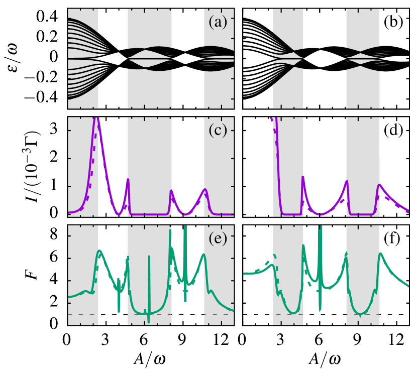
Figure 2: (a,b) Quasienergy spectrum as a function of the driving amplitude $A$ for (a) $\delta\tau=0.2\tau_{0}$, $b=0.4a$ and (b) $\delta\tau=-0.2\tau_{0}$, $b=0.6a$ for a chain with $N=20$ sites. The parameters are chosen such that the bulk spectra in the thermodynamic limit are identical, while the topological properties depend on the sign of $\delta\tau$. Accordingly, we find edge-states at zero quasienergies in the regions marked by a grey background. (c,d) Time-averaged current. The dashed lines correspond to the high-frequency approximation result. The driving frequency is $\omega=5\tau_{0}$, while the chain-lead coupling reads $\Gamma=5\tau_{0}$. (e,f) Fano factor $F=\bar{S}/\bar{I}$.

If the driving amplitude $A$ is such that one of the Bessel functions in Eqs. (30) and (31) vanishes, the way from the electron source to the drain is practically interrupted, which significantly reduces the current. The data in Fig. 2 confirm this expectation and reveal a particular dependence on topology: It is best visible in a comparison of data for two parameter sets that are related by the transposition of inter-dot and intra-dot coupling (left and right column, respectively, of this figure). Both choices lead to the same bulk properties, while the topological and the trivial regions are interchanged. This allows us to identify topological effects. The complementarity of the two cases is evident from the quasienergy spectra shown in Figs. 2(a) and 2(b).

Figures 2(c) and 2(d) show a remarkable dependence of the current suppression on the topology. In the trivial region, the current is extensively reduced only when the effective inter dimer tunneling vanishes, i.e., for $\tau_{\mathrm{eff}}\ll\tau_{0}$ [$A\approx 9\omega$ in Fig. 2(c) and $A\approx 6\omega$ in Fig. 2(d)]. Close to the suppression, the current grows quadratically, such as for a driven double quantum dot [14]. By contrast, the current almost vanishes in the whole topological region, i.e., whenever the weaker condition $\tau_{\mathrm{eff}}^{\prime}<\tau_{\mathrm{eff}}$ is fulfilled. Therefore, we can conclude that the physical origin of this current suppression is not a completely vanishing effective tunnel matrix element, but must be related to topology and the corresponding edge states formed at the source and at the drain. These edge states possess two characteristic features. First, they are exponentially weakly connected and, second, they are energetically well separated from the bulk states. As a consequence, they may trap electrons and thereby interrupt the transport process such that one observes edge-state blockade. As compared to its counterpart in time-independent chains [8], this blockade is characterized by a broad region with vanishing current, while the CDT-like suppression of current in the trivial region has a parabolic shape.

3.2 Shot noise and phase diagram

For less tunable static chains, it has been proposed to identify edge-state blockade by its characteristic shot noise properties [8]. In particular, it has been found that the small current in the blockade regime obeys Poissonian statistics ($F\approx 1$), while the transport in the trivial regime is characterised by electron bunching [35, 36]. Figures 2(e) and 2(f) depict the shot noise for the driven case characterized by the Fano factor. It reveals a smeared crossover between Poissonian noise and super Poissonian values up to $F\approx 8$.

The difficulty of performing an experiment on a chain with many sites raises the question about the necessary length to observe the edge state blockade. Thus we have calculated the Fano factor corresponding to the parameters in Fig. 2(f) for chains of different length. An advantage of using the external AC field to manipulate the topological phase is that the ideal Poissonian Fano factor $F\approx 1$ is always reached for a certain point in the blockade region, as shown in Fig. 3. This finding is in contrast to the static case, where $F\approx 1$ was found only in the limit of very long chains [8]. However, Fig. 3 also shows that for a short chain the Fano factor in the CDT point also approaches unity, which does not allow distinguishing the CDT effect from the topological blockade.

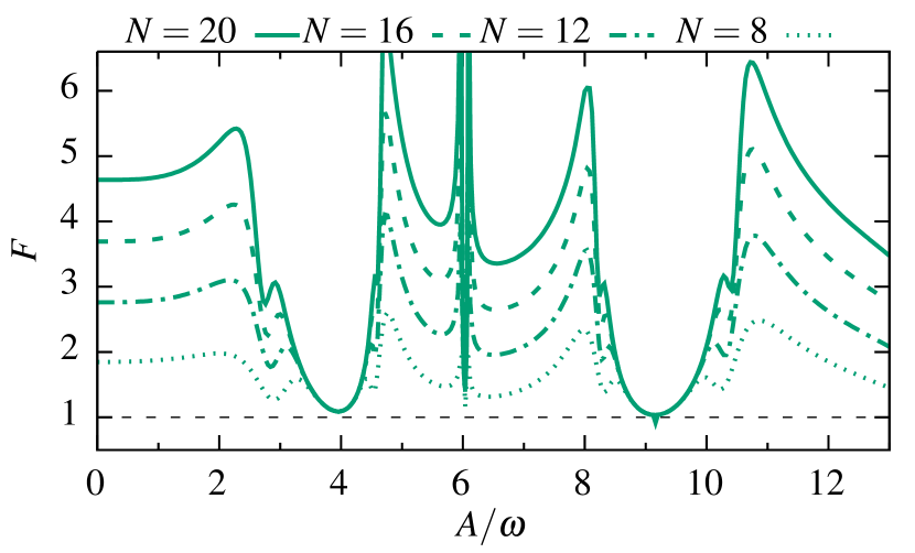
Figure 3: Fano factor $F=\bar{S}/\bar{I}$ as a function of the driving amplitude $A$ for $\delta\tau=-0.2\tau_{0}$, $b=0.6a$ for chains of various lengths. The driving frequency and the lead-chain coupling are $\omega=5\tau_{0}$ and $\Gamma=5\tau_{0}$, respectively.

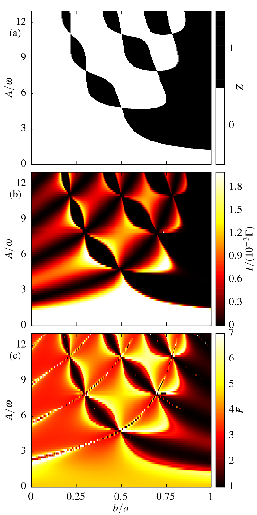
Figure 4: (a) Chern number as calculated in Ref. [18] as a function of the intra dimer distance $b$ and the driving amplitude $A$. All other parameters are as in the right column of Fig. 2. (b) Corresponding time-averaged current and (c) Fano factor.

While in contrast to the static case [8], here the shape of the current suppression may be sufficient to identify edge-state blockade, it will turn out that the Fano factor exhibits clearer fingerprints of the topological phase diagram computed as in Ref. [18] and shown in Fig. 4(a). The corresponding plot for the current [Fig. 4(b)] exhibits a richer structure stemming from the additional current suppressions in the trivial regions. Therefore the behavior of the current alone does not reflect the topological phase. The Fano factor [Fig. 4(c)], by contrast, provides clearer evidence, because $F\approx 1$ is found exclusively for non-trivial topology (black regions). We also find some additional structure in the trivial region as narrow lines at CDT-like zeros of the current. There, the Fano factor assumes even larger values which correspond to the sharp peaks in Figs. 2(e) and 2(f). Thus, shot noise measurements represent an alternative to the direct observation of the Zak phase [37].

4 Quantum dissipation

In Ref. [8], we have shown that for the static SSH model, the fingerprints of the topological properties in the Fano factor are fairly insensitive to weak static disorder. In the non-trivial region, the edge state formation is even supported by disorder and, thus, the Fano factor remains at the Poisson level. In the trivial region, we witnessed a slightly increased Fano factor.

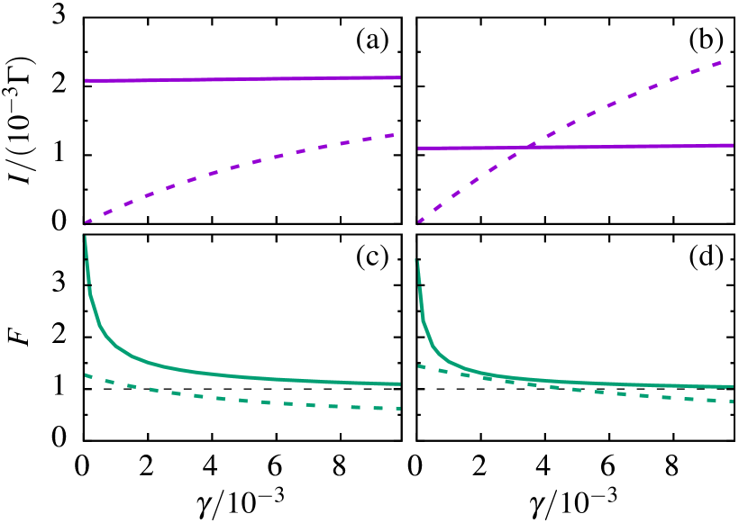
Figure 5: Influence of dissipation. (a,b) Time-averaged currents and (c,d) corresponding Fano factors as a function of the dissipation rate $\gamma$ for the amplitudes $qE/\omega=3.5$ and $qE/\omega=7$. The left and right column corresponds to the respective column of Fig. 2, i.e., (a,c) $\delta\tau=0.2\tau_{0}$ and $b=0.4a$, while (b) and (d) correspond to the complementary case $\delta\tau=-0.2\tau_{0}$ and $b=0.6a$. Solid lines mark topologically trivial cases, while dashed lines correspond to non-trivial topology. The driving frequency is $\omega=5\tau_{0}$, while the chain-lead coupling reads $\Gamma=5\tau_{0}$.

Here we investigate the impact of a dynamic disorder stemming from the interaction of each site with a respective heat bath via the population operators $c_{n}^{\dagger}c_{n}$. For weak coupling, we use a simple description with a Lindblad operator [23] with equal coupling strengths and modify the Liouvillian according to

$$\mathcal{L}\to\mathcal{L}+\gamma\sum_{n}\mathcal{D}(c_{n}^{\dagger}c_{n}),$$ (32)

where $\mathcal{D}$ is the Lindblad form defined after Eq. (7).

Figures 5(a) and 5(b) depicts how the current changes upon increasing the dissipation strength for two selected driving amplitudes. We focus on the two complementary parameter sets used in Fig. 2 and select two particular driving amplitudes, one corresponding to trivial topology (solid lines), the other to non-trivial topology (dashed lines). For trivial topology, the current is rather insensitive to weak dissipation. The main reason for this is that in the trivial region, the transport occurs via the delocalized eigenstates of the chain while coherences between these states play a minor role [8]. Accordingly, decoherence is not a relevant issue. For non-trivial topology, by contrast, the current grows with an increasing dissipation strength $\gamma$. A physical picture for this behavior is the direct transport between edge states. Since the splitting of the edge state doublet is exponentially small, the current is rather weak. Then dissipative transitions turn out to be rather beneficial for the electron transport.

In contrast to the current, shot noise is affected by dissipation in the same way as can be appreciated in Figs. 5(c) and 5(d). For both trivial and non-trivial topology, dissipation reduces the Fano factor which soon assumes value close to the Poissonian $F=1$. This means that measuring the topological phase diagram via the Fano factor (see Fig. 4) will require samples with very good coherence properties such that $\gamma\lesssim 10^{-3}\tau_{0}$, a value that seems feasible with present quantum dot technology [16].

5 Conclusions

We have investigated the influence of an AC driving on the current through a SSH chain whose first and last site is coupled to an electron source and drain, respectively. Owing to their topological properties and the corresponding presence of edge states, such chains have potential applications in quantum information processing. In the present case the topological properties can be controlled in a very flexible manner via driving frequency and amplitude. In topologically non-trivial parameter regions, edge states emerge and significantly influence the Fano factor of the current. In turn, the Fano factor may be used to measure the topological phase diagram.

For the computation of the shot noise, we started from a generalized master equation which leads to a numerical propagation scheme which, however, is not very efficient for large system sizes. To circumvent this problem, we have developed a matrix-continued fraction method which is applicable whenever the time-dependence of the current expectation value is weak, as is the case for our model.

Within a high-frequency approximation, we have mapped the driven chain to an effective time-independent model whose tunnel matrix elements are dressed by Bessel functions. Then in the topologically trivial region, the transport occurs via many mutually exclusive channels. As is typical for such mechanisms, we found super Poissonian shot noise. In the non-trivial region, by contrast, Poissonian long-distance tunneling between a pair of edge states dominates. At the zeros of Bessel functions, the effective tunnel matrix elements and, thus, the current, vanish. As an interesting feature of driving-induced edge state blockade, not only the behavior of the Fano factor, but also the shape of the current suppressions depends on topology.

In summary, we have shown that AC fields not only allow one to tune the topological properties of a SSH chain, but also that shot noise measurements may serve for detecting Floquet topological transitions. Such measurements may be an essential ingredient for testing and gauging setups with applications in quantum information processing.

Appendix A AC components of the current

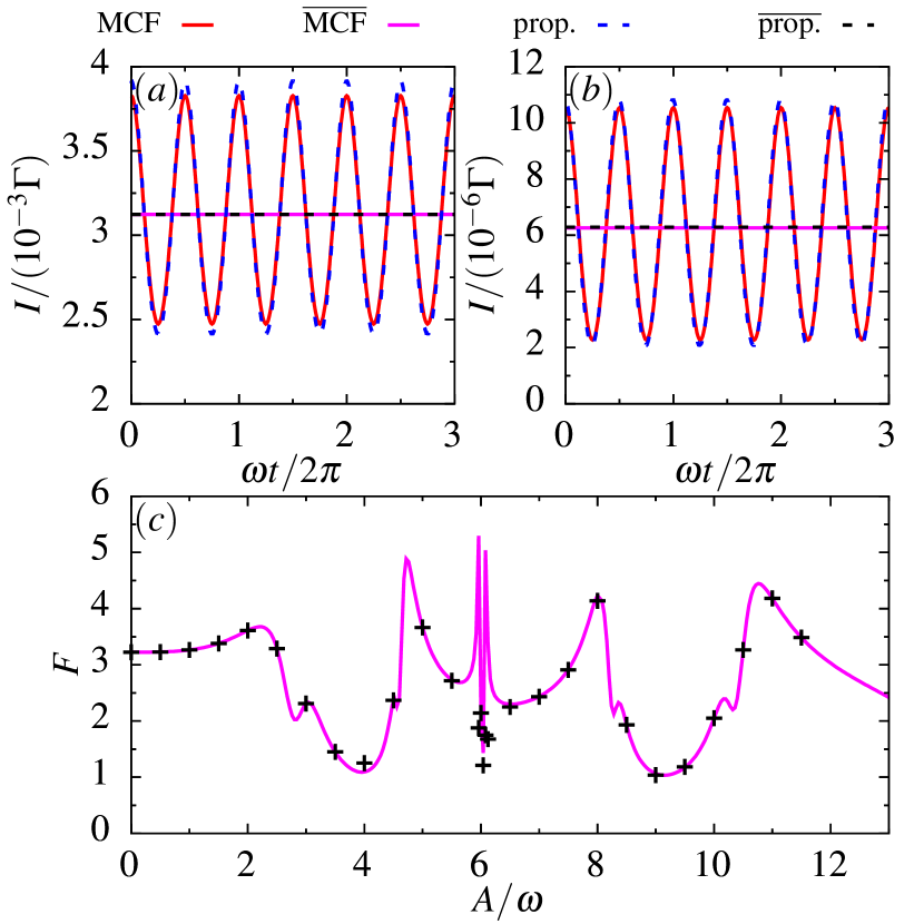
Figure 6: Time dependence of the current expectation value in the steady state for a chain with length $N=14$, (a) $\delta\tau=0.2\tau_{0}$, $b=0.4a$ and (b) $\delta\tau=-0.2\tau_{0}$, $b=0.6a$ obtained by means of propagation (prop.) and matrix-continued fractions (MCF). The respective average values are marked by horizontal lines. (c) Fano factor computed with matrix-continued fractions (solid line) compared to the result obtained by numerical propagation (dots) as a function of the amplitude of the driving for $\delta\tau=-0.2\tau_{0}$ and $b=0.6a$. The driving frequency is $\omega=5\tau_{0}$, while the chain-lead coupling reads $\Gamma=5\tau_{0}$.

The matrix-continued fraction method for the computation of the average current significantly reduces the computational effort as compared to the numerical propagation of the equations of motion (10) and (14), at least for large and intermediate driving frequencies and for parameters that lead to current blockade. To derive the former method, however, we had to assume that in Eq. (22), the time-dependent current $I(t)$ can be replaced by its time average Here we test this assumption and show in Figs. 6(a) and 6(b) the time-dependence of $I(t)$ in the steady-state limit. For typical driving parameters, we find that it possesses an appreciable ac component even though it is always smaller than the time average. In Fig. 6(c) we compare the results for the Fano factor computed with matrix-continued fractions and by numerical propagation. We find that, despite the neglected time-dependence, both results agree rather well. This justifies the approximation made in Sec. 2.3.

References

References

- [1] van der Wiel W G, De Franceschi S, Elzerman J M, Fujisawa T, Tarucha S and Kouwenhoven L P 2003 Rev. Mod. Phys. 75 1
- [2] Taubert D, Schuh D, Wegscheider W and Ludwig S 2011 Rev. Sci. Instrum. 82 123905
- [3] Elzerman J M, Hanson R, van Beveren L H W, Witkamp B, Vandersypen L M K and Kouwenhoven L P 2004 Nature (London) 430 431–435
- [4] Weinmann D, Häusler W and Kramer B 1995 Phys. Rev. Lett. 74 984
- [5] Weig E M, Blick R H, Brandes T, Kirschbaum J, Wegscheider W, Bichler M and Kotthaus J P 2004 Phys. Rev. Lett. 92 046804
- [6] Koch J and von Oppen F 2005 Phys. Rev. Lett. 94 206804
- [7] Hübener H and Brandes T 2009 Phys. Rev. B 80 155437
- [8] Benito M, Niklas M, Platero G and Kohler S 2016 Phys. Rev. B 93 115432
- [9] Grossmann F, Dittrich T, Jung P and Hänggi P 1991 Phys. Rev. Lett. 67 516
- [10] Großmann F and Hänggi P 1992 Europhys. Lett. 18 571
- [11] Holthaus M 1992 Phys. Rev. Lett. 69 351
- [12] Creffield C E and Platero G 2002 Phys. Rev. B 65 113304
- [13] Platero G and Aguado R 2004 Phys. Rep. 395 1
- [14] Kohler S, Lehmann J and Hänggi P 2005 Phys. Rep. 406 379
- [15] Stehlik J, Dovzhenko Y, Petta J R, Johansson J R, Nori F, Lu H and Gossard A C 2012 Phys. Rev. B 86 121303(R)
- [16] Forster F, Petersen G, Manus S, Hänggi P, Schuh D, Wegscheider W, Kohler S and Ludwig S 2014 Phys. Rev. Lett. 112 116803
- [17] Camalet S, Lehmann J, Kohler S and Hänggi P 2003 Phys. Rev. Lett. 90 210602
- [18] Gómez-León A and Platero G 2013 Phys. Rev. Lett. 110 200403
- [19] Dal Lago V, Atala M and Foa Torres L E F 2015 Phys. Rev. A 92 023624
- [20] Bello M, Creffield C E and Platero G 2016 Sci. Rep. 6 22562
- [21] Redfield A G 1957 IBM J. Res. Develop. 1 19
- [22] Blum K 1996 Density Matrix Theory and Applications 2nd ed (New York: Springer)
- [23] Breuer H P and Petruccione F 2003 Theory of open quantum systems (Oxford: Oxford University Press)
- [24] Forster F, Mühlbacher M, Blattmann R, Schuh D, Wegscheider W, Ludwig S and Kohler S 2015 Phys. Rev. B 92 245422
- [25] Su W P, Schrieffer J R and Heeger A J 1979 Phys. Rev. Lett. 42 1698
- [26] Asbóth J K, Tarasinski B and Delplace P 2014 Phys. Rev. B 90 125143
- [27] Bagrets D A and Nazarov Y V 2003 Phys. Rev. B 67 085316
- [28] Risken H 1989 The Fokker-Planck equation 2nd ed (Springer Series in Synergetics vol 18) (Berlin: Springer)
- [29] Platero G and Aguado R 1997 Appl. Phys. Lett. 70 3546
- [30] Zak J 1989 Phys. Rev. Lett. 62 2747
- [31] Delplace P, Ullmo D and Montambaux G 2011 Phys. Rev. B 84 195452
- [32] Lindner N H, Refael G and Galitski V 2011 Nature Phys. 7 490
- [33] Grushin A G, Gómez-León A and Neupert T 2014 Phys. Rev. Lett. 112 156801
- [34] Usaj G, Perez-Piskunow P M, Foa Torres L E F and Balseiro C A 2014 Phys. Rev. B 90 115423
- [35] Blanter Y M and Büttiker M 2000 Phys. Rep. 336 1
- [36] Emary C, Pöltl C, Carmele A, Kabuss J, Knorr A and Brandes T 2012 Phys. Rev. B 85 165417
- [37] Atala M, Aidelsburger M, Barreiro J T, Abanin D, Kitagawa T, Demler E and Bloch I 2013 Nature Physics 9 795