An explicit asymptotic preserving low Froude scheme for the multilayer shallow water model with density stratification

Abstract

We present an explicit scheme for a two-dimensional multilayer shallow water model with density stratification, for general meshes and collocated variables. The proposed strategy is based on a regularized model where the transport velocity in the advective fluxes is shifted proportionally to the pressure potential gradient. Using a similar strategy for the potential forces, we show the stability of the method in the sense of a discrete dissipation of the mechanical energy, in general multilayer and non-linear frames. These results are obtained at first-order in space and time and extended using a simple second-order MUSCL extension. With the objective of minimizing the diffusive losses in realistic contexts, sufficient conditions are exhibited on the regularizing terms to ensure the scheme’s linear stability at first and second-order in time and space. The other main result stands in the consistency with respect to the asymptotics reached at small and large time scales in low Froude regimes, which governs large-scale oceanic circulation. Additionally, robustness and well-balanced results for motionless steady states are also ensured. These stability properties tend to provide a very robust and efficient approach, easy to implement and particularly well suited for large-scale simulations. Some numerical experiments are proposed to highlight the scheme efficiency: an experiment of fast gravitational modes, a smooth surface wave propagation, an initial propagating surface water elevation jump considering a non trivial topography, and a last experiment of slow Rossby modes simulating the displacement of a baroclinic vortex subject to the Coriolis force.

1 Introduction

The study of geophysical phenomena involves three-dimensional and turbulent free surface flows with complex geometries. Numerical simulation of such flows still remains a very demanding challenge, continuously motivated by environmental, security or economic issues. Since the past decades, substantial advances have been realized in terms of mathematical modelling to reduce the original primitive equations complexity, leading to the emergence of shallow water models. In the particular case of oceans, the density stratification, which is mainly related to the temperature and salinity variations, can profoundly affect the water flow dynamics. Taking these aspects under consideration, the inviscid multilayer shallow water model, which involves an arbitrary number of superposed immiscible layers, offers a simple way to integrate the vertical density distribution with a satisfactory time computation request. The model presented in this work thus corresponds to a vertical discretization of the primitive equations, where the flow is described through a superposition of layers with constant density, as detailed in [56], and shown in Fig.1. One should note that, thanks to a general formulation of the pressure law, the model and associated numerical scheme presented in this work has a larger applicability range, possibly unrelated to large-scale oceanic circulation. Let us mention for instance the single-layer case, with specific one or two-dimensional applications to hydraulic or coastal engineering, or the Euler equations for gas dynamics.

Figure 1: Multilayer shallow water model with density stratification sketch. $h_{i},u_{i},\rho_{i}$ respectively stand for the water height, horizontal velocity field and density of the fluid in the i-th layer. $\eta_{i}=z_{b}+\sum_{k=i}^{{}^{L}}h_{k}$ is the water surface elevation with respect to the bottom topography $z_{b}$, and the effective mass in each layer is $H_{i}=h_{i}\rho_{i}$. All the model variables are collocated along the $z$ coordinate.

Naturally, allowing an arbitrary number of layers confers a much more complex nature to the flow. Indeed, in addition to non-linearities, it is a known fact that the multilayer equations exhibit particular structural properties, making the system theoretically and numerically more demanding. For instance, the hyperbolic structure can be violated if the shear velocity between two layers is too high, possibly leading to Kelvin-Helmholtz instabilities. Preventing the complex eigenvalues appearance is a quite complicated task, and this possible local hyberbolicity loss can significantly reduce the application range of the numerical schemes. These stability conditions are rigorously characterized in [40], where a general criterion of hyperbolicity and local well-posedness is given, under a particular asymptotic regime and weak stratification assumptions of the densities and the velocities. A similar study has been realized in [25] in the limit of small density contrast. It is shown that, under reasonable conditions on the flow, the system is well-posed on a large time interval. A second notable difficulty comes from the pressure law, introducing a non conservative coupling between the layers in the general case.

As a consequence, if a large range of approaches devoted to the single layer case are available in the literature, with the handling of complex geometries and rugged topography using unstructured environments ([12], [31], [42]), robust treatment of friction forces with wetting and drying ([17], [20], [41]), and allowing high order resolutions ([26], [60], [39]), the quantity of advances concerning the multilayer system is less plentiful. Nevertheless, when the number of layers is restricted to two, several techniques have been proposed on the basis of classical non-linear stability criteria, generally borrowed from the advances made on the single layer system. Thus, as concerns the two layers approximations, one can note for instance the Q-scheme proposed in [19], the recent relaxation approach [4] able to guarantee the preservation of motionless steady states, or the so called central-upwind scheme in [32]. Other splitting and upwind schemes can be found, with for instance in [18] (see also its extension to three layers proposed in [21] with a study of the hyperbolicity range), the f-wave propagation finite volume method in [38] handling dry states or the well-balancing and positivity-preserving results established in [10] within a splitting approach. At last, numerical methods for one-dimensional multilayer shallow water models with mass exchange are also proposed without density stratification in [6] and with in [5]. The approach is quite different since the layer depths are not independent variables and only the free surface is treated, and also because a part of the coupling terms are treated as a source term.

That being so, and although a first relevant approximation for ocean modelling may be provided by a bi-fluid stratification, the number of layers involved in most of current oceanic flow simulations with modern operational softwares is much more important in practice, in the order of several tens. This level of refinement ensures a reasonable compromise between the needs imposed by an accurate vertical discretization and computational constraints. Unfortunately, extending the approaches previously mentioned to the general case is quite difficult to achieve. One of the reasons is that they are not specially designed to preserve the asymptotics observed in low Froude number regimes. This requirement is mandatory for the simulation of oceanic flows, since the velocities magnitude are very moderate compared to the gravity wave speed far from the coast. Considering the integration time of realistic simulations, this limitation is also due to the paramount importance of the mechanical energy dissipation, which has to be guaranteed in order to produce physically acceptable solutions.

Adapting the choices made to express the distribution of the pressure law, which is also generally formulated, in some sense, by mean of staggered discretizations of the vertical direction, the multilayer equations formulated in this work are closely connected to those used in the majority of operational oceanic simulation softwares like HYCOM [11], ROMS [49] or NEMO [37], in isopycnal coordinates (i.e. when the flow is represented along the lines of constant density). These softwares have been developed on staggered grids, sharing an Arakawa C-grid type as a general basis with orthogonal curvilinear coordinates to take into account irregular lateral boundaries. This kind of horizontal space discretization prevents from well known spurious computational modes observed in low Froude number regimes. The barotropic and baroclinic modes are resolved with a time splitting technique allowing to use different time steps, as the barotropic wave speed is much higher than the larger baroclinic one, and this allows to save time computation. The barotropic continuity equation is often resolved with a FCT (Flux Corrected Transport) scheme and the momentum equations discretized with centered schemes of order two or four. As concerns time integration, Leapfrog-type schemes are usually employed, coupled with stabilization procedures using a Robert-Asselin filter in order to minimize the dissipation. A detailed report outlining the stability aspects related to oceanic modelling is available in [33]. If these approaches have been largely successfully applied, they can exhibit some weaknesses for some practical applications. The global stability of the numerical methods is not always guaranteed, threatened for instance by the occurrence of vanishing water heights or the difficulty to handle boundary conditions.

The permanent willingness to improve the quality and the versatility of numerical resolutions gave rise to an incresing interest for unstructured geometries during the past decade. The use of such environments may appear of major interest for many practical applications, and notably for oceanic circulation, for which geometrical flexibility allows to describe complex shaped shoreline coastlines and many different scales. Thus, an increasing number of projects are based on unstructured meshes, coping with numerical and implementation issues that have not yet been overcomed on these geometries. In this connection, a quite complete review of the most recent results oriented toward ocean modelling can be found in [23]. The SLIM [3] and FVCOM [2] projects can be cited as examples. Among the available works, mention can be made of [47] with the study of Finite Element methods stability applied to the rotating shallow water equations. It is concluded that all the numerical schemes considered are, at some point, concerned with spurious solutions. Some reference works devoted to the derivation of numerical schemes for the single layer rotating shallow water equations using unstructured meshes can be cited, as for instance the collocated upwind Finite Volume approach in [8], or the works on hexagonal staggered grids in [46] and [54], dedicated to the geostrophic balance and the modelling of Rossby waves. These works were recently extended in [22] in the context of higher order discretizations. Note that such stability problems were recently addressed on regular C-grids in [50], where the issue of mechanical energy conservation is also investigated. Note also the fully unstructured edge-based method available in [52], or the staggered scheme [28] devoted to the conservation of mechanical energy.

The present work describes a numerical strategy devoted to approximate the solutions of the two-dimensional multilayer shallow water system with a density stratification. The scheme is formulated in a fully explicit context and applicable for general meshes. On the basis of the constraints discussed above, the main objective is the enforcement of two essential stability results that are the asymptotic-preserving property with respect to low Froude number regimes, and the discrete dissipation of mechanical energy. The outline of this paper is organized as follows. In §2, we propose a regularization of the model that allows a better control of the mechanical energy production. We then give the formulation of the explicit scheme, designed to provide a discrete equivalent to this formalism, i.e. that allows the decrease of the mechanical energy. The §3 is devoted to stability issues. Well-balanced and robustness properties are addressed first. We then show a control on the mechanical energy production, and put it in correlation with our investigations in the linear case. Asymptotic preserving properties are established in a semi-continuous context in §4. A last step of numerical validation is finally proposed to assess the scheme abilities for large-scale simulations. Four test cases are proposed, implying the study of linear and non-linear solutions, analysis of convergence rate considering a non trivial topography, discontinuous solutions, and a last test in a realistic context.

2 Preliminaries

2.1 Physical model

Denoting $L$ the number of layers involved in the description of the flow, $t$ and $\mathbf{x}=(x,y)$ the time and space variables, the dynamics is governed by a general conservation law which consists of a set of $3\times L$ equations linking the mass in each layer $H_{i}(t,\mathbf{x})\geq 0$ to the horizontal velocity $\mathbf{u}_{i}(t,\mathbf{x})$. The system is submitted to gravitational forces through the scalar potential $\Phi_{i}({\boldsymbol{H}},\mathbf{x})$, where ${\boldsymbol{H}}=\,^{t}\left(H_{1},\cdots,H_{L}\right)$:

$$\left\{\begin{array}[]{lclcl}\partial_{t}H_{i}&+&\mathrm{div}\left(H_{i}{\textbf{u}_{i}}\right)&=&0\\ \partial_{t}(H_{i}{\textbf{u}_{i}})&+&\mathrm{div}\left(H_{i}{\textbf{u}_{i}}\otimes{\textbf{u}_{i}}\right)&=&-H_{i}\nabla\Phi_{i}/\varepsilon^{2}\end{array}\,.\right.$$ (1)

In the above equations, the parameter $\varepsilon$ is introduced to account for the scale factor between inertial and potential forces. This ratio is commonly referred to as Froude number or Mach number, depending on the physical context. Similarly, the scalar potential $\Phi_{i}$ introduced to account for the pressure law may take different formulations. In the case of the multilayer shallow water system, and assuming a constant density ${\rho_{i}}$ for each layer $i$, the effective mass corresponds to $H_{i}={\rho_{i}}{h_{i}}$, ${h_{i}}$, standing for the layer thickness (see Fig.1). Then, denoting by $z_{b}$ the bottom topography, the scalar potential is given by (see [56]) :

$${\Phi_{i}}=g\left(z_{b}+{\displaystyle{\sum_{j=1}^{L}}\dfrac{{\rho_{j}}}{\rho_{\max(i,j)}}{h_{j}}}\right)\,.$$ (2)

From a more general viewpoint, the potential and kinetic energies attached to the system are defined by $\partial_{H_{i}}\mathcal{E}={\Phi_{i}}$ and ${\mathcal{K}_{i}}=\dfrac{1}{2}H_{i}\left\|\textbf{u}_{i}\right\|^{2}$. We recall the conservation law satisfied by the mechanical energy $E=\mathcal{E}/\varepsilon^{2}+{\displaystyle{\sum_{i=1}^{L}}\>{\mathcal{K}_{i}}}$ for regular solutions, corresponding to the second law of thermodynamics:

$$\partial_{t}E+{\sum_{i=1}^{L}}\>\mathrm{div}\Big{(}\left(H_{i}{\Phi_{i}}/\varepsilon^{2}+{\mathcal{K}_{i}}\right)\,{\textbf{u}_{i}}\Big{)}=0\,.$$ (3)

As concerns numerical resolution of (1), based on the constraints discussed above, several guidelines are to be followed, principally based on two particular stability criteria. The first one, that has so far not been rigorously addressed in the general multilayer case, concerns the capability to describe the low Froude number asymptotics (i.e. when $\varepsilon\ll 1$). In these regimes, and as shown in our numerical experiments, Godunov-type schemes may bring too much dissipation and do not guarantee a good description of the flow. It is therefore crucial to work on the basis of rigorous consistency results. As stated in [24] in the context of Euler equations, these asymptotic behaviours are principally governed by the gradient pressure treatment (corresponding to $\nabla\Phi_{i}$ in (1)), for which centred approaches should be favoured.

The second essential point is related to the mechanical energy dissipation. More precisely, this means that the total energy attached to the discrete system will not increase in time, in accordance with the continuous frame (3). This property is crucial for geophysical flows, since an inappropriate discretization of the system may lead to energy production and break the stability of the system in large times. Such considerations of physically admissible solutions are studied in the numerical approach [15] for the one-dimensional model, where a semi-discrete entropy inequality is established in addition to the well-balancing property, treating the non-conservative coupling part as a source term. A stronger result is obtained in the two layers case with a fully discrete version [14]. An interesting approach can be found in [30], in the context of a compressible multifluid model. Inspired from the ideas of the AUSM methods for gas dynamics (see [36] and [35]) the formalism implies a modified velocity transport, shifted proportionally to the pressure gradient, whose goal is to provide a control on the energy budget at the continuous level. On this basis, a simple and efficient Finite Volume like scheme is derived, designed to provide a discrete equivalent of this result. More recently, a general extension has been proposed in [44] with the semi-implicit scheme for the two-dimensional multilayer shallow water model. Note that in addition, the mentioned approaches have the common feature of being asymptotic-preserving with respect to low Froude number regimes, notably thanks to a centred discretization of the pressure gradient, as discussed above.

To get a better picture of the formalism, we point out that this strategy can be interpreted at the continuous level as a discrete form of the following regularized model:

$$\left\{\begin{array}[]{lclcl}\partial_{t}H_{i}&+&\mathrm{div}\left(H_{i}\left(\textbf{u}_{i}-\delta\textbf{u}_{i}\right)\right)&=&0\\ \partial_{t}(H_{i}\textbf{u}_{i})&+&\mathrm{div}\left(H_{i}\textbf{u}_{i}\otimes\left(\textbf{u}_{i}-\delta\textbf{u}_{i}\right)\right)&=&-H_{i}\nabla\Phi_{i}/\varepsilon^{2}\end{array}\,,\right.$$ (4)

$\delta{\textbf{u}_{i}}$ standing for a generic perturbation on the velocity. This modification has the following impact on the energy conservation (3):

$$\partial_{t}E+\sum_{i=1}^{L}\>div\Big{(}\left(H_{i}\Phi_{i}/\varepsilon^{2}+\mathcal{K}_{i}\right)\,\left(\textbf{u}_{i}-\delta\textbf{u}_{i}\right)\Big{)}=-\sum_{i=1}^{L}\>\delta\textbf{u}_{i}.\nabla\Phi_{i}/\varepsilon^{2}\,,$$ (5)

which formally justifies a calibration of $\delta{\textbf{u}_{i}}$ in terms of the pressure gradient, to ensure a global decrease of the mechanical energy.

Following these lines, we aim at proposing a discrete equivalent of (5), in a fully explicit context. In this environment, the use of a shifted velocity transport $\left({\textbf{u}_{i}}-\delta{\textbf{u}_{i}}\right)$ is not sufficient to ensure a mechanical energy control, and a correction term is also needed on the scalar potential $\Phi_{i}$. It may also be shown that this adjustment, expressed in terms of discharge divergence, has also regularizing virtues on the energy budget at the continuous level. The practical advantages of an explicit formulation in comparison with the semi-implicit formulation proposed in [44] stand in the exemption of resolving the nonlinear system arising from for the continuity equation, an easier implementation of boundary conditions, and high order extensions in space and time can be more relatively easily derived. If the time step can be more restrictive, it is far from being obvious to compare the relative performances of the explicit and semi-implicit approaches in terms of accuracy vs. computation time. The particular difficulty to derive high order time stepping schemes for semi-implicit strategies without loosing strong stability properties makes things worse. At last, mixed formulations can also be derived decoupling the time advancement of the fast barotropic mode with the semi-implicit scheme, and the slow baroclinic modes using the explicit scheme, like it is already done in oceanic simulation softwares. Such a numerical model, that couples the benefits of the two approaches, is currently under study.

As mentioned before, the equations (1) enjoys a large range of applicability, so that the present approach is not only limited to large-scale oceanic circulation. Generally, we need the following regularity hypothesis on the potential forces:

Hypothesis 2.1.

Regularity assumptions on the potential forces

• The potential $\mathcal{E}$ is a regular and convex function of the mass, which means that the Hessian ${\boldsymbol{\mathcal{H}}}$ given by (see [56]):

  $${\boldsymbol{\mathcal{H}}_{ij}}=\partial_{H_{i}{H_{j}}}^{2}\mathcal{E}=\partial_{{H_{j}}}{\Phi_{i}}\>,\>(i,j)\in\llbracket 1,\ldots,L\rrbracket^{2}\>,\>$$ (6)

  is positive-definite.

• The potential is a symmetric and linear function of the mass, that is $\Phi={\boldsymbol{\mathcal{H}}}.\boldsymbol{H}$ and ${\boldsymbol{\mathcal{H}}}$ symmetric.

• The $L^{2}$ norm of ${\boldsymbol{\mathcal{H}}}$ is uniformly bounded with respect to space and time, more precisely:

  $$|||{\boldsymbol{\mathcal{H}}}(\boldsymbol{H},\mathbf{x})|||_{L^{2}}\,\leq\,{C_{{\boldsymbol{\mathcal{H}}}}}\,.$$ (7)

Remark 2.2.

In the case where the scalar potential is given by (2), the Hessian ${\boldsymbol{\mathcal{H}}}({\boldsymbol{H}},\mathbf{x})$ is constant in space and time:

$${\boldsymbol{\mathcal{H}}}_{i,j}=g\>\rho_{j}/\rho_{max(i,j)}\,,$$ (8)

and the requirements listed in Hypothesis 2.1 are trivially satisfied. The $L^{2}$ norm of $\mathcal{H}$ is thus evaluated in a pre-processing step, and we simply take ${C_{{\boldsymbol{\mathcal{H}}}}}\,=|||{\boldsymbol{\mathcal{H}}}(\boldsymbol{H},\mathbf{x})|||_{L^{2}}.$ Note also that this formulation automatically brings the conservation of the total momentum, as shown in [44]. However, this is not sufficient to guarantee the well-posedness of the problem: some conditions can be found in [40], regarding ${\boldsymbol{\mathcal{H}}}$ as a natural symmetrizer of the system. These conditions are based on smallness assumptions on the shear velocity and are sufficient to ensure that the system is hyperbolic. These low-shear conditions, easy to check numerically, were always widely satisfied in our operational situations. Hence, these aspects will not be discussed further in this work, and we refer to the references above for details.

2.2 Notations

We consider in this work a tesselation $\mathbb{T}$ of the computational domain $\Omega\subset\mathbb{R}^{2}$. We will denote ${m_{K}}$ the area and ${m_{\partial K}}$ the perimeter of a cell $K\in\mathbb{T}$. The boundary of $K$ will be denoted $\partial K$, and for any edge $e\in\partial K$, ${m_{e}}$ the length of the corresponding boundary interface and $\textbf{n}_{e,K}$ the outward normal to $e$ pointing to the neighbour $K_{e}$ (see Fig.2).

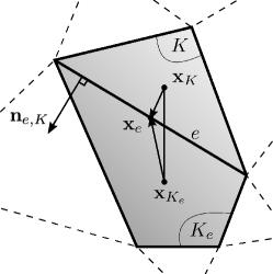
Figure 2: Geometric settings - Focus on the edge $e\in\partial K\cap\partial K_{e}$; $\textbf{n}_{e,K}$ is the outward normal to $e$, pointing to $K_{e}$, $\mathbf{x}_{K}$ indicates the mass center of $K$ and $\mathbf{x}_{e}$ is the middle of $e$.

Let’s now introduce some useful notations. For a scalar piecewise constant function $w$ we define:

$$\overline{w}_{e}=\dfrac{1}{2}\left(w_{K_{e}}+w_{K}\right)\quad,\quad\boldsymbol{\delta}w_{e}=\dfrac{1}{2}\left(w_{K_{e}}-w_{K}\right)\textbf{n}_{e,K}\,,$$

and similary, for a piecewise constant vectorial function w:

$$\overline{\textbf{w}}_{e}=\dfrac{1}{2}\left(\textbf{w}_{K_{e}}+\textbf{w}_{K}\right)\quad,\quad{\delta}\textbf{w}_{e}=\dfrac{1}{2}\left(\textbf{w}_{K_{e}}-\textbf{w}_{K}\right).\textbf{n}_{e,K}\,.$$

We also set: $w^{\pm}=\dfrac{1}{2}(w\pm|w|)$ the positive and negative parts of a scalar function $w$.

2.3 Numerical approach

The numerical scheme we consider is the following:

$$H_{K,i}^{n+1} \;=\; H_{K,i}^{n} \;-\; {\displaystyle\dfrac{\Delta t}{m_{K}}\sum_{e\in\partial K}\left(\mathcal{F}_{e,i}^{n}.\mathbf{n}_{e,K}\right)m_{e}}$$ (9a)

$$H_{K,i}^{n+1}\mathbf{u}_{K,i}^{n+1} \;=\; H_{K,i}^{n}\mathbf{u}_{K,i}^{n} \;-\; \dfrac{\Delta t}{m_{K}}\sum_{e\in\partial K}\left(\mathbf{u}_{K,i}^{n}\left(\mathcal{F}_{e,i}^{n}.\mathbf{n}_{e,K}\right)^{+}+\mathbf{u}_{K_{e},i}^{n}\left(\mathcal{F}_{e,i}^{n}.\mathbf{n}_{e,K_{e}}\right)^{-}\right)m_{e}$$ (9b)

$$\;-\; \dfrac{\Delta t}{m_{K}}H_{K,i}^{n}\sum_{e\in\partial K}\left(\dfrac{\Phi_{e,i}^{n,\ast}}{\varepsilon^{2}}\mathbf{n}_{e,K}\right)m_{e}$$

where we have set:

$$\mathcal{F}_{e,i}^{n} \;=\; \overline{H\textbf{u}}_{e,i}^{n}-\Pi_{e,i}^{n} \;=\; \left(\dfrac{H_{K,i}^{n}\textbf{u}_{K,i}^{n}+H_{K_{e},i}^{n}\textbf{u}_{K_{e},i}^{n}}{2}\right)-\Pi_{e,i}^{n}\,,$$ (10a)

$$\Phi_{e,i}^{n,\ast} \;=\; \overline{\Phi}_{e,i}^{n}-\Lambda_{e,i}^{n} \;=\; \left(\dfrac{\Phi_{K,i}^{n}+\Phi_{K_{e},i}^{n}}{2}\right)-\Lambda_{e,i}^{n}\,.$$ (10b)

The quantities ${\Lambda_{e,i}^{n}}$ and $\Pi_{e,i}^{n}$ introduced above stand for the perturbations respectively assigned to the potential forces and numerical fluxes, designed to ensure the stability of the method. They are defined as follows:

$$\Pi_{e,i}^{n} =\gamma\>\Delta t\>\left(\frac{\widehat{H}}{\text{$\Delta$}}\right)_{e,i}^{n}\>\dfrac{\boldsymbol{\delta}\Phi_{e,i}^{n}}{\varepsilon^{2}}\quad,\quad\gamma\geq 0\,,$$ (11)

$$\Lambda_{e,i}^{n} ={\normalcolor{\normalcolor{\color[rgb]{0,.5,.5}{\normalcolor\alpha\>\Delta t\>\left(\frac{C_{\boldsymbol{\mathcal{H}}}}{\Delta_{e}}\right)\>\delta(H\textbf{u})_{e,i}^{n}}}}}\quad,\quad\alpha\geq 0\,,$$ (12)

with the geometric constant:

$$\frac{1}{\Delta_{e}}=\dfrac{1}{2}\left(\frac{1}{\Delta_{K}}+\frac{1}{\Delta_{K_{e}}}\right)=\dfrac{1}{2}\left(\dfrac{m_{\partial K}}{m_{K}}+\dfrac{m_{\partial K_{e}}}{m_{K_{e}}}\right)\,,$$ (13)

where $d$ is the problem dimension, and the weighted average:

$$\left(\frac{\widehat{H}}{\text{$\Delta$}}\right)_{e,i}^{n}=\dfrac{1}{2}\left(\left(\frac{\widehat{H}}{\text{$\Delta$}}\right)_{K,i}^{n}+\left(\frac{\widehat{H}}{\text{$\Delta$}}\right)_{K_{e},i}^{n}\right)=\dfrac{1}{2}\left(\widehat{H}_{K}^{n}\dfrac{m_{\partial K}}{2m_{K}}+\widehat{H}_{K_{e}}^{n}\dfrac{m_{\partial K_{e}}}{2m_{K_{e}}}\right)\,,$$ (14)

where $\widehat{H}_{K}^{n}$ is $H_{K}^{n}$ in practice and for all the presented simulations. Nervertheless, for simplification purposes, the non-linear stability analysis developed in this work implies an implicit definition of $\widehat{H}_{K}^{n}$, according to (72) (see Remark 2.4 below). We also refer to Theorem 3.4 and subsequent Remark 3.6 for the calibration of the stabilization constants $\alpha$ and $\gamma$.

As the increase of space and time order will be discussed throughout the paper, we give the second-order extensions in space and time in the Appendix 7.3. A MUSCL spatial reconstruction scheme (7.3.2) is used (substituting at each side of the edge $e$ the primitive variables $H_{K}$, $\mathbf{u}_{K}$, $H_{K_{e}}$ and $\mathbf{u}_{K_{e}}$ by reconstructed primitive variables $H_{e,K}$, $\mathbf{u}_{e,K}$, $H_{e,K_{e}}$ and $\mathbf{u}_{e,K_{e}}$ to evalutate the numerical fluxes in (9a) and (9b)). The temporal discretization is achieved using the Heun’s method (7.4).

Remark 2.3.

$\Pi_{e,i}^{n}$ is related to the potential pressure gradient $\boldsymbol{\delta}\Phi_{e,i}^{n}$ and is intended to reproduce the stabilizing effects of the generic perturbation $\delta\textbf{u}_{i}$ introduced in the continuous frame in (4) to regularize the energy budget (5). Similarly, it can be shown that the continuous equivalent of $\Lambda_{e,i}^{n}$, which involves an approximation of the discharge divergence, brings an additional dissipation term in (5).

Remark 2.4.

$\widehat{H}_{K,i}^{n}$ is indeed explicit in practice. If the mechanical energy dissipation will be demonstrated here with an implicit definition of $\widehat{H}_{K,i}^{n}$ according to (72), taking $\widehat{H}_{K}^{n}=H_{K,i}^{n}$ introduces an error in $\mathcal{O}(\Delta t)$ and is widely sufficient to preserve the overall stability. These conclusions have been reached with the support of many numerical experiments (including the propagation of discontinuous initial solutions), with a particular focus on low Froude number regimes ($\varepsilon\ll 1$), for which we observed no significant impact. Moreover, the proof of mechanical energy dissipation proposed in Appendix 7.1 can be realized in a fully explicit way, at the price of a more complex analysis and a slight adaptation of $\Pi_{e,i}^{n}$, leading to very similar results. For readability reasons we chose not to detail this proof and some insights are available in Remark 3.7. The implicit definition of $\widehat{H}_{K,i}^{n}$ in the non-linear stability proof is considerably lighter and provides a good overview of the employed strategy.

Let us finally remark that the numerical scheme satisfied by the velocity is:

$$\textbf{u}_{K,i}^{n+1}=\textbf{u}_{K,i}^{n}-\dfrac{\Delta t}{m_{K}}{\sum_{e\in\partial K}}\dfrac{{\textbf{u}_{K_{e},i}^{n}}-\textbf{u}_{K,i}^{n}}{{H_{K,i}^{n+1}}}{\big{(}\mathcal{F}_{e,i}^{n}.\textbf{n}_{e,K}\big{)}^{-}}{m_{e}}-\dfrac{\Delta t}{m_{K}}\dfrac{{H_{K,i}^{n}}}{{H_{K,i}^{n+1}}}{\sum_{e\in\partial K}}\dfrac{{\Phi_{e,i}^{n,\ast}}}{\varepsilon^{2}}\textbf{n}_{e,K}{m_{e}}\,,$$ (15)

and note that:

$${\sum_{e\in\partial K}}{\Phi_{e,i}^{n,\ast}}\textbf{n}_{e,K}{m_{e}}={\sum_{e\in\partial K}}{\boldsymbol{\delta}\Phi_{e,i}^{n}}{m_{e}}-{\sum_{e\in\partial K}}{\Lambda_{e,i}^{n}}\textbf{n}_{e,K}{m_{e}}\,,$$ (16)

since the main term of (10b) involves a centred discretization of the potential.

We finally recall the explicit CFL condition on which are usually based Godunov-type schemes (see [29]):

$$\left(|\overline{\textbf{u}}_{e,i}^{n}.\textbf{n}_{e,K}|+\dfrac{c_{e,i}^{n}}{\varepsilon}\right)\Delta t\max\left(\dfrac{{m_{e}}}{{m_{K}}},\dfrac{{m_{e}}}{{m_{K_{e}}}}\,\right)\leq\tau_{CFL}\,,$$ (17)

where $\left(c_{e,i}^{n}\right)_{1\leq i\leq L}$ corresponds to the square root of the eigenvalues of the matrix $H_{i}{\boldsymbol{\mathcal{H}}}_{i,j}$.

3 Stability issues

In this section we focus on crucial linear and non-linear stability criterion: motionless steady states preservation, water height positivity preservation, mechanical energy dissipation and linear stabily analysis. These essential points need to be integrated in the construction of numerical schemes expected to respond to practical issues. Traditionally, providing a numerical approach able to account for all these aspects simultaneously remains a quite complicated task, especially in the context of general geometries and stratified multiscale models. Nevertheless, the formalism employed here allows a quite simple treatment of well-balanced and robustness properties. We finally provide the complete linear stability analysis in order to derive relaxed stability conditions comparatively to ones ensuring the mechanical energy dissipation which are not optimal. Indeed, it will be shown that the linear stability conditions are far less restrictive.

3.1 Well Balancing

As a first stability criterion we study the problem of steady states preservation. From a general point of view, regarding the difficulty to derive and handle numerically the full set of steady states observed in most of realistic evolution processes, it is classical to focus first on rest states. In our formalism, this leads to the following trivial solution:

$$\textbf{u}_{K,i}=0\quad,\quad\Phi_{K,i}=\Phi_{i}\,,$$

for all volume control $K$ and layer $i$. This trivial solution is nothing but the generalization to the multilayer case of the classical lake at rest solution in the $L=1$ case:

$$\textbf{u}=0\quad,\quad h+z_{b}=0\,,$$

which has indeed to be exactly preserved to avoid the appearance of non physical perturbations in the vicinity of flat free surface configurations. The capability to preserve these particular steady states already stands for a discriminating property, even in the one layer case, notably with the increasing interest of unstructured meshes and high order space schemes. In spite of these difficulties, the proposed discretization allows their exact preservation without needing any correction at first-order in space and in a very simple way at second-order. The following approach is thus intrinsically adapted to the preservation of such equilibria, standing for a good alternative to the classical well-balanced methods.

Proposition 3.1.

Well Balancing
The scheme (9a,9b) equipped with the numerical fluxes (10a) and discrete potential (10b) preserves the steady states at rest defined by $\textbf{u}_{K,i}^{n}=0$ and ${\Phi_{K,i}^{n}}=\Phi_{i}$.

Proof.

Since the perturbation $\Pi_{e,i}^{n}$ (12) is expressed in terms of ${\boldsymbol{\delta}\Phi_{e,i}^{n}}$, we immediately have $\mathcal{F}_{e,i}^{n}=0$ and (9a) gives ${H_{K,i}^{n+1}}={H_{K,i}^{n}}$. Then, since ${\Lambda_{e,i}^{n}}=0$, the momentum equation (9b) reduces to:

$${H_{K,i}^{n+1}}\textbf{u}_{K,i}^{n+1}=-\dfrac{\Delta t}{m_{K}}{H_{K,i}^{n}}\left(\dfrac{\Phi_{i}}{\varepsilon^{2}}\right)\left({\sum_{e\in\partial K}}\textbf{n}_{e,K}{m_{e}}\right)=0\,,$$ (18)

which allows to conclude.∎

The second-order MUSCL spatial reconstruction requires to evaluate a vectorial slope in each volume control K for all primitive variables (one can also compute the vectorial slopes from conservative or entropic variables to reconstruct at the end the primitive variables at the edge). The resulting scheme (83-84) produces a non well-balanced scheme in most of practical cases. This is because the water surface elevation ${\normalcolor\eta_{i}={\color[rgb]{0,.5,.5}{\normalcolor z_{b}+}}\sum_{k=i}^{{}^{L}}h_{k}}$ must be locally linear to produce for each edge $e$ two equal reconstructed water surface elevation $\eta_{K,i}$ and $\eta_{K_{e},i}$. As a consequence, the MUSCL spatial reconstruction breaks the well-balanced property demonstrated previously. One simple way to resolve this drawback is to evalute the vectorial slope for the water surface elevation $\eta_{i}$ rather than for the water height $h_{i}$. Considering an arbiratrary bed elevation $z_{b_{e}}$ at the edge $e$ (that can be directly evaluated from a continuous function or taking the half sum from the two adjacent volume control $K$ and $K_{e}$), the two water heights are finally evaluated substracting the edge bed elevation $z_{b_{e}}$ to the two reconstructed water surface elevation $\eta_{K,i}$ and $\eta_{K_{e},i}$.

3.2 Robustness

We investigate here the problem of robustness by proposing a CFL condition allowing to obtain the preservation of the water height positivity.

Proposition 3.2.

Robustness
We consider the numerical scheme (9a,9b) equipped with the numerical fluxes (10a) and discrete potential (10b). Assume a CFL condition of the type:

$$\Delta t\max\left(\dfrac{{m_{\partial K}}}{{m_{K}}},\dfrac{{m_{\partial K_{e}}}}{{m_{K_{e}}}}\right)\left(|\overline{\textbf{u}}_{e,i}^{n}.\textbf{n}_{e,K}|+\sqrt{\gamma}\sqrt{\dfrac{|{\boldsymbol{\delta}\Phi_{e,i}^{n}}|}{\varepsilon^{2}}}\right)\leq\left(\dfrac{\beta}{\beta+1}\right)\xi_{e,i}^{n}$$ (19)

for each edge $e=\partial K\cap\partial K_{e}$ , where $0<\beta\leq 1$ and:

$$\xi_{e,i}^{n}=\dfrac{\min\left({H_{K,i}^{n}},{H_{K_{e},i}^{n}}\right)}{\max\left({\widehat{H}_{K,i}^{n}},{\widehat{H}_{K_{e},i}^{n}},{H_{K,i}^{n}},{H_{K_{e},i}^{n}}\right)}\,.$$ (20)

Then:

$${H_{K,i}^{n+1}}\geq\dfrac{1}{\beta}\dfrac{\Delta t}{m_{K}}{\sum_{e\in\partial K}}-{\big{(}\mathcal{F}_{e,i}^{n}.\textbf{n}_{e,K}\big{)}^{-}}{m_{e}}\geq 0\,.$$ (21)

Proof.

The result being specific to each layer, we drop the subscript “i” for the sake of clarity. Gathering

$$\dfrac{\Delta t}{m_{K}}{\sum_{e\in\partial K}}-{\big{(}\mathcal{F}_{e}^{n}.\textbf{n}_{e,K}\big{)}^{-}}{m_{e}}\leq\dfrac{\Delta t}{m_{K}}{\sum_{e\in\partial K}}|\mathcal{F}_{e}^{n}.\textbf{n}_{e,K}|{m_{e}}\,,$$

and

$${H_{K}^{n+1}}\geq{H_{K}^{n}}-\dfrac{\Delta t}{m_{K}}{\sum_{e\in\partial K}}|\mathcal{F}_{e}^{n}.\textbf{n}_{e,K}|{m_{e}}\,,$$

we get:

$$\begin{split}\beta{H_{K}^{n+1}}-\dfrac{\Delta t}{m_{K}}{\sum_{e\in\partial K}}-{\big{(}\mathcal{F}_{e}^{n}.\textbf{n}_{e,K}\big{)}^{-}}{m_{e}}\geq\beta{H_{K}^{n}}&-(1+\beta)\dfrac{\Delta t}{m_{K}}{\sum_{e\in\partial K}}|{\overline{H\textbf{u}}_{e}^{n}}.\textbf{n}_{e,K}|{m_{e}}\\ &-(1+\beta)\dfrac{\Delta t}{m_{K}}\gamma\Delta t{\sum_{e\in\partial K}}\left(\frac{\widehat{H}}{\text{$\Delta$}}\right)_{e}^{n}\dfrac{|{\boldsymbol{\delta}\Phi_{e}^{n}}.\textbf{n}_{e,K}|}{\varepsilon^{2}}{m_{e}}\,.\end{split}$$

From this, a sufficient condition to obtain (21) can be expressed locally as:

$$\begin{split}&(1+\beta)\dfrac{\Delta t}{m_{K}}|{\overline{H\textbf{u}}_{e}^{n}}.\textbf{n}_{e,K}|+(1+\beta)\gamma\Delta t\dfrac{\Delta t}{m_{K}}\left(\frac{\widehat{H}}{\text{$\Delta$}}\right)_{e}^{n}\dfrac{|{\boldsymbol{\delta}\Phi_{e}^{n}}.\textbf{n}_{e,K}|}{\varepsilon^{2}}\,\leq\beta\dfrac{{H_{K}^{n}}}{{m_{\partial K}}}\,,\end{split}$$

This leads to:

$$\mu|\overline{\textbf{u}}_{e}^{n}.\textbf{n}_{e,K}|+\mu^{2}\gamma\dfrac{|{\boldsymbol{\delta}\Phi_{e}^{n}}.\textbf{n}_{e,K}|}{\varepsilon^{2}}\leq\left(\dfrac{\beta}{1+\beta}\right)\xi_{e}^{n}\,,$$ (22)

where $\mu=\Delta t\max\left(\dfrac{{m_{\partial K}}}{{m_{K}}},\dfrac{{m_{\partial K_{e}}}}{{m_{K_{e}}}}\right)$. Since the right member of the previous inequality is lower than $1$, we conclude that (22) is ensured under (19).

∎

Remark 3.3.

$\boldsymbol{\delta}\Phi_{e,i}^{n}$ being in the order of the mesh size, the advective terms govern the CFL condition (19), which is thus far less restrictive than a time step restriction of the form (17) in the case of practical applications implying low Froude numbers. Note also that in these contexts the water heights are far from zero, preventing the quantity $\xi_{e,i}^{n}$ (20) from being arbitrarily small. In practice, $\xi_{e,i}^{n}$ reduces to $\dfrac{\min\left({H_{K,i}^{n}},{H_{K_{e},i}^{n}}\right)}{\max\left({H_{K,i}^{n}},{H_{K_{e},i}^{n}}\right)}$ (see Remark 2.4) and is very nearly $1$. In more general terms, solutions are proposed in [12],[13] to deal with wet/dry fronts when considering CFL conditions of the form (19). From now, taking these aspects under consideration, we assume that for all $\beta>0$ the positivity result (21) holds under the CFL constraint (17). In other terms:

$$\dfrac{\Delta t}{m_{K}}{\sum_{e\in\partial K}}-{\big{(}\mathcal{F}_{e,i}^{n}.\textbf{n}_{e,K}\big{)}^{-}}{m_{e}}\leq\beta{H_{K,i}^{n+1}}\,.$$ (23)

In our stability results, we need $\beta=1/4$ (see (65) and below). We numerically verified that this time step restriction was always less restrictive than the classical explicit CFL condition given in (17), based on the gravity wave speed. Note, however, that $\beta$ can be taken smaller to obtain relaxed conditions on the stabilization constants $\alpha$ and $\gamma$ (see Remark 3.6).

3.3 Energy dissipation

The main result of the current section concerns the dissipation of the mechanical energy at the discrete level. Denoting ${E^{n}}={\displaystyle\sum_{K\in\mathbb{T}}{m_{K}}\left({\mathcal{E}_{K}^{n}}/\varepsilon^{2}+{\displaystyle{\sum_{i=1}^{L}}{\mathcal{K}_{K,i}^{n}}}\right)}$ the discrete energy at time $n$, we have the following result:

Theorem 3.4.

Control of the mechanical energy

We consider the numerical scheme (9a,9b), together with the corrected potential (10b,12):

$${\Phi_{e,i}^{n,\ast}}={\overline{\Phi}_{e,i}^{n}}-{\Lambda_{e,i}^{n}}\quad,\quad{\Lambda_{e,i}^{n}}=\alpha\Delta t{C_{{\boldsymbol{\mathcal{H}}}}}\frac{{{\delta}(H\textbf{u})_{e,i}^{n}}}{\Delta_{e}}\,\,,$$

and numerical fluxes (10a,11):

$$\mathcal{F}_{e,i}^{n}={\overline{H\textbf{u}}_{e,i}^{n}}-\Pi_{e,i}^{n}\quad,\quad\Pi_{e,i}^{n}=\gamma\Delta t\left(\frac{\widehat{H}}{\text{$\Delta$}}\right)_{e,i}^{n}\dfrac{{\boldsymbol{\delta}\Phi_{e,i}^{n}}}{\varepsilon^{2}}\,\,,$$

Assume that the time step is governed by an explicit CFL condition (17). Then, the stabilization constants

$$\gamma=4\;,\;\alpha=2$$

ensure the control of the mechanical energy production:

$${E^{n+1}}-{E^{n}}\leq\,0\,.$$ (24)

To establish the announced result, we first give an estimate for the kinetic and potential energy productions, and finally show that the choice $\gamma=4$ and $\alpha=2$ in (12) and (11) allows a global control of these contributions. The proof is given in Appendix 7.1 and organized around the following steps:

• $\#A$ - Estimation of the kinetic energy production (Appendix 7.1.1, Proposition 7.1).

• $\#B$ - Estimation of the potential energy production (Appendix 7.1.2, Proposition 7.2).

• $\#C$ - Control of the mechanical energy (Appendix 7.1.3): we gather the two inequalities resulting from $\#A$ and $\#B$ to deduce a sufficient condition on the stabilization constants $\gamma$ and $\alpha$ present in the correction terms (12, 11) .

Remark 3.5.

The proof is mainly based on the negativity of the quadratic polynomials given in (75) and (77), which dominant coefficient is expressed in terms of the following quantity:

$$\rho_{\varepsilon}^{2}=2\dfrac{\left(\Delta t\right)^{2}}{\varepsilon^{2}}\frac{C_{\boldsymbol{\mathcal{H}}}}{\Delta_{e}}\left(\frac{\widehat{H}}{\text{$\Delta$}}\right)_{e,i}^{n}\,.$$

A basic analysis of the discriminant gives admissibiliy conditions on $\rho_{\varepsilon}$ that are expected to limit the time step. In one dimension and in the single layer case for instance, the quantity $\rho_{\varepsilon}$ reduces to $2{\displaystyle\dfrac{\Delta t}{\Delta x}\dfrac{c}{\varepsilon}}$, where $c=\sqrt{gh}$ is the gravity wave speed, so that the smallness assumptions made on $\rho_{\varepsilon}$ are satisfied under a classical explicit CFL condition (i.e. of the form (17)). This is also the case for the general $L$ layers case in two dimensions, where the conditions required on $\rho_{\varepsilon}$ are always satisfied with such a time constraint.

Remark 3.6.

As it has been confirmed by our numerical experiments, if the values $\gamma=4$ and $\alpha=2$ ensure a global decrease of the mechanical energy, they also bring too much diffusion in practice, entailing dramatic restrictions on the space step. This compels us to seek for relaxed conditions, that can be extracted from a more general (and complex) analysis of the discrete energy budgets, not described here for the sake of readability. As a matter of fact, the optimality of the current approach has been lost within the Jensen’s inequalities used during the estimations of the kinetic and potential energies (formulas (64) and (71) respectively). If an explicit choice has been made on the weights to make things more concrete, a global result can be established introducing a general set of constants in these two inequalities. Playing with these parameters and $\beta$ (see CFL condition (19)), one can significantly relax the conditions on the stabilization constants. In the single layer case and one-dimensional problem for instance, the condition on $\gamma$ becomes:

$$\gamma\in\left[\gamma^{-},\gamma^{+}\right]\quad,\quad\text{with}\quad\gamma^{\pm}=\dfrac{1\pm\sqrt{1-\rho_{\varepsilon}^{2}}}{\rho_{\varepsilon}^{2}}\,,$$ (25)

where we recall that $\rho_{\varepsilon}=2\dfrac{\Delta t}{\Delta x}\dfrac{c}{\varepsilon}$. A very close result is obtained for $\alpha$:

$$\alpha\in\left[\alpha^{-},\alpha^{+}\right]\quad,\quad\text{with}\quad\alpha^{\pm}=\dfrac{1\pm\sqrt{1-2\rho_{\varepsilon}^{2}}}{2\rho_{\varepsilon}^{2}}\,.$$ (26)

When $\rho_{\varepsilon}$ (or equivalently the CFL number) decreases, a more important latitude regarding the choice of $\gamma$ and $\alpha$ is obtained, as illustrated in Fig.3. And when $\rho_{\varepsilon}$ tends to zero, one recovers the critical value $\gamma=\alpha=1/2$.

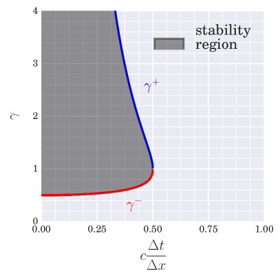
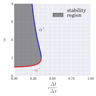
Figure 3: Non-linear discrete analysis: evolution of the lower and upper bounds for $\gamma$ (left) and $\alpha$ (right) with respect to the CFL number, based respectively on (25) and (26).

As a result, one can get stability taking $\alpha$ and $\gamma$ in the vicinity of $1/2$ at first-order in space and time, even in the general case of arbitrary stratifications. As it will be discussed later, less restrictive conditions will be extracted from the linear stability analysis (see §3.4) with the use of MUSCL space scheme (Appendix 7.3.2) coupled with the Heun’s method for time discretization (Appendix 7.4). Indeed, the stabilizing effects of the second-order time scheme allow to considerably relax the stabilization constants, in conformity with our numerical observations.

Remark 3.7.

As discussed in Remark 2.4, the rigorous definition of $\widehat{H}_{K}^{n}$ appearing in the numerical fluxes through (11,14) given in (72) implies an implicit time step. With the support of some numerical experiments, we already motivated the reasons of substituting $H_{K}^{n}$ to $\widehat{H}_{K}^{n}$ for practical applications, since this simplified choice only introduces an error in the order of $\Delta t$ and does not change the asymptotic behaviour of the scheme. However, we have to specify here that at the price of being slightly more restrictive, a fully explicit stability condition can be given. The strategy implies a global calibration of the stabilization parameters, (i.e. for which we set $\widehat{H}_{K,i}^{n}=\widehat{H}_{i}^{n}\thinspace,\thinspace\forall\thinspace K\in\mathbb{T}$), allowing to reduce to the study of a cubic polynomial (rather than quadratic) at the level of each element. For the sake of readability and to alleviate the proofs, we made the choice of presenting the scheme in its present form.

Remark 3.8.

As it has been discussed above, the negativity domain of the polynomials $p$ and $q$ defined in (75) and (77) respectively can be enlarged by diminishing the CFL. One of the consequences is that the control (24) can be extended to obtain a strict mechanical energy decrease. More precisely, let us consider a small parameter $\delta>0$, and a combination of values $\left(\Delta t,\alpha,\gamma\right)$ satisfying (75) and (77). Considering the dominant coefficient of $p$ and $q$, one easily obtains $p(\gamma)<-\delta$ and $q(\alpha)<-\delta$ with a time step $\Delta t$ subject to an $\mathcal{O}(\delta)$ perturbation. Then, gathering (73) and (76), we obtain:

$$\begin{split}{E^{n+1}}-{E^{n}}\leq\,&-\delta\left(\Delta t\right)^{2}\sum_{K}{\sum_{i=1}^{L}}{\sum_{e\in\partial K}}\left(\frac{\widehat{H}}{\text{$\Delta$}}\right)_{e,i}^{n}\left\|\dfrac{{\boldsymbol{\delta}\Phi_{e,i}^{n}}}{\varepsilon^{2}}\right\|^{2}{m_{e}}\,\\ &-\delta\left(\Delta t\right)^{2}\sum_{K}{\sum_{i=1}^{L}}{\sum_{e\in\partial K}}{C_{{\boldsymbol{\mathcal{H}}}}}\frac{1}{\Delta_{e}}\left(\dfrac{{{\delta}(H\textbf{u})_{e,i}^{n}}}{\varepsilon}\right)^{2}{m_{e}}\,.\end{split}$$ (27)

These estimates give a control of $L^{1}(0,T,H_{w}^{1}(\Omega))(u)$ with some ad hoc weighted semi-norm on $H_{w}^{1}$. They insure validity of Lax Wendroff type theorem for weak consistency of conservative terms (in divergence form) in mass, momentum and energy equations. We refer to [27] and also [59] for further details concerning the use of such estimates to study consistency and convergence of the methods.

3.4 Linear stability analysis

We aim here at assessing the relevance of the previous energy dissipation considerations through linear stability arguments. For the sake of clarity the developments of the current section are given for the one-dimensional problem, considering a regular mesh and the one layer case ($L=1$). We specify at the end how these results can be easily extended to the two-dimensional problem. The elements will be indexed by $k$ and we denote $\mathcal{F}_{k+1/2}^{n}$ the numerical edge flux between the cells $k$ and $k+1$. Let us take the example of negative fluxes, for which we have:

$$\begin{array}[]{l}\left(\mathcal{F}_{k+1/2}^{n}\right)^{-}=\mathcal{F}_{k+1/2}^{n}\quad\text{and}\quad\left(\mathcal{F}_{k+1/2}^{n}\right)^{+}=0\,.\end{array}$$

In that context the equations (9a), (15) constituting the first-order scheme simplify as follows:

$$\begin{split}&H_{k}^{n+1}=H_{k}^{n}-\dfrac{\Delta t}{\Delta x}\left(\mathcal{F}_{k+1/2}^{n}-\mathcal{F}_{k-1/2}^{n}\right)\,,\\ &u_{k}^{n+1}=u_{k}^{n}-\dfrac{\Delta t}{\Delta x}\left(\dfrac{u_{k+1}^{n}-u_{k}^{n}}{H_{k}^{n}}\mathcal{F}_{k+1/2}^{n}\right)-\dfrac{\Delta t}{\Delta x}{\color[rgb]{0,.5,.5}{\normalcolor\dfrac{H_{K,i}^{n}}{H_{K,i}^{n+1}}}}\left(\Phi_{k+1/2}^{n,\ast}-\Phi_{k-1/2}^{n,\ast}\right)\,.\end{split}$$ (28)

with the following numerical mass flux:

$$\mathcal{F}_{k+1/2}^{n}=\dfrac{H_{k}^{n}u_{k}^{n}+H_{k+1}^{n}u_{k+1}^{n}}{2}-2\gamma\dfrac{\Delta t}{\Delta x}\left(\dfrac{H_{k}^{n}+H_{k+1}^{n}}{2}\right)\left(\dfrac{\Phi_{k+1}^{n}-\Phi_{k}^{n}}{2}\right)\,,$$ (29)

and a corrected potential of the form:

$$\Phi_{k+1/2}^{n,\ast}=\left(\dfrac{\Phi_{k+1}^{n}+\Phi_{k}^{n}}{2}\right)-2\alpha\dfrac{\Delta t}{\Delta x}C_{\boldsymbol{\mathcal{H}}}\left(\dfrac{H_{k+1}^{n}u_{k+1}^{n}-H_{k}^{n}u_{k}^{n}}{2}\right)\,.$$ (30)

The scheme (28) is linearized around the constant state $\bar{w}=\left(\bar{H},\bar{u}\right)$. Introducing a generic perturbation $\tilde{w}_{k}^{n}=\left(\tilde{H}_{k}^{n},\tilde{u}_{k}^{n}\right)$ on the flow, we write:

$$H_{k}^{n}=\bar{H}+\tilde{H}_{k}^{n}\quad u_{k}^{n}=\bar{u}+\tilde{u}_{k}^{n}\,,$$

to obtain the following linearized system:

$${\tilde{H}_{k}^{n+1}} ={\tilde{H}_{k}^{n}}-\dfrac{\Delta t}{\Delta x}\left[\bar{H}\delta^{n}[\tilde{u}_{k}]+\bar{u}\delta^{n}[\tilde{H}_{k}]-2\gamma\bar{\Phi}_{H}\dfrac{\Delta t}{\Delta x}\bar{H}\Delta^{n}[\tilde{H}_{k}]\right]\,,$$ (31a)

$${\tilde{u}_{k}^{n+1}} ={\tilde{u}_{k}^{n}}-\dfrac{\Delta t}{\Delta x}\left[\bar{\Phi}_{H}\delta^{n}[\tilde{H}_{k}]+\bar{u}d_{+}^{n}[{\tilde{u}_{k}^{n}}]-2\alpha{C_{{\boldsymbol{\mathcal{H}}}}}\dfrac{\Delta t}{\Delta x}\left(\bar{H}\Delta^{n}[\tilde{u}_{k}]+\bar{u}\Delta^{n}[\tilde{H}_{k}]\right)\right]\,$$ (31b)

where we have set $\bar{\Phi}_{H}=\partial_{H}\Phi_{|\bar{H}}$, and with the following discrete operators:

$$\delta^{n}[f]=\dfrac{f_{k+1}^{n}-f_{k-1}^{n}}{2}\quad,\quad\Delta^{n}[f]=\dfrac{f_{k+1}^{n}+f_{k-1}^{n}-2f_{k}^{n}}{2}\quad,\quad d_{+}^{n}[f]=f_{k+1}^{n}-f_{k}^{n}\,.$$

Looking classically for solutions of the form $w_{k}^{n}=\widehat{w}^{n}e^{{\displaystyle ik\Delta x}}$ to the system (31a, 31b), we obtain the following amplification matrix:

$$\widehat{w}^{n+1}=\left(\begin{array}[]{c|c}1\;-\;i\,\left(\dfrac{\Delta t}{\Delta x}\right)\,\bar{u}\,\sin\left(\Delta x\right)&-i\,\left(\dfrac{\Delta t}{\Delta x}\right)\,\bar{H}\,\sin\left(\Delta x\right)\\ +2\,\gamma\,\left(\dfrac{\Delta t}{\Delta x}\right)^{2}\,\bar{\Phi}_{H}\,\bar{H}\,\left(\cos\left(\Delta x\right)-1\right)\\ \\ \hline\cr\\ -i\,\left(\dfrac{\Delta t}{\Delta x}\right)\,\bar{\Phi}_{H}\,\sin\left(\Delta x\right)&1\;-\;\left(\dfrac{\Delta t}{\Delta x}\right)\,\bar{u}\,\left(e^{{\displaystyle i\,\Delta x}}-1\right)\\ +2\,\alpha\,\left(\dfrac{\Delta t}{\Delta x}\right)^{2}\,C_{\boldsymbol{\mathcal{H}}}\,\bar{u}\,\left(\cos\left(\Delta x\right)-1\right)&+2\,\alpha\,\left(\dfrac{\Delta t}{\Delta x}\right)^{2}\,C_{\boldsymbol{\mathcal{H}}}\,\bar{H}\,\left(\cos\left(\Delta x\right)-1\right)\end{array}\right)\widehat{w}^{n}\,.$$

If we now focus on the case $L=1$, one should note that the potential energy is given by $\mathcal{E}=\frac{1}{2}gh^{2}$, and we have $\mathcal{H}=C_{\boldsymbol{\mathcal{H}}}=\bar{\Phi}_{H}=g$ (see (7) and (6)). Then the previous amplification matrix characteristic polynomial induces a relation between the CFL (i.e. $\bar{c}\dfrac{\Delta t}{\Delta x}$ where $\bar{c}=\sqrt{g\bar{H}}$) and the stabilization parameters $\gamma$ and $\alpha$. The stabilization constants are then substituted to their sum and product since it appears obvious performing calculations. To illustrate that the sum $\gamma+\alpha$ is the main criteria to achieve linear stability and the product $\gamma\alpha$ a secondary influence, we propose several series of analysis in the one-dimensional shallow water case developed around $\bar{u}=0$, allowing to draw up a sampling of the linear stability domain, considering two particular case studies: $\alpha=\gamma$ and $\alpha\gamma=0$.

Fig.4 (left) shows the admissible range of CFL numbers with respect to $\alpha+\gamma$ to achieve linear stability for the two particular case studies. This analysis highlights $\alpha+\gamma=1$ as a necessary stability condition and a maximum CFL of 1 when $\alpha=\gamma$, and a maximum CFL of $1/\sqrt{2}$ when $\alpha\gamma=0$. Even if the maximum admissible CFL is reduced, it is a remarkable result to find that taking one of the two stabilization constants to zero can be sufficient to obtain linear stability. These results may be set in relation with the optimized stability criteria issuing from the non-linear study, that is the one-dimensional relaxed condition (25) discussed in Remark 3.6. As the non linear study requires both $\alpha$ and $\gamma$ to be strictly positive, only the case $\alpha=\gamma$ is explored in Fig.4 (right). As expected, the study conducted in §3.3, based on a strict energy dissipation criteria, is more restrictive and fully embedded in the linear analysis.

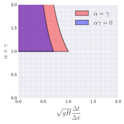
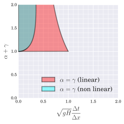
Figure 4: One-dimensional linear stability analysis: (CFL, $\alpha+\gamma$) sampling in the particular cases $\alpha=\gamma$ (red) and $\alpha\gamma=0$ (blue) at first-order in space and time (left). Comparison with the relaxed condition issuing from (25) in the case $\alpha=\gamma$ (right). Two-dimensional linear stability analysis involves a rescaling of the CFL numbers dividing them by ${\normalcolor\sqrt{2}}$.

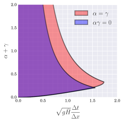
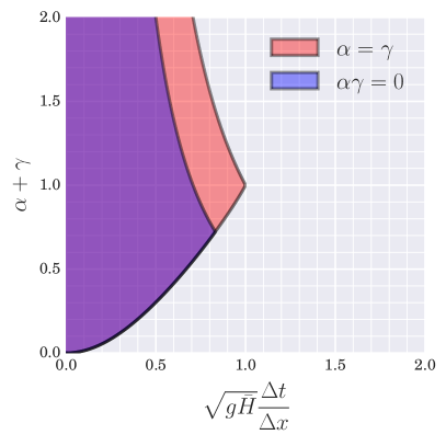
Figure 5: One-dimensional linear stability analysis: (CFL, $\alpha+\gamma$) sampling in the particular cases $\alpha=\gamma$ (red) and $\alpha\gamma=0$ (blue) with a Heun’s time stepping scheme. First-order in space (left) and second-order MUSCL reconstruction scheme in space (right). Two-dimensional linear stability analysis involves a rescaling of the CFL numbers dividing them by ${\normalcolor\sqrt{2}}$.

As concerns the increase of time and space accuracy, if it is difficult to exhibit explicit conditions based on the fully discrete model (we refer however to Appendix 7.3.3 for an extension to MUSCL schemes), some interesting results can be established in the linear case. Other series of tests were made integrating a second-order MUSCL reconstruction in space, together with the Heun’s method for time discretization (see Appendix 7.3.1 and 7.4 for implementations purposes). From a general point of view, the improvement of time order comes with the possibility of substantial practical enhancements. As regards first-order in space, the CFL can be increased and the admissible range for $\gamma$ and $\alpha$ is significantly larger, as illustrated in Fig.5 (left). In particular, $\gamma$ and $\alpha$ can both be taken arbitrarily small at the price of sufficient time step restrictions. The regularizing virtues of the second-order time algorithm are still observed when considering a MUSCL reconstruction (see Fig.5 (right)). These results are in accordance with those provided by our simulations in linear regimes (see the dedicated Section 5). These conclusions are of major interest from the extent that minimizing the diffusive losses is essential in our applicative contexts.

All the previous results can be easily extended to the two-dimensional problem. A first remarkable result is that the CFL numbers need to be rescaled dividing by $\sqrt{2}$, and not $2$ as it could be anticipated. A second result is that the $\alpha$ stabilization constant has to be two times smaller to retrieve the one-dimensional results, obtained with the corrected potential pressure stabilization term (30).

4 Asymptotic regimes

We show in this part the asymptotic preserving features of the current approach. Since the scheme reduces to a convex combination of 1d schemes (see Appendix 7.2), only the 1d case is investigated. In the one-dimensional frame, for a given time step $\Delta t$ and space step ${\Delta x}$, the numerical scheme (9a, 9b) can be interpreted at the semi-discrete level as follows:

$$H_{i}^{n+1}-H_{i}^{n} ={\displaystyle\Delta t}\partial_{x}(Hu)_{i}^{n}+\left(\Delta t\right)^{2}\gamma\partial_{x}\left(H_{i}\dfrac{\partial_{x}{\Phi_{i}}}{\varepsilon^{2}}\right)^{n}$$ (32a)

$$(Hu)_{i}^{n+1}-(Hu)_{i}^{n} =-\Delta t\left(\partial_{x}\left(\bar{u}_{i}(Hu)_{i}^{\ast}\right)\right)^{n}\vspace{1mm}$$ (32b)

$$\qquad-\Delta t\left(H_{i}\dfrac{\partial_{x}{\Phi_{i}}}{\varepsilon^{2}}\right)^{n}+\left(\Delta t\right)^{2}\alpha\left(H_{i}\dfrac{\partial_{xx}(Hu)_{i}}{\varepsilon^{2}}\right)^{n}\,,$$

where $(Hu)_{i}^{\ast}=(Hu)_{i}-\Delta t\gamma\left(H_{i}\dfrac{\partial_{x}{\Phi_{i}}}{\varepsilon^{2}}\right)$ , and $\bar{u}_{i}$ stands for the velocity $u_{i}$ perturbed with a $\mathcal{O}({\Delta x})$ viscosity term resulting from the upwind strategy on the momentum equations. Note that the space step is submitted to a classical explicit CFL condition of the form:

$$\dfrac{\Delta t}{\Delta x}\left(u+\dfrac{c}{\varepsilon}\right)\leq cste\,.$$ (33)

Of course, a fully discrete analysis can be proposed, as done in [44]. Nevertheless, at the end of the day, reformulating the scheme (9a, 9b) in terms of discrete operators in one dimension, we are left with the study of the semi-continuous scheme (32a, 32b) subject to an $\mathcal{O}(\Delta x)$ perturbation, which has no incidence on the asymptotic beahaviour. Thus, in this section, the results will be established at the continuous level in space for the sake of simplicity.

4.1 Fine time scale

For small time scale $t=\varepsilon\tau$ the model (1) degenerates toward a system of wave equations (see [51], [16]):

$$\partial_{\tau\tau}^{2}H_{i}-\mathrm{div}(H_{i}\nabla{\Phi_{i}})=0\,.$$ (34)

Theorem 4.1.

Consistency with the wave equations (34):
Consider the time step scaling $\Delta t=\varepsilon\Delta\tau$. The semi-discrete model (32a,32b) furnishes an approximation of the wave equations (34) with an error in the order of $\mathcal{O}(\Delta\tau)$.

Proof.

We drop the subscript “i” for the sake of simplicity. Using the mass equation (32a) at times $n$ and $n+1$:

$$\begin{array}[]{lllllll}H^{n+1}&-&H^{n}&=&-\varepsilon\Delta\tau\partial_{x}(Hu)^{n}&+&\left(\Delta\tau\right)^{2}\gamma\partial_{x}\left(H\partial_{x}{\Phi}\right)^{n}\,,\\ H^{n}&-&H^{n-1}&=&-\varepsilon\Delta\tau\partial_{x}(Hu)^{n-1}&+&\left(\Delta\tau\right)^{2}\gamma\partial_{x}\left(H\partial_{x}{\Phi}\right)^{n-1}\,,\end{array}$$

we write:

$$\dfrac{H^{n+1}-2H^{n}+H^{n-1}}{\left(\Delta\tau\right)^{2}}=-\dfrac{\varepsilon}{\Delta\tau}\left[\partial_{x}\left((Hu)^{n}-(Hu)^{n-1}\right)\right]+\gamma\left[\partial_{x}\left(\left(H\partial_{x}{\Phi}\right)^{n}-\left(H\partial_{x}{\Phi}\right)^{n-1}\right)\right]\,.$$ (35)

Consider now the momentum equations (32b), and multiply by $\dfrac{\varepsilon}{\Delta\tau}$:

$$\begin{split}\dfrac{\varepsilon}{\Delta\tau}\left((Hu)^{n}-(Hu)^{n-1}\right)=&-\varepsilon^{2}\left(\partial_{x}\left(\bar{u}(Hu)^{\ast}\right)\right)^{n-1}\\ &-\varepsilon^{2}\left(H\dfrac{\partial_{x}{\Phi}}{\varepsilon^{2}}\right)^{n-1}+\varepsilon\Delta\tau\alpha\left(H\partial_{xx}\left((Hu)\right)\right)^{n-1}\,.\end{split}$$ (36)

Going back to the definition of $(Hu)^{\ast}$ we write:

$$\varepsilon^{2}(Hu)^{\ast}=\varepsilon^{2}\left(Hu-\varepsilon\Delta\tau\gamma\partial_{x}\left(H\dfrac{\partial_{x}{\Phi}}{\varepsilon^{2}}\right)\right)=\underset{\varepsilon\rightarrow 0}{\mathcal{O}}(\varepsilon^{2})+\mathcal{O}(\Delta\tau)\,.$$

Since $\bar{u}_{i}$ is $\mathcal{O}(1)$, we have as a direct consequence:

$$\varepsilon^{2}\left(\partial_{x}\left(\bar{u}(Hu)^{\ast}\right)\right)=\underset{\varepsilon\rightarrow 0}{\mathcal{O}}(\varepsilon^{2})+\mathcal{O}(\Delta\tau)\,.$$

Finally, substituting (36) in (35) we obtain:

$$\dfrac{H_{i}^{n+1}-2H_{i}^{n}+H_{i}^{n-1}}{\left(\Delta\tau\right)^{2}}=\partial_{x}\left(H\partial_{x}{\Phi}\right)_{i}^{n}+\underset{\varepsilon\rightarrow 0}{\mathcal{O}}(\varepsilon^{2})+\mathcal{O}(\Delta\tau)\,,$$ (37)

that is the one-dimensional equivalent of (34) with an error in the order of $\Delta\tau$ and a second-order perturbation.∎

4.2 Large time scale

Assuming the Hessian ${\boldsymbol{\mathcal{H}}}$ (6) well-conditioned with respect to $\varepsilon$, that is the condition number of ${\boldsymbol{\mathcal{H}}}$ is $\underset{\varepsilon\rightarrow 0}{\mathcal{O}}(1)$, the asymptotic regime associated with large time scales $t=\underset{\varepsilon\rightarrow 0}{\mathcal{O}}(1)$ can be derived as a divergence-free model:

$$\left\{\begin{aligned} \mathrm{div}\left(H\textbf{u}_{i}\right)&=0\,\\ \partial_{t}\textbf{u}_{i}+\left(\textbf{u}_{i}.\nabla\right)\textbf{u}_{i}&=-\nabla\Phi_{i}\end{aligned}\right.\,.$$ (38)

Theorem 4.2.

Consistency with the divergence free model (38):
Consider the time step scaling $\Delta t=\underset{\varepsilon\rightarrow 0}{\mathcal{O}}(1)$, and assume that the spatial perturbation of the potential is in the order of $\varepsilon^{2}$:

$$\Phi_{i}(t,x)=\bar{\Phi}_{i}(t)+\varepsilon^{2}\hat{\Phi}_{i}(t,x)\,.$$ (39)

Then the semi-discrete model (32a,32b) furnishes an approximation of the wave equations (38) with an error in the order of $\mathcal{O}(\Delta t)$ and $\mathcal{O}(\Delta t,{\Delta x})$ respectively.

Proof.

Note that with (39), and based on the regularity assumptions made on the potential forces (2.1), we also have:

$$\partial_{t}\Phi_{i}=\underset{\varepsilon\rightarrow 0}{\mathcal{O}}(\varepsilon^{2})\qquad\text{ and }\qquad\partial_{t}H_{i}=\underset{\varepsilon\rightarrow 0}{\mathcal{O}}(\varepsilon^{2})\,.$$

Again, we drop the subscript “i” to alleviate the notations. We directly obtain from (32a):

$$\partial_{x}\left(Hu^{\ast}\right)^{n}=\partial_{x}\left(Hu\right)^{n}-\Delta t\gamma\partial_{x}\left(H\partial_{x}\hat{\Phi}\right)^{n}=\underset{\varepsilon\rightarrow 0}{\mathcal{O}}(\varepsilon^{2})\,,$$ (40)

that is the divergence-free condition with an error in $\mathcal{O}(\Delta t)$ and a second-order perturbation. Using the relation:

$$(Hu)^{n+1}-(Hu)^{n}=\left(H^{n+1}-H^{n}\right)u^{n+1}+H^{n}\left(u^{n+1}-u^{n}\right)=H^{n}\left(u^{n+1}-u^{n}\right)+\underset{\varepsilon\rightarrow 0}{\mathcal{O}}(\varepsilon^{2})\,,$$

together with the momentum equation (32b) we write:

$$\dfrac{u^{n+1}-u^{n}}{\Delta t}=-\dfrac{1}{H^{n}}\left(\partial_{x}\left(\bar{u}(Hu)^{\ast}\right)+\left(H\partial_{x}\hat{\Phi}\right)\right)^{n}+\Delta t\alpha\left(\dfrac{\partial_{xx}\left(Hu\right)^{n}}{\varepsilon^{2}}\right)+\underset{\varepsilon\rightarrow 0}{\mathcal{O}}(\varepsilon^{2})\,.$$ (41)

For any $n$, we first note that:

$$\begin{split}\dfrac{1}{H}\partial_{x}\left(\bar{u}(Hu)^{\ast}\right)&=u\partial_{x}u+\underset{\varepsilon\rightarrow 0}{\mathcal{O}}(\varepsilon^{2})+\mathcal{O}(\Delta t,{\Delta x})\end{split}$$ (42)

going back to the semi-discrete divergence free relation (40), one has:

$$\begin{split}\partial_{xx}\left(Hu\right)=\Delta t\gamma\partial_{xx}\left(H\partial_{x}\hat{\Phi}\right)+\underset{\varepsilon\rightarrow 0}{\mathcal{O}}(\varepsilon^{2})\,,\end{split}$$ (43)

and hence:

$$\Delta t\alpha\left(\dfrac{\partial_{xx}\left(Hu\right)}{\varepsilon^{2}}\right)=\left(\dfrac{\Delta t}{\varepsilon}\right)^{2}\alpha\gamma\partial_{xx}\left(H\partial_{x}\hat{\Phi}\right)+\mathcal{O}(\Delta t)\,.$$ (44)

Under the explicit CFL (33), the first term of the right hand side is $\mathcal{O}({\Delta x}^{2})$. At last this gives:

$$\dfrac{u_{i}^{n+1}-u_{i}^{n}}{\Delta t}=-u_{i}\partial_{x}u_{i}-\partial_{x}\hat{\Phi}_{i}+\underset{\varepsilon\rightarrow 0}{\mathcal{O}}(\varepsilon^{2})+\mathcal{O}(\Delta t,{\Delta x})\,.$$ (45)

∎

5 Numerical test cases

This part is dedicated to the survey of the numerical scheme’s global efficiency at first and second-order, with a particular focus on low Froude regimes. Theoretical and numerical investigations involving wet/dry fronts and a complex management of the layers are left for future works. For the sake of completeness, the second-order extension in space and time, the adaptive time step used and the time stepping scheme to incorporate the Coriolis force are given in the Appendix 7. We recall here that all the numerical tests were performed with $\widehat{H}_{K}^{n}=H_{K}^{n}$ in the numerical fluxes (10a, 11, 14) (see Remarks 2.4 and 3.7).

It should be emphasized that it is difficult to carry on qualitative comparisons on the different numerical approaches in case of multiple layers. This is mainly due to the very small number of such academic test cases available in the literature, as it is difficult to derive analytical solutions. Some reference solutions for the multilayer shallow water model with the Coriolis force are of course provided by more sophisticated operational softwares like HYCOM [11], ROMS [49] or NEMO [37], but with the inconvenience of not being necessary exactly based on the same physical model as the one concerned here.

A first academic test case is considered, involving two-dimensional oscillating layers around a steady state in the linear small amplitude limit. It is investigated for this test case the inequality conditions for the stabilization constants $\gamma$ and $\alpha$ ensuring the linear stability, as well as those which guarantee the strict decrease of the mechanical energy between each time step. At the end, the a priori best pair verifying the two stability conditions with a minimum of dissipation will be extracted and the resulting scheme compared to the classical HLLC approximate Riemann solver (see [55] with the wave speed estimates of [57]). In a second test case, the scheme’s accuracy is investigated for a smooth two-dimensional, non-stationnary and non-linear solution. In a third test case, we focus on the well-balanced property, considering an initial jump of water surface elevation propagating over a non trivial topography. A more advanced test case is finally studied, the so-called baroclinic vortex, that can be found in the COMODO benchmark [1], a test suite set up by the international oceanographic community to evaluate and compare the numerical solvers efficiency.

5.1 Linear waves

In the present test case we investigate the two-dimensional simulation of oscillating layers around a steady state of flat layers with a flat bottom. In case of waves of small amplitude, an approximate analytical solution can be derived from the linear wave theory. Considering only one layer, in the limit of small amplitude variation around the layer depth at rest $\eta_{0}$, the deviation $\zeta_{1}$ ($\eta_{1}=\eta_{0}+\zeta_{1}$) is solution of the two-dimensional wave equation with the associated dispersive relation $\omega^{2}=c^{2}\left(k_{x}^{2}+k_{y}^{2}\right)$, where $k_{x}$ and $k_{y}$ are the wave numbers in the $x$ and $y$ direction respectively. Considering now the same problem for the $L$ layers shallow water model, we obtain $L$ coupled linear wave equations,

$$\forall i\in\left\llbracket 1,L\right\rrbracket,\quad{\displaystyle\frac{\partial^{2}\zeta_{i}}{\partial t^{2}}-c_{i}^{2}\sum_{j=1}^{L}\frac{min(\rho_{i},\rho_{j})}{\rho_{i}}\triangle\zeta_{j}=0}\,.$$

By denoting $\tilde{c}_{i}$ the eigenvalues of the matrix ${\displaystyle A_{ij}=\left(c_{i}^{2}\frac{\min(\rho_{i},\rho_{j})}{\rho_{i}}\right)}$, the above coupled system of wave equations can be rewritten in $L$ uncoupled linear wave equations,

$$\forall i\in\left\llbracket 1,L\right\rrbracket,\quad{\displaystyle\frac{\partial^{2}\tilde{\zeta}_{i}}{\partial t^{2}}-\tilde{c}_{i}^{2}\triangle\tilde{\zeta}_{i}=0}\,,$$

where $\tilde{\zeta}$ is the projection of $\zeta$ onto the diagonal basis using the left eigenvectors matrix. Simulations are initialized in a $100\ \mathrm{km}$ square box with periodic boundary conditions, a sea surface at rest $\eta{}_{0}=5000\ \mathrm{m}$, five evenly spaced layers $h_{i}=1000\ \mathrm{m}$ with densities following a linear law $\rho_{i}=1000+50\>(i-1)$ and a gravitational acceleration $g=10\ \mathrm{m}.\mathrm{s}^{-2}$. Note that the density ratios considered here, large in comparison with those encountered in more realistic contexts like oceans, have the effect of reducing the wave phase speed differences and allowing to consider a smaller time integration to capture the layers interaction. Considering a deviation $\zeta_{1}=\cos\left(k_{x}x\right)\cos\left(k_{y}y\right)$ only for the first layer with one wavelength in each direction, approximatively $11$ wave periods can be observed with a simulation time $t=3600\>\mathrm{\mathrm{s}}$ for a maximum wave velocity $\max\left(\tilde{c_{i}}\right)\approx\sqrt{2gh_{0}}\approx 316\ \mathrm{m}.\mathrm{s}^{-1}$. We give here the expression of the discrete mechanical energy:

$${\normalcolor E^{n}={\displaystyle\frac{1}{2}}{\displaystyle\sum_{K\in\mathbb{T}}\sum_{i=1}^{L}m_{K}\frac{\rho_{i}}{\rho_{L}}\left(h_{K,i}^{n}\left\|\mathbf{u}_{K,i}^{n}\right\|^{2}/\epsilon^{2}+g\left(h_{K,i}^{n}\right)^{2}+2\sum_{j=i+1}^{L}gh_{K,i}^{n}h_{K,j}^{n}\right)}}\,,$$ (46)

as it will be a useful measurement for the simulations presented above. Note finally that $\epsilon=2.10^{-4}$ for this test, giving a very low Froude solution.

5.1.1 Stability issues - searching for optimal stabilization parameters

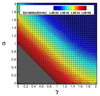
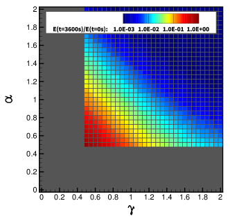
Figure 6: Mechanical energy dissipation according to $\gamma$ and $\alpha$ with a fixed CFL number of $0.5$ in (98) using the first-order scheme and a $41\times 41$ mesh size ; (left) gray zone corresponds to an unstable algorithm ; (right) gray zone corresponds to a non monotonically decreasing energy. The energy ratio $E(t=3600\,\mathrm{s})/E(t=0\,\mathrm{s})$, computed from (46) and displayed in $log$ scale, highlights the scheme’s dissipation.

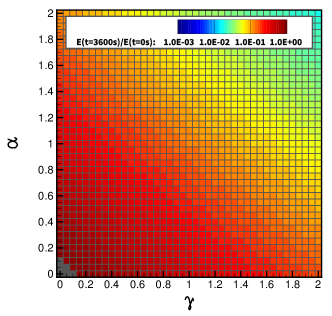
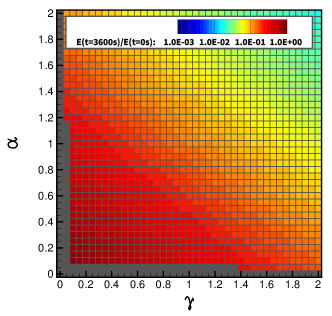
Figure 7: Mechanical energy dissipation according to $\gamma$ and $\alpha$ with a fixed CFL number of $0.5$ in (98) using the second-order scheme and a $11\times 11$ mesh size; (left) gray zone corresponds to an unstable algorithm; (right) gray zone corresponds to a non monotonically decreasing energy. The energy ratio $E(t=3600\,\mathrm{s})/E(t=0\,\mathrm{s})$, computed from (46) and displayed in $log$ scale, highlights the scheme’s dissipation.

A preliminary goal for this test case is to search numerically a range for the two stabilization constants $\gamma$ and $\alpha$ that ensures linear stability, and another that ensures a strict decrease of mechanical energy, while aiming at minimizing the dissipation, for a CFL number arbitrarily fixed at $0.5$ in (98). In order to address that question, thousands of numerical simulations have been performed with regular variations of the two constants (with a $0.05$ step), testing for each pair two stopping criteria separately during the simulation. The first one, intented to detect a possible breaking point in the linear stability of the scheme, is based on an a priori exponential growth of the mechanical energy and the second one, more restrictive, checks if the mechanical energy decrease is violated at each time step. These experiments were carried out using a $41\times 41$ mesh size for the first-order scheme (9a-9b-10a-10b) and a $11\times 11$ mesh size for the second-order scheme (Eqs.83). These mesh sizes allow to keep the same order of magnitude for the mechanical energy diffusion. All the numerical results are summarized for the first-order scheme in Fig.6 and for the second-order scheme in Fig.7.

For the first criterion, it can be clearly observed for the first-order scheme that the sum $\gamma+\alpha$ must be greater than a minimum value of $1$. This result is perfectly consistent with the linear stability analysis presented in §3.4, in the sense that the sum ${\normalcolor\gamma+\alpha}$ governs the terms of the amplification matrix, while the product $\gamma\alpha$ is marginal. As one could expect, it is also found a minimum of dissipation for this minimal sum value. Notice that one of the two coefficients can be taken to zero and that the minimum of dissipation is reached for $\gamma=1$ and $\alpha=0$. Greater sum values introduce quickly and nearly proportionally large amounts of dissipation. For the second-order scheme, the same general behaviour is observed again, except that the minimum sum value found is now $0.15$, really much lower than for the first-order case. But in contrast with the first-order scheme, this value is correlated to the given CFL number of $0.5$. This result may be perceived unintuitive because MUSCL reconstructions tends to reduce the value of the stabilization terms appearing in the mass flux and the pressure term (84) for very regular solutions. We have verified in the linear stability analysis that this is the Heun’s method for time discretization which mainly explains this reduction, changing profoundly the diffusion terms nature. The increase of dissipation induced by greater sum values is also much more limited compared to the first-order scheme.

If we now look to the second criterion, based on the mechanical energy strict decrease, the two coefficients must be both greater than a minimum value of $0.5$ for the first-order scheme, and a minimum value of $0.15$ for the second-order scheme, except for too high inefficient stabilization constants exhibiting more dissipation. This experiment confirms an important result: the two stabilization constants $\gamma$ and $\alpha$ are both necessary to find a strict mechanical energy decrease.

The stability condition inequalities found for this test case of fast gravitational waves are summarized in Tab.1. It is found optimal stabilization constants $\gamma=0.5$ and $\alpha=0.5$ for the first-order scheme and $\gamma=0.1$ and $\alpha=0.1$ for the second-order scheme if the CFL number is fixed to $0.5$. Many other simulations were run in other contexts, without bringing any significant variability on these conditions.

first-order scheme (independant of the CFL)
linear stability	mechanical energy dissipation
$\gamma+\alpha\geq 1$	$\gamma\geq 0.5$ and $\alpha\geq 0.5$
second-order scheme (only for a CFL number of 0.5 in (98))
linear stability	mechanical energy dissipation
$\gamma+\alpha\geq 0.15$	$\gamma\geq 0.1$ and $\alpha\geq 0.1$

Table 1: Stability inequalities conditions found by a numerical experiment of two-dimensional gravity waves for the first and second-order schemes. The relaxed conditions obtained at second-order highlight the stabilizing effects of the Heun’s time discretization method.

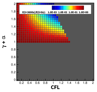
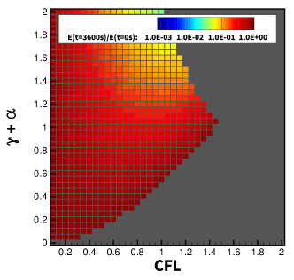
Figure 8: Mechanical energy dissipation according to the sum $\gamma+\alpha$, fixing the relation $\gamma=\alpha$, and the CFL number. Zones corresponding to an unstable algorithm and non monotonically decreasing energy are perfectly overlapping and appear in gray; (left) using the first-order scheme and a $41\times 41$ mesh size; (right) using the second-order scheme and a $11\times 11$ mesh size. The energy ratio $E(t=3600\,\mathrm{s})/E(t=0\,\mathrm{s})$, computed from (46) and displayed in $log$ scale, highlights the scheme’s dissipation.

A similar experiment was performed considering varying values for the sum $\gamma+\alpha$, fixing the relation $\gamma=\alpha$, and CFL numbers. The numerical results are summarized in Fig.8. First, without any surprise, we recover the same patterns as those from the linear stability analysis (see Figs.4 and 5 rescaling the CFL numbers). Now, an additionnal result is that the mechanical energy is also dissipated in the domains of linear stability. Secondly, for the first-order scheme, the dissipation is reduced considering smaller CFL numbers for a given sum. For the second-order scheme, the dissipation dependence with respect the CFL number is more complicated and it is not so clear how to extract an optimal pair of stabilization constants.

5.1.2 Comparison with analytical solution

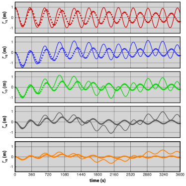
Figure 9: Time evolution of the five surface layers deviation ($\eta_{i}=\eta_{i,0}+\zeta_{i}$) at the box center computed with a $11\times 11$ mesh size. Analytical solution is given in continuous line and numerical solution in dotted line; (left) using the first-order scheme with $\gamma=\alpha=0.5$ and a CFL number of $0.5$; (right) using the second-order scheme with $\gamma=\alpha=0.1$ and a CFL number of $0.5$.

In Fig.9 we propose the time evolution of the five surface layers deviation using the first-order scheme with $\gamma=\alpha=0.5$ (left) and the second-order scheme with $\gamma=\alpha=0.1$ (right), corresponding to the two optimal pairs found in the previous section for a $0.5$ CFL number. The dispersive behaviour of the scheme can clearly be observed because of the obvious phase shift, although this effect is reduced by the second-order scheme. Nevertheless, the scheme at first and second-order reproduces qualitatively very well the multiple interactions between the layers in light of the $11\times 11$ coarse mesh size used. For this resolution and these stabilization constants, the second-order scheme does exhibit a minimum of dissipation, only the dispersive effects can be clearly distinguished.

5.1.3 Comparison with the HLLC scheme

We have found by a numerical experiment the optimal pairs of stabilization constants $\gamma$ and $\alpha$ for the first and second-order schemes. As the present method also applies to the classical shallow water equations ($L=1$), it is interesting to illustrate the current approach efficiency comparing it with other classical Godunov-type solvers. From this perspective, we reduce the present test to the one layer case, and employ the HLLC scheme, supplemented with a second-order MUSCL reconstruction coupled with the Heun’s method for time discretization.

Some numerical results are given in Fig.10. As a first remark, the original HLLC scheme totally fails to capture numerically the oscillations after a few wavelengths. There is no more mechanical energy at the end of the simulation for the majority of the mesh sizes considered here. An extreme level of refinement is needed to asymptotically capture the first-order convergence. The problem is however significantly reduced employing the second-order extension in space and time.

With regard to the presented scheme, the results are widely better than for the HLLC scheme at first and second-order. As a matter of fact, the first-order scheme is already better than the second-order HLLC scheme, while bearing in mind that the computational cost is in addition really smaller. Note that with this level of refinement, a third order convergence rate is reached for the first-order scheme, except for most refined meshes, which may indicate a progressive alignment on the right order of convergence. The present second-order scheme does not exhibit significant losses of mechanical energy. Only a phase shift is observed, introduced by the dispersive nature of the flow, in the same order of magnitude than the HLLC scheme.

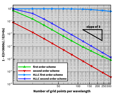
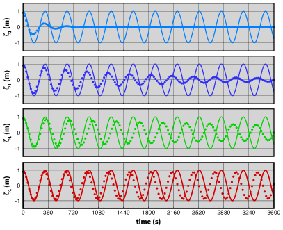
Figure 10: Comparison with the HLLC scheme in the one-layer case; (left) Mechanical energy dissipation for varying numbers of grid points per wavelength for the present scheme and the HLLC scheme, at first and second-order. (right) Evolution of surface level at the box center for a $11\times 11$ mesh size with analytical solution in continuous line and numerical solution in dotted line; (from top to bottom) first-order HLLC scheme, second-order HLLC scheme, present first-order scheme with $\gamma=\alpha=0.5$ and present second-order scheme with $\gamma=\alpha=0.1$, all with a $0.5$ CFL number.

5.2 Smooth surface wave propagation

We investigate here the numerical scheme’s accuracy for a smooth two-dimensional, non-stationnary and non-linear solution. To this end, a water depth Gaussian profile is placed in the bottom-left corner of a $500\ km$ square domain with prescribed slip boundaries:

$$\left\{\begin{array}[]{l}h(x,y,t=0)=h_{0}+h_{1}e^{{\displaystyle-r^{2}/2\sigma^{2}}}\\ \mathbf{u}(x,y,t=0)=\mathbf{0}\end{array}\right.,$$ (47)

where $r$ is the radial coordinate, $h_{0}=5000\ \mathrm{m}$, $h_{1}=10\ \mathrm{m}$ and $\sigma=50\ \mathrm{km}$. We consider a flat bottom and a gravitational acceleration $g=10\ m.s^{-2}$. Considering a simulation time $t=600\>\mathrm{s}$, a reference solution is generated using a $2560\times 2560$ mesh and the second-order HLLC scheme. Varying the meshes from $10^{2}$ to $320^{2}$ cells, the $L^{2}$ absolute error norm between the numerical and reference solutions (integrating it for each cell of the coarser mesh) are computed at the end of the simulation. The results given in Tab.2 are first showing that the expected orders of convergence are asymptotically reached. Note the remarkable hierarchy for a given mesh size regarding the computed error norm: the first-order HLLC scheme, the first-order present scheme, the HLLC scheme with a Heun/MUSCL second-order extension and the present second-order scheme with the same extension. The present second-order scheme provides the smallest error norm independently of the mesh size, except for the most refined cases where the result is identical to the second-order HLLC scheme. The asymtotic convergence to second-order is consequently more rapid for the HLLC scheme for this test. Finally, the numerical solutions along the radial coordinate computed with a coarse $20^{2}$ mesh for the four schemes are given in Fig.11, highlighting that our first-order method is qualitatively as efficient as a second-order HLLC scheme.

$n_{x}\times n_{y}$	$\epsilon_{L_{2}}$	order		$n_{x}\times n_{y}$	$\epsilon_{L_{2}}$	order
HLLC first-order scheme				present first-order scheme ($\alpha=\gamma=0.5$)
$10^{2}$	$3.18\>10^{-1}$	-		$10^{2}$	$2.25\>10^{-1}$	-
$20^{2}$	$2.27\>10^{-1}$	$0.49$		$20^{2}$	$1.11\>10^{-1}$	$1.02$
$40^{2}$	$1.42\>10^{-1}$	$0.68$		$40^{2}$	$3.76\>10^{-2}$	$1.56$
$80^{2}$	$8.07\>10^{-2}$	$0.82$		$80^{2}$	$1.42\>10^{-2}$	$1.40$
$160^{2}$	$4.34\>10^{-2}$	$0.90$		$160^{2}$	$6.25\>10^{-3}$	$1.18$
$320^{2}$	$2.26\>10^{-2}$	$0.94$		$320^{2}$	$2.99\>10^{-3}$	$1.06$
HLLC second-order scheme				present second-order scheme ($\alpha=\gamma=0.1$)
$10^{2}$	$1.69\>10^{-1}$	-		$10^{2}$	$1.16\>10^{-1}$	-
$20^{2}$	$6.64\>10^{-2}$	$1.35$		$20^{2}$	$4.70\>10^{-2}$	$1.30$
$40^{2}$	$1.87\>10^{-2}$	$1.83$		$40^{2}$	$1.72\>10^{-2}$	$1.45$
$80^{2}$	$4.78\>10^{-3}$	$1.97$		$80^{2}$	$4.67\>10^{-3}$	$1.87$
$160^{2}$	$1.21\>10^{-3}$	$1.98$		$160^{2}$	$1.21\>10^{-3}$	$1.96$
$320^{2}$	$2.99\>10^{-4}$	$2.02$		$320^{2}$	$3.00\>10^{-4}$	$2.01$

Table 2: Numerical convergence results for the radial smooth surface wave propagation. The errors $\epsilon_{L^{2}}$ refer to the absolute $L^{2}$ norm between the computed numerical solution obtained with a $n_{x}\times n_{y}$ mesh size and the reference solution computed with a $2560\times 2560$ mesh size.

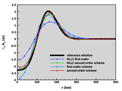
Figure 11: Numerical results for the radial smooth surface wave propagation obtained at time $t=600\>\mathrm{s}$ along one radial axis computed with a $20\times 20$ mesh size.

5.3 Small perturbation of a lake at rest

This test case proposed in [34] and reproduced for example in [43], [48] and [53] is intended to check the scheme’s ability to deal both with the well-balanced property and the propagation of a jump in the initial water surface elevation. It should be recalled that the first-order scheme is well-balanced by construction and that this property easily extends to the second-order MUSCL reconstruction scheme, as it has been discussed in §3.1.

This test involves a two-dimensional rectangular computational domain $\left[0,2\right]\times\left[0,1\right]$ and a non linear topography at the bottom:

$$z_{b}=0.8\>e^{{\displaystyle\left(-5\left(x-0.9\right)^{2}-50\left(y-0.5\right)^{2}\right)}}.$$ (48)

First, considering an initial motionless constant water surface elevation $\eta_{1}=1$, the solution should stay at rest. At first and second-order in space, it is found that whatever the simulation time is, the water surface elevation and velocity error norms are exactly zero because of the exact flux balance with respect to the discrete potential.

Next, following the original test case in [34], we consider a jump of water surface elevation:

$$\eta_{1}(x,y,t=0)=\left\{\begin{array}[]{ll}1.01&\text{if }0.05\leq x\leq 0.15\\ 1&\text{otherwise}\end{array}\right..$$ (49)

Slip boundaries are prescribed except an idealized outflow at western boundary, considering an extended computational domain to avoid any reflexion, as the initial water surface bump generates left- and right-going waves. Considering a simulation time $t=0.46\>s$, some snapshots are given in Fig.12 for the present scheme, at first and second-order for a relatively coarse $300\times 100$ mesh (bottom). Using the same resolution, these results can be compared with the second order HLLC scheme, and an highly resolved solution, serving as reference (top). A Barth limiter [7] has been used for the reconstructed water surface elevation to prevent from too much dispersive solutions. Our scheme is reproducing qualitatively very well the complex flow dynamics. However, notably due to the discontinuous nature of the initial solution, the stabilization constants must be taken higher than the optimal ones found in the previous test case (Tab.1) to avoid spurious oscillations. Cross sections of the final solution are displayed in Fig.13, showing again a low level of numerical diffusion in comparison with the classical HLLC scheme. In conclusion, our scheme can be succesfully employed for this kind of complex flows, implying an initial jump and non trivial topography. These observations also tend to indicate that the scheme’s efficiency can be significantly improved with an adjustment of the constants $\gamma$ and $\alpha$, according to the local regularity of the discrete solution. Additional theoretical and numerical investigations are currently in progress in that direction.

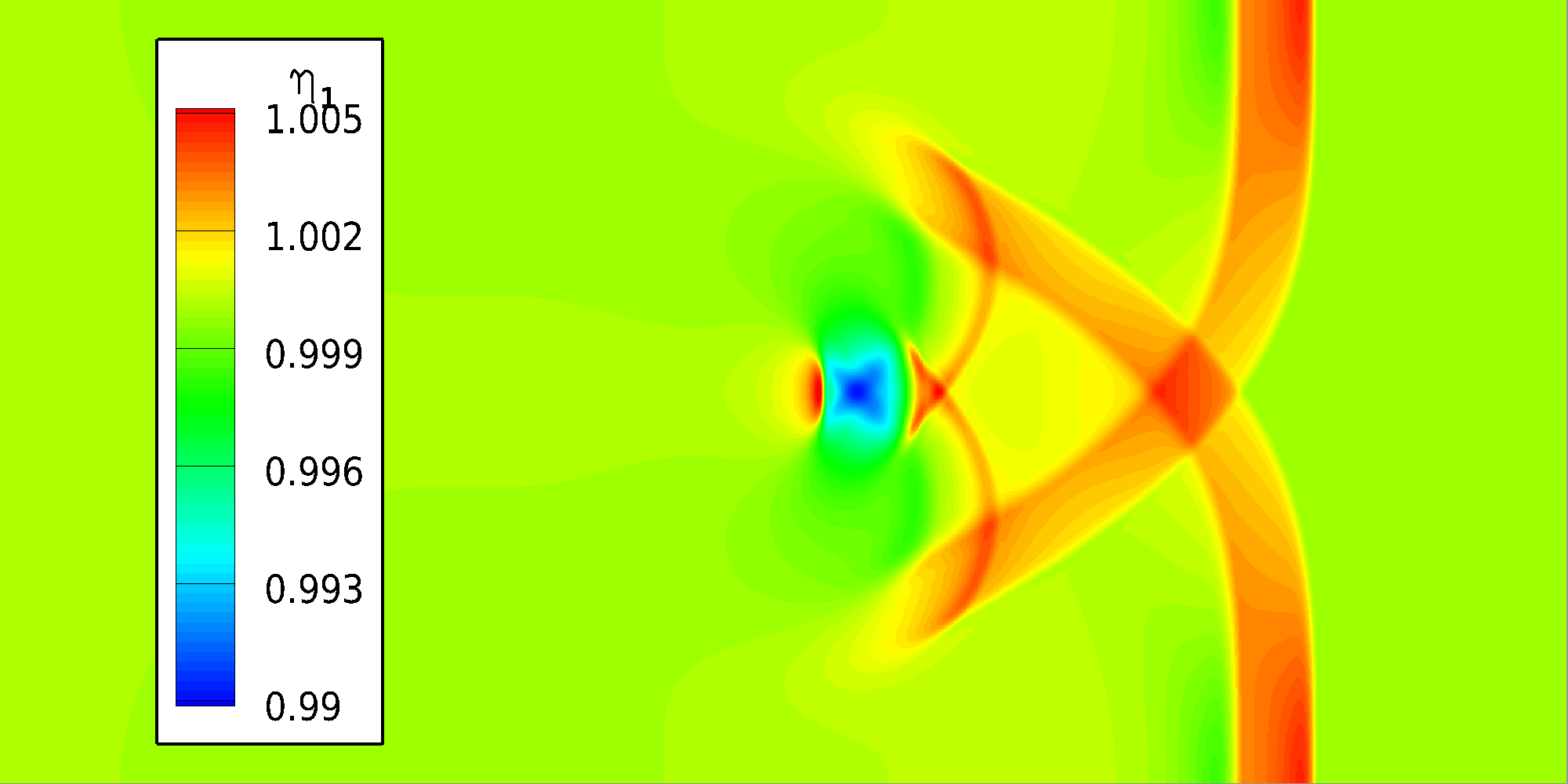
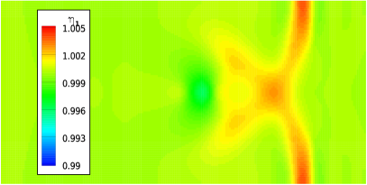
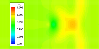
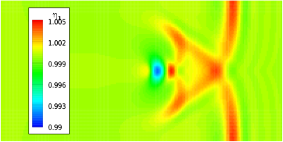
Figure 12: Numerical simulations of a propagating wave considering the bottom topography (48) and the initial condtion (49); water surface top view at time $t=0.46\>s$; (top) using the second-order HLLC scheme and a $1600\times 800$ mesh size (left), and a $300\times 100$ mesh size (right); (bottom) using a $300\times 100$ mesh size and the present first-order scheme with $\gamma=\alpha=1$ (left) and the present second-order scheme with $\gamma=\alpha=0.5$ (right).

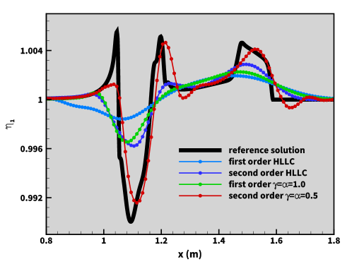
Figure 13: Slides view corresponding to the simulations in Fig.12 along the horizontal axis at the middle of the domain, at time $t=0.46\>s$ and for a $300\times 100$ mesh. A Barth limiter [7] has been used for the MUSCL reconstructed water surface elevation.

5.4 Baroclinic vortex

Based on the COMODO benchmark [1], we study here an idealized axisymmetric and anticyclonic baroclinic vortex initially centered, propagating south-westward due to a $\beta$-plane approximation, following the numerical experiment proposed in [45]. The vortex is expected to approximately retains its axisymmetric shape with a progressive decrease of energy along its trajectory, mainly in the wave of emissions of weak-amplitude Rossby-waves. This last test case represents a good indicator of the scheme’s accuracy in the frame of a complex flow with several layers, the principal difficulty lying in the capability to describe accurately the vortex motion. Indeed, the numerical diffusion and dispersion induced by unsuitable schemes can quickly break the cyclostrophic balance and subsequently deteriorate the vortex trajectory.

5.4.1 Initialization

A vortex is placed at the center of the box $\left[-900\ \mathrm{km},900\ \mathrm{km}\right]^{2}$ with boundary walls according to an axisymmetric Gaussian pressure profile:

$$\begin{array}[]{l}\eta_{1}={\displaystyle\frac{P_{0}}{g\rho_{0}}}e^{\nicefrac{{-r^{2}}}{{2\lambda^{2}}}}\end{array}\,,$$ (50)

where $\rho_{0}=1024.4\ \mathrm{kg}.\mathrm{m}^{-3}$ is the density at sea surface, $g=9.81\ \mathrm{m}.\mathrm{s}^{-2}$ is the gravitational acceleration, $\lambda=60\ \mathrm{km}$ and $P_{0}=\rho_{0}f_{0}u_{max}\lambda\sqrt{e}$ is a pressure defined from a maximum velocity $u_{max}=0.8\ \mathrm{m}.\mathrm{s}^{-1}$, giving an anticyclonic vortex. In each layer $i$, the vortex at cyclostrophic equilibrium respects an axisymmetric balance between centripetal acceleration $v_{i,\theta}$, pressure $p_{i}$ and Coriolis force:

$$-{\displaystyle\frac{v_{i,\theta}^{2}}{r}}-fv_{i,\theta}+{\displaystyle\frac{dp_{i}}{dr}}=0\,.$$ (51)

Eliminating the unphysical solution, we obtain the final velocity expression in each layer as a function of the layer pressure gradient in cylindrical coordinates:

$$v_{i,\theta}=-{\displaystyle\frac{fr}{2}}\left(1-\sqrt{1+{\displaystyle\frac{4{\displaystyle\frac{dp_{i}}{dr}}}{rf^{2}}}}\right)\,.$$ (52)

Note that with simulations initialized with a velocity at geostrophic equilibrium $v_{i,\theta}={\displaystyle-\frac{1}{f}\frac{dp_{i}}{dr}}$ as prescribed in the original test case [1], numerical approximations generates too much undesirable small scale waves because of the initial imbalance at the continuous level (ignoring the $\beta$-plane approximation). As their wavelength decreases with the mesh size, and as we have seen that our scheme does not dissipate high frequencies, it involves an improper convergence. As a consequence, the $u_{max}$ considered here is smaller than in the original test case to ensure the positivity of the term in the square root in (52).

A $\beta$-plane approximation is made for the Coriolis force:

$$\begin{array}[]{l}f=f_{0}+\beta y\end{array}\,,$$ (53)

with a latitude $\theta=38.5\text{\textdegree}$, giving the two constants $f_{0}=2\Omega\sin\left(\theta\right)\simeq 9,054\ 10^{-5}$ and $\beta=2\Omega\cos\left(\theta\right)/R_{earth}\simeq 1,788\ 10^{-11}$. The density distribution involves ten layers at rest, evenly sized, following the linear law:

$$\begin{array}[]{l}\rho_{i}=\rho_{0}\left(1-{\displaystyle\frac{N^{2}}{g}z_{i}}\right)\end{array}\quad\text{with}\quad z_{i}={\displaystyle\frac{h_{0}\left(i-\frac{1}{2}\right)}{N}}\,,$$ (54)

where $N=3.10^{-3}\ \mathrm{s}^{-1}$ is the Brunt-Väisälä frequency and $h_{0}=5000\ \mathrm{m}$ is the unperturbed sea surface height. No motion is prescribed under a level $h_{1}=2500\ \mathrm{m}$ in order to prevent from fast barotropic modes as prescribed in the original test case [1]. It is derived here a formal way to nullify the velocity starting from the 6th layer. For a $L$ layers system, the potential in the layer $i$ can be written:

$$\Phi_{i}={\displaystyle\frac{g}{\rho_{i}}}\left({\displaystyle\rho_{1}\eta_{1}+\sum_{k=2}^{i}\left(\rho_{k}-\rho_{k-1}\right)\eta_{k}}\right)\,.$$ (55)

If we suppose $\nabla\Phi_{i}=0$, it can be found that:

$$\rho_{1}\nabla\eta_{1}+{\displaystyle\sum_{k=2}^{i}\left(\rho_{k}-\rho_{k-1}\right)\nabla\eta_{k}}=0\,.$$ (56)

If we suppose in addition that $\forall k>i\>,\>\nabla\eta_{k}=0$, then we find also $\forall k>i\>,\>\nabla\Phi_{k}=0$. Suppose now that $\nabla\eta_{k+1}=r\nabla\eta_{k}$, then:

$$\rho_{1}\nabla\eta_{1}+\nabla\eta_{2}{\displaystyle\sum_{k=2}^{i}\left(\rho_{k}-\rho_{k-1}\right)r^{k-2}}=0\,,$$ (57)

giving the final expression for the water surface elevation gradient:

$$\nabla\eta_{i}=\frac{-\rho_{1}r^{i-2}\nabla\eta_{1}}{{\displaystyle\sum_{k=2}^{i}\left(\rho_{k}-\rho_{k-1}\right)r^{k-2}}}\,.$$ (58)

from which we extract the final water surface elevation distribution with $r=1$ adding the layer level at rest as a constant. Let us notice the inverse sign of the internal layer gradients compared to the sea surface gradient $\nabla\eta_{1}$ (since $\rho_{k}>\rho_{k-1}$), implying a pressure gradient decrease. Finally, we recall that we do not consider any viscosity or bottom friction effects in this test case. Note finally that $\epsilon\thickapprox 3.6\>10^{-3}$ for this test case.

5.4.2 Simulations

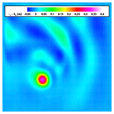
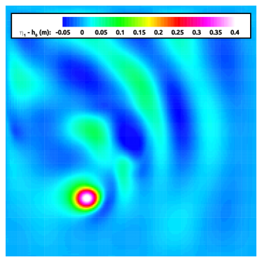
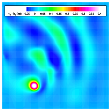
Figure 14: Sea surface height for the baroclinic vortex test case obtained with the present second-order scheme. After 100 days of simulation, the vortex, initially centered, has moved to the southwest and small amplitudes Rossby waves emission can be observed in the trajectory wake; (top-left) $\Delta x=30\ \mathrm{km}$; (top-right) $\Delta x=20\ \mathrm{km}$; (bottom-left) $\Delta x=10\ \mathrm{km}$; (bottom-right) $\Delta x=5\ \mathrm{km}$.

Simulations have been performed using the second-order scheme presented in the Appendix 7.3 with a time integration period of $100$ days with five space resolutions $\Delta x=30\,\mathrm{km}\,,\,20\,\mathrm{km}\,,\,10\,\mathrm{km}\,,\,5\,\mathrm{km}\;\text{and}\;2\,\mathrm{km}$ corresponding respectively to discretizations of space domain with $60\times 60\times 10\,,\,90\times 90\times 10\,,\,180\times 180\times 10\,,\,360\times 360\times 10\;\text{and}\;900\times 900\times 10$ cells and layers. It has been chosen $\gamma=0.2$ and $\alpha=0$ for the stabilization constants coefficients, with a CFL number of $0.5$. We have seen before that this set of parameters is sufficient to ensure the linear stability of the numerical scheme §3.4.

The sea surface height for the first four resolutions are given in Fig.14. It can be roughly observed a relative rapid convergence since the solutions for the $10\,\mathrm{km}$ and $5\,\mathrm{km}$ resolutions are already very close. The vortex final shape as well as the position and amplitude of the Rossby waves in the trajectory wake are very similar, excepted maybe for very fine structures. For the lower resolutions of $30\,\mathrm{km}$ and $20\,\mathrm{km}$, the final axisymmetric vortex shape has not been completely broken, resulting to relatively acceptable simulations. The large structures of the emitted Rossby waves are correctly captured, especially the two bands in the northeast. However, the vortex has clearly lost an important energy as its maximum amplitude is lower than for the more refined meshes.

Going further in the convergence analysis, it is given in Fig.15 the time evolution of the vortex $y$-deviation (computed from the maximum amplitude with bilinear interpolation), the vortex maximum amplitude, the kinetic and mechanical energies, obtained from (46) (substracting to the potential energy the unperturbed state contribution, the mechanical energy has been rescaled to the initial value). The overall results for the $5\,\mathrm{km}$ and $2\,\mathrm{km}$ are sufficiently close to consider that the convergence has been very nearly reached. The $2\,\mathrm{km}$ resolution exhibits a really minimum of dissipation and will stand for a reference solution. We give in Tab.3 the associated $L\text{\texttwosuperior}$ error norms in time using this solution as reference. An asymptotic convergence of 2 seems to be reached for all the diagnostic quantities. Considering the $10\,\mathrm{km}$ resolution (an average mesh resolution for oceanic simulations in practice) all the results are in very good agreement with the reference solution. Towards the end of the simulation, the kinetic energy loss starts to move away the vortex trajectory from the converged one. For the two lower resolutions, the kinetic energy is lost at the beginning of the simulation because of an initial numerical imbalance between centripetal acceleration, pressure and Coriolis forces. A lower decrease can be observed afterwards, highlighting a good accuracy for long time simulations.

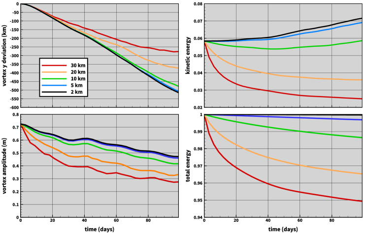
Figure 15: Time evolution of some revelant diagnostic quantities for the baroclinic vortex test case using the present second-order scheme. Simulations stabilization constants are $\gamma=0.2$ and $\alpha=0$ with the second-order scheme. Kinetic and total energies are computed from (46).

$\Delta x$	$\epsilon_{L_{2}}$	order		$\Delta x$	$\epsilon_{L_{2}}$	order
Vortex amplitude (m)				Vortex y-deviation (km)
$30\,\mathrm{\mathrm{km}}$	$1.99\>10^{-1}$	-		$30\,\mathrm{\mathrm{km}}$	$1.11\>10^{2}$	-
$20\,\mathrm{\mathrm{km}}$	$1.31\>10^{-1}$	$1.03$		$20\,\mathrm{\mathrm{km}}$	$6.37\>10^{1}$	$1.37$
$10\,\mathrm{\mathrm{km}}$	$4.37\>10^{-2}$	$1.58$		$10\,\mathrm{\mathrm{km}}$	$1.48\>10^{1}$	$2.11$
$5\,\mathrm{\mathrm{km}}$	$8.13\>10^{-3}$	$2.43$		$5\,\mathrm{km}$	$3.65\>10^{0}$	$2.02$
Kinetic Energy				Mechanical Energy
$30\,\mathrm{\mathrm{km}}$	$3.43\>10^{-2}$	-		$30\,\mathrm{\mathrm{km}}$	$4.07\>10^{-2}$	-
$20\,\mathrm{\mathrm{km}}$	$2.45\>10^{-2}$	$0.83$		$20\,\mathrm{\mathrm{km}}$	$2.63\>10^{-2}$	$1.08$
$10\,\mathrm{\mathrm{km}}$	$8.57\>10^{-3}$	$1.52$		$10\,\mathrm{\mathrm{km}}$	$8.80\>10^{-3}$	$1.58$
$5\,\mathrm{\mathrm{km}}$	$1.59\>10^{-3}$	$2.43$		$5\,\mathrm{\mathrm{km}}$	$1.70\>10^{-3}$	$2.37$

Table 3: Numerical convergence results for the baroclinic vortex using the present second-order scheme. The errors $\epsilon_{L^{2}}$ refer to the $L^{2}$ error norm in time between the numerical solution and the reference solution computed with $\Delta x=2\,\mathrm{km}$.

From a numerical stablity point of view, it can be observed for all the resolutions a strict decrease of the mechanical energy for the chosen pair of stabilization constants $\gamma$ and $\alpha$. It appears that the pressure stabilization term (12) is not required here to ensure a strict mechanical energy decrease, although the simulated flow is very complex. Since this term is proportional to the velocity divergence, it could be explained by a flow always very close to the incompressible condition. Another explanation could be the introduction of the Coriolis force that may have an impact on the stability conditions. We also performed another series of simulations for the $10\,\mathrm{km}$ resolution, with $\alpha=0.05\,,\,0.10\,,\,0.15$ and $0.20$ keeping the same other simulation parameters. The results given in Fig.16 show a quick deterioration for $\alpha$ increasing values. All the diagnostic quantities are approximately in the range of the $20\,\mathrm{\mathrm{km}}$ and $30\,\mathrm{\mathrm{km}}$ resolution results killing this stabilization term. The pressure term is impacted by a more important initial numerical imbalance. It can be easily verified looking at the initial kinetic energy decrease.

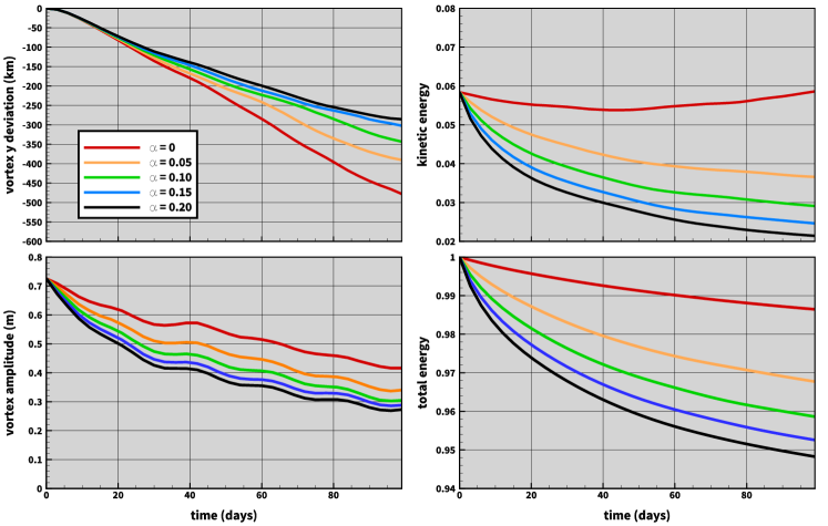
Figure 16: Time evolution of some revelant diagnostic quantities for the baroclinic vortex test case using the present second-order scheme. Simulations stabilization constants are $\gamma=0.2$ and some varying $\alpha$ with the second-order scheme and a fixed mesh size $\Delta x=10\,\mathrm{km}$.

6 Conclusion

In this paper we have introduced an explicit numerical scheme on unstructured meshes for the two-dimensional multilayer shallow water system with density stratification. The main characteristic of the numerical approach stands in its ability to deal with the non conservative pressure term with strong stability properties, and without the need of evaluating the system eigenvalues. The formalism is particularly adapted to deal with well-balancing issues, and a positivity result is also exhibited. Assuming a classical explicit CFL condition, the dissipation of the mechanical energy has been demonstrated under sufficient inequality conditions on a pair of stabilization constants, as well as the consistency with respect to the low Froude regimes at different time scales, which stand for two fundamental and challenging criteria in the context of large-scale oceanic or estuary flows. The non linear study has been complemented through a complete linear stability analysis for the the first and second-order schemes, for the one and two-dimensional problems. In particular, it has been observed that the calibration of the stabilization constants could be significantly relaxed at second-order with the use of an appropriate time scheme. The practical consequences are undeniable since it allows to considerably limit the diffusive losses in the numerical simulations. In view of these results, a more advanced high order space and time analysis is currently in progress, including an eventual extension to a general finite elements frame as we believe that the proposed numerical method gives a solid framework to derive high-order explicit schemes. As it is still confirmed by our numerical experiments, these stability properties make the approach particularly well suited to large-scale oceanic circulation, and competitive with other softwares developed within the oceanographic community.

In addition to high order space and time extensions, many other perspectives are driven by the present developments. First, the explicit scheme’s efficiency must be compared with its semi-implicit version [44], which accepts bigger time steps, but at the price of a more important computational cost (due to the resolution of a nonlinear system) and the difficulty to derive high order time and space extensions having the same strong stability properties. Thus, to date, the time benefits brought by the semi-implicit version are not so clear, especially since the use of bigger time steps tends to rapidly deteriorate the scheme’s accuracy. Appropriate high order schemes need to be used in order to limit this drawback. The global stability analysis of the numerical scheme taking into account the Coriolis force with or without time stepping also needs to be performed. In addition, and in view of very promising preliminary results, the present approach is currently oriented toward other crucial operational contexts such as river flows or coastal applications. These works need futher investigations to handle hydraulic jumps or wetting and drying areas, with the management of disappearing layers or emerging topographies. Also, in light of the numerical results, it appears crucial to study the possibility of computing the two adimensional stabilization constants locally, according notably to the discrete solution local regularity. This flexibility may substantially improve the overall accuracy of the method.

7 Appendix

The first part of this Appendix presents the main steps leading to the control of the total energy production (proof of Theorem 3.4). We then give an interpretation of the numerical model in terms convex combination of 1d schemes, as mentioned in Section 4. Some technical aspects for implementation purposes are also proposed, including the MUSCL reconstruction scheme (supplemented by a formal extension of energy dissipation results), treatment of Coriolis force and the fully explicit formula used for the time step selection.

7.1 Stability results for the first-order scheme

7.1.1 Kinetic energy

We begin by the kinetic energy, and set:

$${\mathcal{K}_{K,i}^{n}}=\frac{1}{2}{H_{K,i}^{n}}\left\|\textbf{u}_{K,i}^{n}\right\|^{2}\,.$$

We have the following result:

Proposition 7.1.

Estimation of the kinetic energy production

$${\mathcal{K}_{K,i}^{n+1}}-{\mathcal{K}_{K,i}^{n}}+\dfrac{\Delta t}{m_{K}}{\sum_{e\in\partial K}}\big{(}{\mathcal{G}_{\mathcal{K},e,i}^{n}}.{\textbf{n}_{e,K}}\big{)}{m_{e}}+\mathcal{Q}_{\mathcal{K},K,i}\leq\mathcal{R}_{\mathcal{K},K,i}+\mathcal{H}_{\mathcal{K},K,i}-\mathcal{A}_{\mathcal{K},K,i}+\tilde{\mathcal{A}}_{\mathcal{K},K,i}\,,$$

with

$${\mathcal{G}_{\mathcal{K},e,i}^{n}}.{\textbf{n}_{e,K}} =\frac{1}{2}\left\|\textbf{u}_{K,i}^{n}\right\|^{2}{\big{(}\mathcal{F}_{e,i}^{n}.\textbf{n}_{e,K}\big{)}^{+}}+\frac{1}{2}\left\|\textbf{u}_{K_{e},i}^{n}\right\|^{2}{\big{(}\mathcal{F}_{e,i}^{n}.\textbf{n}_{e,K}\big{)}^{-}}\,,$$

$$\mathcal{Q}_{\mathcal{K},K,i} =\dfrac{\Delta t}{m_{K}}{H_{K,i}^{n}}\textbf{u}_{K,i}^{n}.{\sum_{e\in\partial K}}\dfrac{{\boldsymbol{\delta}\Phi_{e,i}^{n}}}{\varepsilon^{2}}{m_{e}}\,,$$ (59)

$$\mathcal{H}_{\mathcal{K},K,i} =\dfrac{\Delta t}{m_{K}}{\sum_{e\in\partial K}}{\overline{H\textbf{u}}_{e,i}^{n}}.\dfrac{{\Lambda_{e,i}^{n}}}{\varepsilon^{2}}\textbf{n}_{e,K}{m_{e}}\,,$$

$$\mathcal{A}_{\mathcal{K},K,i} =\dfrac{\Delta t}{m_{K}}{\sum_{e\in\partial K}}\dfrac{{\Lambda_{e,i}^{n}}}{\varepsilon^{2}}\dfrac{1}{2}({H_{K_{e},i}^{n}}{\textbf{u}_{K_{e},i}^{n}}-{H_{K,i}^{n}}\textbf{u}_{K,i}^{n}).\textbf{n}_{e,K}{m_{e}}\,,$$ (60)

$$\tilde{\mathcal{A}}_{\mathcal{K},K,i} =2\left(\dfrac{\Delta t}{m_{K}}\right)^{2}\dfrac{({H_{K,i}^{n}})^{2}}{{H_{K,i}^{n+1}}}{m_{\partial K}}{\sum_{e\in\partial K}}\left(\dfrac{{\Lambda_{e,i}^{n}}}{\varepsilon^{2}}\right)^{2}{m_{e}}\,,$$ (61)

$$\mathcal{R}_{\mathcal{K},K,i} =\left(\dfrac{\Delta t}{m_{K}}\right)^{2}\dfrac{({H_{K,i}^{n}})^{2}}{{H_{K,i}^{n+1}}}{m_{\partial K}}{\sum_{e\in\partial K}}\left\|\dfrac{{\boldsymbol{\delta}\Phi_{e,i}^{n}}}{\varepsilon^{2}}\right\|^{2}{m_{e}}\,.$$ (62)

Proof.

We drop the subscript “i” for a better readability. We first use the equation on u (15):

$$\begin{split}{H_{K}^{n+1}}(\textbf{u}_{K}^{n+1}-\textbf{u}_{K}^{n}).\textbf{u}_{K}^{n}=&-\dfrac{\Delta t}{m_{K}}{\sum_{e\in\partial K}}({\textbf{u}_{K_{e}}^{n}}-\textbf{u}_{K}^{n}).\textbf{u}_{K}^{n}{\big{(}\mathcal{F}_{e}^{n}.\textbf{n}_{e,K}\big{)}^{-}}{m_{e}}\\ &-\dfrac{\Delta t}{m_{K}}{H_{K}^{n}}\textbf{u}_{K}^{n}.{\sum_{e\in\partial K}}\dfrac{{\Phi_{e}^{n,\ast}}}{\varepsilon^{2}}\textbf{n}_{e,K}{m_{e}}\,.\end{split}$$

Then, using the relation $(\textbf{a}-\textbf{b}).\textbf{b}=\dfrac{1}{2}\left\|\textbf{a}\right\|^{2}-\dfrac{1}{2}\left\|\textbf{b}\right\|^{2}-\dfrac{1}{2}\left\|\textbf{a}-\textbf{b}\right\|^{2}$ :

$$\begin{split}{H_{K}^{n+1}}\Big{(}\dfrac{1}{2}\left\|\textbf{u}_{K}^{n+1}\right\|^{2}&-\dfrac{1}{2}\left\|\textbf{u}_{K}^{n}\right\|^{2}-\dfrac{1}{2}\left\|\textbf{u}_{K}^{n+1}-\textbf{u}_{K}^{n}\right\|^{2}\Big{)}\\ =&-\dfrac{\Delta t}{m_{K}}{\sum_{e\in\partial K}}\Big{(}\dfrac{1}{2}\left\|\textbf{u}_{K_{e}}^{n}\right\|^{2}-\dfrac{1}{2}\left\|\textbf{u}_{K}^{n}\right\|^{2}-\dfrac{1}{2}\left\|{\textbf{u}_{K_{e}}^{n}}-\textbf{u}_{K}^{n}\right\|^{2}\Big{)}{\big{(}\mathcal{F}_{e}^{n}.\textbf{n}_{e,K}\big{)}^{-}}{m_{e}}\\ &-\dfrac{\Delta t}{m_{K}}{H_{K}^{n}}\textbf{u}_{K}^{n}.{\sum_{e\in\partial K}}\dfrac{{\Phi_{e}^{n,\ast}}}{\varepsilon^{2}}\textbf{n}_{e,K}{m_{e}}\,.\end{split}$$

previous equality and invoking the mass equation (9a), we have:

$$\begin{split}{\tilde{\mathcal{K}}_{K}^{n+1}}-{\tilde{\mathcal{K}}_{K}^{n}}=&-\dfrac{\Delta t}{m_{K}}{\sum_{e\in\partial K}}\Big{(}\frac{1}{2}\left\|\textbf{u}_{K}^{n}\right\|^{2}{\big{(}\mathcal{F}_{e}^{n}.\textbf{n}_{e,K}\big{)}^{+}}+\frac{1}{2}\left\|\textbf{u}_{K_{e}}^{n}\right\|^{2}{\big{(}\mathcal{F}_{e}^{n}.\textbf{n}_{e,K}\big{)}^{-}}\Big{)}{m_{e}}\\ &+\dfrac{1}{2}{H_{K}^{n+1}}\left\|\textbf{u}_{K}^{n+1}-\textbf{u}_{K}^{n}\right\|^{2}+\dfrac{\Delta t}{m_{K}}{\sum_{e\in\partial K}}\dfrac{1}{2}\left\|{\textbf{u}_{K_{e}}^{n}}-\textbf{u}_{K}^{n}\right\|^{2}{\big{(}\mathcal{F}_{e}^{n}.\textbf{n}_{e,K}\big{)}^{-}}{m_{e}}\\ &-\dfrac{\Delta t}{m_{K}}{H_{K}^{n}}\textbf{u}_{K}^{n}.{\sum_{e\in\partial K}}\dfrac{{\Phi_{e}^{n,\ast}}}{\varepsilon^{2}}\textbf{n}_{e,K}{m_{e}}\,.\end{split}$$ (63)

We now denote:

$$S_{K}=\dfrac{1}{2}{H_{K}^{n+1}}\left\|\textbf{u}_{K}^{n+1}-\textbf{u}_{K}^{n}\right\|^{2}+\dfrac{\Delta t}{m_{K}}{\sum_{e\in\partial K}}\dfrac{1}{2}\left\|{\textbf{u}_{K_{e}}^{n}}-\textbf{u}_{K}^{n}\right\|^{2}{\big{(}\mathcal{F}_{e}^{n}.\textbf{n}_{e,K}\big{)}^{-}}{m_{e}}\,,$$

focus on the first term of $S_{K}$. We first use Jensen’s inequality with the weights $1/4,1/2,1/4$ to obtain a control of the form:

$$\begin{split}\dfrac{1}{2}{H_{K}^{n+1}}\left\|\textbf{u}_{K}^{n+1}-\textbf{u}_{K}^{n}\right\|^{2}\leq&\quad\dfrac{\left({H_{K}^{n}}\right)^{2}}{{H_{K}^{n+1}}}\left(\dfrac{\Delta t}{m_{K}}\right)^{2}\left\|{\sum_{e\in\partial K}}\dfrac{{\boldsymbol{\delta}\Phi_{e}^{n}}}{\varepsilon^{2}}\textbf{n}_{e,K}{m_{e}}\right\|^{2}\\ &+2\dfrac{\left({H_{K}^{n}}\right)^{2}}{{H_{K}^{n+1}}}\left(\dfrac{\Delta t}{m_{K}}\right)^{2}\left\|{\sum_{e\in\partial K}}\dfrac{{\Lambda_{e}^{n}}}{\varepsilon^{2}}\textbf{n}_{e,K}{m_{e}}\right\|^{2}\\ &+\dfrac{2}{{H_{K}^{n+1}}}\left(\dfrac{\Delta t}{m_{K}}\right)^{2}\left\|{\sum_{e\in\partial K}}\left({\textbf{u}_{K_{e}}^{n}}-\textbf{u}_{K}^{n}\right){\big{(}\mathcal{F}_{e}^{n}.\textbf{n}_{e,K}\big{)}^{-}}{m_{e}}\right\|^{2}\,.\end{split}$$

We now carry on a separate analysis of each of the resulting terms. Using again Jensen’s inequality:

$$\begin{split}\left\|{\sum_{e\in\partial K}}\dfrac{{\overline{\Phi}_{e}^{n}}}{\varepsilon^{2}}\textbf{n}_{e,K}{m_{e}}\right\|^{2}&\leq{m_{\partial K}}\left({\sum_{e\in\partial K}}\left\|\dfrac{{\boldsymbol{\delta}\Phi_{e}^{n}}}{\varepsilon^{2}}\right\|^{2}{m_{e}}\right)\,,\\ \left\|{\sum_{e\in\partial K}}\dfrac{{\Lambda_{e}^{n}}}{\varepsilon^{2}}\textbf{n}_{e,K}{m_{e}}\right\|^{2}&\leq{m_{\partial K}}\left({\sum_{e\in\partial K}}\left(\dfrac{{\Lambda_{e}^{n}}}{\varepsilon^{2}}\right)^{2}{m_{e}}\right)\,.\end{split}$$ (64)

On the other hand, the Cauchy-Schwarz inequality gives:

$$\begin{split}\left\|{\sum_{e\in\partial K}}({\textbf{u}_{K_{e}}^{n}}-\textbf{u}_{K}^{n}){\big{(}\mathcal{F}_{e}^{n}.\textbf{n}_{e,K}\big{)}^{-}}{m_{e}}\right\|^{2}\leq&\Big{(}{\sum_{e\in\partial K}}\left\|{\textbf{u}_{K_{e}}^{n}}-\textbf{u}_{K}^{n}\right\|^{2}{\big{(}\mathcal{F}_{e}^{n}.\textbf{n}_{e,K}\big{)}^{-}}{m_{e}}\Big{)}\Big{(}{\sum_{e\in\partial K}}{\big{(}\mathcal{F}_{e}^{n}.\textbf{n}_{e,K}\big{)}^{-}}{m_{e}}\Big{)}\,.\end{split}$$

Thus:

$$\begin{split}S_{K}\leq&\left(\dfrac{\Delta t}{m_{K}}\right)^{2}\dfrac{({H_{K}^{n}})^{2}}{{H_{K}^{n+1}}}{m_{\partial K}}\left({\sum_{e\in\partial K}}\left\|\dfrac{{\boldsymbol{\delta}\Phi_{e}^{n}}}{\varepsilon^{2}}\right\|^{2}{m_{e}}\right)+2\left(\dfrac{\Delta t}{m_{K}}\right)^{2}\dfrac{({H_{K}^{n}})^{2}}{{H_{K}^{n+1}}}{m_{\partial K}}\left({\sum_{e\in\partial K}}\left(\dfrac{{\Lambda_{e}^{n}}}{\varepsilon^{2}}\right)^{2}{m_{e}}\right)\\ +&\dfrac{1}{2}\dfrac{\Delta t}{m_{K}}{\sum_{e\in\partial K}}\left\|{\textbf{u}_{K_{e}}^{n}}-\textbf{u}_{K}^{n}\right\|^{2}{\big{(}\mathcal{F}_{e}^{n}.\textbf{n}_{e,K}\big{)}^{-}}{m_{e}}\times\Big{[}1-4\dfrac{\Delta t}{m_{K}}{\sum_{e\in\partial K}}\frac{-{\big{(}\mathcal{F}_{e}^{n}.\textbf{n}_{e,K}\big{)}^{-}}}{{H_{K}^{n+1}}}{m_{e}}\Big{]}\,.\end{split}$$ (65)

The third term being assumed negative according to Remark 3.3 (condition (23) with $\beta=1/4$), this yields the remainder $\mathcal{R}_{\mathcal{K},K,i}$ (62) and the contribution $\tilde{\mathcal{A}}_{\mathcal{K},K,i}$ (61). Finally, using again (16) the term involving the potential forces in (63) is rewritten as:

$$\begin{split}\dfrac{\Delta t}{m_{K}}{H_{K}^{n}}\textbf{u}_{K}^{n}.{\sum_{e\in\partial K}}\dfrac{{\Phi_{e}^{n,\ast}}}{\varepsilon^{2}}\textbf{n}_{e,K}{m_{e}}&=\dfrac{\Delta t}{m_{K}}{H_{K}^{n}}\textbf{u}_{K}^{n}.{\sum_{e\in\partial K}}\dfrac{{\boldsymbol{\delta}\Phi_{e}^{n}}}{\varepsilon^{2}}{m_{e}}-\dfrac{\Delta t}{m_{K}}{H_{K}^{n}}\textbf{u}_{K}^{n}.{\sum_{e\in\partial K}}\dfrac{{\Lambda_{e}^{n}}}{\varepsilon^{2}}\textbf{n}_{e,K}{m_{e}}\,.\end{split}$$

We use the relation ${H_{K}^{n}}\textbf{u}_{K}^{n}={\overline{H\textbf{u}}_{e}^{n}}+\dfrac{1}{2}({H_{K}^{n}}\textbf{u}_{K}^{n}-{H_{K_{e}}^{n}}{\textbf{u}_{K_{e}}^{n}})$ on the second member of the right hand side in the previous equality, to finally obtain $\mathcal{Q}_{\mathcal{K},K,i}$, $\mathcal{H}_{\mathcal{K},K,i}$ and $\mathcal{A}_{\mathcal{K},K,i}$.∎

7.1.2 Potential energy

We now turn to the potential part, and denote ${\mathcal{E}_{K}^{n}}$ the potential energy on the cell $K$ at time $n$. We have the following result:

Proposition 7.2.

Estimation of the potential energy production:

$${\mathcal{E}_{K}^{n+1}}-{\mathcal{E}_{K}^{n}}+\dfrac{\Delta t}{m_{K}}{\sum_{i=1}^{L}}{\sum_{e\in\partial K}}\big{(}{\mathcal{G}_{\mathcal{E},e,i}^{n}}.{\textbf{n}_{e,K}}\big{)}{m_{e}}-\mathcal{Q}_{\mathcal{E},K}\leq-\mathcal{R}_{\mathcal{E},K}+\mathcal{H}_{\mathcal{E},K}+\mathcal{A}_{\mathcal{E},K}+\tilde{\mathcal{R}}_{\mathcal{E},K}\,,$$

with

$${\mathcal{G}_{\mathcal{E},e,i}^{n}}.{\textbf{n}_{e,K}} ={\overline{\Phi}_{e,i}^{n}}\mathcal{F}_{e,i}^{n}.\textbf{n}_{e,K}\,,$$

$$\mathcal{Q}_{\mathcal{E},K} =\dfrac{\Delta t}{m_{K}}{\sum_{i=1}^{L}}{H_{K,i}^{n}}\textbf{u}_{K,i}^{n}.{\sum_{e\in\partial K}}{\boldsymbol{\delta}\Phi_{e,i}^{n}}{m_{e}}\,,$$ (66)

$$\mathcal{R}_{\mathcal{E},K} =\dfrac{\Delta t}{m_{K}}{\sum_{i=1}^{L}}{\sum_{e\in\partial K}}\Pi_{e,i}^{n}.{\boldsymbol{\delta}\Phi_{e,i}^{n}}{m_{e}}\,,$$ (67)

$$\mathcal{H}_{\mathcal{E},K} =\dfrac{\Delta t}{m_{K}}{\sum_{i=1}^{L}}{\sum_{e\in\partial K}}\left(\dfrac{{H_{K_{e},i}^{n}}{\textbf{u}_{K_{e},i}^{n}}-{H_{K,i}^{n}}\textbf{u}_{K,i}^{n}}{2}\right).{\boldsymbol{\delta}\Phi_{e,i}^{n}}{m_{e}}\,,$$

and the Taylor’s residuals:

$$\tilde{\mathcal{R}}_{\mathcal{E},K} ={C_{{\boldsymbol{\mathcal{H}}}}}\left(\dfrac{\Delta t}{m_{K}}\right)^{2}{m_{\partial K}}{\sum_{i=1}^{L}}{\sum_{e\in\partial K}}(\Pi_{e,i}^{n}.\textbf{n}_{e,K})^{2}{m_{e}}\,,$$ (68)

$$\mathcal{A}_{\mathcal{E},K} ={C_{{\boldsymbol{\mathcal{H}}}}}\left(\dfrac{\Delta t}{m_{K}}\right)^{2}{m_{\partial K}}{\sum_{i=1}^{L}}{\sum_{e\in\partial K}}({{\delta}(H\textbf{u})_{e,i}^{n}})^{2}{m_{e}}\,.$$ (69)

Proof.

Using Taylor’s formula between time steps $n$ and $n+1$, we have for a certain $s\in\left[0,1\right]$:

$${\mathcal{E}_{K}^{n+1}}-{\mathcal{E}_{K}^{n}}=-\dfrac{\Delta t}{m_{K}}{\sum_{i=1}^{L}}{\sum_{e\in\partial K}}{\Phi_{K,i}^{n}}\mathcal{F}_{e,i}^{n}.\textbf{n}_{e,K}{m_{e}}+\dfrac{1}{2}{\sum_{i=1}^{L}}{\sum_{j=1}^{L}}\big{(}{H_{K,i}^{n+1}}-{H_{K,i}^{n}}\big{)}{\boldsymbol{\mathcal{H}}}_{ij,K}^{n+s}\big{(}H_{K,j}^{n+1}-H_{K,j}^{n}\big{)}\,,$$

where ${\boldsymbol{\mathcal{H}}}_{ij,K}^{n+s}={\boldsymbol{\mathcal{H}}}_{ij}\left(s{\boldsymbol{H}}_{K}^{n+1}+(1-s){\boldsymbol{H}}_{K}^{n},\mathbf{x}_{K}\right)$, where we recall that $\boldsymbol{{\boldsymbol{H}}}_{K}^{n}=\leftidx{{}^{t}}{\left(H_{K,1}^{n},\cdots,H_{K,L}^{n}\right)}$. Then we call the following decomposition:

$$\begin{split}{\Phi_{K,i}^{n}}\mathcal{F}_{e,i}^{n}.\textbf{n}_{e,K}{m_{e}}&={\overline{\Phi}_{e,i}^{n}}\mathcal{F}_{e,i}^{n}.\textbf{n}_{e,K}{m_{e}}+({\Phi_{K,i}^{n}}-{\overline{\Phi}_{e,i}^{n}})\mathcal{F}_{e,i}^{n}.\textbf{n}_{e,K}{m_{e}}\\ &={\overline{\Phi}_{e,i}^{n}}\mathcal{F}_{e,i}^{n}.\textbf{n}_{e,K}{m_{e}}-{\overline{H\textbf{u}}_{e,i}^{n}}.\boldsymbol{\delta}\Phi_{e,i}^{n}{m_{e}}+\Pi_{e,i}^{n}.\boldsymbol{\delta}\Phi_{e,i}^{n}{m_{e}}\,.\end{split}$$

Expanding ${\overline{H\textbf{u}}_{e,i}^{n}}={H_{K,i}^{n}}\textbf{u}_{K,i}^{n}+\left(\dfrac{{H_{K_{e},i}^{n}}{\textbf{u}_{K_{e},i}^{n}}-{H_{K,i}^{n}}\textbf{u}_{K,i}^{n}}{2}\right)$ we recover the symmetric fluxes ${\mathcal{G}_{\mathcal{E},e,i}^{n}}.{\textbf{n}_{e,K}}$ and the residuals $\mathcal{Q}_{\mathcal{E},K}$, $\mathcal{R}_{\mathcal{E},K}$, $\mathcal{H}_{\mathcal{E},K}$. Concerning now the Taylor’s residual, we have, according to (7):

$$\mathcal{W}_{\mathcal{E},K}:=\dfrac{1}{2}{\sum_{i=1}^{L}}{\sum_{j=1}^{L}}\big{(}{H_{K,i}^{n+1}}-{H_{K,i}^{n}}\big{)}{\boldsymbol{\mathcal{H}}}_{ij,K}^{n+s}\big{(}H_{K,j}^{n+1}-H_{K,j}^{n}\big{)}\leq\dfrac{1}{2}{C_{{\boldsymbol{\mathcal{H}}}}}{\sum_{i=1}^{L}}\left({H_{K,i}^{n+1}}-{H_{K,i}^{n}}\right)^{2}\,.$$ (70)

We then reformulate (9a):

$$\begin{split}{H_{K,i}^{n+1}}-{H_{K,i}^{n}}&=-\dfrac{\Delta t}{m_{K}}{\sum_{e\in\partial K}}\mathcal{F}_{e,i}^{n}.\textbf{n}_{e,K}{m_{e}}=-\dfrac{\Delta t}{m_{K}}{\sum_{e\in\partial K}}{\overline{H\textbf{u}}_{e,i}^{n}}.\textbf{n}_{e,K}{m_{e}}+\dfrac{\Delta t}{m_{K}}{\sum_{e\in\partial K}}\Pi_{e,i}^{n}.\textbf{n}_{e,K}{m_{e}}\,,\\ &=-\dfrac{\Delta t}{m_{K}}{\sum_{e\in\partial K}}{{\delta}(H\textbf{u})_{e,i}^{n}}{m_{e}}+\dfrac{\Delta t}{m_{K}}{\sum_{e\in\partial K}}\Pi_{e,i}^{n}.\textbf{n}_{e,K}{m_{e}}\,,\end{split}$$

where we recall that ${{\delta}(H\textbf{u})_{e,i}^{n}}=\dfrac{1}{2}({H_{K_{e},i}^{n}}{\textbf{u}_{K_{e},i}^{n}}-{H_{K,i}^{n}}\textbf{u}_{K,i}^{n}).\textbf{n}_{e,K}$. Injecting this in (70), we use Jensen’s inequality to obtain:

$$\begin{split}\mathcal{W}_{\mathcal{E},K}\leq&{C_{{\boldsymbol{\mathcal{H}}}}}{\sum_{i=1}^{L}}\left(\dfrac{\Delta t}{m_{K}}{\sum_{e\in\partial K}}{{\delta}(H\textbf{u})_{e,i}^{n}}{m_{e}}\right)^{2}+{C_{{\boldsymbol{\mathcal{H}}}}}{\sum_{i=1}^{L}}\left(\dfrac{\Delta t}{m_{K}}{\sum_{e\in\partial K}}\Pi_{e,i}^{n}.\textbf{n}_{e,K}{m_{e}}\right)^{2}\\ \leq&{C_{{\boldsymbol{\mathcal{H}}}}}\left(\dfrac{\Delta t}{m_{K}}\right)^{2}{m_{\partial K}}{\sum_{i=1}^{L}}{\sum_{e\in\partial K}}({{\delta}(H\textbf{u})_{e,i}^{n}})^{2}{m_{e}}+{C_{{\boldsymbol{\mathcal{H}}}}}\left(\dfrac{\Delta t}{m_{K}}\right)^{2}{m_{\partial K}}{\sum_{i=1}^{L}}{\sum_{e\in\partial K}}(\Pi_{e,i}^{n}.\textbf{n}_{e,K})^{2}{m_{e}}\,,\end{split}$$ (71)

and fall on the two remaining terms of the estimation.∎

7.1.3 Total energy

Let’s now consider ${E^{n}}={\displaystyle\sum_{K\in\mathbb{T}}{m_{K}}\left({\mathcal{E}_{K}^{n}}/\varepsilon^{2}+{\displaystyle{\sum_{i=1}^{L}}{\mathcal{K}_{K,i}^{n}}}\right)}$ the discrete mechanical energy, and focus on the non-antisymmetric terms. We first observe an exact balance between the terms (59) and (66) arising from the kinetic and potential parts. In consequence the effort is put on a simultaneous control of the terms $\mathcal{R}$ and $\mathcal{A}$ appearing in the kinetic and potential energy budgets.

Estimate 1 :

We gather the contributions issuing from the estimations on the kinetic and potential discrete energies, i.e. (62) and (67, 68) respectively:

$$\begin{split}{m_{K}}{\sum_{i=1}^{L}}\mathcal{R}_{\mathcal{K},K,i}&=\left(\Delta t\right)^{2}{\sum_{i=1}^{L}}\left(\dfrac{({H_{K,i}^{n}})^{2}}{{H_{K,i}^{n+1}}}\dfrac{{m_{\partial K}}}{{m_{K}}}\right){\sum_{e\in\partial K}}\left\|\dfrac{{\boldsymbol{\delta}\Phi_{e,i}^{n}}}{\varepsilon^{2}}\right\|^{2}{m_{e}}\,,\\ -{m_{K}}\mathcal{R}_{\mathcal{E},K}/\varepsilon^{2}&=-\Delta t{\sum_{i=1}^{L}}{\sum_{e\in\partial K}}\Pi_{e,i}^{n}.\dfrac{{\boldsymbol{\delta}\Phi_{e,i}^{n}}}{\varepsilon^{2}}{m_{e}}\,,\\ {m_{K}}\tilde{\mathcal{R}}_{\mathcal{E},K}/\varepsilon^{2}&=\left(\Delta t\right)^{2}{C_{{\boldsymbol{\mathcal{H}}}}}\left(\dfrac{{m_{\partial K}}}{{m_{K}}}\right){\sum_{i=1}^{L}}{\sum_{e\in\partial K}}\left(\dfrac{\Pi_{e,i}^{n}.\textbf{n}_{e,K}}{\varepsilon}\right)^{2}{m_{e}}\,.\end{split}$$

As a preliminary step, we define:

$$\widehat{H}_{K,i}^{n}:=\dfrac{({H_{K,i}^{n}})^{2}}{{H_{K,i}^{n+1}}}=H_{K,i}^{n}+\mathcal{O}(\Delta t)\,.$$ (72)

Then, using $\left(\dfrac{({H_{K,i}^{n}})^{2}}{{H_{K,i}^{n+1}}}\dfrac{{m_{\partial K}}}{{m_{K}}}\right)=2\left(\dfrac{\widehat{H}}{{\Delta}}\right)_{K,i}^{n}=\left(\left(\dfrac{\widehat{H}}{{\Delta}}\right)_{K,i}^{n}+\left(\dfrac{\widehat{H}}{{\Delta}}\right)_{K_{e},i}^{n}\right)+\left(\left(\dfrac{\widehat{H}}{{\Delta}}\right)_{K,i}^{n}-\left(\dfrac{\widehat{H}}{{\Delta}}\right)_{K_{e},i}^{n}\right)$, we split the first contribution ${m_{K}}{\sum_{i=1}^{L}}\mathcal{R}_{\mathcal{K},K,i}$ in a sum of symmetric and antisymmetric parts:

$$\begin{split}{m_{K}}{\sum_{i=1}^{L}}\mathcal{R}_{\mathcal{K},K,i}&=\left(\Delta t\right)^{2}{\sum_{i=1}^{L}}{\sum_{e\in\partial K}}2\left(\dfrac{\widehat{H}}{{\Delta}}\right)_{e,i}^{n}\left\|\dfrac{{\boldsymbol{\delta}\Phi_{e,i}^{n}}}{\varepsilon^{2}}\right\|^{2}{m_{e}}\,\\ &+\left(\Delta t\right)^{2}{\sum_{i=1}^{L}}{\sum_{e\in\partial K}}\frac{1}{2}\left(\left(\dfrac{\widehat{H}}{{\Delta}}\right)_{K,i}^{n}-\left(\dfrac{\widehat{H}}{{\Delta}}\right)_{K_{e},i}^{n}\right)\left\|\dfrac{{\boldsymbol{\delta}\Phi_{e,i}^{n}}}{\varepsilon^{2}}\right\|^{2}{m_{e}}\,.\end{split}$$

In a similar way, with $\dfrac{1}{\Delta_{K}}=\dfrac{1}{2}\left(\dfrac{1}{\Delta_{K}}+\dfrac{1}{\Delta_{K_{e}}}\right)+\dfrac{1}{2}\left(\dfrac{1}{\Delta_{K}}-\dfrac{1}{\Delta_{K_{e}}}\right)$, the term ${m_{K}}\tilde{\mathcal{R}}_{\mathcal{E},K}/\varepsilon^{2}$ reads:

$$\begin{split}{m_{K}}\tilde{\mathcal{R}}_{\mathcal{E},K}/\varepsilon^{2}&=\left(\Delta t\right)^{2}{\sum_{i=1}^{L}}{\sum_{e\in\partial K}}\frac{{C_{{\boldsymbol{\mathcal{H}}}}}}{\Delta_{e}}\left(\dfrac{\Pi_{e,i}^{n}.\textbf{n}_{e,K}}{\varepsilon}\right)^{2}{m_{e}}\,\\ &+\left(\Delta t\right)^{2}{\sum_{i=1}^{L}}{\sum_{e\in\partial K}}\frac{{C_{{\boldsymbol{\mathcal{H}}}}}}{2}\left(\frac{1}{\Delta_{K}}-\frac{1}{\Delta_{K_{e}}}\right)\left(\dfrac{\Pi_{e,i}^{n}.\textbf{n}_{e,K}}{\varepsilon}\right)^{2}{m_{e}}\,.\end{split}$$

Dropping the antisymmetric terms, which vanish after global summation, we use (12):

$$\Pi_{e,i}^{n}=\gamma\Delta t\left(\dfrac{\widehat{H}}{{\Delta}}\right)_{e,i}^{n}\dfrac{{\boldsymbol{\delta}\Phi_{e,i}^{n}}}{\varepsilon^{2}}\,\,\,,\,\,\gamma>0\,,$$

to write the total contribution as:

$$\begin{split}\sum_{K\in\mathbb{T}}{m_{K}}\left({\sum_{i=1}^{L}}\mathcal{R}_{\mathcal{K},K,i}\tilde{\mathcal{R}}_{\mathcal{E},K}/\varepsilon^{2}-\mathcal{R}_{\mathcal{E},K}/\varepsilon^{2}+\tilde{\mathcal{R}}_{\mathcal{E},K}/\varepsilon^{2}\right)\qquad\qquad\qquad\\ =\left(\Delta t\right)^{2}\sum_{K\in\mathbb{T}}{\sum_{i=1}^{L}}{\sum_{e\in\partial K}}\left[2+\gamma^{2}\left(\dfrac{\left(\Delta t\right)^{2}}{\varepsilon^{2}}\frac{{C_{{\boldsymbol{\mathcal{H}}}}}}{\Delta_{e}}\left(\dfrac{\widehat{H}}{{\Delta}}\right)_{e,i}^{n}\right)-\gamma\right]&\left(\dfrac{\widehat{H}}{{\Delta}}\right)_{e,i}^{n}\left\|\dfrac{{\boldsymbol{\delta}\Phi_{e,i}^{n}}}{\varepsilon^{2}}\right\|^{2}{m_{e}}\,.\end{split}$$ (73)

Defining the quantity $\rho_{\varepsilon}$ such that:

$$\rho_{\varepsilon}^{2}=2\dfrac{\left(\Delta t\right)^{2}}{\varepsilon^{2}}\frac{{C_{{\boldsymbol{\mathcal{H}}}}}}{\Delta_{e}}\left(\dfrac{\widehat{H}}{{\Delta}}\right)_{e,i}^{n}\,,$$ (74)

the negativity of (73) reduces to:

$$p(\gamma)=\frac{1}{2}\rho_{\varepsilon}^{2}\gamma^{2}-\gamma+2\leq 0\,.$$ (75)

Based on the positivity of the discriminant (that is $\rho_{\varepsilon}\leq\dfrac{1}{2}$) and the roots of $p$: $\gamma^{\pm}=\dfrac{1\pm\sqrt{1-4\rho_{\varepsilon}^{2}}}{\rho_{\varepsilon}^{2}}$, one can establish that the value $\gamma=4$ ensures the negativity of $p$.

Estimate 2:

We consider the three remaining terms involved in the energy budget (60), (61) and (69):

$$\begin{split}-{m_{K}}{\sum_{i=1}^{L}}\mathcal{A}_{\mathcal{K},K,i}&=-\Delta t{\sum_{i=1}^{L}}{\sum_{e\in\partial K}}\dfrac{{\Lambda_{e,i}^{n}}}{\varepsilon^{2}}{{\delta}(H\textbf{u})_{e,i}^{n}}{m_{e}}\,,\\ {m_{K}}{\sum_{i=1}^{L}}\tilde{\mathcal{A}}_{\mathcal{K},K,i}&=2\left(\Delta t\right)^{2}{\sum_{i=1}^{L}}\left(\dfrac{({H_{K,i}^{n}})^{2}}{{H_{K,i}^{n+1}}}\dfrac{{m_{\partial K}}}{{m_{K}}}\right){\sum_{e\in\partial K}}\left(\dfrac{{\Lambda_{e,i}^{n}}}{\varepsilon^{2}}\right)^{2}{m_{e}}\,,\\ {m_{K}}\mathcal{A}_{\mathcal{E},K}/\varepsilon^{2}&=\left(\Delta t\right)^{2}{C_{{\boldsymbol{\mathcal{H}}}}}\left(\dfrac{{m_{\partial K}}}{{m_{K}}}\right){\sum_{i=1}^{L}}{\sum_{e\in\partial K}}({{\delta}(H\textbf{u})_{e,i}^{n}}/\varepsilon)^{2}{m_{e}}\,.\end{split}$$

In the spirit of the previous analysis we decompose ${m_{K}}{\sum_{i=1}^{L}}\tilde{\mathcal{A}}_{\mathcal{K},K,i}$ and ${m_{K}}{\sum_{i=1}^{L}}\mathcal{A}_{\mathcal{E},K}$ as follows:

$$\begin{split}{m_{K}}{\sum_{i=1}^{L}}\tilde{\mathcal{A}}_{\mathcal{K},K,i}&=4\left(\Delta t\right)^{2}{\sum_{i=1}^{L}}{\sum_{e\in\partial K}}\left(\dfrac{\widehat{H}}{{\Delta}}\right)_{e,i}^{n}\left(\dfrac{{\Lambda_{e,i}^{n}}}{\varepsilon^{2}}\right)^{2}{m_{e}}\,\\ &+\left(\Delta t\right)^{2}{\sum_{i=1}^{L}}{\sum_{e\in\partial K}}\left(\left(\dfrac{\widehat{H}}{{\Delta}}\right)_{K,i}^{n}-\left(\dfrac{\widehat{H}}{{\Delta}}\right)_{K_{e},i}^{n}\right)\left(\dfrac{{\Lambda_{e,i}^{n}}}{\varepsilon^{2}}\right)^{2}{m_{e}}\,\\ {m_{K}}\mathcal{A}_{\mathcal{E},K}/\varepsilon^{2}&=\left(\Delta t\right)^{2}{\sum_{i=1}^{L}}{\sum_{e\in\partial K}}\frac{{C_{{\boldsymbol{\mathcal{H}}}}}}{\Delta_{e}}({{\delta}(H\textbf{u})_{e,i}^{n}}/\varepsilon)^{2}{m_{e}}\,\\ &+\left(\Delta t\right)^{2}{\sum_{i=1}^{L}}{\sum_{e\in\partial K}}\frac{{C_{{\boldsymbol{\mathcal{H}}}}}}{2}\left(\frac{1}{\Delta_{K}}-\frac{1}{\Delta_{K_{e}}}\right)({{\delta}(H\textbf{u})_{e,i}^{n}}/\varepsilon)^{2}{m_{e}}\,.\end{split}$$

Again we neglect the antisymmetric terms, and consider (12):

$${\Lambda_{e,i}^{n}}=\alpha{C_{{\boldsymbol{\mathcal{H}}}}}\Delta t\frac{{{\delta}(H\textbf{u})_{e,i}^{n}}}{\Delta_{e}}\quad,\quad\alpha>0\,.$$

The total contribution attached to these terms becomes:

$$\begin{split}\sum_{K\in\mathbb{T}}{\sum_{e\in\partial K}}{m_{K}}\left(-{\sum_{i=1}^{L}}\tilde{\mathcal{A}}_{\mathcal{K},K,i}+{\sum_{i=1}^{L}}\tilde{\mathcal{A}}_{\mathcal{K},K,i}+\mathcal{A}_{\mathcal{E},K}/\varepsilon^{2}\right)\qquad\qquad\\ =\left(\Delta t\right)^{2}\sum_{K\in\mathbb{T}}{\sum_{i=1}^{L}}{\sum_{e\in\partial K}}\left[-\alpha+\alpha^{2}\left(4\dfrac{\left(\Delta t\right)^{2}}{\varepsilon^{2}}\frac{{C_{{\boldsymbol{\mathcal{H}}}}}}{\Delta_{e}}\left(\dfrac{\widehat{H}}{{\Delta}}\right)_{e,i}^{n}\right)+1\right]&\frac{{C_{{\boldsymbol{\mathcal{H}}}}}}{\Delta_{e}}\left(\dfrac{{{\delta}(H\textbf{u})_{e,i}^{n}}}{\varepsilon}\right)^{2}{m_{e}}\,.\end{split}$$ (76)

Using the same notations as previously, we are this time left with the study of the second-order polynomial:

$$q(\alpha)=2\rho_{\varepsilon}^{2}\alpha^{2}-\alpha+1\leq 0\,.$$ (77)

Supposing that $\rho_{\varepsilon}\leq\dfrac{1}{2\sqrt{2}}$, the real roots are $\alpha^{\pm}=\dfrac{1\pm\sqrt{1-8\rho_{\varepsilon}^{2}}}{4\rho_{\varepsilon}^{2}}$, from which we extract the value $\alpha=2$.

7.2 Reformulation as convex combination of 1d schemes

Following the ideas of [9] (see also [26] for an application to the Shallow Water equations), each cell $K$ is divided in a subgrid made of triangles $T_{K,e}$, connecting the edges $e\in\partial K$ to the mass center of $K$ (see Fig.17).

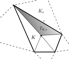
Figure 17: Mesh subgrid associated with an element $K$. Focus on the interface $e$: the triangle $T_{K,e}$ connects $e$ to the mass center of $K$.

Gathering the discrete variables of the model in the vectors ${\mathbf{W}}_{K}$, the mass and momentum fluxes involved in the scheme (9a, 9b), together with the discrete gradient pressure, can be reformulated in terms of functions of ${\mathbf{W}}_{K},\,{\mathbf{W}}_{K_{e}}$ and $n_{e,K}$ , through the following notations (we drop the subscript “i” to alleviate the notations):

$$\mathcal{F}_{e}^{n}.\mathbf{n}_{e,K} =\mathcal{F}({\mathbf{W}}_{K}^{n},\,{\mathbf{W}}_{K_{e}}^{n},\,{\mathbf{n}}_{e,K})$$

$$\mathcal{G}_{e}^{n}.\mathbf{n}_{e,K} =\mathcal{G}({\mathbf{W}}_{K}^{n},\,{\mathbf{W}}_{K_{e}}^{n},\,{\mathbf{n}}_{e,K})=\mathbf{u}_{K}^{n}\left(\mathcal{F}_{e}^{n}.\mathbf{n}_{e,K}\right)^{+}+\mathbf{u}_{K_{e}}^{n}\left(\mathcal{F}_{e}^{n}.\mathbf{n}_{e,K_{e}}\right)^{-}\qquad.$$ (78)

$$\mathcal{P}_{e}^{n} ={\Phi_{e}^{n,\ast}}{\mathbf{n}}_{e,K}=\mathcal{P}({\mathbf{W}}_{K}^{n},\,{\mathbf{W}}_{K_{e}}^{n},\,{\mathbf{n}}_{e,K})\,$$

Then, denoting $m_{T_{K,e}}$ the area of $T_{K,e}$, the scheme (9a, 9b) can be written as a convex combination of one-dimensional schemes:

$$H_{K}^{n+1} ={\displaystyle\sum_{e\in\partial K}\dfrac{m_{T_{K,e}}}{m_{K}}H_{e}^{n+1}}$$ (79a)

$$H_{K}^{n+1}\mathbf{u}_{K}^{n+1} ={\displaystyle\sum_{e\in\partial K}\dfrac{m_{T_{K,e}}}{m_{K}}H_{e}^{n+1}\mathbf{u}_{e}^{n+1}}\,$$ (79b)

where we have introduced the auxiliary variables:

$$H_{e}^{n+1} =H_{K}^{n}-{\displaystyle\dfrac{\Delta t}{\Delta x_{e}}\left[\mathcal{F}({\mathbf{W}}_{K},\,{\mathbf{W}}_{K_{e}},\,{\mathbf{n}}_{e,K})-\mathcal{F}({\mathbf{W}}_{K},\,{\mathbf{W}}_{K},\,{\mathbf{n}}_{e,K})\right]}$$ (80a)

$$H_{e}^{n+1}\mathbf{u}_{e}^{n+1} =H_{K}^{n}\mathbf{u}_{K}^{n}-{\displaystyle\dfrac{\Delta t}{\Delta x_{e}}\left[\mathcal{G}({\mathbf{W}}_{K},\,{\mathbf{W}}_{K_{e}},\,{\mathbf{n}}_{e,K})-\mathcal{G}({\mathbf{W}}_{K},\,{\mathbf{W}}_{K},\,{\mathbf{n}}_{e,K})\right]}$$ (80b)

$$\qquad\qquad-{\displaystyle\dfrac{\Delta t}{\Delta x_{e}}H_{K}^{n}\left[\mathcal{P}({\mathbf{W}}_{K},\,{\mathbf{W}}_{K_{e}},\,{\mathbf{n}}_{e,K})-\mathcal{P}({\mathbf{W}}_{K},\,{\mathbf{W}}_{K},\,{\mathbf{n}}_{e,K})\right]}\,$$

and the geometric constant $\Delta x_{e}=\dfrac{m_{T_{K,e}}}{m_{e}}$.

7.3 Second-order extension

7.3.1 MUSCL reconstructions

We consider in this work a monoslope second-order MUSCL scheme, which consists of local linear reconstructions by computing a vectorial slope $\left[\mathbf{\nabla}\mathbf{W}_{K}\right]_{m}$ in each cell $K$ and for each primitive variable $m$, such that the two reconstructed primitive variables vectors $\mathbf{W}_{e,K}$ and $\mathbf{W}_{e,K_{e}}$ are evaluated at each side of edge $e$ by:

$$\begin{array}[]{c}\mathbf{W}_{e,K_{\phantom{e}}}=\mathbf{W}_{K_{\phantom{e}}}+\mathbf{\nabla}\mathbf{W}_{K_{\phantom{e}}}.\mathbf{x}_{K_{\phantom{e}}}\mathbf{x}_{e}\\ \mathbf{W}_{e,K_{e}}=\mathbf{W}_{K_{e}}+\mathbf{\nabla}\mathbf{W}_{K_{e}}.\mathbf{x}_{K_{e}}\mathbf{x}_{e}\end{array}\,.$$ (81)

These quantities are intended to replace the primitive variables in the first-order scheme (Eqs.9a-9b-10b-10a) to evaluate the numerical flux $\mathcal{F}_{e}^{n}$ and the pressure $\Phi_{e}^{n,\ast}$ at the edge $e$. Classically, with such a linear reconstruction, one can expect a scheme with a second-order accuracy in space for sufficient regular solutions. To this end, a least square method is employed to compute the vectorial slopes for each primitive variable $h_{K}^{n}$, $u_{K}^{n}$ and $v_{K}^{n}$. More explicitly, the following sums of squares

$$\begin{array}[]{c}E_{m}\left(\left[\mathbf{\nabla}\mathbf{W}_{K}\right]_{m}\right)={\displaystyle\sum_{e\in\partial K}\left(\left[\mathbf{W}_{K_{e}}\right]_{m}-\left(\left[\mathbf{W}_{K}\right]_{m}+\left[\mathbf{\nabla}\mathbf{W}_{K}\right]_{m}.\mathbf{x}_{K}\mathbf{x}_{K_{e}}\right)\right)^{2}}\end{array}\,,$$ (82)

are minimized by setting the gradients to zero solution of simple 2 x 2 linear systems. This method represents a good alternative among others to find the hyperplane because of its accuracy and robustness, independently from the number of neighbours. No limitation is imposed to the computed vectorial slope because most of the numerical solutions considered in this work are largely sufficiently regular and far from wet/dry conditions to ensure numerical stability (except a Barth limiter [7] for the lake test case §5.3).

7.3.2 Second-order scheme

With the two reconstructed primitive variables vectors $\mathbf{W}_{e,K}^{n}$ and $\mathbf{W}_{e,K_{e}}^{n}$ at each side of the edge $e$, interface terms are simply replaced in the original first-order scheme. In the general $L$ layer case, and omitting the subscript “i” referring to the layer numbering for the sake of clarity, this leads to the scheme:

$$\left\{\begin{array}[]{lcll}H_{K}^{n+1}&=&H_{K}^{n}&-{\displaystyle\frac{\Delta t}{m_{K}}}{\displaystyle\sum_{e\in\partial K}}\left(\mathcal{F}_{e}^{n}.\mathbf{n}_{e,K}\right)m_{e}\\ \\ H_{K}^{n+1}\mathbf{u}_{K}^{n+1}&=&H_{K}^{n}\mathbf{u}_{K}^{n}&-{\displaystyle\frac{\Delta t}{m_{K}}}{\displaystyle\sum_{e\in\partial K}}\left({\color[rgb]{1,0,0}{\normalcolor\mathbf{u}_{e,K}^{n}}}\left(\mathcal{F}_{e}^{n}.\mathbf{n}_{e,K}\right)^{+}+{\color[rgb]{1,0,0}{\normalcolor\mathbf{u}_{e,K_{e}}^{n}}}\left(\mathcal{F}_{e}^{n}.\mathbf{n}_{e,K}\right)^{-}\right)m_{e}\\ \\ &&&-{\displaystyle\frac{\Delta t}{m_{K}}}H_{K}^{n}{\displaystyle\sum_{e\in\partial K}}\left(\dfrac{\Phi_{e}^{n,\ast}}{\varepsilon^{2}}\,\mathbf{n}_{e,K}\right)m_{e}\end{array}\right.\,,$$ (83)

with

$$\left\{\begin{array}[]{l}\mathcal{F}_{e}^{n}={\displaystyle\frac{{\color[rgb]{1,0,0}{\normalcolor H_{e,K}^{n}}}{\color[rgb]{1,0,0}{\normalcolor\mathbf{u}_{e,K}^{n}}}+{\color[rgb]{1,0,0}{\normalcolor H_{e,K_{e}}^{n}}}{\color[rgb]{1,0,0}{\normalcolor\mathbf{u}_{e,K_{e}}^{n}}}}{2}-\frac{\gamma\Delta t}{4}\left({\color[rgb]{1,0,0}{\normalcolor H_{e,K}^{n}}}\frac{m_{\partial K}}{m_{K}}+{\color[rgb]{1,0,0}{\normalcolor H_{e,K_{e}}^{n}}}\frac{m_{\partial K_{e}}}{m_{K_{e}}}\right)\left(\frac{{\color[rgb]{1,0,0}{\normalcolor\Phi_{e,K_{e}}^{n}}}-{\color[rgb]{1,0,0}{\normalcolor\Phi_{e,K}^{n}}}}{2\varepsilon^{2}}\right)\mathbf{n}_{e,K}}\\ \\ \Phi_{e}^{n,\ast}={\displaystyle\frac{{\color[rgb]{1,0,0}{\normalcolor\Phi_{e,K}^{n}}}+{\color[rgb]{1,0,0}{\normalcolor\Phi_{e,K_{e}}^{n}}}}{2}-\frac{\alpha\Delta t}{2}gL\left(\frac{m_{\partial K}}{m_{K}}+\frac{m_{\partial K_{e}}}{m_{K_{e}}}\right)\left(\dfrac{{\color[rgb]{1,0,0}{\normalcolor H_{e,K_{e}}^{n}}}{\color[rgb]{1,0,0}{\normalcolor\mathbf{u}_{e,K_{e}}^{n}}}-{\color[rgb]{1,0,0}{\normalcolor H_{e,K}^{n}}}{\color[rgb]{1,0,0}{\normalcolor\mathbf{u}_{e,K}^{n}}}}{2}\right).\mathbf{n}_{e,K}}\end{array}\right.\,.$$ (84)

For $\mathcal{F}_{e}^{n}$ we use the fully explicit version of the numerical fluxes, following comments of §3.2 and Remark 3.7. As concerns the corrected potential, $\Phi_{e}^{n,\ast}$, to make things more concrete, the constant ${C_{{\boldsymbol{\mathcal{H}}}}}$ relying on the $L^{2}-$norm of $\mathcal{H}$ (2.2) has been roughly estimated by $gL/\rho$, $\rho$ standing for the density of the considered layer. Of course, a more accurate estimate of $|||{\boldsymbol{\mathcal{H}}}(\boldsymbol{H},\mathbf{x})|||_{L^{2}}$ can be used, according to Remark 2.2, but this does not affect the numerical results . All the vectorial slopes are first computed and the reconstructed primitive variables ${\normalcolor h_{e,K}^{n}}$, ${\color[rgb]{1,0,0}{\normalcolor\mathbf{u}_{e,K}^{n}}}$ are subsequently extracted at each edge side. The numerical scheme can afterwards be supplemented by a Heun scheme for time integration in order to derive a full second-order scheme is space and time, stable under a classical CFL number.

7.3.3 Entropy stability of MUSCL extension

The following section is intented to give some insights into the general strategy adopted to extend the energy dissipation to MUSCL schemes. We consider the case of a regular cartesian mesh for the sake of simplicity, and note $\Delta x$ the space step (meaning that $\ m_{e}=\Delta x\;\text{\,}\forall e\in\mathbb{F}\text{\,,}$ $\mathbb{F}$ collecting the edges of the mesh). Again for simplicity reasons, we propose here a formal proof, in which the constants will be generically denoted $C$. Note that we allow some of these constants to imply several $L^{\infty}$ norms of the flow variables, which is ultimately equivalent to suppose the water heights bounded and far from zero. Following [58], and denotig $h$ a characteristic length of the mesh, we proceed to a complementary restriction on the reconstructed variables (81), assuming

$$\left\|\nabla\mathbf{W}_{K}^{n}\right\|<Ch^{1-r}$$ (85)

with $0<r<1$, and $C>0$, in order to control the slope in the regions close to discontinuities. Note that such a limitation does not occur in smooth areas since we expect $\left\|\nabla\mathbf{W}_{K}^{n}\right\|<C.$ Let $\mathbf{V}=\mathbf{E}_{\mathbf{W}}(\mathbf{W})$ be the set of entropy variables. Denoting $\mathbf{W}_{K}^{n}$ and $\mathbf{\bar{{W}}}_{K}^{n}$ the solutions of the MUSCL and first-order schemes respectively, and according to the convexity of $\mathbf{E}_{\mathbf{}}$ , we have the local estimation:

$$\mathbf{E}_{K}^{n+1}\leq\mathbf{E}(\mathbf{\bar{{W}}}_{K}^{n+1})+\mathbf{V}_{K}^{n+1}.\left(\mathbf{W}_{K}^{n+1}-\mathbf{\bar{{W}}}_{K}^{n+1}\right)\text{\,}.$$

Formally, according to (27), we can find a constant $C>0$ such that :

$$\mathbf{E}^{n+1}+C\left(\Delta t\right)^{2}\sum_{K\in\mathbb{T},e\in\partial K}\left(\left\|\delta\Phi_{e}^{n}\right\|^{2}+\left\|\delta H\mathbf{u}_{e}^{n}\right\|^{2}\right)\leq\mathbf{E}^{n}+\left(\Delta x\right)^{2}\sum_{K\in\mathbb{T}}\mathbf{V}_{K}^{n+1}.\left(\mathbf{W}_{K}^{n+1}-\mathbf{\bar{{W}}}_{K}^{n+1}\right)\text{\,}.$$ (86)

We express the difference between the second and first-order solutions at time $n+1$ as:

$$\mathbf{W}_{K}^{n+1}-\mathbf{\bar{{W}}}_{K}^{n+1}\text{=$\left(\begin{array}[]{c}\frac{\Delta t}{\Delta x}\sum_{e\in\partial K}\delta\mathcal{F}_{e,K}^{n}\\ \frac{\Delta t}{\Delta x}\sum_{e\in\partial K}\delta\mathcal{G}_{e,K}^{n}+\frac{\Delta t}{\Delta x}H_{K}^{n}\sum_{e\in\partial K}\delta\mathcal{P}_{e,K}^{n}\end{array}\right)$\,},$$ (87)

where

$$\delta\mathcal{F}_{e,K}^{n} =\mathcal{F}({\mathbf{W}}_{e,K}^{n},\,{\mathbf{W}}_{e,K_{e}}^{n},\,{\mathbf{n}}_{e,K})-\mathcal{F}({\mathbf{W}}_{K}^{n},\,{\mathbf{W}}_{K_{e}}^{n},\,{\mathbf{n}}_{e,K})$$

$$\delta\mathcal{G}_{e,K}^{n} =\mathcal{G}({\mathbf{W}}_{e,K}^{n},\,{\mathbf{W}}_{e,K_{e}}^{n},\,{\mathbf{n}}_{e,K})-\mathcal{G}({\mathbf{W}}_{K}^{n},\,{\mathbf{W}}_{K_{e}}^{n},\,{\mathbf{n}}_{e,K})\qquad,$$

$$\delta\mathcal{P}_{e,K}^{n} =\mathcal{P}({\mathbf{W}}_{e,K}^{n},\,{\mathbf{W}}_{e,K_{e}}^{n},\,{\mathbf{n}}_{e,K})-\mathcal{P}({\mathbf{W}}_{K}^{n},\,{\mathbf{W}}_{K_{e}}^{n},\,{\mathbf{n}}_{e,K})\,$$

using the notations introduced in (78). We hence have:

$$\left(\Delta x\right)^{2}\sum_{K\in\mathbb{T}}\mathbf{V}_{K}^{n+1}.\left(\mathbf{W}_{K}^{n+1}-\mathbf{\bar{{W}}}_{K}^{n+1}\right) =\Delta t\Delta x\sum_{e\in\mathbb{F}}\delta\mathcal{F}_{e,K}^{n}\left(\mathbf{V}_{K}^{n+1}-\mathbf{V}_{K_{e}}^{n+1}\right)_{H}$$

$$\,+\Delta t\Delta x\sum_{e\in\mathbb{F}}\delta\mathcal{G}_{e,K}^{n}.\left(\mathbf{V}_{K}^{n+1}-\mathbf{V}_{K_{e}}^{n+1}\right)_{H\mathbf{u}}$$ (88)

$$\,+\Delta t\Delta x\sum_{e\in\mathbb{F}}\delta\mathcal{P}_{e,K}^{n}.\left(\mathbf{V}_{K}^{n+1}H_{K}^{n}-\mathbf{V}_{K_{e}}^{n+1}H_{K_{e}}^{n}\right)_{H\mathbf{u}}.$$

We then write:

$$\left\|\mathbf{V}_{K}^{n+1}-\mathbf{V}_{K_{e}}^{n+1}\right\| =\left\|\mathbf{V}\left(\mathbf{\bar{{W}}}_{K}^{n+1}+\mathbf{W}_{K}^{n+1}-\mathbf{\bar{{W}}}_{K}^{n+1}\right)-\mathbf{V}\left(\mathbf{\bar{{W}}}_{K_{e}}^{n+1}+\mathbf{W}_{K_{e}}^{n+1}-\mathbf{\bar{{W}}}_{K_{e}}^{n+1}\right)\right\|$$

$$=\left\|\mathbf{V}\left(\mathbf{W}_{K}^{n}-\mathcal{A}_{K}^{n}+\mathbf{W}_{K}^{n+1}-\mathbf{\bar{{W}}}_{K}^{n+1}\right)-\mathbf{V}\left(\mathbf{\bar{{W}}}_{K_{e}}^{n}-\mathcal{A}_{K_{e}}^{n}+\mathbf{W}_{K_{e}}^{n+1}-\mathbf{\bar{{W}}}_{K_{e}}^{n+1}\right)\right\|\quad,$$ (89)

where the terms $\mathcal{A}_{K}^{n}=\mathbf{\bar{{W}}}_{K}^{n+1}-\mathbf{W}_{K}^{n}$ are given by the first-order scheme (9a, 9b). Considering that each quantity $\delta\mathcal{F}_{e,K}^{n}$ , $\delta\mathcal{G}_{e,K}^{n}$ and $\delta\mathcal{P}_{e,K}^{n}$ appearing in (87) can be expressed, by construction, in terms of components of $\delta\mathbf{W}_{e,K}^{n}=\mathbf{W}_{e,K}^{n}-\mathbf{W}_{K}^{n}$, the limitation (85) gives, using (81):

$$\max\left(\left\|\delta\mathcal{F}_{e,K}^{n}\right\|,\left\|\delta\mathcal{G}_{e,K}^{n}\right\|,\left\|\delta\mathcal{H}_{e,K}^{n}\right\|\right)\leq Ch^{r}\,,$$

and therefore

$$\left\|\mathbf{W}_{K}^{n+1}-\mathbf{\bar{{W}}}_{K}^{n+1}\right\|\leq C\frac{\Delta t}{\Delta x}h^{r}\,.$$

Reformulating the first-order scheme (9a, 9b), one can establish that a similar estimation stands for the terms $\mathcal{A}_{K}^{n}$. By continuity arguments in (89), this finally gives:

$$\left\|\mathbf{V}_{K}^{n+1}-\mathbf{V}_{K_{e}}^{n+1}\right\|\leq C\left(\left\|\mathbf{W}_{K}^{n}-\mathbf{W}_{K_{e}}^{n}\right\|+C\frac{\Delta t}{\Delta x}h^{r}\right)\,.$$

Using this estimation to control the terms appearing in the right hand side of (88), going back to (86) we finally get:

$$\mathbf{E}^{n+1}+C\left(\Delta t\right)^{2}\sum_{K,e}\left(\left\|\delta\Phi_{e}^{n}\right\|^{2}+\left\|\delta H\mathbf{u}_{e}^{n}\right\|^{2}\right)\leq\mathbf{E}^{n}+\Delta t\Delta x\sum_{e\in\mathbb{F}}Ch^{r}\left(\left\|\mathbf{W}_{K}^{n}-\mathbf{W}_{K_{e}}^{n}\right\|+C\frac{\Delta t}{\Delta x}h^{r}\right)\text{\,}.$$ (90)

Noting that we have an estimation of the form

$$\left\|\mathbf{W}_{K}^{n}-\mathbf{W}_{K_{e}}^{n}\right\|^{2}\leq C\left(\left\|\delta\Phi_{e}^{n}\right\|^{2}+\left\|\delta H\mathbf{u}_{e}^{n}\right\|^{2}\right)\,,$$

we write:

$$\sum_{e\in\mathbb{F}}\Delta t\Delta x\left\|\mathbf{W}_{K}^{n}-\mathbf{W}_{K_{e}}^{n}\right\|\leq C\left(\sum_{e\in\mathbb{F}}\Delta t\left(\Delta x\right)^{2}\right)^{\frac{1}{2}}\left(\sum_{e\in\mathbb{F}}\Delta t\left(\left\|\delta\Phi_{e}^{n}\right\|^{2}+\left\|\delta H\mathbf{u}_{e}^{n}\right\|^{2}\right)\right)^{\frac{1}{2}}\,.$$

Setting $M^{2}=\Delta t\sum_{K,e}\left(\left\|\delta\Phi_{e}^{n}\right\|^{2}+\left\|\delta H\mathbf{u}_{e}^{n}\right\|^{2}\right)$, (90) gives:

$$\mathbf{E}^{n+1}+C\Delta tM^{2}\leq\mathbf{E}^{n}+C\left(\frac{\Delta t}{\Delta x}\right)^{2}h^{2r}+C\sqrt{\Delta t}Mh^{r}\text{\,}.$$ (91)

With $\Delta t=\Delta x=h$:

$$\frac{\mathbf{E}^{n+1}-\mathbf{E}^{n}}{\Delta t}\leq Ch^{2r-1}+CMh^{r-1/2}-CM^{2}\text{\,}.$$ (92)

A trivial analysis of the quadratic polynomial in $M$ of the right hand side leads to a condition of the form $\alpha(h)\leq C$, where $\alpha(h)$ is $\underset{}{\mathcal{O}}(h^{2r-1},h^{r-1/2})$, leading to the condition $r>1/2$.

7.4 Time stepping for Coriolis force

It has been demonstrated that under inequalities conditions on $\gamma$ and $\alpha$, the first-order scheme given by (9a- 9b-10b-10a) dissipates mechanical energy. This property has also been highlighted for the second-order scheme (83) and (84), at least numerically, in §5.1. The proposed approach to incorporate the Coriolis force is designed to preserve at best these stability properties. From this perspective, a time stepping scheme is considered to integrate the following ordinary differential equations :

$${\displaystyle\frac{\partial}{\partial t}\left(\begin{array}[]{c}u\\ v\end{array}\right)=f\left(\begin{array}[]{cc}0&1\\ -1&0\end{array}\right)}\left(\begin{array}[]{c}u\\ v\end{array}\right)\,.$$ (93)

Among the desired stability properties, one asks the numerical approach to be a symplectic integrator and to preserve kinetic energy, i.e. $\left\|\mathbf{u}\right\|^{n+1}=\left\|\mathbf{u}\right\|^{n}$. A first way to proceed is to consider the exact integration of the previous ordinary differential equations (93), resulting to the scheme:

$$\left\{\begin{array}[]{cclcc}u^{n+1}&=&\cos\left(f\Delta t^{n}\>u^{n}\right)&+&\sin\left(f\Delta t^{n}\>v^{n}\right)\\ \\ v^{n+1}&=&\cos\left(f\Delta t^{n}\>v^{n}\right)&-&\sin\left(f\Delta t^{n}\>u^{n}\right)\end{array}\right.\,.$$ (94)

Another way is to consider the Crank-Nicolson scheme:

$$\left\{\begin{array}[]{cclc}u^{n+1}&=&&{\displaystyle\frac{f\Delta t^{n}}{2}\left(v^{n}+v^{n+1}\right)}\\ \\ v^{n+1}&=&-&{\displaystyle\frac{f\Delta t^{n}}{2}\left(u^{n}+u^{n+1}\right)}\end{array}\right.\,.$$ (95)

It has been found by numerical experience that the last scheme (95) with an IMEX time steeping scheme H-CN(2,2,2) defined below in Tab.4 by his Butcher tableau is globally dissipative for long time simulations.

$0$ $0$ $0$ $1$ 1 $0$ $1/2$ $1/2$

$0$ $0$ $0$ $1$ 1/2 $1/2$ $1/2$ $1/2$

Table 4: Second-order IMEX scheme H-CN(2,2,2) with an explicit Heun scheme for the model without Coriolis force and a Crank-Nicolson scheme for the Coriolis force.

The above IMEX time steeping can be written for numerical implementation purpose as follows:

$$\begin{array}[]{lcl}\mathbf{U}_{K}^{(1)}&=&\mathbf{U}_{K}^{n}\>+\>\Delta t^{n}\>\mathcal{L}(\mathbf{U}_{K}^{(1)})\\ \mathbf{U}_{K}^{(2)}&=&\mathbf{U}_{K}^{(1)}\>+\>{\displaystyle\frac{\Delta t^{n}}{2}}\mathcal{C}(\mathbf{U}_{K}^{n})\>+\>{\displaystyle\frac{\Delta t^{n}}{2}}\mathcal{C}(\mathbf{U}_{K}^{(2)})\\ \mathbf{U}_{K}^{(3)}&=&\mathbf{U}_{K}^{(2)}\>+\>\Delta t^{n}\>\mathcal{L}(\mathbf{U}_{K}^{(2)})\\ \mathbf{U}_{K}^{n+1}&=&{\displaystyle\frac{1}{2}}\left(\mathbf{U}_{K}^{n}-\mathbf{U}_{K}^{(1)}+\mathbf{U}_{K}^{(2)}+\mathbf{U}_{K}^{(3)}\right)\end{array}\,,$$ (96)

where $\mathcal{L}$ is the numerical space integration of the homogeneous model (corresponding to Eqs.83-84) and $\mathcal{C}$ is the operator corresponding to the Coriolis force:

$$\mathcal{C}(\mathbf{U}_{i})=\begin{bmatrix}0\\ \phantom{-}f\>h_{i}u_{i}\\ -f\>h_{i}v_{i}\end{bmatrix}\,.$$ (97)

As it can be observed in Fig.15 for the long time simulations of the baroclinic vortex, the mechanical energy is effectively dissipated using this time stepping scheme. These energy losses gradually become less important as the mesh resolution increases.

7.5 Time step

Based on (17), the numerical CFL-like condition for the time step $\Delta t^{n}$ for all the two-dimensional simulations presented in this article is:

$$\Delta t^{n}=\tau_{CFL}\;\min_{K\in\Omega}{\displaystyle\left(\frac{2\;m_{K}}{m_{\partial K}\left(\left\|\bar{\mathbf{u}}_{K}^{n}\right\|+\sqrt{g\bar{h}_{K}^{n}}\right)}\right)}\,,$$ (98)

where $\tau_{CFL}$ is the CFL number, $\bar{h}_{K}^{n}$ is the total water depth and $\left\|\bar{\mathbf{u}}_{K}^{n}\right\|$ is the mean velocity, computed from:

$$\left\{\begin{array}[]{l}\bar{h}_{K}^{n}={\displaystyle\sum_{i=1}^{L}h_{K,i}^{n}}\\ \\ \left\|\bar{\mathbf{u}}_{K}^{n}\right\|={\displaystyle\frac{1}{\bar{h}_{K}^{n}}}\sqrt{\left({\displaystyle\sum_{i=1}^{L}h_{K,i}^{n}}u_{K,i}^{n}\right)^{2}+\left({\displaystyle\sum_{i=1}^{L}h_{K,i}^{n}}v_{K,i}^{n}\right)^{2}}\end{array}\right.\,.$$ (99)

The time step is thus calibrated on the barotropic gravity wave.

References

- [1] COMODO benchmark. http://indi.imag.fr/wordpress/.
- [2] FVCOM: The Unstructured Grid Finite Volume Community Ocean Model. http://fvcom.smast.umassd.edu/fvcom/.
- [3] SLIM: Second-generation Louvain-la-Neuve Ice-ocean Model. http://sites.uclouvain.be/slim/.
- [4] Rémi Abgrall and Smadar Karni. Two-layer shallow water system: a relaxation approach. SIAM Journal on Scientific Computing, 31(3):1603 – 1627, 2009.
- [5] E. Audusse, M.-O. Bristeau, M. Pelanti, and J. Sainte-Marie. Approximation of the hydrostatic Navier–Stokes system for density stratified flows by a multilayer model: Kinetic interpretation and numerical solution. Journal of Computational Physics, 230(9):3453 – 3478, 2011.
- [6] Emmanuel Audusse, Fayssal Benkhaldoun, Saida Sari, Mohammed Seaid, and Pablo Tassi. A fast finite volume solver for multi-layered shallow water flows with mass exchange. Journal of Computational Physics, 272:23–45, 2014.
- [7] Timothy Barth and Mario Ohlberger. Finite Volume Methods: Foundation and Analysis. John Wiley & Sons, Ltd, 2004.
- [8] Abdelaziz Beljadid, Abdolmajid Mohammadian, and Hazim M. Qiblawey. An unstructured finite volume method for large-scale shallow flows using the fourth-order Adams scheme. Computers & Fluids, 88:579 – 589, 2013.
- [9] C. Berthon. Robustness of muscl schemes for 2d unstructured meshes. J. Comp. Phys., 218(2):495 – 509, 2006.
- [10] C. Berthon, F. Foucher, and T. Morales. An efficient splitting technique for two layer shallow water model. Numerical Methods for Partial Differential Equations, 31(5):1396 – 1423, 2015.
- [11] Rainer Bleck. An oceanic general circulation model framed in hybrid isopycnic-Cartesian coordinates. Ocean Modelling, 4(1):55 – 88, 2002.
- [12] Andreas Bollermann, Guoxiana Chen, Alexander Kurganov, and Sebastian Noelle. A well-balanced reconstruction of wet/dry fronts for the shallow water equations. J. Sci. Comput., 56(2):267 – 290, 2013.
- [13] Andreas Bollermann, Sebastian Noelle, and M Lukacova-Medvidova. Finite volume evolution galerkin methods for the shallow water equations with dry beds. Comm. Comput. Phys., 10:371 – 404, 2011.
- [14] Fran¸cois Bouchut and Tomás Morales. An entropy satisfying scheme for two-layer shallow water equations with uncoupled treatment. ESAIM: Mathematical Modelling and Numerical Analysis, 42(4):683 – 698, 2008.
- [15] Fran¸cois Bouchut and Vladimir Zeitlin. A robust well-balanced scheme for multi-layer shallow water equations. Discrete and Continuous Dynamical Systems-Series B, 13(4):739 – 758, 2010.
- [16] Didier Bresch, Rupert Klein, and Carine Lucas. Multiscale analyses for the Shallow Water equations. In Computational Science and High Performance Computing IV, volume 115 of Notes on Numerical Fluid Mechanics and Multidisciplinary Design, pages 149 – 164. 2011.
- [17] J Burguete, P Garcia-Navarro, and J Murillo. Friction term discretization and limitation to preserve stability and conservation in the 1d shallow-water model: Application to unsteady irrigation and river flow. Int J Numer Methods Fluids, 58:403 – 425, 2008.
- [18] Manuel Castro, Yuanzhen Cheng, Alina Chertock, and Alexander Kurganov. Solving two-mode shallow water equations using finite volume methods. Communications in Computational Physics, 16(5):1323 – 1354, 2014.
- [19] Manuel Castro, Jorge Macías, and Carlos Parés. A Q-scheme for a class of systems of coupled conservation laws with source term. Application to a two-layer 1-D shallow water system. ESAIM: Mathematical Modelling and Numerical Analysis, 35(01):107 – 127, 2001.
- [20] L. Cea and M. E. Vázquez-Cendón. Unstructured finite volume discretization of bed friction and convective flux in solute transport models linked to the shallow water equations. Journal of Computational Physics, 231:3317 – 3339, 2012.
- [21] Alina Chertock, Alexander Kurganov, Zhuolin Qu, and Tong Wu. Three-Layer Approximation of Two-Layer Shallow Water Equations. Mathematical Modelling and Analysis, 18:675 – 693, 2013.
- [22] C. J. Cotter and J. Thuburn. A finite element exterior calculus framework for the rotating shallow-water equations. Journal of Computational Physics, 257, Part B:1506 – 1526, 2014. Physics-compatible numerical methods.
- [23] S. Danilov. Ocean modelling on unstructured meshes. Ocean Modelling, 69:195 – 210, 2013.
- [24] S. Dellacherie. Analysis of Godunov type schemes applied to the compressible Euler system at low Mach number. Journal of Computational Physics, pages 978 – 1016, 2010.
- [25] Vincent Duchêne. The multilayer shallow water system in the limit of small density contrast. Asymptotic Analysis, 98(3):189 – 235, 2016.
- [26] A. Duran. A robust and Well Balanced scheme for the 2D Saint-Venant system on unstructured meshes with friction source term. International Journal for Numerical Methods in Fluids, pages 89–121, 2015.
- [27] R. Eymard, T. Gallouët, and R. Herbin. Finite volume methods. Handbook of Numerical Analysis, 7:713–1018, 2000.
- [28] A. Gassmann. A global hexagonal C-grid non-hydrostatic dynamical core (ICON-IAP) designed for energetic consistency. Quarterly Journal of the Royal Meteorological Society, 139:152 – 175, 2012.
- [29] E. Godlewski and P.-A. Raviart. Numerical approximation of hyperbolic systems of conservation laws, volume 18. 1996.
- [30] N. Grenier, J.-P. Vila, and P.Villedieu. An accurate low-Mach scheme for a compressible two-fluid model applied to free-surface flows. Journal of Computational Physics, 252:1–19, 2013.
- [31] J. Hou, F.Simons, M. Mahgoub, and R. Hinkelmann. A robust well-balanced model on unstructured grids for shallow water flows with wetting and drying over complex topography. Computer Methods in Applied Mechanics and Engineering, 257:126 – 149, 2013.
- [32] A. Kurganov and G. Petrova. Central-Upwind Schemes for Two-Layer Shallow Water Equations. SIAM Journal on Scientific Computing, 31(3):1742 – 1773, 2009.
- [33] F. Lemarié, L. Debreu, G. Madec, J. Demange, J. M. Molines, and M. Honnorat. Stability constraints for oceanic numerical models: implications for the formulation of time and space discretizations. Ocean Modelling, 92:124 – 148, 2015.
- [34] Randall J. LeVeque. Balancing source terms and flux gradients in high-resolution godunov methods: The quasi-steady wave-propagation algorithm. Journal of Computational Physics, 146(1):346 – 365, 1998.
- [35] Meng-Sing Liou. A sequel to ausm, part ii: Ausm+-up for all speeds. Journal of Computational Physics, 214:137 – 170, 2006.
- [36] Meng-Sing Liou and Christopher J. Steffen. A new flux splitting scheme. Journal of Computational Physics, 107:23 – 39, 1993.
- [37] G. Madec and and the NEMO team. NEMO ocean engine. Note du Pôle de modélisation, Institut Pierre-Simon Laplace (IPSL), France, No 27, ISSN, No 1288-1619 (2008), 2008.
- [38] Kyle T Mandli. A numerical method for the two layer shallow water equations with dry states. Ocean Modelling, 72:80–91, 2013.
- [39] A. Meister and S. Ortleb. A positivity preserving and well-balanced DG scheme using finite volume subcells in almost dry regions. Applied Mathematics and Computation, 272:259 – 273, 2016.
- [40] R. Monjarret. The multi-layer shallow water model with free surface. Numerical treatment of the open boundaries. PhD thesis, Institut National Polytechnique de Toulouse, Université de Toulouse, 2014.
- [41] J. Murillo and P. Garcia-Navarro. Augmented versions of the HLL and HLLC Riemann solvers including source terms in one and two dimensions for shallow flow applications. Journal of Computational Physics, 231:6861 – 6906, 2012.
- [42] I. K. Nikolos and A. I. Delis. An unstructured node-centered finite volume scheme for shallow water flows with wet/dry fronts over complex topography. Computer Methods in Applied Mechanics and Engineering, 198:3723 – 3750, 2009.
- [43] Sebastian Noelle, Normann Pankratz, Gabriella Puppo, and Jostein R. Natvig. Well-balanced finite volume schemes of arbitrary order of accuracy for shallow water flows. Journal of Computational Physics, 213(2):474 – 499, 2006.
- [44] Martin Parisot and Jean-Paul Vila. Centered-potential regularization for the advection upstream splitting method. SIAM Journal on Numerical Analysis, 54(5):3083–3104, 2016.
- [45] Pierrick Penven, L. Debreu, Patrick Marchesiello, and J. C. McWilliams. Evaluation and application of the ROMS 1-way embedding procedure to the central california upwelling system. Ocean Modelling, 12:157 – 187, 2006.
- [46] T. D. Ringler, J. Thuburn, J. B. Klemp, and W. C. Skamarock. A unified approach to energy conservation and potential vorticity dynamics for arbitrarily-structured C-grids. Journal of Computational Physics, 229(9):3065 – 3090, 2010.
- [47] D. Le Roux. Spurious inertial oscillations in shallow water models. Journal of Computational Physics, 231:7959 – 7987, 2012.
- [48] D. Sármány, M.E. Hubbard, and M. Ricchiuto. Unconditionally stable space-time discontinuous residual distribution for shallow-water flows. Journal of Computational Physics, 253:86 – 113, 2013.
- [49] A. F. Shchepetkin and J. C. McWilliams. The regional oceanic modeling system (roms): a split-explicit, free-surface, topography-following-coordinate oceanic model. Ocean Modelling, 9:347 – 404, 2005.
- [50] Andrew L. Stewart and Paul J. Dellar. An energy and potential enstrophy conserving numerical scheme for the multi-layer shallow water equations with complete Coriolis force. Journal of Computational Physics, 313:99 – 120, 2016.
- [51] W. A. Strauss. Partial Differential Equations : An Introduction. John Wiley, 1992.
- [52] J. Szmelter and P. Smolarkiewicz. An edge-based unstructured mesh discretization in geospherical framework. Journal of Computational Physics, 229:4980 – 4995, 2010.
- [53] Maurizio Tavelli and Michael Dumbser. A high order semi-implicit discontinuous galerkin method for the two dimensional shallow water equations on staggered unstructured meshes. Applied Mathematics and Computation, 234:623 – 644, 2014.
- [54] J. Thuburn, T. Ringler, J. Klemp, and W. Skamarock. Numerical representation of geostrophic modes on arbitrarily structured C-grids. Journal of Computational Physics, 228:8321 – 8335, 2009.
- [55] E.F. Toro. Shock-capturing methods for free-surface shallow flows. John Wiley, 2001.
- [56] G. K. Vallis. Atmospheric and Oceanic Fluid Dynamics. Cambridge University Press, Cambridge, U.K., 2006.
- [57] J.-P. Vila. Simplified godunov schemes for 2 x 2 systems of conservation laws. SIAM J. Numer. Anal., 23(6):1173–1192, December 1986.
- [58] J.-P. Vila. An analysis of a class of second-order accurate godunov-type schemes. SIAM J. Numer. Anal., 26(4):830–853, 1989.
- [59] J.-P. Vila and P. Villedieu. Convergence of an explicit finite volume scheme for first order symmetric systems. Numerische Mathematik, 94:573 – 602, 2003.
- [60] Yulong Xing and Xiangxiong Zhang. Positivity-Preserving Well-Balanced Discontinuous Galerkin Methods for the Shallow Water Equations on Unstructured Tria ngular Meshes. Journal of Scientific Computing, 57(1):19–41, 2013.