MPI Derived Datatypes: Performance Expectations and Status Quo

Abstract

We examine natural expectations on communication performance using MPI derived datatypes in comparison to the baseline, “raw” performance of communicating simple, non-contiguous data layouts. We show that common MPI libraries sometimes violate these datatype performance expectations, and discuss reasons why this happens, but also show cases where MPI libraries perform well. Our findings are in many ways surprising and disappointing. First, the performance of derived datatypes is sometimes worse than the semantically equivalent packing and unpacking using the corresponding MPI functionality. Second, the communication performance equivalence stated in the MPI standard between a single contiguous datatype and the repetition of its constituent datatype does not hold universally. Third, the heuristics that are typically employed by MPI libraries at type-commit time are insufficient to enforce natural performance guidelines, and better type normalization heuristics may have a significant performance impact. We show cases where all the MPI type constructors are necessary to achieve the expected performance for certain data layouts. We describe our benchmarking approach to verify the datatype performance guidelines, and present extensive verification results for different MPI libraries.

1 Introduction

The derived or user-defined datatype mechanism is a powerful, integral feature of MPI that enables communication of possibly structured, non-contiguous, and non-homogeneous (with different constituent basic types) application data with any of the MPI communication operations, without the need for tedious, explicit, possibly time- and space-consuming manual packing between intermediate communication buffers [9, Chapter 4].

Characterizing the expected and actual performance of MPI communication with structured, non-contiguous data is a difficult problem that has been addressed in many studies [3, 11, 14]. We extend and complement this research using a different approach. MPI derived datatypes can be viewed as a mechanism for serializing the access to non-contiguous data layouts. Data elements stored non-contiguously in memory have to be sent or received in a certain order. Serialization can be, and in applications often is [4], handled manually by packing and unpacking the data via contiguous, intermediate buffers of elements of basic datatypes in the desired order, upon which MPI communication operations are then performed. Alternatively, the given non-contiguous data layout and access order can be described by a derived datatype, and the serialization is handled transparently by the MPI library implementation. There are three interrelated issues determining the performance of the data serialization and the derived datatype mechanism:

Issue 1

How expensive is it per se to access and serialize data stored in certain (non-)regular patterns in memory?

Issue 2

How well do specific MPI libraries handle the serialization using derived datatypes? Does the performance depend on the type of communication operation?

Issue 3

How do different derived datatype descriptions of the same layout affect serialization cost?

The first issue has to do with the data layout itself, and access performance is dependent on both the specific data layout, as well as on the memory system and other factors of the underlying system, and on how well the serialization can be implemented to exploit such capabilities (cache, vectorization, prefetching). Because of this essential dependence on both system capabilities and on what is possible for each particular access pattern, it does not seem possible to state system-independent expectations or guidelines a priori on the costs of processing and communicating structured data. Nevertheless, it is enlightening for users to have means to measure the difference in communication performance with differently structured data layouts.

The second issue focuses on the quality of the MPI implementation for accessing structured layouts. The MPI standard itself does not prescribe how the datatype mechanism has to be implemented. It does, however, interrelate communication and datatype constructors in a way that makes it possible to formulate and check concrete expectations on the performance of the derived datatype mechanism. We explain and examine such expectations in the paper.

The third issue is solely related to the quality of the MPI library. With the given MPI datatype constructors [9, Chapter 4], it is easy to see that the same layout can be described in an infinite number of ways (almost all of which are trivial and irrelevant). However, for a given application layout there are often competing, non-contrived ways of describing it. We can compare the communication performance with such different descriptions. It might be sensible to expect that an MPI library ensures that performance is more or less the same, no matter how the user chooses to describe the given layout. We will argue why this is a reasonable expectation, and discuss why it cannot be (easily) fulfilled.

We discuss benchmarking of the MPI derived datatype mechanism in an attempt to characterize both the “raw performance” of communication with structured data (Issue Issue 1), as well as to develop means for verifying the expected performance of certain uses of the derived datatype mechanism. We focus on three different (meta) performance guidelines, previously discussed by Gropp et al. [3], but give more precise formulations and implementations here. We then use our benchmarks to evaluate concrete MPI libraries and systems. Our benchmarks are synthetic, but parameterized to make it possible to investigate patterns that are relevant for applications. Most of the patterns and derived datatype descriptions that are considered here are natural and deliberately quite simple. Other synthetic patterns, in part derived from applications, have been used in other studies [11, 14]. Schulz et al.used derived datatypes for piggybacking small headers on larger messages, and contrast the performance achieved with derived datatypes against uses of the MPI pack/unpack functionality [16].

We believe that the capability of transparently communicating structured data is a strong (and rather unique) feature of MPI. It is therefore important to ensure good and consistent performance of communication with derived datatypes. The larger purpose of this study is to prevent unrealistic performance expectations, but also to make developers and application programmers aware of concrete performance problems in given MPI libraries and systems. Much work has been done over the past decades in improving the communication performance with derived datatypes [1, 10, 12, 13, 15, 19]. For instance, it has been shown, in many different variations, that piece-wise packing of structured layouts described by derived datatypes can be performed efficiently [10, 15, 19]. This is important for efficient pipelining and overlapping of data accesses and communication. Likewise, some developments focused on exploiting the memory hierarchy [1] and the communication capabilities for strided, non-contiguous data communication [20].

Many of the experiments in this paper are concerned with Issue Issue 3. The expectation is that MPI libraries (at the MPI_Type_commit operation) compute a good, internal representation of the user-specified datatype, which was termed type normalization [3]. In this paper, we put more emphasis on showing that a strong datatype normalization can be advantageous performance-wise. It has recently been shown that optimal type normalization of derived datatypes into tree-structured representations is possible in polynomial time, but costly [2, 6, 17]. The latter two papers show that normalization costs are moderate, if the MPI_Type_create_struct constructor is left out. However, as our examples will show, the normalization that is required in order to get the expected performance for certain layouts requires this constructor, even if the layout is homogeneous, i.e., it only consists of data items of the same basic datatype.

The paper is structured in two main parts. In Section 2, the focus is mostly on Issue Issue 1, where communication performance for simple layouts described in simple ways is contrasted with performance with unstructured data. In Section 3, we formalize relative performance expectations as MPI performance guidelines [18], and use them to structure the experiments. The focus here is on different descriptions of the same simple layouts as used in the first part, and on the performance of derived datatypes versus packing and unpacking with the MPI_Pack and MPI_Unpack operations.

2 Characterizing Datatype
Performance

We first attempt to estimate the additional overhead (if any) in communicating non-contiguous data by comparing to the time for communicating the same amount of data from a contiguous memory buffer. In other words, the focus is on the differences in communication performance caused by different types of (non-)regular layouts, and not on the way that MPI handles such layouts. However, these concerns cannot be completely separated. We use MPI derived datatypes to describe our non-contiguous layouts, and thus do not attempt to estimate derived datatype overheads in any absolute way by comparing to any “best possible” way of copying non-contiguous data layouts between contiguous buffers (“packing and unpacking by hand”). The reasons for this are twofold. First, it is not at all obvious what the best possible way to manually pack some complex non-contiguous layout into a contiguous buffer for some specific system is. Second, such a comparison is not necessarily fair, since the derived datatype mechanism makes it possible to interact with the communication system, for instance by pipelining large non-contiguous buffers by partial packing [10, 15, 19] and/or by exploiting hardware capabilities for non-contiguous data communication. Such optimizations that are possible for the MPI implementation via the MPI derived datatype mechanism are difficult to perform at the application level.

To establish a baseline performance, we consider non-contiguous, blockwise, strided data layouts with a given serialization order of a given number of $n$ elements (of some predefined, basic datatype corresponding to a programming language type), and measure the communication performance for different $n$. We consider what we think are the simplest such layouts, and use what we think are the MPI implementation friendliest (non-nested) derived datatypes to describe fixed blocks of $k$ elements, such that the complete layouts are described by $n/k$ successive, contiguous repetitions (count argument in the MPI operations) of these blocks. The baseline performance delivered by an MPI library is the time for communicating $n$ contiguous elements of the same basic type. We describe the basic layouts in Section 2.2.

2.1 Communication Patterns

Derived datatypes can be used with all types of MPI communication operations, but may behave differently in different contexts. We therefore benchmark with three different types of communication operations in order to get an idea of whether this is the case. The $n$ elements are communicated either from a contiguous buffer, or as a non-contiguous layout described by a derived datatype as outlined above. We use the following communication operations and patterns:

1. Point-to-point communication with blocking MPI_Send and MPI_Recv operations.

2. The asymmetric (rooted) collective MPI_Bcast on $p$ processes.

3. The symmetric (non-rooted) collective MPI_Allgather on $p$ processes.

We do not benchmark one-sided communication performance with structured data. One reason is that with the one-sided communication model, descriptions of derived datatypes may have to be transferred between processes, and MPI libraries may differ too much in the way this is handled.

2.2 Basic, Static Datatype Layouts

Figure 1: Basic, static layouts with parameters chosen according to Variant 1 and with $A=$3$$. Serialization of the basetype elements is from left to right.

We first experiment with the parameterized, blockwise layouts described below. These layouts are static, by which we mean that derived datatypes of $k$ basetype elements are set up in advance and used for the whole sequence of experiments. When a total of $n$ elements, stored according to either of these layouts, is to be communicated, the count argument in the communication operations is adjusted down to $n/k$. The layouts thus consist of regularly strided, but structured, non-consecutive blocks. We illustrate these types of blocks in Figure 1, and state below the MPI datatype constructors used to describe them. All layouts consist of contiguous smaller units of elements; we use $A$ for the number of elements in a unit. Units are strided with some stride $B$, and mostly we require $B>A$. In either of the layouts the number of elements in a unit may vary (different $A$ values), or the strides of the units may vary (different $B$ values), or both. We use an ($AB$) notation for this. We use $A$ (respectively $B$) when the blocksize (respectively stride) is fixed over the units, and $\bar{A}$ (respectively $\bar{B}$) when the blocksize (respectively stride) varies between the units. Our basic layouts are as follows.

Contiguous:

is a contiguous buffer of elements described by a predefined, basic MPI datatype (no derived datatype).

Tiled ($AB$):

is a contiguous unit of $A$ elements repeated with a stride of $B$ elements, requirement $B>A$ (the case $B=A$ would be a contiguous layout). In MPI, the datatype is constructed using MPI_Type_contiguous with a count of $A$ and a call to MPI_Type_create_resized to obtain the extent $B$. A block in this case has $k=A$ elements and an extent of $B$ elements.

Block ($A\bar{B}$):

consists of two contiguous units of $A$ elements with alternating strides $B_{1}$ and $B_{2}$, requirement $B_{1}\neq B_{2}$, and $B_{1},B_{2}>A$ (otherwise the layout would be as above). The description in MPI is done using MPI_Type_create_indexed_block and MPI_Type_create_resized. This block has $k=2A$ elements and an extent of $B_{1}+B_{2}$ elements.

Bucket ($\bar{A}B$):

consists of two alternating, contiguous units of $A_{1}$ and $A_{2}$ elements, with a regular stride $B$, requirement $B>A_{1},A_{2}$. The MPI description is formulated with MPI_Type_indexed. This block has $k=A_{1}+A_{2}$ elements and an extent of $2B$ elements.

Alternating ($\bar{A}\bar{B}$):

consists of two alternating, contiguous units of $A_{1}$ and $A_{2}$ elements, with strides $B_{1}$ and $B_{2}$, respectively. In MPI, the datatype is described with MPI_Type_indexed. This block has $k=A_{1}+A_{2}$ elements and an extent of $B_{1}+B_{2}$ elements.

All blocks can be defined over arbitrary predefined, basic MPI datatypes. It seems natural to assume that communication performance, regardless of the type of communication, should not depend on which basic type is used, but only on the amount of data communicated. However, with MPI this assumption is problematic, since different basic types have different semantics (doubles, integers, characters), and MPI may have to handle different basic types differently. In most systems and situations, this will probably not be the case, but measurements with different basetypes have to be performed.

2.3 Benchmarking Setup

In the following, we give an overview of the hardware and software setup used for our experiments.

2.3.1 System and MPI Libraries

Table 1: Hardware and software used in the experiments.

machine	36 $\times$ Dual Opteron 6134 @ $2.3\text{\,}\mathrm{GHz}$
	InfiniBand QDR MT26428
machine name	Jupiter
MPI libraries	NEC MPI-1.3.1, MVAPICH2-2.1, OpenMPI-1.10.1
Compiler	gcc 4.4.7, gcc 4.9.2 (flags -O3)

The experiments have been conducted on a 36 node Linux cluster called Jupiter, where each node is equipped with two Opteron 6134 processors (see Table 1). The nodes are interconnected using an InfiniBand QDR network. We have benchmarked the datatype performance for three MPI libraries, namely NEC MPI-1.3.1, MVAPICH2-2.1 and OpenMPI-1.10.1; in the paper we show results for the former two (see the appendix for OpenMPI-1.10.1 results). The benchmarks, for which the results are shown in the paper, have been compiled using gcc 4.4.7. We have examined the datatype performance after compiling with gcc 4.9.2, to check whether the compiler version is an experimental factor. However, we have not seen any effects by using gcc 4.9.2.

2.3.2 Benchmarking Communication Patterns

We now explain how the benchmarking of the different communication patterns was done, in particular, which times have been measured.

In each benchmark (Ping-pong or collective), we compare different datatypes for the same total communication volume. In addition, the measured run-times do not include the datatype setup times, and thus, they represent the communication times (latencies) only.

For the Ping-pong experiments, we first synchronize the two involved MPI processes with an MPI_Barrier. Then, a message is sent from one process, received by the other and returned using MPI_Send and MPI_Recv operations, and each process measures the time taken for the two operations. The time to perform a Ping-pong is then computed as the maximum over the local run-times of both processes. The Ping-pong measurement is repeated nrep times within one mpirun call. Then, we repeat this Ping-pong test over r calls to mpirun [5]. In our Ping-pong experiments, we used $\textit{nrep}=$100$$ and $\textit{r}=5$.

When benchmarking the collective communication operations (MPI_Bcast, MPI_Allgather), we also synchronize the processes before each collective call with MPI_Barrier. All processes call the collective operation and measure the run-time (latency) locally. This measurement scheme, consisting of an MPI_Barrier and the timing of a collective call, is repeated nrep times. The run-times (latencies) of the collective calls from each process are sent (reduced) to (on) the root process, and the run-time for a each collective call is computed as the maximum run-time over all processes. As mpirun can be an experimental factor, we repeat this experiment r times. For details, we refer the reader to Algorithm 1 from Hunold et al. [5]. Since the run-time of collective calls becomes relatively long for the larger message sizes in our experiments (e.g., around $1\text{\,}\mathrm{s}$ for MPI_Allgather), we cannot afford to execute $100$ repetitions for every experiment. Moreover, the variance of the run-time for such larger message sizes is relatively small. We therefore reduce the number of repetitions (of collective calls) per test case depending on the datasize $m$:

$$\textit{nrep}=\begin{cases}100&\text{if }m\leq$32\text{\,}\mathrm{kB}$,\\ 50&\text{if }$32\text{\,}\mathrm{kB}$<m\leq$320\text{\,}\mathrm{kB}$,\\ 20&\text{if }m>$320\text{\,}\mathrm{kB}$.\\ \end{cases}$$

Each datatype experiment with a collective call has been measured for $\textit{r}=$5$$ mpiruns.

2.3.3 Data Processing

When conducting a single datatype experiment, we obtain r datasets, each containing nrep measurements. For each mpirun, we compute the median of the nrep run-times. Then, we calculate the mean, minimum, and maximum values over these r median run-times. These values will be used in the plots, i.e., the error bars in the bar graphs denote the minimum and maximum of the r median run-times.

2.4 Experimental Results

Table 2: Basic layout variants (cf. Figure 1).

Layout	Variant 1	Variant 2
Tiled ($AB$)	$B_{\,\,\,}=A+2$	$B_{\,\,\,}=3A$
Block ($A\bar{B}$)	$B_{1}=A+1$	$B_{1}=2A$
	$B_{2}=A+3$	$B_{2}=4A$
Bucket ($\bar{A}B$)	$A_{1}=A-1$	$A_{1}=A/2$
	$A_{2}=A+1$	$A_{2}=3/2A$
	$B_{\,\,\,}=A+2$	$B_{\,\,\,}=3A$
Alternating ($\bar{A}\bar{B}$)	$A_{1}=A-1$	$A_{1}=A/2$
	$A_{2}=A+1$	$A_{2}=3/2A$
	$B_{1}=A+1$	$B_{1}=2A$
	$B_{2}=A+3$	$B_{2}=4A$

(a) MPI_Allgather, NEC MPI-1.3.1

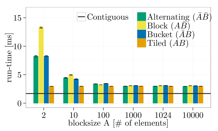
(b) MPI_Bcast, NEC MPI-1.3.1

(c) Ping-pong, NEC MPI-1.3.1

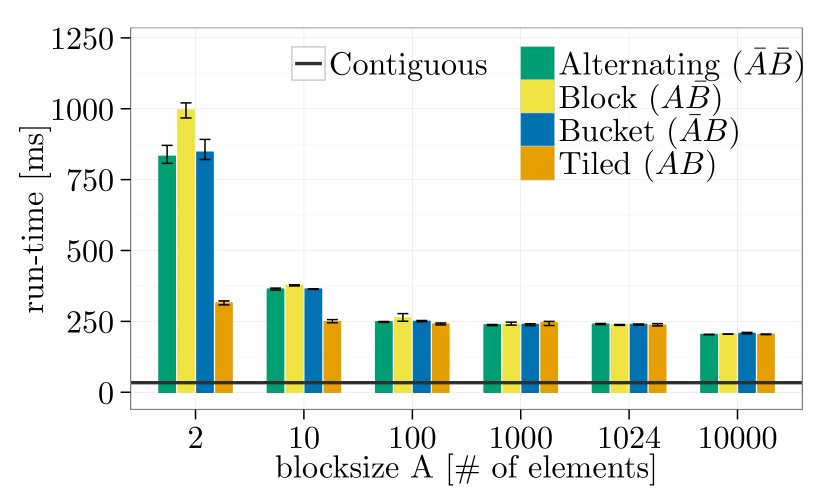
(d) MPI_Allgather, MVAPICH2-2.1

(e) MPI_Bcast, MVAPICH2-2.1

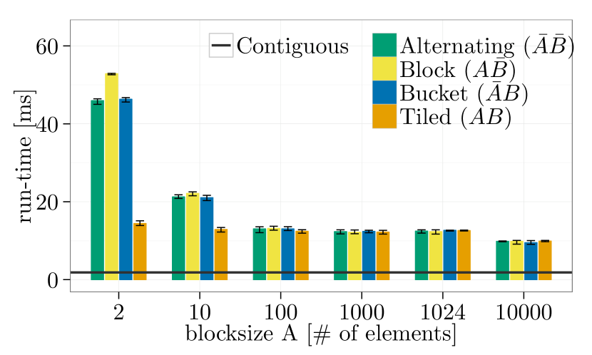
(f) Ping-pong, MVAPICH2-2.1

Figure 2: Contiguous vs. typed, $m=$2.56\text{\,}\mathrm{MB}$$, element datatype: MPI_INT, $32\text{\times}1$ processes ($2\text{\times}1$ for Ping-pong), Variant 1.

We now summarize our findings that characterize the costs of communicating simple, structured data in comparison to communicating the same amount of contiguous data. We have used the basic datatype MPI_INT as the element basetype. We have experimented with two variants for each of the basic layouts, which are summarized in Table 2. All layouts in both variants are defined using the unit size parameter $A$, and the values of the $A$’s and $B$’s are chosen such that all Variant 1 layouts have the same total extent of $n+2n/A$, and all Variant 2 layouts have the same total extent of $3n$.

We describe all experiments by stating the (derived) datatypes used, the reference (baseline) layout against which we evaluate, our expectations (hypotheses) on the performance, and then show and comment on the results.

This gives rise to a very large amount of experimental data, and we cannot show all our results here. A few exemplary results are included in the paper; most other results can be found in the appendix.

2.4.1 Expectation Test 1

This is our basic experiment to measure the “raw” performance of the simple, non-contiguous layouts of Figure 1. We experiment with different message sizes (fixed number of elements in the layouts) and vary the blocksize parameter $A$. We use both variants Variant 1 and Variant 2 for determining the remaining parameters in the layouts.

Experiment

Reference Layout	Contiguous
Compared Layouts	Tiled ($AB$), Block ($A\bar{B}$)
	Bucket ($\bar{A}B$), Alternating ($\bar{A}\bar{B}$)
blocksize $A$	$$2$,$10$,$100$,$1000$,$1024$,$10\,000$$
datasize $m$	$3200\text{\,}\mathrm{B}\mathrm{y}\mathrm{t}\mathrm{e}\mathrm{s}$, $2\,560\,000\text{\,}\mathrm{B}\mathrm{y}\mathrm{t}\mathrm{e}\mathrm{s}$
comm. patterns	Ping-pong, MPI_Bcast, MPI_Allgather
layout variant	1 & 2
# of processes	$32\text{\times}1$, $1\text{\times}16$,
(#nodes $\times$ #cores)	($2\text{\times}1$, $1\text{\times}2$ for Ping-pong)

Type description

We compare the datatype layouts depicted in Figure 1.

Expectations

We expect all communication operations with the non-contiguous layouts to be slower than using the Contiguous layout. We expect this difference to become smaller when increasing the blocksize $A$. It is interesting to find out how large the difference to the contiguous baseline performance is, how the performance is changing between the layouts, how it depends on the type of communication, and whether there are differences between the MPI libraries.

Results

The tiled layout indeed gives the best performance among the four non-contiguous layouts for all three communication patterns. The differences between the layouts are the largest for small values of the blocksize parameter $A$. For all libraries, there is a large difference between process configurations when all MPI processes are on the same node and when they are on different nodes (not shown here, see appendix). For the NEC MPI-1.3.1 library, the performance with non-contiguous data, especially Tiled ($AB$), for processes on the same node is close to the raw performance with contiguous data. The libraries show a large difference in the way they handle non-contiguous data. While the raw performance with contiguous data is comparable among libraries, there is about a factor of two (and more) difference for the non-contiguous layouts, see Figure 2. The NEC MPI-1.3.1 library performs best, as it handles non-contiguous layouts with a tolerable overhead.

2.4.2 Expectation Test 3

MPI provides predefined, basic datatypes corresponding to the basic C and Fortran programing language types. These basic types have different semantic content, and communication performance may differ for data of different basic types. Knowing when this is the case is a valuable information to the application programmer. In particular, we investigate how consecutive buffers consisting of different semantic units perform in comparison to raw, uninterpreted bytes (described by MPI_BYTE).

Experiment

Reference Layout	Contiguous buffer of MPI_BYTE
Compared Layout	Tiled-heterogeneous ($AB\bar{T}$)
blocksize $A$	$$2$,$6$,$8$,$10$,$16$,$100$,$128$,$200$$
stride $B$	$A$
datasize $m$	$48\,000\text{\,}\mathrm{B}\mathrm{y}\mathrm{t}\mathrm{e}\mathrm{s}$, $1\,500\,000\text{\,}\mathrm{B}\mathrm{y}\mathrm{t}\mathrm{e}\mathrm{s}$
comm. patterns	Ping-pong
layout variant	1
# of processes	$2\text{\times}1$, $1\text{\times}2$

Type description

The unit of the Tiled-heterogeneous ($AB\bar{T}$) layout consists of different basetypes $T_{1},T_{2},\ldots$ with blocksize $A$ and stride $B$, where the stride of each block is given in units of the corresponding basetype. The layout is shown in Figure 3. The unit can be described in MPI using MPI_Type_create_struct. It is required that $B\geq A$, where equality is allowed. In our experiments, we use a contiguous layout consisting of MPI_CHAR, MPI_INT, MPI_DOUBLE, MPI_SHORT, with $B=A$ and with $A$ varying between $2$ and $200$.

Figure 3: Contiguous buffer of bytes (MPI_BYTE) (top) vs. Tiled-heterogeneous ($AB\bar{T}$) with $A$=$B$ (bottom).

Expectation

Unless the underlying system indeed requires a different handling of different basic datatypes, we would expect that a contiguous, dense layout of different basic types performs as well as the corresponding amount of unstructured bytes in the MPI communication operations. Since the MPI_Type_create_struct constructor respects alignment constraints for the basic MPI datatypes (in a sense, these are semantic constraints), there might be differences when calling MPI_Type_create_struct to set up the Tiled-heterogeneous layout leads to a non-contiguous layout. This may degrade communication performance.

Results

Our results confirm the hypothesis. The cases with a large difference between the reference and the compared layouts can be explained by alignment constraints that cause the Tiled-heterogeneous layout to become larger than expected, and non-contiguous. This is the same for all three libraries. As the results are not surprising, the corresponding figures are omitted.

2.5 Summary

Our basic layouts can be used to gain insight about the performance when communicating non-contiguous data. We used only two blocksize and stride variants (see Table 2), and observed that the qualitative performance differences are similar. It may thus not be required to check a very large number of other variants. For this reason, we only use the Variant 1 layouts in the next section. It is noteworthy that there are surprisingly large performance differences in handling structured data between the MPI libraries.

3 Performance Expectations

We now investigate relative performance gains (or the opposite) by using MPI derived datatypes, that is, the second and third issue raised in Section 1. We first formulate more precisely what it is reasonable to expect, and benchmark with the aim of verifying or falsifying these expectations. Our expectations take the form of self-consistent performance guidelines [18].

An MPI performance guideline states that a certain MPI operation for some given problem size $n$ should not be slower than some equivalent MPI way of performing the same operation on the same problem size (with all other things being equal). If the MPI operation is slower than the composition of other MPI constructs implementing the same functionality, the operation could be replaced. This is clearly something that an application programmer should not have to do. Verifying such guidelines that interrelate different operations and features of the MPI standard provides a strong means of verifying that a given MPI implementation is “sane”. The verification of a set of guidelines can give valuable hints to the application programmer on how to use features of the MPI standard best.

For MPI datatypes, it seems impossible to say anything absolute about the communication performance for different layouts. But it may well be possible to formulate expectations about how the same layout is handled when it is described with different datatype constructors and different MPI operations.

A first guideline, which is directly derived from the MPI standard [9, Section 4.1.11], states that

$$\mathsf{MPI}\_X(c,t) \simeq \mathsf{MPI}\_X(1,\mathsf{contig}(c,t))$$ (GL1)

excluding the time for setting up and committing the contiguous type on the right-hand side, i.e., an MPI communication operation $X$ should have a similar latency when transferring either $c$ elements of type $t$ or one derived datatype of a contiguous block of $c$ elements. If either side of the equation would be faster than the other, the application programmer could easily switch between them. Thus, it can be expected that an MPI implementation delivers similar performance for both equation sides. As we will see, the argument is not correct, since the MPI_Type_commit operation can perform global optimizations on the contiguous representation of the layout that may lead to a better performance than possible with $c$ repetitions of the block described by $t$. Since this cannot be controlled (or queried) by the application, the two sides of Guideline (GL1) may actually be doing different things.

The next guidelines state that whatever implicit packing and unpacking of non-contiguous data (that may be necessary inside an MPI communication operation) is performed at least as efficiently as explicitly packing and unpacking the whole communication buffer before and after the communication operation using MPI_Pack and MPI_Unpack [9, Section 4.2]. In a good MPI library, we would expect many cases when the left-hand side performs significantly better than the right-hand side. Thus:

$$\mathsf{MPI}\_X(c,t) \preceq \texttt{MPI\_\-Pack}(c,t)+$$ (GL2)

$$\mathsf{MPI}\_X(1,\mathsf{packed}(c,t))$$

for an MPI sending operation $X$, meaning that the performance of the left-hand side is expected to be at least as good as the performance of the right-hand side (all other things being equal). Similarly for an MPI receiving operation $Y$:

$$\mathsf{MPI}\_Y(c,t) \preceq \mathsf{MPI}\_Y(1,\mathsf{packed}(c,t))+$$ (GL3)

$$\texttt{MPI\_\-Unpack}(c,t)$$

The right-hand sides have the disadvantages (1) of requiring an extra buffer for the intermediate, contiguous packing unit, (2) of preventing direct communication of large contiguous parts of the datatype and (3) of preventing pipelining of packing and unpacking in the communication operations (as well as all other dynamic optimizations, and optimizations that exploit communication hardware support). Therefore it should not be recommended. We would expect that MPI libraries trivially fulfill these guidelines with equality, and would hope to find relevant cases where the left-hand sides are much faster than the right-hand sides.

Any data layout can be described in an infinite number of ways with the available MPI datatype constructors. This is easy to see, for instance $\mathsf{contig}(1,t)$ describes the same layout as $t$ itself for any datatype $t$. For any given data layout, each MPI library will have layout descriptions that lead to the best communication performance. The MPI_Type_commit operation provides a handle for the MPI library to transform the datatype given by the user into a better (if possible), internal description. This process is called datatype normalization [3], and we call this best, alternative representation of a layout described by datatype $t$ its normalized form $\mathsf{normal}(t)$. The expectation is that an MPI library will indeed attempt to find a good normalized form at MPI_Type_commit time (if not, the user could do better by deriving the normalized form by himself and setting up the datatype in that way), which is formalized as the following datatype normalization performance guideline:

$$\mathsf{MPI}\_X(c,t) \preceq \mathsf{MPI}\_X(c,\mathsf{normal}(t))$$ (GL4)

That is, we expect the performance of a communication operation $X$ with datatype $t$ to be no worse than what can be achieved with the best, normalized description of the layout. The guideline is tricky, since the user may not readily be able to see what is the best way to describe a layout in a given situation. But in many cases he can give a good guess, and the guideline states that we would expect the MPI_Type_commit operation to do as well.

The normalization heuristics typically applied by MPI libraries replace more general type constructors (struct) with more specific ones (index or index block), collapse nested constructors, and identify large contiguous segments, where such replacements are applicable. Explicit descriptions of common type normalization heuristics can be found in [7, 8, 10, 12, 15]. As we will see in the following, there are natural layout descriptions that are not normalized by these heuristics, leading to severe violations of the guideline.

3.1 Communication Patterns

In our experiments, we will use the same three types of communication operations as in Section 2. In order to verify Guidelines (GL2) and (GL3), we extend the benchmarks with MPI_Pack and MPI_Unpack operations to achieve the same semantics as when datatype arguments were used directly in the communication calls:

1. Ping-pong (cf. Schneider et al. [14]): Ping side: MPI_Pack followed by MPI_Send followed by MPI_Recv followed by MPI_Unpack. Pong side: MPI_Recv followed by MPI_Unpack followed by MPI_Pack followed by MPI_Send.

2. Asymmetric (rooted) collective, e.g., MPI_Bcast on $p$ processes. Root: MPI_Pack followed by MPI_Bcast. Non-roots: MPI_Bcast followed by MPI_Unpack.

3. Symmetric (non-rooted) collective, e.g., MPI_Allgather on $p$ processes. All processes call MPI_Pack, followed by MPI_Allgather, then all processes perform $p$ successive MPI_Unpack operations on the received, packed blocks.

In the MPI_Allgather pattern, the successive unpacking of the received blocks is necessary, since the catenation of packing units is not a packing unit [9, Section 4.2], so even if the received $p$ packed blocks do form a contiguous piece of memory, it is not correct to unpack it with only one MPI_Unpack operation.

3.2 Experimental Results

The structure of experiments is guided by the guidelines, and we state for each experiment what our expectations (hypotheses) are, and comment on whether the results support or falsify them. As baseline we use in most cases the simple layouts of Section 2. We report results only for the MPI_INT basetype and the Variant 1 basic layouts.

3.2.1 Expectation Test 5

For Guidelines (GL2) and (GL3), we first use the layouts of Section 2 with the same values for $A$ and $B$ and compare the benchmark performance with datatype communication against the performance with explicit pack and unpack operations.

Experiment

Reference Layouts	Tiled ($AB$), Block ($A\bar{B}$)
	Bucket ($\bar{A}B$), Alternating ($\bar{A}\bar{B}$)
Compared Layouts	same layouts, but using
	MPI_Pack and MPI_Unpack
blocksize $A$	$$2$,$10$,$10\,000$$
datasize $m$	$64\,000\text{\,}\mathrm{B}\mathrm{y}\mathrm{t}\mathrm{e}\mathrm{s}2\,560\,000\text{\,}\mathrm{B}\mathrm{y}\mathrm{t}\mathrm{e}\mathrm{s}$
comm. patterns	Ping-pong, MPI_Allgather, MPI_Bcast
# of processes	$32\text{\times}1$, $1\text{\times}16$
	($2\text{\times}1$, $1\text{\times}2$ for Ping-pong)

Expectation

We do not expect any MPI library to significantly violate the guidelines Guidelines (GL2) and (GL3) , but with these simple layouts we hope to see cases where an MPI library performs significantly better with datatypes than with explicit packing and unpacking.

Results

(a) Tiled, NEC MPI-1.3.1

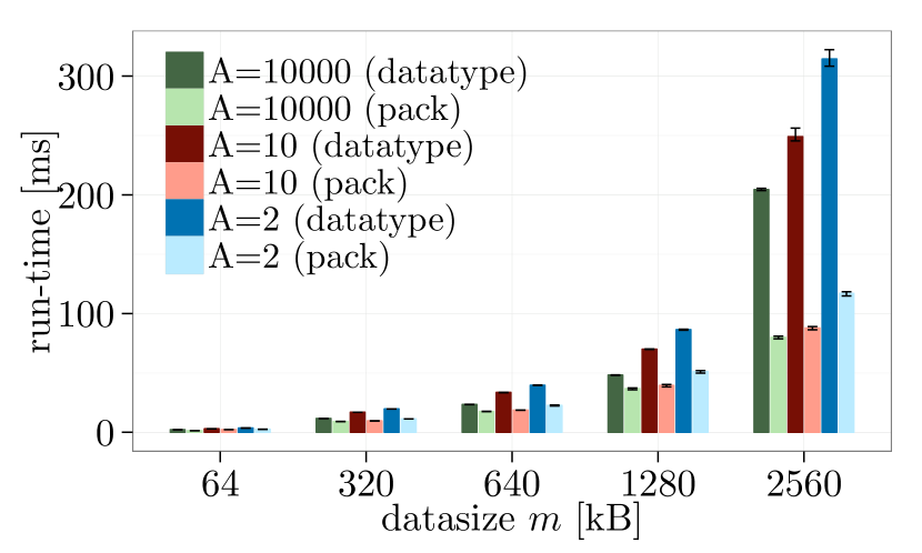
(b) Tiled, MVAPICH2-2.1

(c) Bucket, NEC MPI-1.3.1

(d) Bucket, MVAPICH2-2.1

Figure 4: Basic layouts vs. pack/unpack, element datatype: MPI_INT, $32\text{\times}1$ processes, MPI_Allgather.

(a) NEC MPI-1.3.1

(b) MVAPICH2-2.1

Figure 5: Alternating layout vs. pack/unpack, element datatype: MPI_INT, $1\text{\times}16$ processes, MPI_Bcast.

Much to our surprise, we found many cases where the guidelines are severely violated. For processes on different nodes, both the NEC MPI-1.3.1 and MVAPICH2-2.1 libraries violate the guidelines for all layouts, see Figure 4 for two examples. Especially with MVAPICH2-2.1, the violations are severe and amount to factors of two or more. With MPI processes on the same node, in many cases (with NEC MPI-1.3.1) MPI derived datatypes performed better than explicit packing and unpacking before and after communication. Examples with the MPI_Bcast pattern are shown in Figure 5.

3.2.2 Expectation Test 7

As a sanity check for Guideline (GL1), we create a contiguous $n/k$-element datatype with the MPI_Type_contiguous constructor for each of the $k$-element datatypes of Section 2. We compare the performance of the two datatypes against each other for different communication patterns.

Experiment

Reference Layouts	Tiled ($AB$), Block ($A\bar{B}$)
	Bucket ($\bar{A}B$), Alternating ($\bar{A}\bar{B}$)
Compared Layouts	Contiguous-subtype with subtypes:
	Tiled ($AB$), Block ($A\bar{B}$)
	Bucket ($\bar{A}B$), Alternating ($\bar{A}\bar{B}$)
blocksize $A$	$$2$,$10$,$100$,$1000$,$1024$,$10\,000$$
datasize $m$	$2000\text{\,}\mathrm{B}\mathrm{y}\mathrm{t}\mathrm{e}\mathrm{s}$, $2\,560\,000\text{\,}\mathrm{B}\mathrm{y}\mathrm{t}\mathrm{e}\mathrm{s}$
comm. patterns	Ping-pong
# of processes	$2\text{\times}1$, $1\text{\times}2$

Type description

The concrete Contiguous-subtype is shown in Figure 6 with Tiled ($AB$) as subtype. The Tiled ($AB$) subtype consists of units of $k=A$ elements, and in the communication patterns, $n/k$ such units are communicated. In contrast, the Contiguous-subtype contains all $n/k$ units in a single type, so all $n$ elements are communicated using a count of one with this datatype.

Figure 6: Basic, static layouts (in this figure Tiled ($AB$), top) vs. Contiguous-subtype (bottom).

Expectation

We expect no difference in performance between the reference and compared layouts.

Results

(a) Tiled, NEC MPI-1.3.1

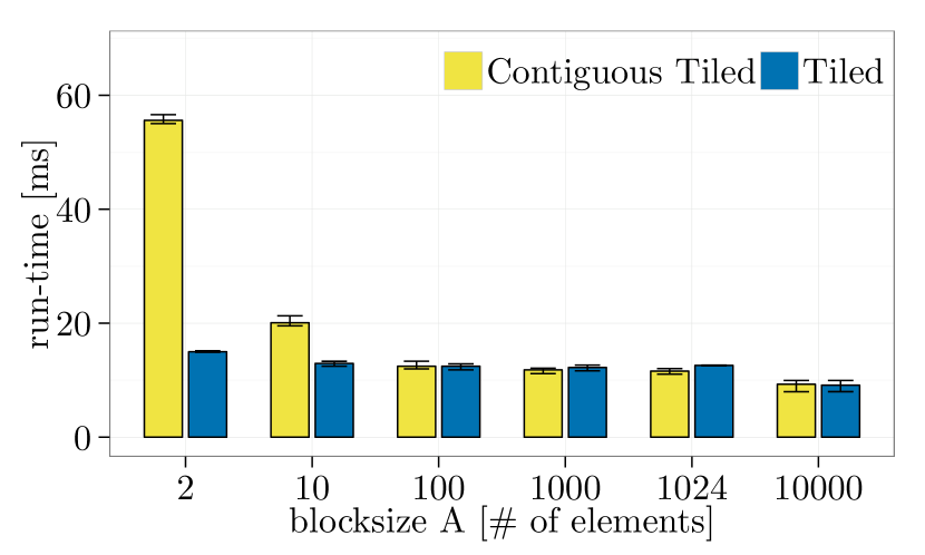
(b) Tiled, MVAPICH2-2.1

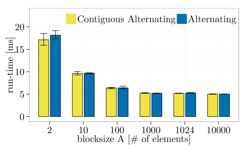
(c) Alternating, NEC MPI-1.3.1

(d) Alternating, MVAPICH2-2.1

Figure 7: Basic layouts vs. Contiguous-subtype, $m=$2.56\text{\,}\mathrm{MB}$$, element datatype: MPI_INT, $2\text{\times}1$ processes, Ping-pong.

Again, surprisingly, the MVAPICH2-2.1 (and also OpenMPI-1.10.1, not shown here) library violates the guideline for the Tiled ($AB$) type, with Contiguous-subtype being a factor of three slower with Tiled ($AB$) as subtype, see Figure 7. For the other basic types Block ($A\bar{B}$), Bucket ($\bar{A}B$), and Alternating ($\bar{A}\bar{B}$), no significant performance difference between the left-hand and the right-hand side of Guideline (GL1) was detected.

3.2.3 Expectation Test 9

The remaining expectation tests are concerned with verifying Guideline (GL4). In all these tests, we give different descriptions of the same layout and study the communication performance. We formulate our expectations (hypotheses) on the assumption that a strong type normalization is not performed by the MPI libraries.

Our first experiment uses the regularly strided Tiled ($AB$) layout, for which we now know the baseline communication performance. We describe this pattern as a larger block comprised of several Tiled ($AB$) subtypes.

Experiment

Reference Layout	Tiled ($AB$)
Compared Layout	Tiled-struct
blocksize $A$	$$2$,$10$,$100$,$1000$,$1024$,$10\,000$$
stride $B$	$A+2$
repetition counts $S_{1},S_{2}$	(a) $S_{1}=1$, $S_{2}=1$
	(b) $S_{1}=2$, $S_{2}=3$
datasize $m$	$2000\text{\,}\mathrm{B}\mathrm{y}\mathrm{t}\mathrm{e}\mathrm{s}$, $2\,560\,000\text{\,}\mathrm{B}\mathrm{y}\mathrm{t}\mathrm{e}\mathrm{s}$
comm. patterns	Ping-pong
# of processes	$2\text{\times}1$, $1\text{\times}2$

Type description

The Tiled-struct layout is a concatenation described with MPI_Type_create_struct of two smaller, contiguously strided layouts of $S_{1}$ and $S_{2}$ tiled blocks. The description is illustrated in Figure 8. Each Tiled sub-layout has the same blocksize $A$ and stride $B$. The number of elements in the structure is $(S_{1}+S_{2})A$. We also allow the degenerated (fully contiguous) case of $A=B$. However, we only test the performance of the structured layout using $A<B$, with $A$ and $B$ chosen as in Variant 1 (cf. Table 2).

Figure 8: Tiled (top) vs. Tiled-struct (bottom).

Expectation

As explained, since the user can easily describe the Tiled layout with the MPI_Type_contiguous and MPI_Type_create_resized constructor, we would like to expect that the MPI library can detect from the Tiled-struct description that the underlying pattern is a simple, tiled pattern. That would require detecting that both sub-layouts of the MPI_Type_create_struct are indeed tiled (although with different repetition counts) and have the same basetype. However, the heuristics used by MPI libraries at MPI_Type_commit time usually work differently [7, 8]. Therefore, we actually expect to see cases where the Tiled-struct description performs worse than the reference layout.

Results

(a) NEC MPI-1.3.1

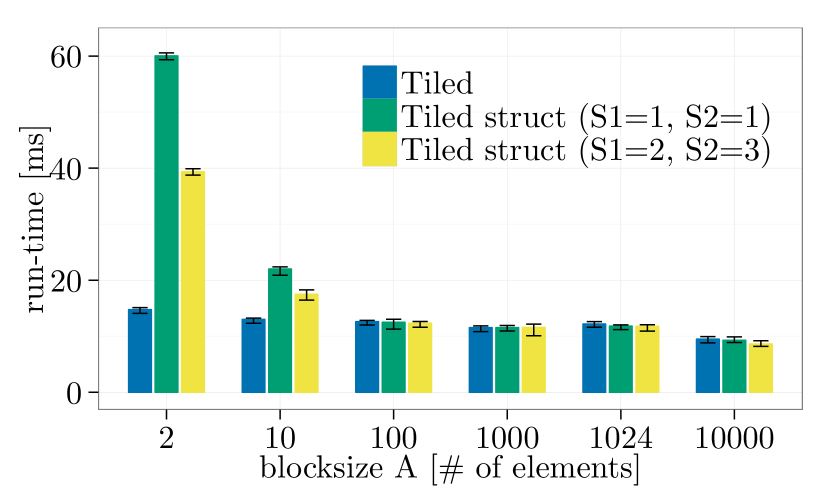
(b) MVAPICH2-2.1

Figure 9: Tiled ($AB$) vs. Tiled-struct, element datatype: MPI_INT, $m=$2.56\text{\,}\mathrm{MB}$$, $2$ nodes, Ping-pong.

The results in Figure 9, especially for MVAPICH2-2.1, show a large performance difference for $A=2$. Even in the case of $S_{1}=S_{2}$, where the two subtypes are identically set up, the Tiled-struct performs several factors worse. This shows that the normalization heuristics in the MPI libraries are insufficient to identify the complex description of the simple, tiled layout and to normalize accordingly.

3.2.4 Expectation Test 11

The next experiment for Guideline (GL4) is also a sanity check, where we would expect no differences between two equally simple, natural descriptions of a tiled layout. We now describe the Tiled ($AB$) layout as a vector of $n/A$ contiguous blocks of $A$ elements with stride $B$. This is the “most natural” way in MPI to describe a long, regularly strided layout, and is accomplished with MPI_Type_vector. To have the same extent of the vector type, we resize the extent of the vector to $n/A$ times the extent of Tiled ($AB$). The Tiled-vector datatype is our first example of a dynamically derived datatype that can only be set up when the number of elements $n$ to be communicated is known. As in all our experiments, we do not include the datatype setup time in the measured run-time.

Experiment

Reference Layout	Tiled ($AB$)
Compared Layout	Tiled-vector
blocksize $A$	$$2$,$10$,$100$,$1000$,$1024$,$10\,000$$
stride $B$	$A+2$
datasize $m$	$2000\text{\,}\mathrm{B}\mathrm{y}\mathrm{t}\mathrm{e}\mathrm{s}$, $2\,560\,000\text{\,}\mathrm{B}\mathrm{y}\mathrm{t}\mathrm{e}\mathrm{s}$
comm. patterns	Ping-pong
# of processes	$2\text{\times}1$, $1\text{\times}2$

Type description

The two contrasted datatype layout descriptions Tiled ($AB$) and Tiled-vector are illustrated in Figure 10.

Figure 10: Tiled-vector defines the layout with MPI_Type_vector using the Tiled pattern.

Expectation

We expect the performance of the two descriptions to match. The MPI internal representations of the two descriptions can be expected to be similar, and concrete offsets for accessing the elements in the layout can be computed easily by the datatype engine given these representations. Since the MPI_Type_vector is a commonly used datatype constructor, it may even have been specially optimized, such that the description as Tiled-vector might be slightly advantageous.

Results

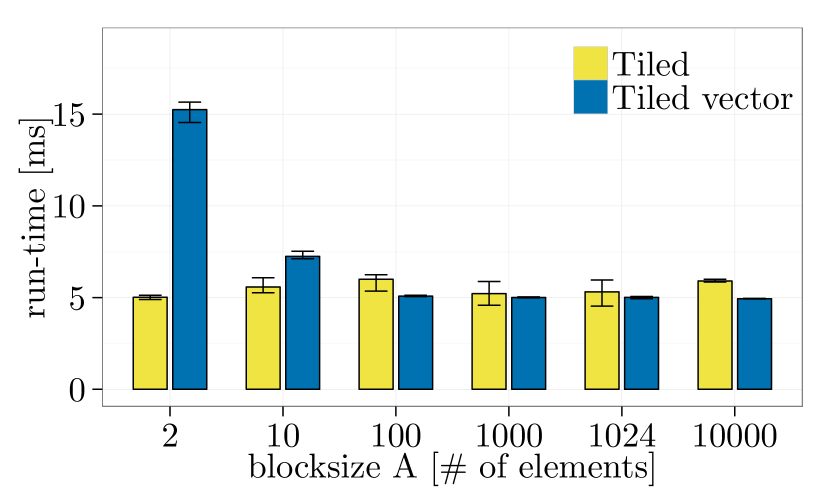
(a) NEC MPI-1.3.1

(b) MVAPICH2-2.1

Figure 11: Tiled ($AB$) vs. Tiled-vector, element datatype: MPI_INT, $m=$2.56\text{\,}\mathrm{MB}$$, $2$ nodes, Ping-pong.

As shown in Figure 11, for the NEC MPI-1.3.1 (and also for OpenMPI-1.10.1) library and small values of $A$, the Tiled-vector performs much worse than repeating the Tiled ($AB$) block. This is again surprising. However, the comparison of the absolute performance between NEC MPI-1.3.1 and MVAPICH2-2.1 shows that the bad performance of Tiled-vector is relative, in absolute terms it is on par with the performance in MVAPICH2-2.1 for both descriptions of the layout. These findings also illustrate that performance guidelines can only ensure consistency in an MPI library. Guideline verification needs to be complemented with benchmarking against hard baselines.

3.2.5 Expectation Test 13

Our next description of the Tiled ($AB$) layout is done using a nested vector. We describe a larger block of a constant $S$ number of units of $A$ elements and stride $B$ with the MPI_Type_vector constructor. On this datatype, we build a dynamic vector of $n/(SA)$ blocks with a stride of $SB$ elements. In order to express the stride correctly, this vector has to be constructed with the MPI_Type_hvector constructor.

Experiment

Reference Layout	Tiled ($AB$)
Compared Layout	Vector-tiled
blocksize $A$	$$2$,$10$,$100$,$1000$,$1024$,$10\,000$$
stride $B$	$A+2$
datasize $m$	$2000\text{\,}\mathrm{B}\mathrm{y}\mathrm{t}\mathrm{e}\mathrm{s}$, $2\,560\,000\text{\,}\mathrm{B}\mathrm{y}\mathrm{t}\mathrm{e}\mathrm{s}$
comm. patterns	Ping-pong
# of processes	$2\text{\times}1$, $1\text{\times}2$

Type description

The setup of the nested vector Vector-tiled versus the basic layout Tiled ($AB$) is illustrated in Figure 12.

Figure 12: Vector-tiled

Expectation

We expect that an MPI library will detect that the stride for the outer vector is equal to $c$ times the stride of the inner vector, such that the layout can also be described by a non-nested vector constructor. MPI_Type_commit should perform the transformation. The performance of the two descriptions should therefore be similar, regardless of the communication pattern.

Results

(a) NEC MPI-1.3.1

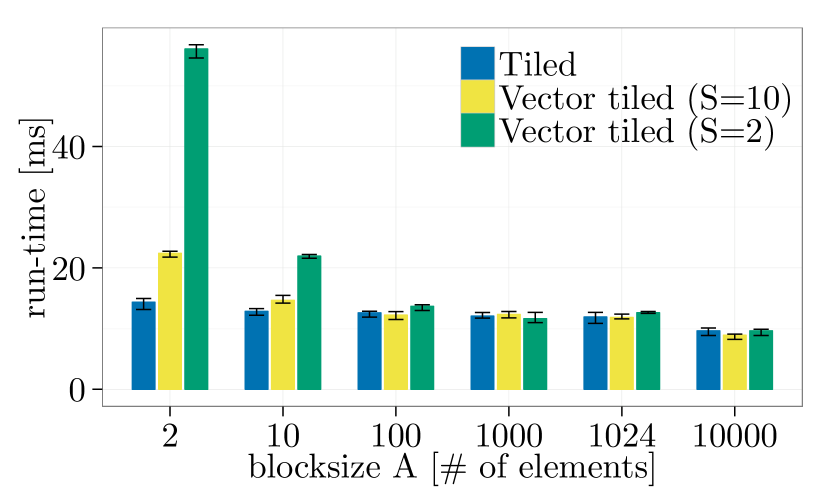
(b) MVAPICH2-2.1

Figure 13: Tiled ($AB$) vs. Vector-tiled, element datatype: MPI_INT, $m=$2.56\text{\,}\mathrm{MB}$$, $2$ nodes, Ping-pong.

To our surprise, apparently none of the MPI libraries normalizes the two-level nested vector description into a better layout. For a small unit of size $A=2$, the communication time with Vector-tiled compared to the communication time with the simple Tiled ($AB$) description differ by factors from 2 to 4, as shown in Figure 13.

3.2.6 Expectation Test 15

In this experiment, we look at different, explicit descriptions of the more irregular layout Block ($A\bar{B}$), by explicitly listing the displacements and number of elements in all $n/k$ blocks in the $n$ element layouts. The purpose of this experiment is to investigate the relative penalty of having to traverse long, explicit lists of displacements, versus implicit, computed displacements.

Experiment

Reference Layout	Block ($A\bar{B}$)
Compared Layout	Block-indexed
blocksize $A$	$$2$,$10$,$100$,$1000$,$1024$,$10\,000$$
stride $B$	$B_{1}=A+1$, $B_{2}=A+3$
datasize $m$	$3200\text{\,}\mathrm{B}\mathrm{y}\mathrm{t}\mathrm{e}\mathrm{s}$, $2\,560\,000\text{\,}\mathrm{B}\mathrm{y}\mathrm{t}\mathrm{e}\mathrm{s}$
comm. patterns	Ping-pong
# of processes	$2\text{\times}1$, $1\text{\times}2$

Type description

The Block-indexed layout uses the Block layout with given $A,B_{1}$, and $B_{2}$, described with the MPI_Type_create_indexed_block constructor with $n/A$ indices and blocksize $A$. The block displacements can easily be computed. This is illustrated in Figure 14.

Figure 14: Static Block ($A\bar{B}$) (top) vs. dynamic Block-indexed (bottom) description of the Block ($A\bar{B}$) layout.

Expectation

An MPI library should normalize both cases to the same internal datatype representation with good performance. It is doubtful that anything like that will happen. More importantly, it is not obvious which of the two descriptions is better. A reasonable expectation is that beyond some number of elements, the large array of displacements (indices) in the Block-indexed datatype will become expensive to traverse, and that simple repetitions of the small, irregular non-contiguous Block pattern will perform better.

Results

For small blocksizes of $A$, the Block description is worse, especially for the NEC MPI-1.3.1 library. Otherwise the performance of the two descriptions looks similar. Nevertheless, the absolute performance of the NEC MPI-1.3.1 library is still better. We do not show the results here (see appendix).

3.2.7 Expectation Test 17

This experiment is similar to the previous one. Here, two descriptions of the “most irregular” of the four basic layouts, namely Alternating ($\bar{A}\bar{B}$) are contrasted.

Experiment

Reference Layout	Alternating ($\bar{A}\bar{B}$)
Compared Layout	Alternating-indexed
blocksize $A$	$$2$,$10$,$100$,$1000$,$1024$,$10\,000$$
blocksizes $A_{1}$, $A_{2}$	$A_{1}=A-1$, $A_{2}=A+1$
stride $B$	$B_{1}=A+1$, $B_{2}=A+3$
datasize $m$	$3200\text{\,}\mathrm{B}\mathrm{y}\mathrm{t}\mathrm{e}\mathrm{s}$, $2\,560\,000\text{\,}\mathrm{B}\mathrm{y}\mathrm{t}\mathrm{e}\mathrm{s}$
comm. patterns	Ping-pong
# of processes	$2\text{\times}1$, $1\text{\times}2$

Type description

The Alternating-indexed datatype is based on the Alternating layout with given $A_{1},A_{2},B_{1}$, and $B_{2}$, described with the MPI_Type_indexed constructor with $n/(A_{1}+A_{2})$ indices and blocksizes of $A_{1}$ and $A_{2}$. The data layout is illustrated in Figure 15.

Figure 15: Static Alternating ($\bar{A}\bar{B}$) (top) vs. dynamic Alternating-indexed (bottom) description of the Alternating ($\bar{A}\bar{B}$) layout.

Expectation

As for the previous experiment, it is not obvious which of the two descriptions will perform better (under the pessimistic assumption that no normalization takes place). Experimental results will give insight on whether there is a penalty for large lists of displacements in the MPI_Type_indexed constructor.

Results

For larger values of $A$, the performance of the two descriptions looks similar. For small values of $A$, the results are the opposite of the previous experiment. Especially for the NEC MPI-1.3.1, the Alternating-indexed description performs worse than the Alternating ($\bar{A}\bar{B}$) description. Results are not shown here (see appendix).

3.2.8 Expectation Test 19

In our final test with the basic layouts, we look at an Alternating ($\bar{A}\bar{B}$) pattern where the stride $B_{2}$ of the second unit is equal to the number of elements $A_{2}$ in the unit. This pattern can be described as a repetition of small datatypes describing fixed blocks. It can alternatively be formulated as a layout comprised of (1) a first, small unit of $A_{1}$ elements, (2) a large, regularly strided middle part, and (3) a last, small unit of $A_{2}$ elements. We expect the second description to perform better, and we want to check this hypothesis.

Experiment

Compared Layouts	Alternating-repeated
	Alternating-struct
blocksize $A$	$$2$,$10$,$100$,$1000$,$1024$,$10\,000$$
unit blocksizes $A_{1}$, $A_{2}$	$A_{1}=A-1$, $A_{2}=A+1$
stride $B$	$A+1$
datasize $m$	$3200\text{\,}\mathrm{B}\mathrm{y}\mathrm{t}\mathrm{e}\mathrm{s}$, $2\,560\,000\text{\,}\mathrm{B}\mathrm{y}\mathrm{t}\mathrm{e}\mathrm{s}$
comm. patterns	Ping-pong
# of processes	$2\text{\times}1$, $1\text{\times}2$

Type description

Here, two types describe an alternating layout with units of $A_{1}$ and $A_{2}$ elements and strides $B_{1}=B$ and $B_{2}=A_{2}$, respectively. The first datatype is called Alternating-repeated and is defined as a fixed, alternating block (Figure 16a). The second is called Alternating-struct and is created with MPI_Type_create_struct using three subtypes: the first is a block of $A_{1}$ contiguous elements, the second subtype is a tiled vector, and the third subtype is a contiguous block of $A_{2}$ elements (Figure 16b).

Figure 16: Alternating-repeated (top) vs. Alternating-struct (bottom).

Expectation

With the description as an Alternating-struct, communication performance should approach the performance of communicating a tiled vector with blocksizes of $A_{1}+A_{2}$ elements, when the total number of elements $n$ goes up. Our previous measurements have given the baseline performance for such Tiled ($AB$) patterns, against which we can compare. Since commonly used MPI normalization heuristics do probably not change the description from Alternating-repeated to the possibly better Alternating-struct, our expectation is that the latter will perform better.

Results

(a) NEC MPI-1.3.1

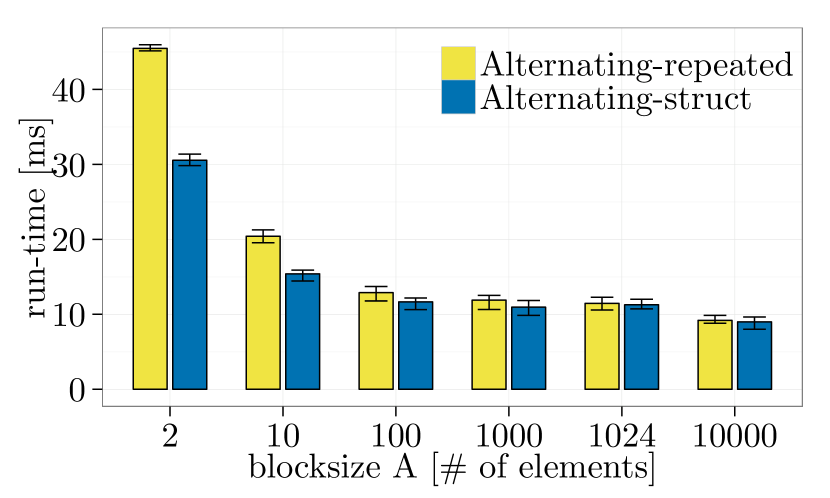
(b) MVAPICH2-2.1

Figure 17: Alternating-repeated vs. Alternating-struct, element datatype: MPI_INT, $m=$2.56\text{\,}\mathrm{MB}$$, $2$ nodes, Ping-pong.

For small values of $A$, the Alternating-repeated way of communicating the pattern is indeed slower for all tested MPI libraries; see Figure 17. This shows that a stronger type normalization (on the fly) than currently performed by MPI libraries is needed to approach the baseline performance. It also shows, and this is important, that the MPI_Type_create_struct constructor is needed for the best description even of homogeneous layouts where all elements have the same basic type.

3.2.9 Expectation Test 21

For our final set of experiments, we use another layout. Given an $(n+1-A)\times A$ matrix, we want to communicate together the first row of $A$ elements and the (remainder of the) first column of $n-A$ elements, for a total of $n$ elements. For examining Guideline (GL4), we again compare natural ways of describing this layout, and compare the measured communication times. A similar example was used by Ganian et al. [2].

Experiment

Compared Layouts	RowCol-fully-indexed
	RowCol-contiguous-and-indexed
	RowCol-struct
blocksize $A$	$$2$,$10$,$100$,$128$,$512$,$1000$,$1024$,$5000$,$10\,000$$
# of elements $n$	$$100$,$10\,240$$
comm. patterns	Ping-pong
# of processes	$2\text{\times}1$, $1\text{\times}2$

Type description

A row-column layout (submatrix of $(n+1-A)\times A$ matrix), consisting of $A$ consecutive elements followed by $n-A$ elements in a strided layout with stride $A$, can be described either by

1. using MPI_Type_create_indexed_block with $n$ indices (RowCol-fully-indexed),

2. using MPI_Type_indexed with $1+n-A$ indices (RowCol-contiguous-and-indexed), or

3. using MPI_Type_create_struct consisting of a contiguous subtype of $A$ elements, followed by a vector of $n-A$ blocks of one element with stride $A$ (RowCol-struct).

The layout and the three possible descriptions as derived datatypes are shown in Figure 18.

Figure 18: From left to right: RowCol-fully-indexed, RowCol-contiguous-and-indexed, RowCol-struct.

Expectation

The latter representation is the most compact, and expectedly best performing. This layout description also illustrates that the full power of the MPI_Type_create_struct constructor is needed, even for homogeneous layouts of elements of the same basic type. As we do not expect the MPI libraries to perform a normalization into an efficient data representation, our hypothesis is that the RowCol-struct datatype will perform better than the two other types, and that RowCol-contiguous-and-indexed may perform better than RowCol-fully-indexed as the blocksize $A$ goes up.

Results

(a) NEC MPI-1.3.1

(b) MVAPICH2-2.1

Figure 19: RowCol-fully-indexed, RowCol-contiguous-and-indexed, RowCol-struct, element datatype: MPI_INT, $n=$10\,240$$, extent increases with $A$, $2$ nodes, Ping-pong.

The results in Figure 19 confirm that for NEC MPI-1.3.1 the compact description RowCol-struct gives the best performance, closely followed by RowCol-fully-indexed. For the MVAPICH2-2.1, the performance is worse (compared to NEC MPI-1.3.1 as baseline) for all three descriptions, except for large values of $A$. The results for OpenMPI-1.10.1 (see appendix) are as expected, with the compact RowCol-struct description being close to a factor of two faster than the other two (except for the large $A$ values).

4 Summmary and Outlook

We performed a large number of experiments to explore the performance of communication with differently structured, non-contiguous data layouts described by MPI derived datatypes. We focused on simple tiled layouts parameterized by element counts and strides, and structured the experiments as a set of expectation tests using MPI performance guidelines.

The results were revealing and in many cases surprising and disappointing. For instance, it was unexpected that Guidelines (GL2) and (GL3) would be violated, but we found many cases (for all libraries) where these guidelines were severely compromised. In such cases, the recommendation to use datatypes is hard to justify. It is definitely important to look into the reasons and improve the situation. We also observe that the communication performance with (non-trivial) derived datatypes is quite different between the libraries. For example, the current version of MVAPICH does not handle derived datatypes as efficiently as the other libraries.

In addition, the simplest expectations concerning the use of the MPI_Type_contiguous constructor, captured in Guideline (GL1), were sometimes violated. We believe that these violations can and should be repaired.

Our experiments around Guideline (GL4) first and foremost show that the way a given layout is described as a derived datatype matters a lot. Or put differently, the heuristics employed by common MPI libraries in MPI_Type_commit are insufficient to find good internal datatype representations. It is worthwhile to improve the situation, since an application programmer currently needs a good intuition to select an efficient derived datatype description. Simple rules of thumb are not enough: our findings sometimes contradicted our own intuitions and expectations. Furthermore, some experiments show that datatype descriptions may be too localized to make a sufficiently good normalization possible, namely, that both the repetition count and the datatype are needed for computing the normalized type description. However, normalization on the fly in each communication call is not an option for a high-performance MPI library, especially since (optimal) normalization may be very expensive [2]. Therefore, the performance equivalence of the seemingly innocent Guideline (GL1) cannot hold when MPI_Type_commit may normalize the contiguous type (right-hand side of the guideline). MPI might need more query functionality for the application programmer to explore and guide the normalization.

5 Acknowledgments

We thank Antoine Rougier and Felix Donatus Lübbe (TU Wien) for helping us with some of the experiments.

This appendix contains our currently full set of experiments, only some of which are shown in the main text. The results are listed in the order of the expectation tests.

Appendix A Experimental Results

A.1 Expectation Test 2.4.1 (Sect. 2.4.1)

 

• Contiguous, Tiled ($AB$), Block ($A\bar{B}$), Bucket ($\bar{A}B$), Alternating ($\bar{A}\bar{B}$)

• Ping-pong, MPI_Bcast, MPI_Allgather

 

• Figure 20:   NEC MPI-1.3.1, small datasize, Variant 1

• Figure 21:   MVAPICH2-2.1, small datasize, Variant 1

• Figure 22:   OpenMPI-1.10.1, small datasize, Variant 1

• Figure 23:   NEC MPI-1.3.1, large datasize, Variant 1

• Figure 24:   MVAPICH2-2.1, large datasize, Variant 1

• Figure 25:   OpenMPI-1.10.1, large datasize, Variant 1, one node

• Figure 26:   NEC MPI-1.3.1, small datasize, Variant 1, one node

• Figure 27:   MVAPICH2-2.1, small datasize, Variant 1, one node

• Figure 28:   OpenMPI-1.10.1, small datasize, Variant 1, one node

• Figure 29:   NEC MPI-1.3.1, large datasize, Variant 1, one node

• Figure 30:   MVAPICH2-2.1, large datasize, Variant 1, one node

• Figure 31:   OpenMPI-1.10.1, large datasize, Variant 1, one node

• Figure 32:   MVAPICH2-2.1, small datasize, Variant 2

• Figure 33:   MVAPICH2-2.1, large datasize, Variant 2

• Figure 34:   MVAPICH2-2.1, small datasize, Variant 2, one node

• Figure 35:   MVAPICH2-2.1, large datasize, Variant 2, one node

 

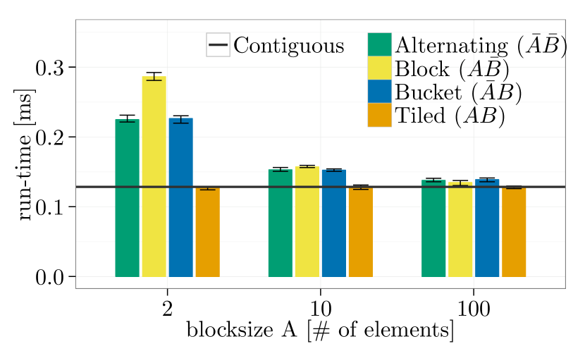
(a) MPI_Allgather

(b) MPI_Bcast

(c) Ping-pong

Figure 20: Contiguous vs. typed, $m=$3.2\text{\,}\mathrm{kB}$$, element datatype: MPI_INT, $32\text{\times}1$ processes ($2\text{\times}1$ for Ping-pong), NEC MPI-1.3.1, Variant 1.

(a) MPI_Allgather

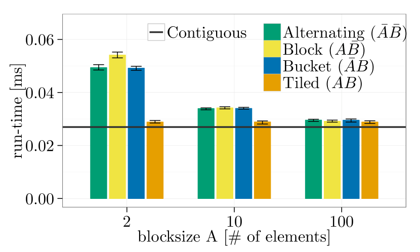
(b) MPI_Bcast

(c) Ping-pong

Figure 21: Contiguous vs. typed, $m=$3.2\text{\,}\mathrm{kB}$$, element datatype: MPI_INT, $32\text{\times}1$ processes ($2\text{\times}1$ for Ping-pong), MVAPICH2-2.1, Variant 1.

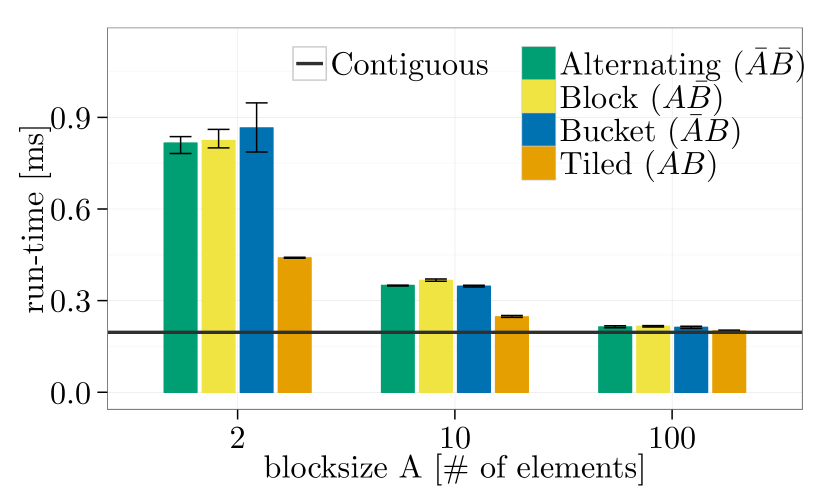
(a) MPI_Allgather

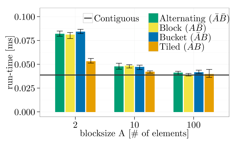
(b) MPI_Bcast

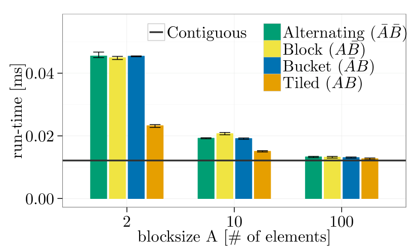
(c) Ping-pong

Figure 22: Contiguous vs. typed, $m=$3.2\text{\,}\mathrm{kB}$$, element datatype: MPI_INT, $32\text{\times}1$ processes ($2\text{\times}1$ for Ping-pong), OpenMPI-1.10.1, Variant 1.

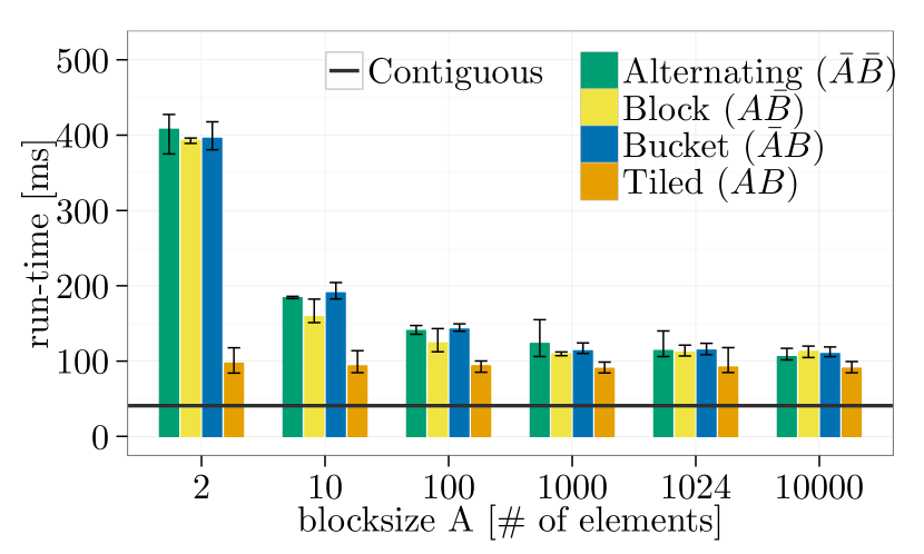
(a) MPI_Allgather

(b) MPI_Bcast

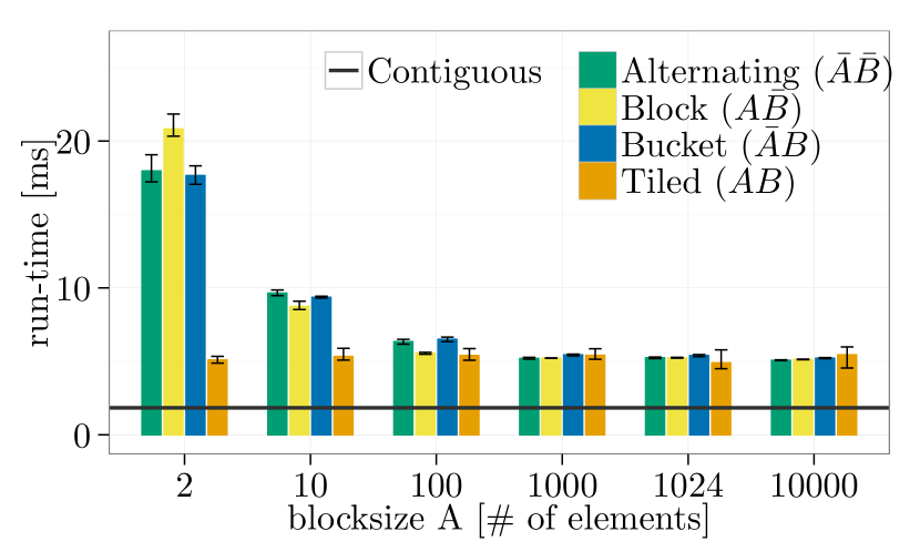
(c) Ping-pong

Figure 23: Contiguous vs. typed, $m=$2.56\text{\,}\mathrm{MB}$$, element datatype: MPI_INT, $32\text{\times}1$ processes ($2\text{\times}1$ for Ping-pong), NEC MPI-1.3.1, Variant 1.

(a) MPI_Allgather

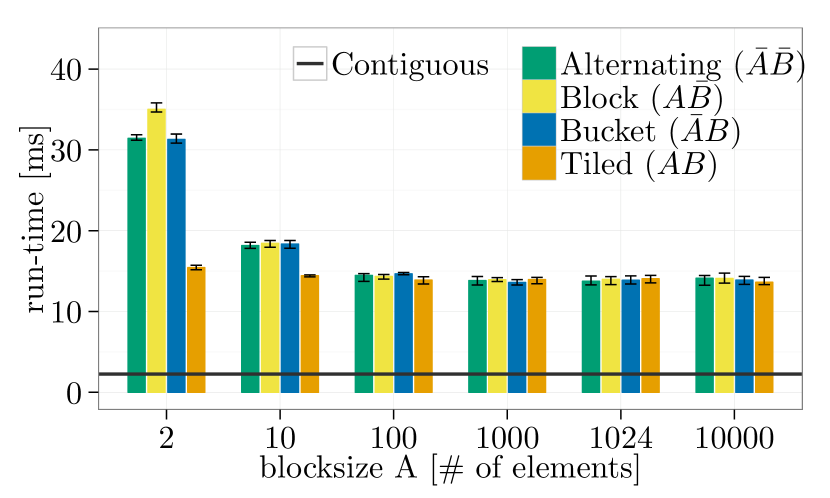
(b) MPI_Bcast

(c) Ping-pong

Figure 24: Contiguous vs. typed, $m=$2.56\text{\,}\mathrm{MB}$$, element datatype: MPI_INT, $32\text{\times}1$ processes ($2\text{\times}1$ for Ping-pong), MVAPICH2-2.1, Variant 1.

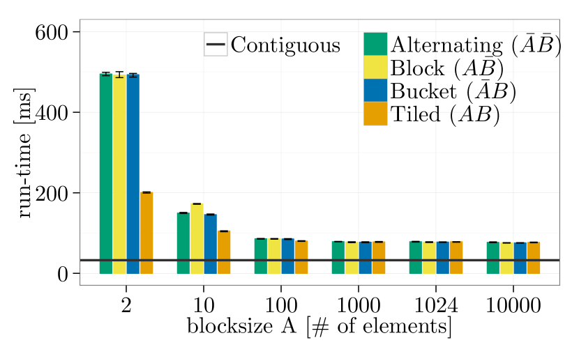
(a) MPI_Allgather

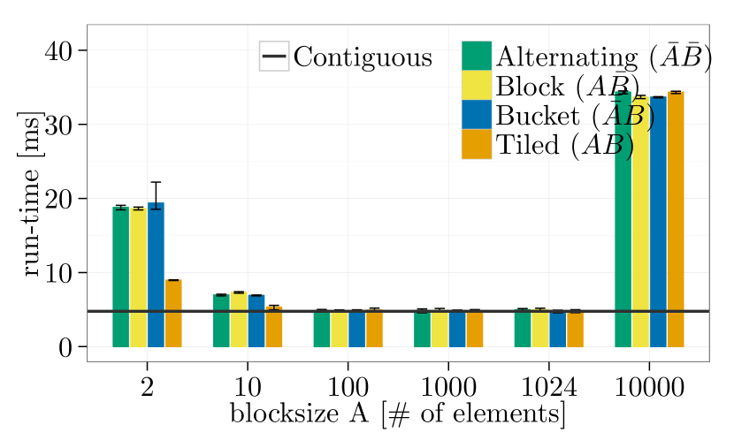
(b) MPI_Bcast

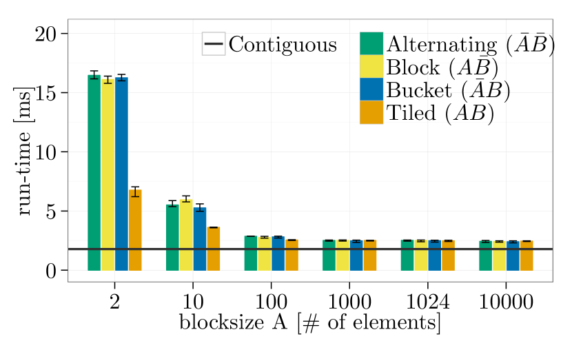
(c) Ping-pong

Figure 25: Contiguous vs. typed, $m=$2.56\text{\,}\mathrm{MB}$$, element datatype: MPI_INT, $32\text{\times}1$ processes ($2\text{\times}1$ for Ping-pong), OpenMPI-1.10.1, Variant 1.

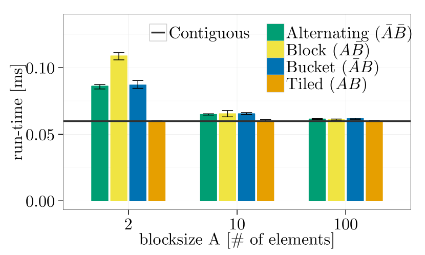
(a) MPI_Allgather

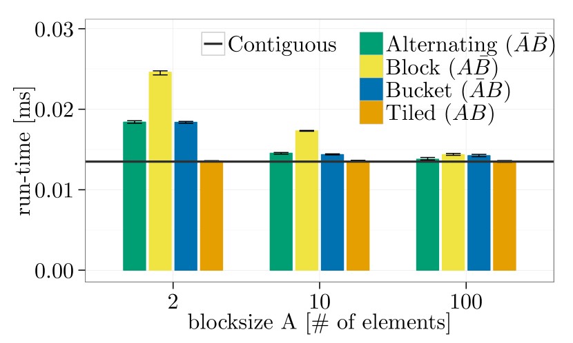
(b) MPI_Bcast

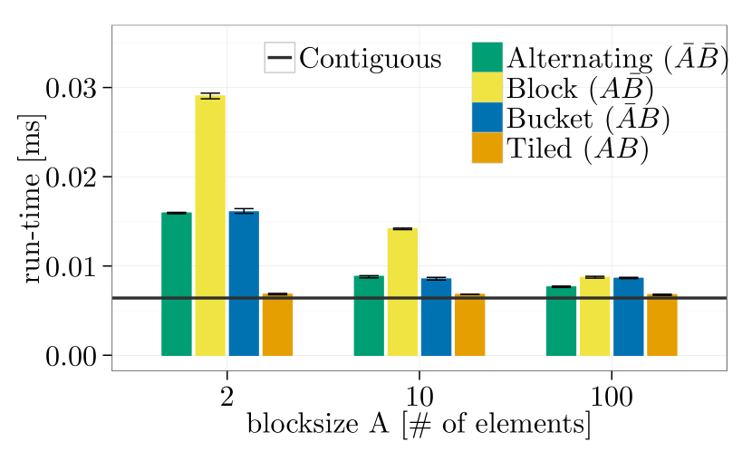
(c) Ping-pong

Figure 26: Contiguous vs. typed, $m=$3.2\text{\,}\mathrm{kB}$$, element datatype: MPI_INT, one node, $16$ processes ($2$ for Ping-pong), NEC MPI-1.3.1, Variant 1.

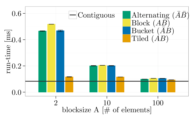
(a) MPI_Allgather

(b) MPI_Bcast

(c) Ping-pong

Figure 27: Contiguous vs. typed, $m=$3.2\text{\,}\mathrm{kB}$$, element datatype: MPI_INT, one node, $16$ processes ($2$ processes for Ping-pong), MVAPICH2-2.1, Variant 1.

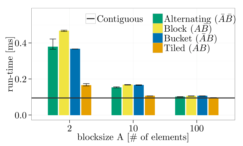
(a) MPI_Allgather

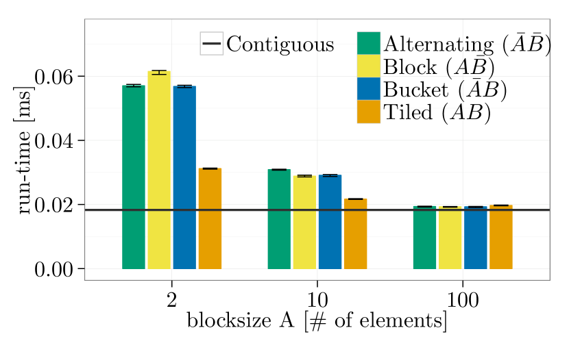
(b) MPI_Bcast

(c) Ping-pong

Figure 28: Contiguous vs. typed, $m=$3.2\text{\,}\mathrm{kB}$$, element datatype: MPI_INT, $1$ node, $16$ processes ($2$ processes for Ping-pong), OpenMPI-1.10.1, Variant 1.

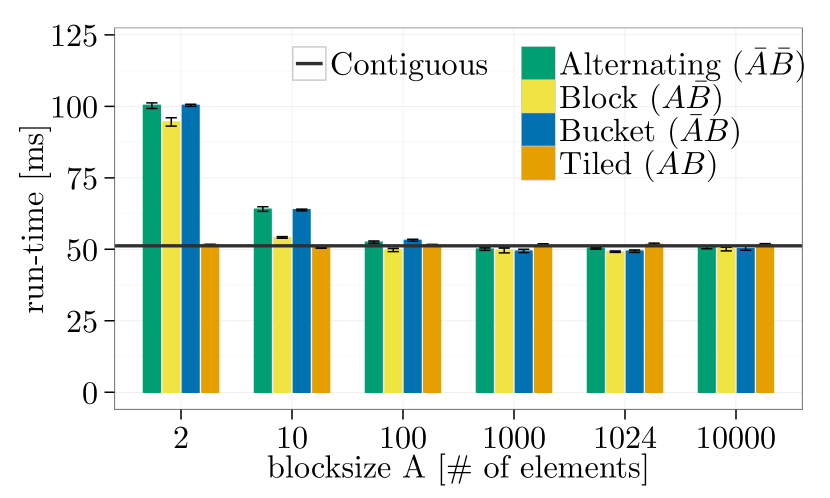
(a) MPI_Allgather

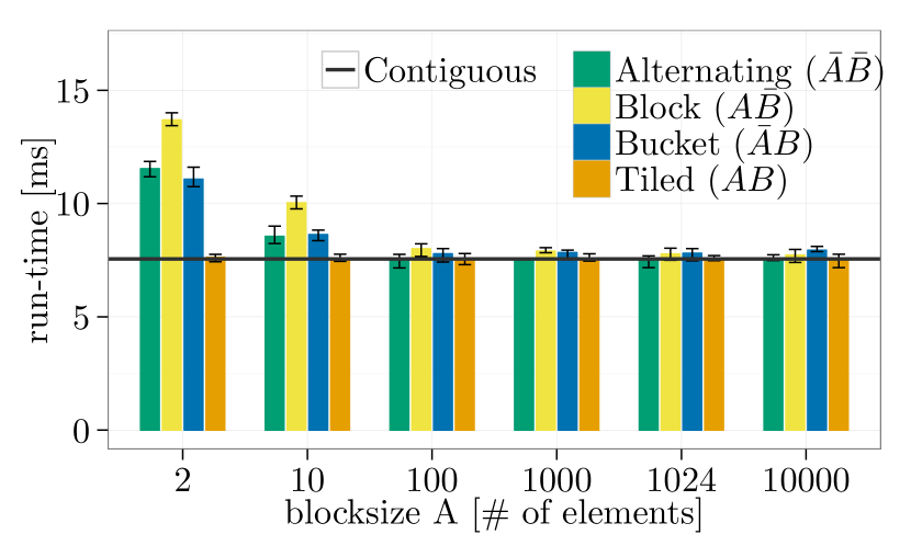
(b) MPI_Bcast

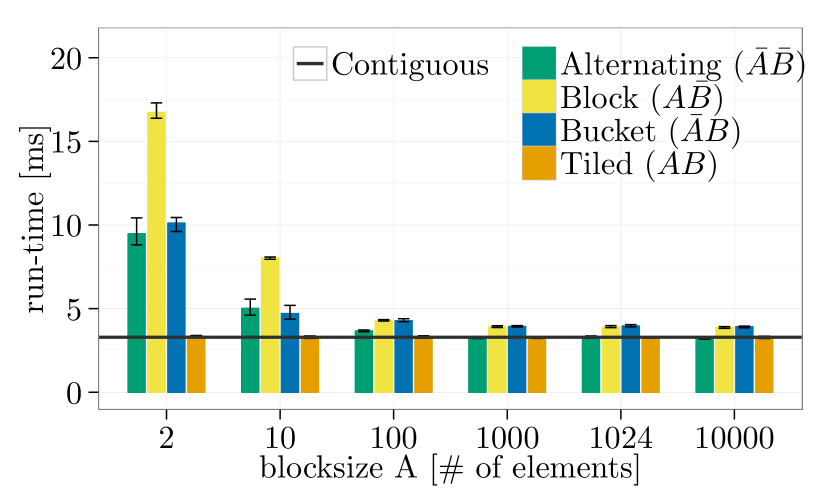
(c) Ping-pong

Figure 29: Contiguous vs. typed, $m=$2.56\text{\,}\mathrm{MB}$$, element datatype: MPI_INT, one node, $16$ processes ($2$ processes for Ping-pong), NEC MPI-1.3.1, Variant 1.

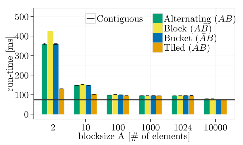
(a) MPI_Allgather

(b) MPI_Bcast

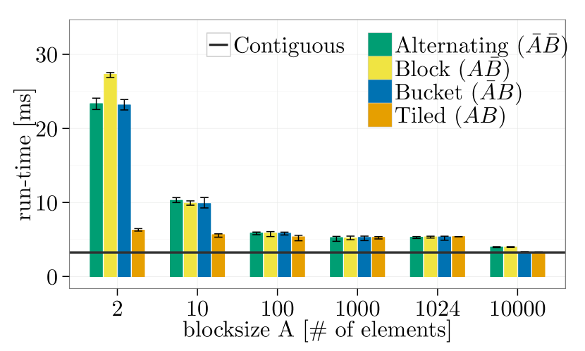
(c) Ping-pong

Figure 30: Contiguous vs. typed, $m=$2.56\text{\,}\mathrm{MB}$$, element datatype: MPI_INT, one node, $16$ processes ($2$ processes for Ping-pong), MVAPICH2-2.1, Variant 1.

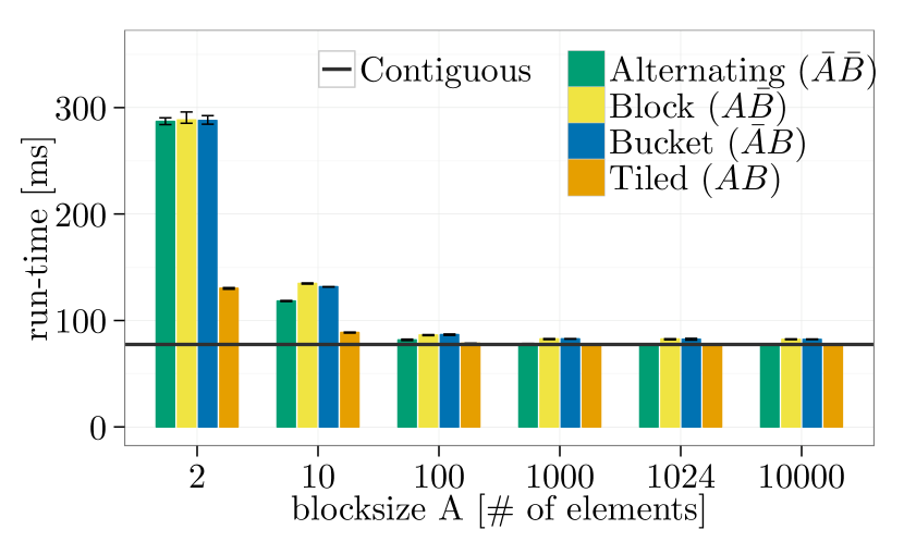
(a) MPI_Allgather

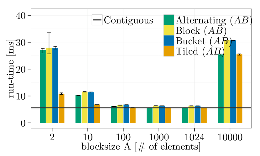
(b) MPI_Bcast

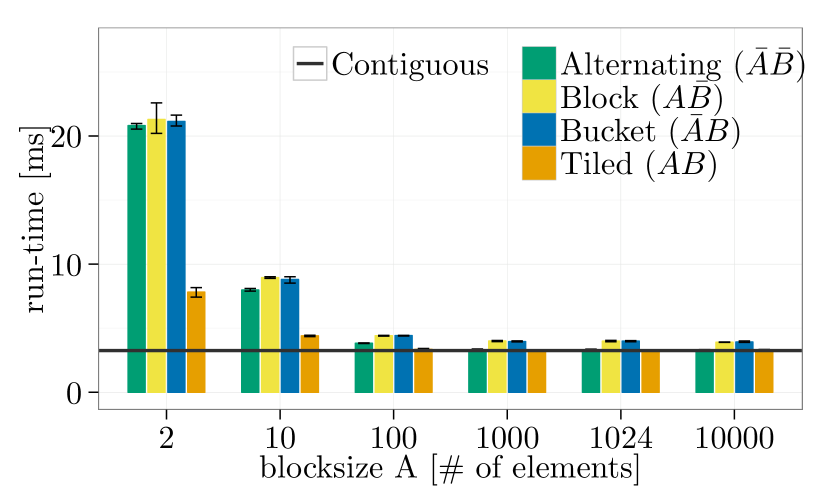
(c) Ping-pong

Figure 31: Contiguous vs. typed, $m=$2.56\text{\,}\mathrm{MB}$$, element datatype: MPI_INT, $1$ node, $16$ processes ($2$ processes for Ping-pong), OpenMPI-1.10.1, Variant 1.

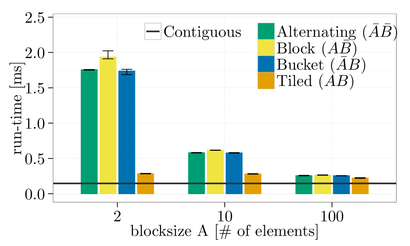
(a) MPI_Allgather

(b) MPI_Bcast

(c) Ping-pong

Figure 32: Contiguous vs. typed, $m=$3.2\text{\,}\mathrm{kB}$$, element datatype: MPI_INT, $32\text{\times}1$ processes ($2\text{\times}1$ for Ping-pong), MVAPICH2-2.1, Variant 2.

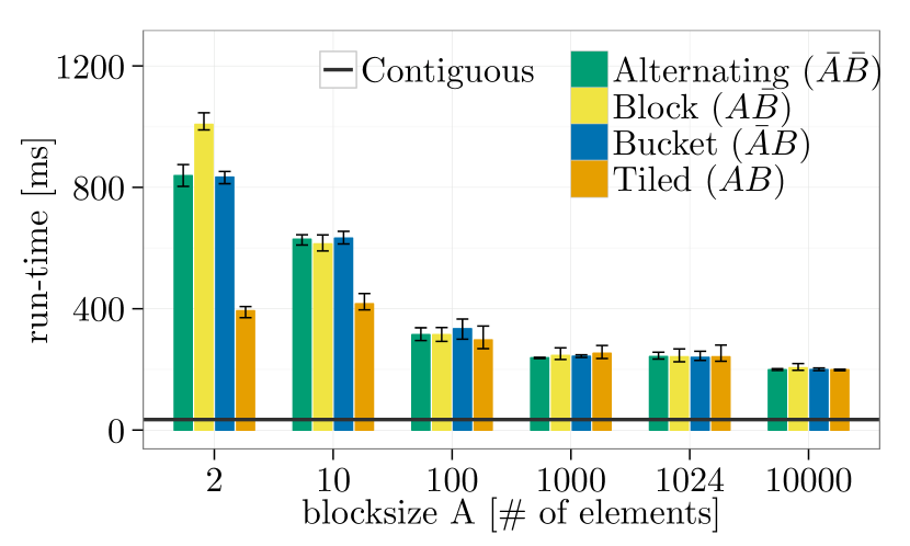
(a) MPI_Allgather

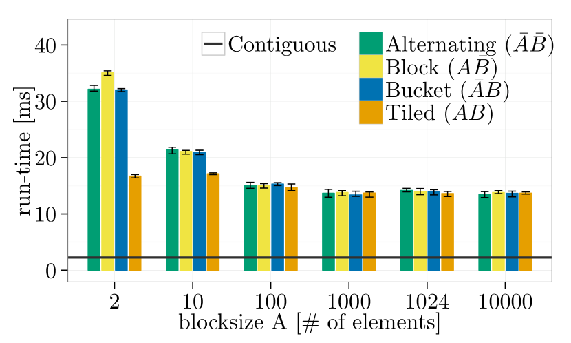
(b) MPI_Bcast

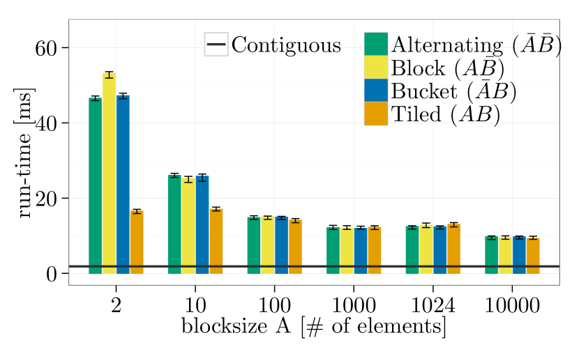
(c) Ping-pong

Figure 33: Contiguous vs. typed, $m=$2.56\text{\,}\mathrm{MB}$$, element datatype: MPI_INT, $32\text{\times}1$ processes ($2\text{\times}1$ for Ping-pong), MVAPICH2-2.1, Variant 2.

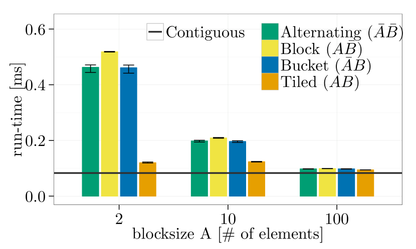
(a) MPI_Allgather

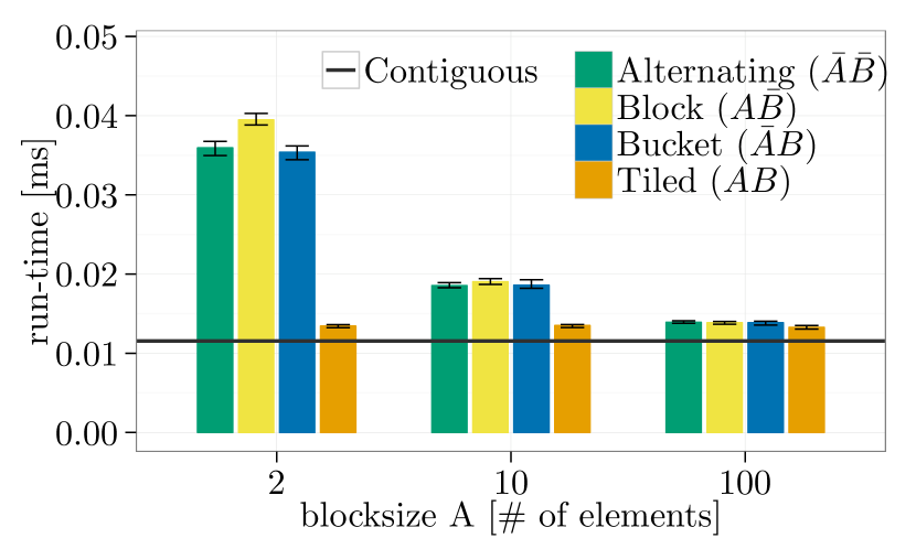
(b) MPI_Bcast

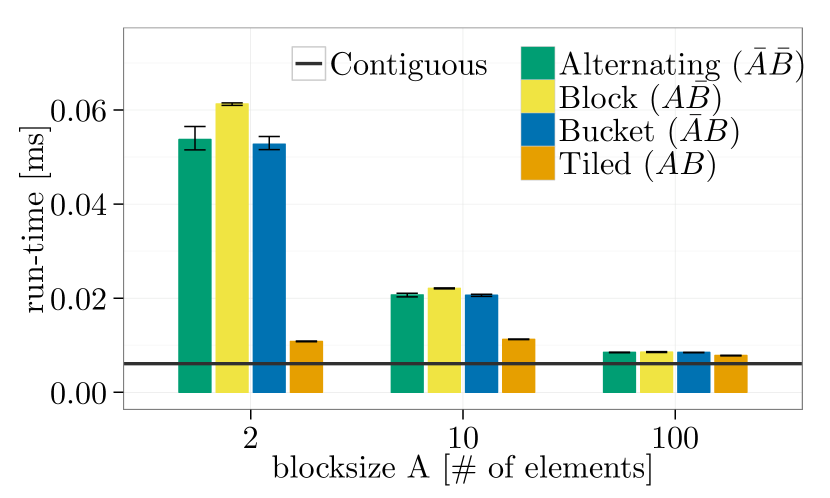
(c) Ping-pong

Figure 34: Contiguous vs. typed, $m=$3.2\text{\,}\mathrm{kB}$$, element datatype: MPI_INT, one node, $16$ processes ($2$ for Ping-pong), MVAPICH2-2.1, Variant 2.

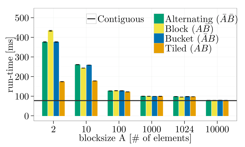
(a) MPI_Allgather

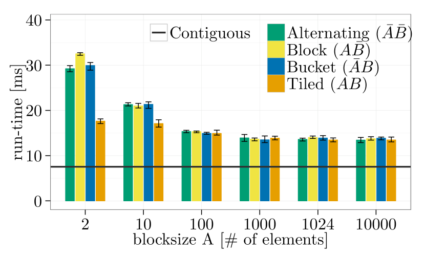
(b) MPI_Bcast

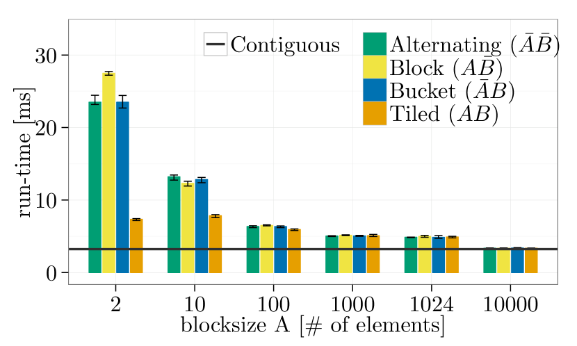
(c) Ping-pong

Figure 35: Contiguous vs. typed, $m=$2.56\text{\,}\mathrm{MB}$$, element datatype: MPI_INT, one node, $16$ processes ($2$ for Ping-pong), MVAPICH2-2.1, Variant 2.

A.2 Expectation Test 2.4.2 (Sect. 2.4.2)

 

• Contiguous, Tiled-heterogeneous ($AB\bar{T}$)

• Ping-pong

 

• Figure 36:   NEC MPI-1.3.1

• Figure 37:   MVAPICH2-2.1

• Figure 38:   OpenMPI-1.10.1

 

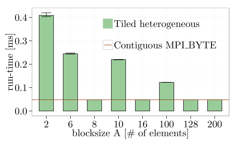
(a) $m=$48\text{\,}\mathrm{kB}$$, $2$ nodes

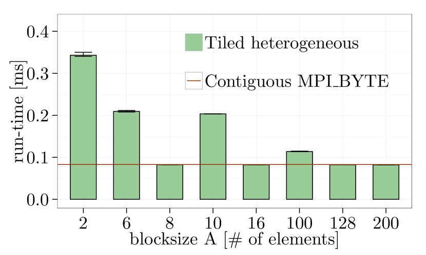
(b) $m=$48\text{\,}\mathrm{kB}$$, same node

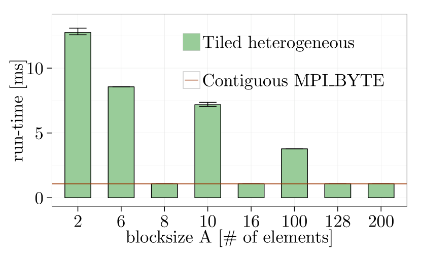
(c) $m=$1.5\text{\,}\mathrm{MB}$$, $2$ nodes

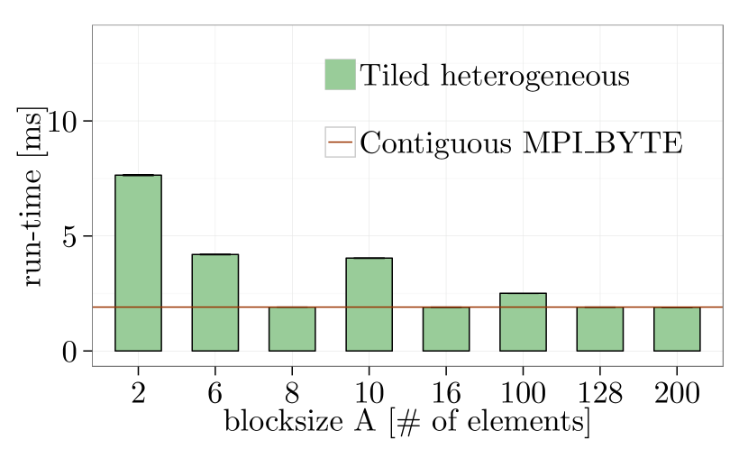
(d) $m=$1.5\text{\,}\mathrm{MB}$$, same node

Figure 36: Contiguous vs. Tiled-heterogeneous ($AB\bar{T}$) $A$=$B$, element datatype: MPI_INT, Ping-pong, NEC MPI-1.3.1.

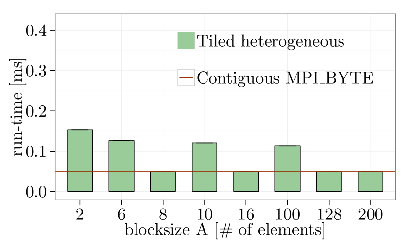
(a) $m=$48\text{\,}\mathrm{kB}$$, $2$ nodes

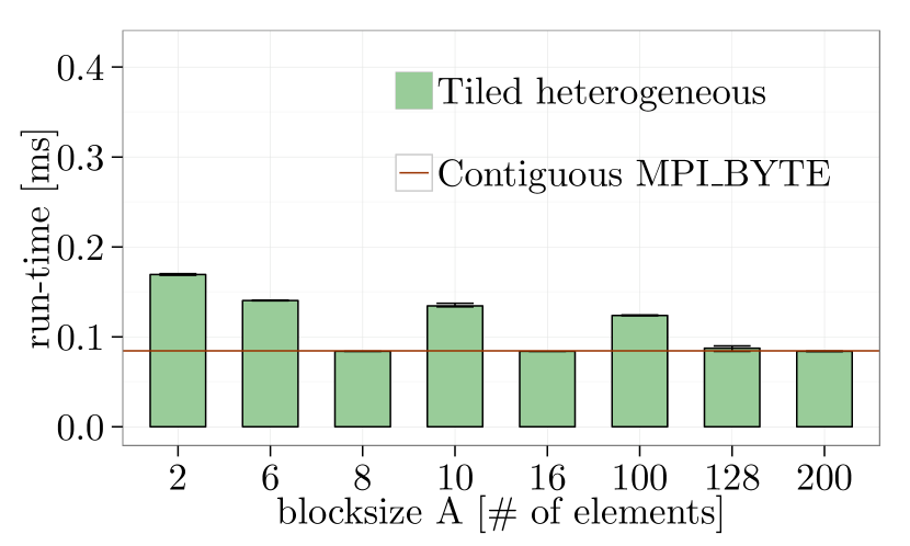
(b) $m=$48\text{\,}\mathrm{kB}$$, same node

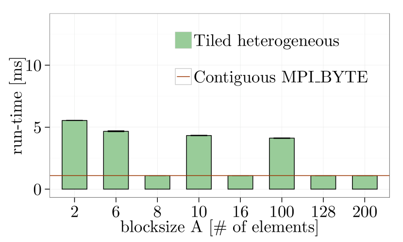
(c) $m=$1.5\text{\,}\mathrm{MB}$$, $2$ nodes

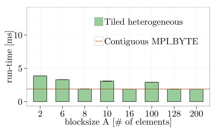
(d) $m=$1.5\text{\,}\mathrm{MB}$$, same node

Figure 37: Contiguous vs. Tiled-heterogeneous ($AB\bar{T}$) $A$=$B$, element datatype: MPI_INT, Ping-pong, MVAPICH2-2.1.

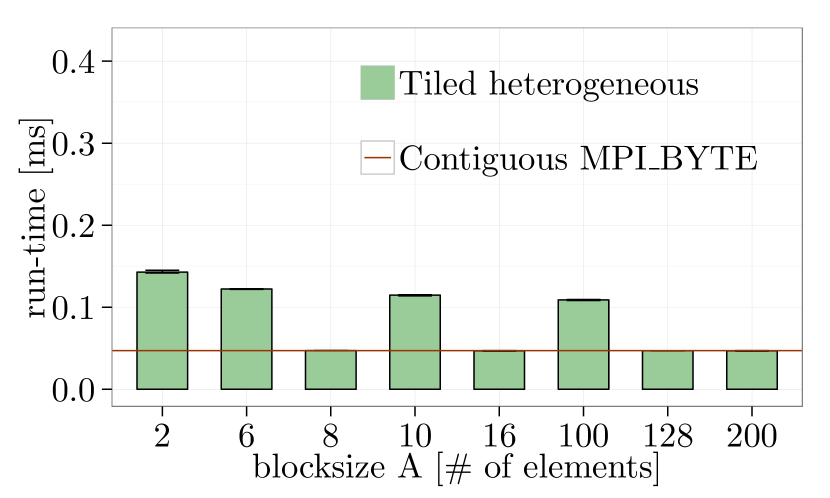
(a) $m=$48\text{\,}\mathrm{kB}$$, $2$ nodes

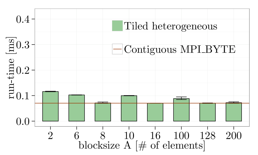
(b) $m=$48\text{\,}\mathrm{kB}$$, same node

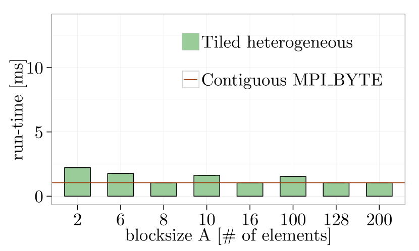
(c) $m=$1.5\text{\,}\mathrm{MB}$$, $2$ nodes

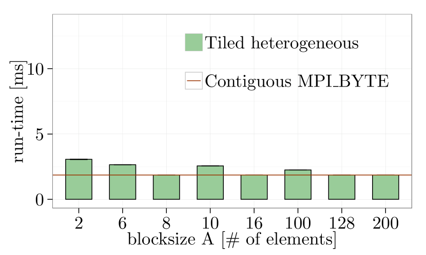
(d) $m=$1.5\text{\,}\mathrm{MB}$$, same node

Figure 38: Contiguous vs. Tiled-heterogeneous ($AB\bar{T}$) $A$=$B$, element datatype: MPI_INT, Ping-pong, OpenMPI-1.10.1.

A.3 Expectation Test 3.2.1 (Sect. 3.2.1)

 

• pack vs. unpack for basic layouts (Tiled, Block, Bucket, Alternating)

• MPI_Allgather, MPI_Bcast, Ping-pong

 

• Figure 39:   NEC MPI-1.3.1, Ping-pong, $2\text{\times}1$ processes

• Figure 40:   MVAPICH2-2.1, Ping-pong, $2\text{\times}1$ processes

• Figure 41:   OpenMPI-1.10.1, Ping-pong, $2\text{\times}1$ processes

• Figure 42:   NEC MPI-1.3.1, MPI_Allgather, $32\text{\times}1$ processes

• Figure 43:   MVAPICH2-2.1, MPI_Allgather, $32\text{\times}1$ processes

• Figure 44:   OpenMPI-1.10.1, MPI_Allgather, $32\text{\times}1$ processes

• Figure 45:   NEC MPI-1.3.1, MPI_Bcast, $32\text{\times}1$ processes

• Figure 46:   MVAPICH2-2.1, MPI_Bcast, $32\text{\times}1$ processes

• Figure 47:   OpenMPI-1.10.1, MPI_Bcast, $32\text{\times}1$ processes

• Figure 48:   NEC MPI-1.3.1, Ping-pong, one node, $2$ processes

• Figure 49:   MVAPICH2-2.1, Ping-pong, one node, $2$ processes

• Figure 50:   OpenMPI-1.10.1, Ping-pong, one node, $2$ processes

• Figure 51:   NEC MPI-1.3.1, MPI_Allgather, one node, $16$ processes

• Figure 52:   MVAPICH2-2.1, MPI_Allgather, one node, $16$ processes

• Figure 53:   OpenMPI-1.10.1, MPI_Allgather, one node, $16$ processes

• Figure 54:   NEC MPI-1.3.1, MPI_Bcast, one node, $16$ processes

• Figure 55:   MVAPICH2-2.1, MPI_Bcast, one node, $16$ processes

• Figure 56:   OpenMPI-1.10.1, MPI_Bcast, one node, $16$ processes

 

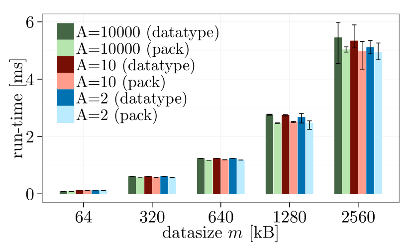
(a) Tiled

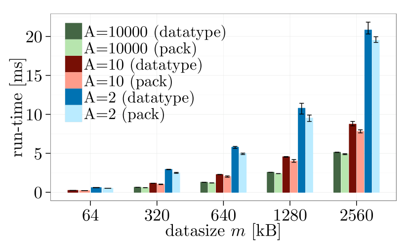
(b) Block

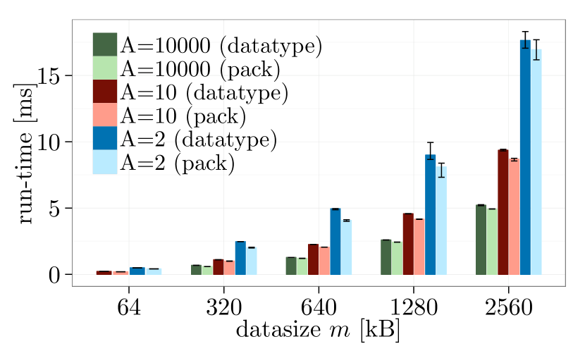
(c) Bucket

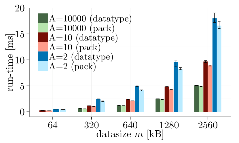
(d) Alternating

Figure 39: Basic layouts vs. pack/unpack, element datatype: MPI_INT, $2\text{\times}1$ processes, Ping-pong, NEC MPI-1.3.1.

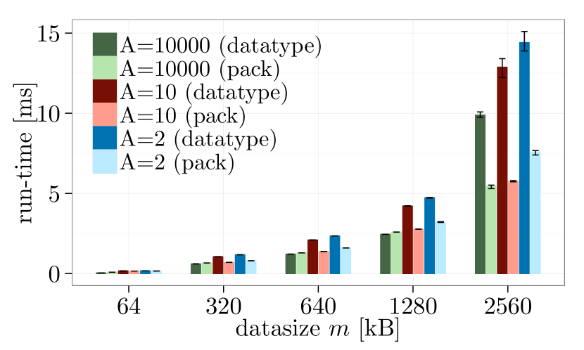
(a) Tiled

(b) Block

(c) Bucket

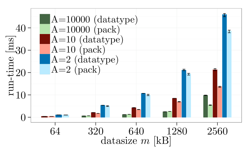
(d) Alternating

Figure 40: Basic layouts vs. pack/unpack, element datatype: MPI_INT, $2\text{\times}1$ processes, Ping-pong, MVAPICH2-2.1.

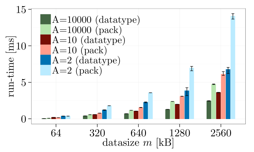
(a) Tiled

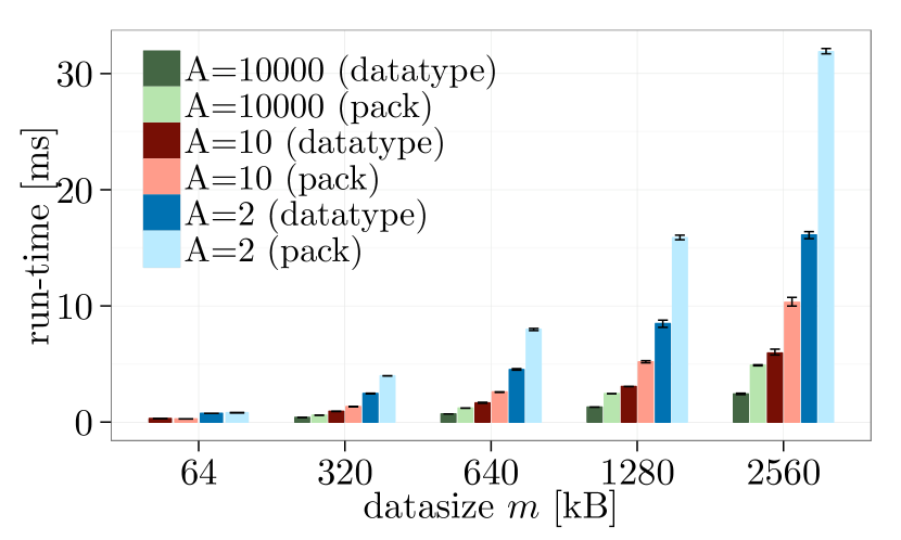
(b) Block

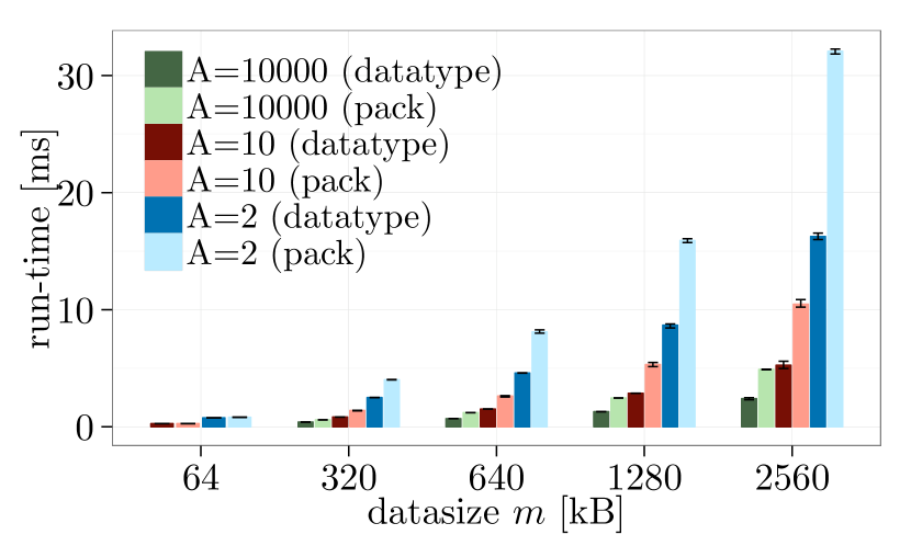
(c) Bucket

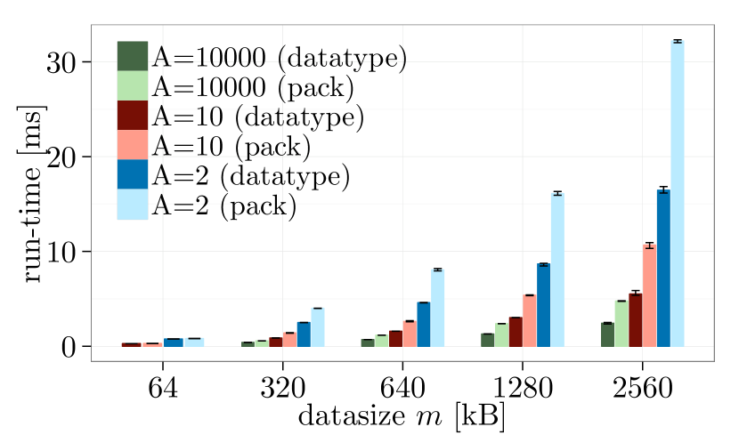
(d) Alternating

Figure 41: Basic layouts vs. pack/unpack, element datatype: MPI_INT, $2\text{\times}1$ processes, Ping-pong, OpenMPI-1.10.1.

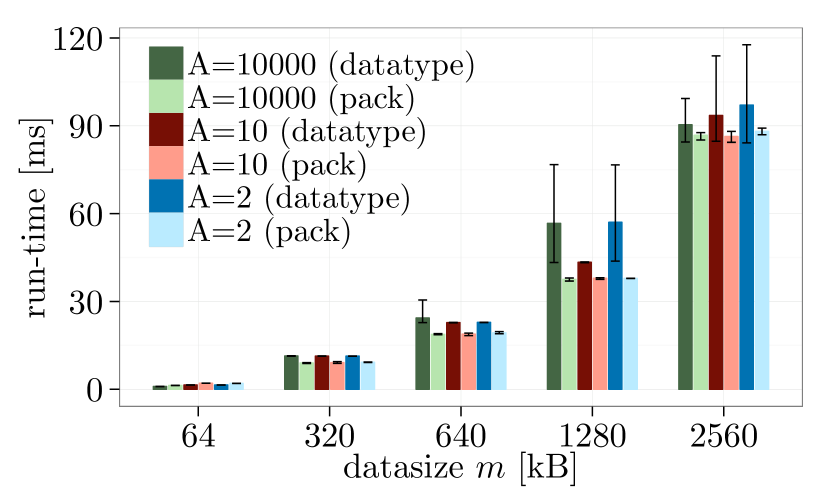
(a) Tiled

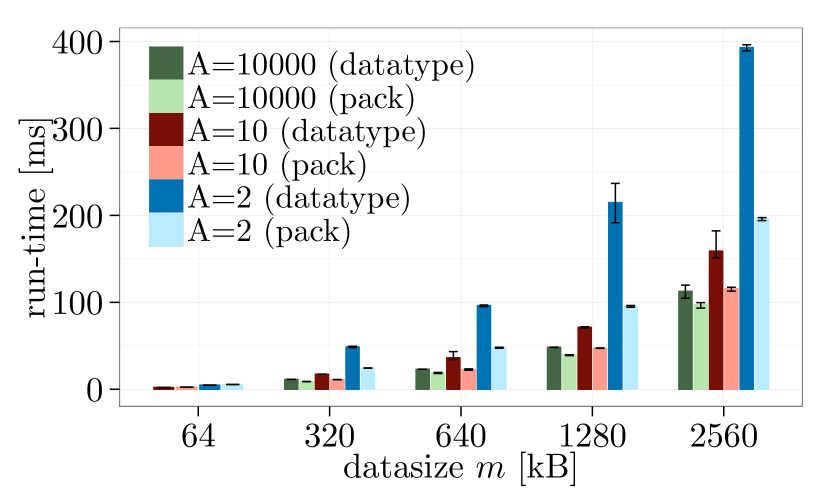
(b) Block

(c) Bucket

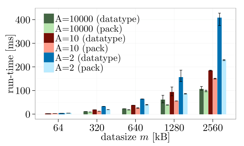
(d) Alternating

Figure 42: Basic layouts vs. pack/unpack, element datatype: MPI_INT, $32\text{\times}1$ processes, MPI_Allgather, NEC MPI-1.3.1.

(a) Tiled

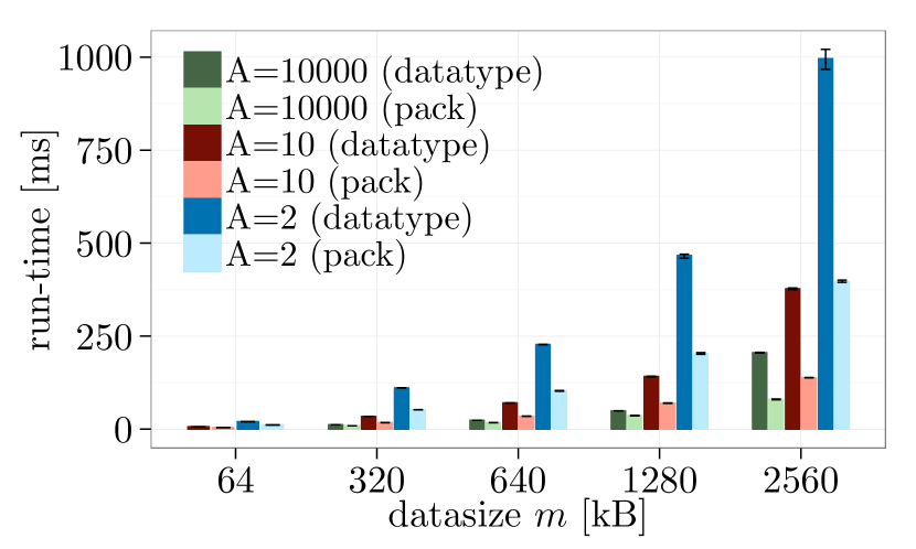
(b) Block

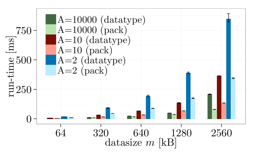
(c) Bucket

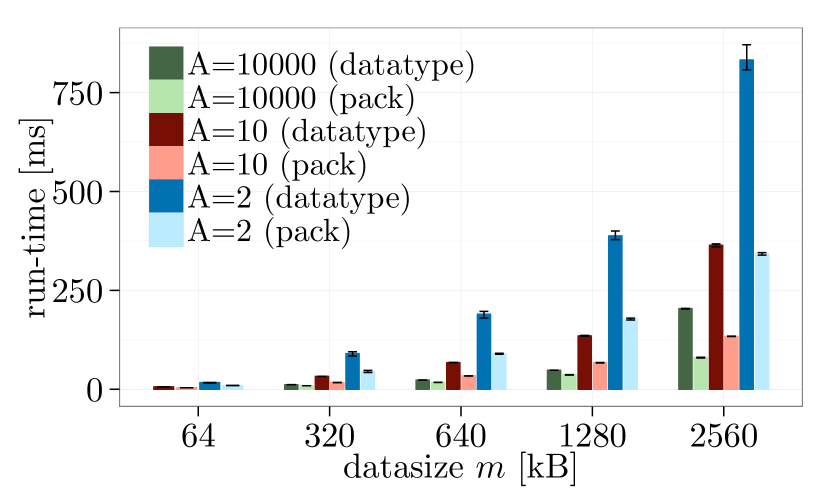
(d) Alternating

Figure 43: Basic layouts vs. pack/unpack, element datatype: MPI_INT, $32\text{\times}1$ processes, MPI_Allgather, MVAPICH2-2.1.

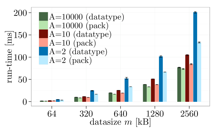
(a) Tiled

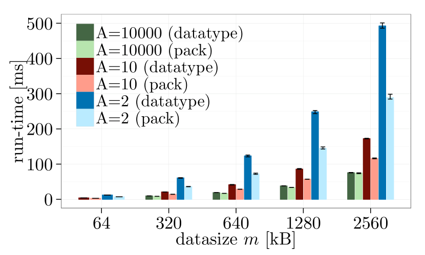
(b) Block

(c) Bucket

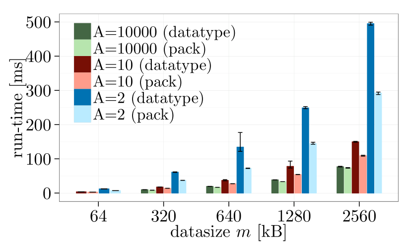
(d) Alternating

Figure 44: Basic layouts vs. pack/unpack, element datatype: MPI_INT, $32\text{\times}1$ processes, MPI_Allgather, OpenMPI-1.10.1.

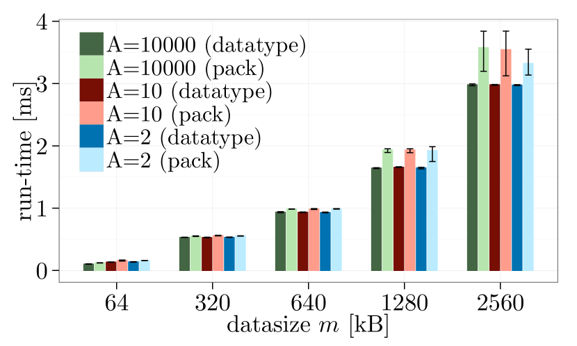
(a) Tiled

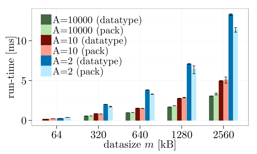
(b) Block

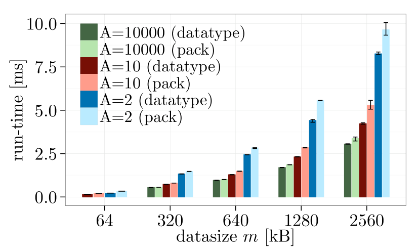
(c) Bucket

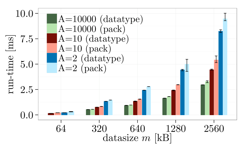
(d) Alternating

Figure 45: Basic layouts vs. pack/unpack, element datatype: MPI_INT, $32\text{\times}1$ processes, MPI_Bcast, NEC MPI-1.3.1.

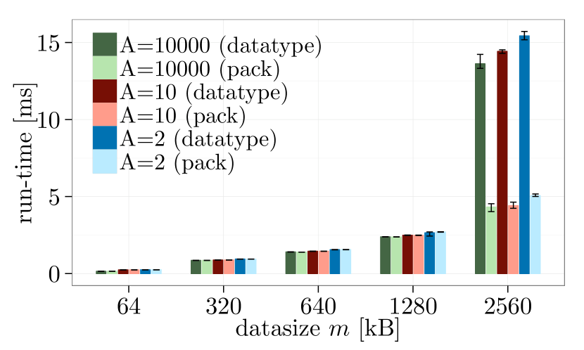
(a) Tiled

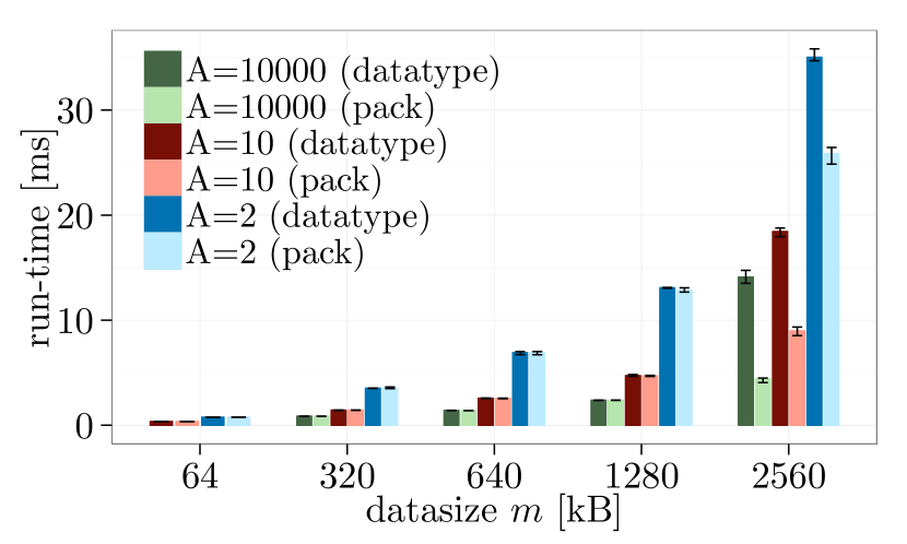
(b) Block

(c) Bucket

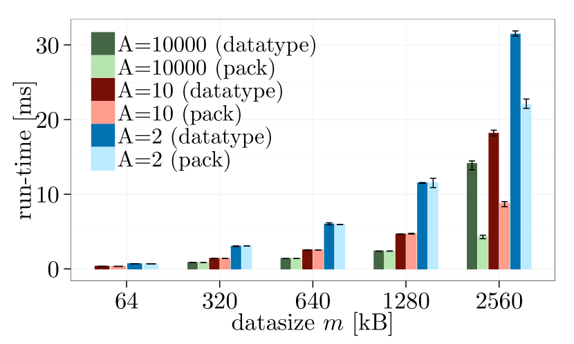
(d) Alternating

Figure 46: Basic layouts vs. pack/unpack, element datatype: MPI_INT, $32\text{\times}1$ processes, MPI_Bcast, MVAPICH2-2.1.

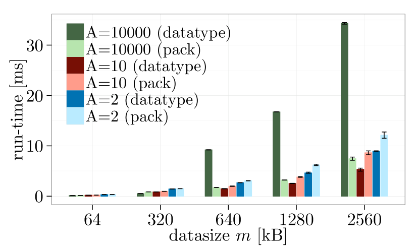
(a) Tiled

(b) Block

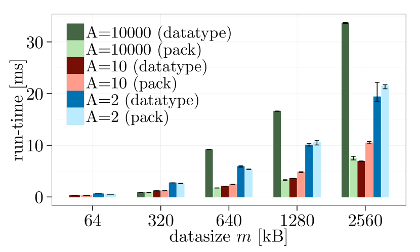
(c) Bucket

(d) Alternating

Figure 47: Basic layouts vs. pack/unpack, element datatype: MPI_INT, $32\text{\times}1$ processes, MPI_Bcast, OpenMPI-1.10.1.

(a) Tiled

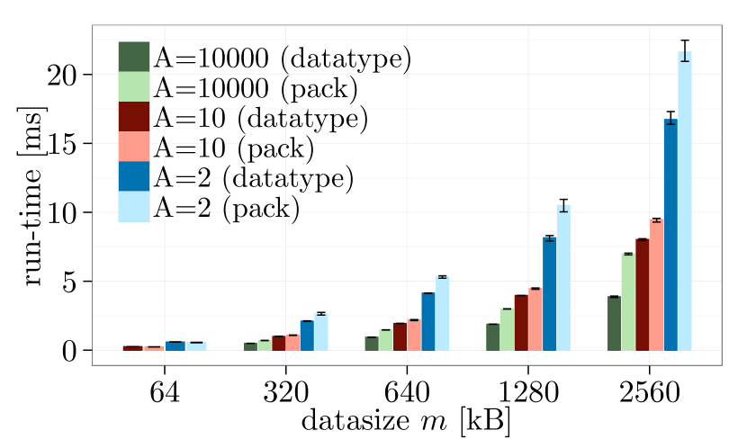
(b) Block

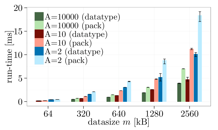
(c) Bucket

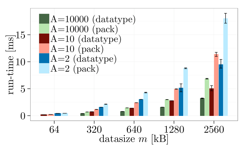
(d) Alternating

Figure 48: Basic layouts vs. pack/unpack, element datatype: MPI_INT, one node, $2$ processes, Ping-pong, NEC MPI-1.3.1.

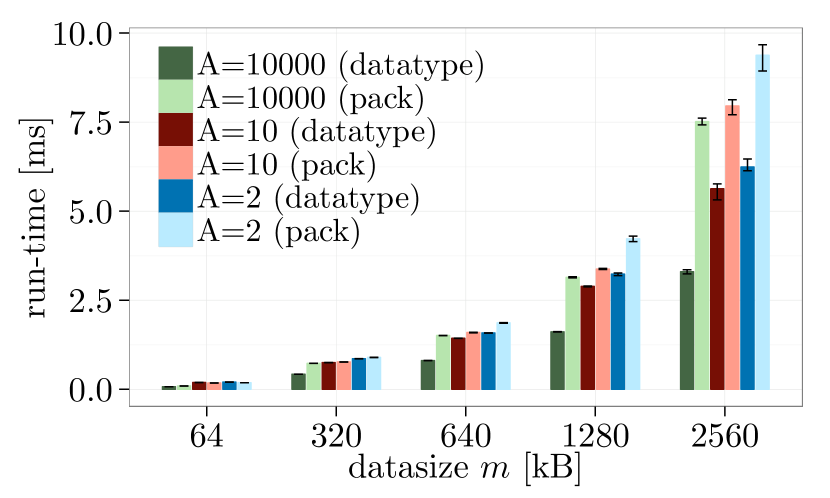
(a) Tiled

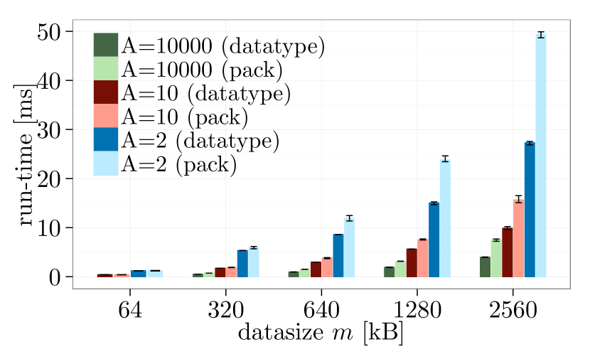
(b) Block

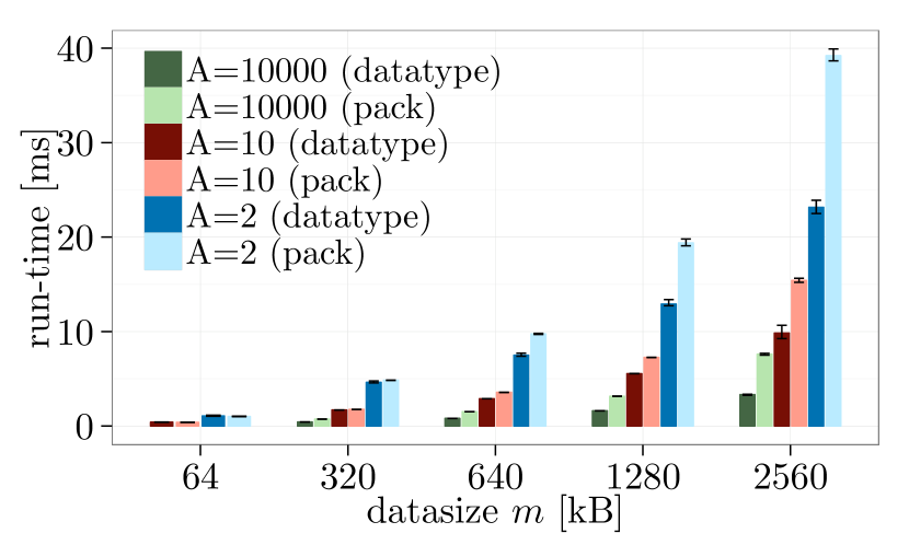
(c) Bucket

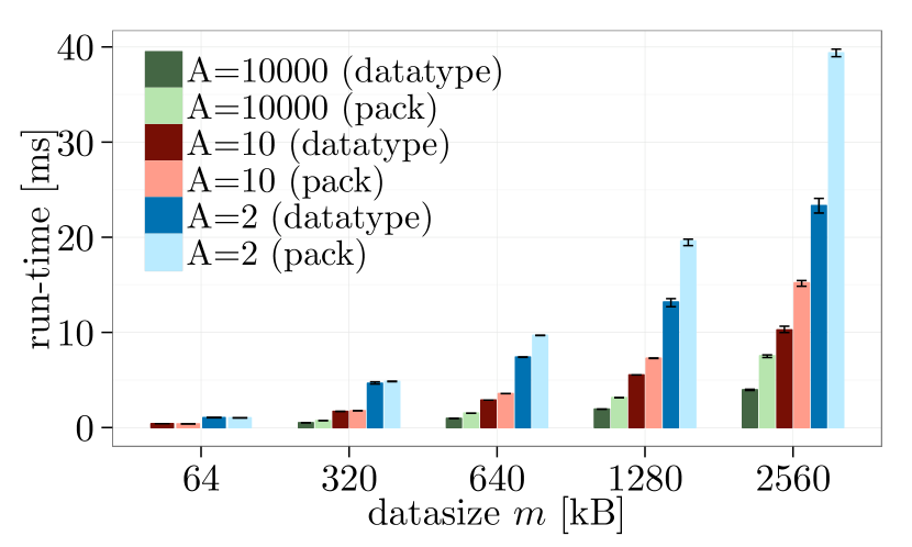
(d) Alternating

Figure 49: Basic layouts vs. pack/unpack, element datatype: MPI_INT, one node, $2$ processes, Ping-pong, MVAPICH2-2.1.

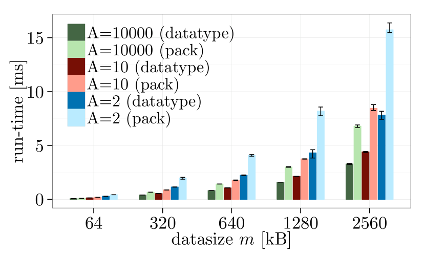
(a) Tiled

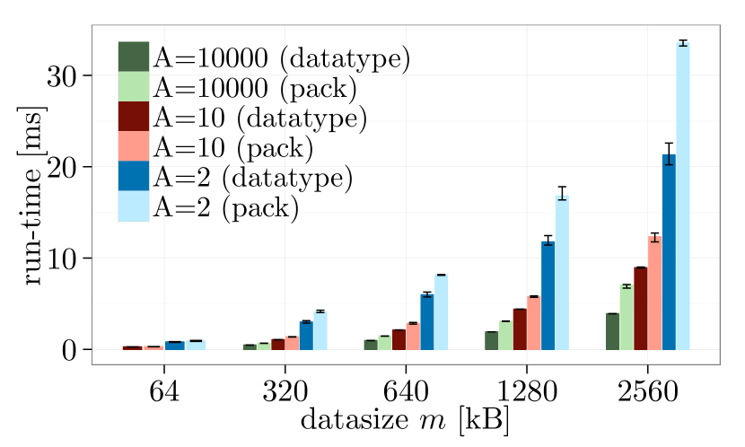
(b) Block

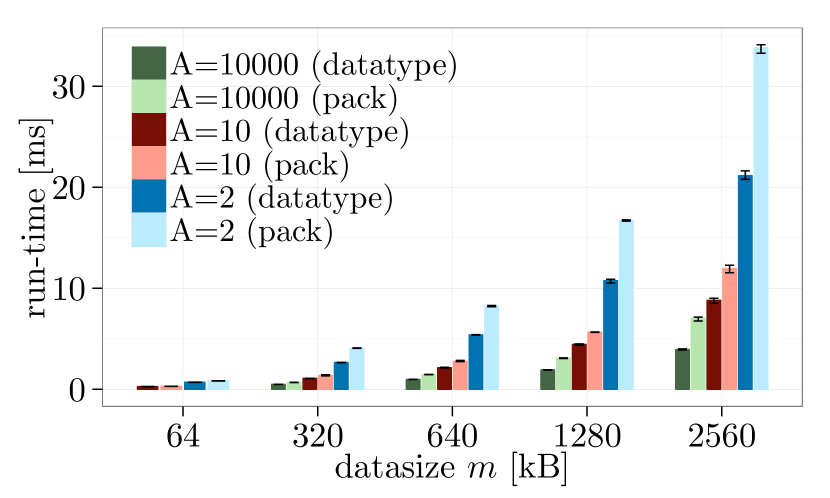
(c) Bucket

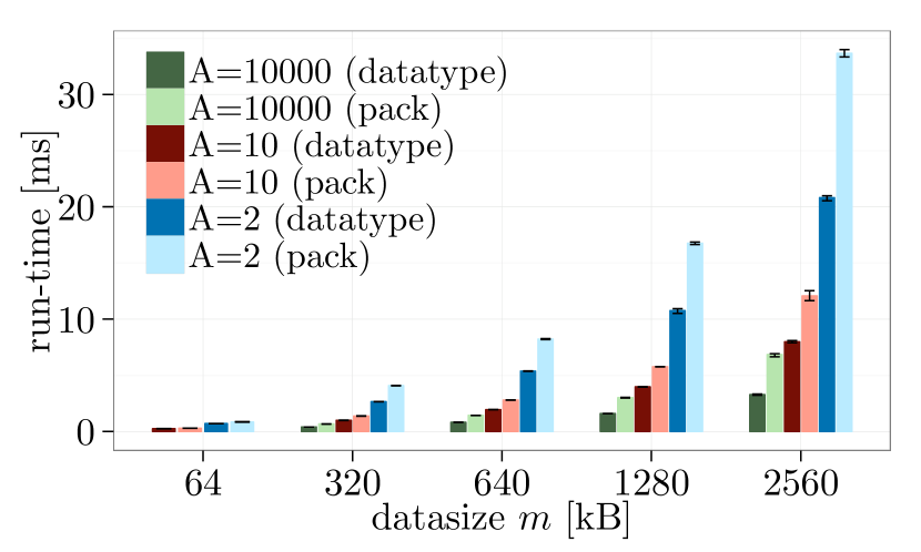
(d) Alternating

Figure 50: Basic layouts vs. pack/unpack, element datatype: MPI_INT, one node, $2$ processes, Ping-pong, OpenMPI-1.10.1.

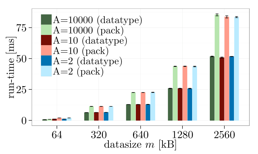
(a) Tiled

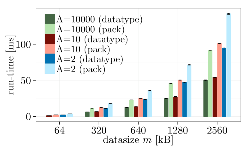
(b) Block

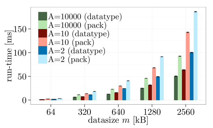
(c) Bucket

(d) Alternating

Figure 51: Basic layouts vs. pack/unpack, element datatype: MPI_INT, one node, $16$ processes, MPI_Allgather, NEC MPI-1.3.1.

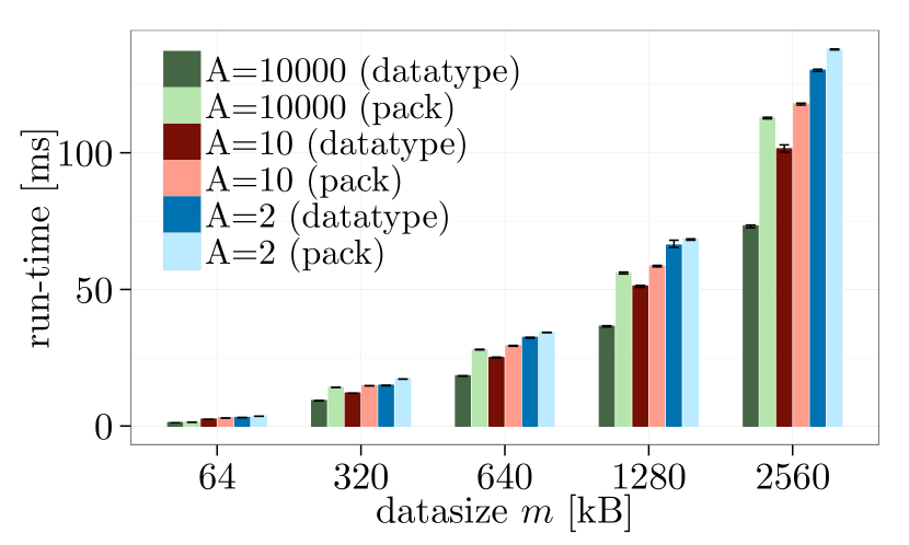
(a) Tiled

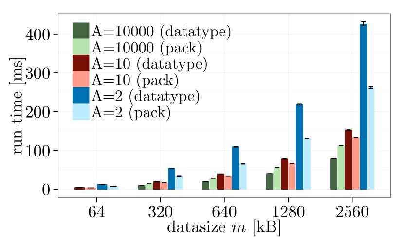
(b) Block

(c) Bucket

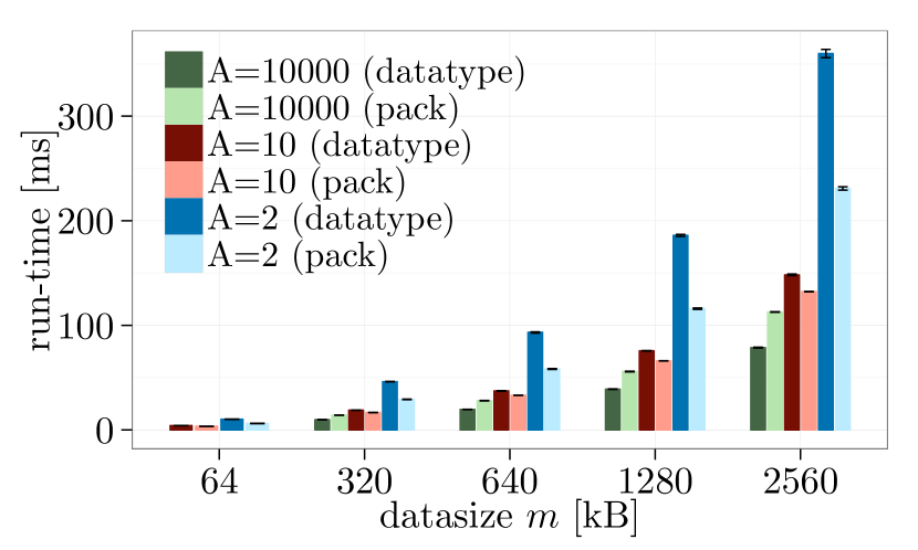
(d) Alternating

Figure 52: Basic layouts vs. pack/unpack, element datatype: MPI_INT, one node, $16$ processes, MPI_Allgather, MVAPICH2-2.1.

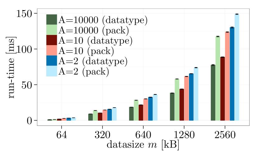
(a) Tiled

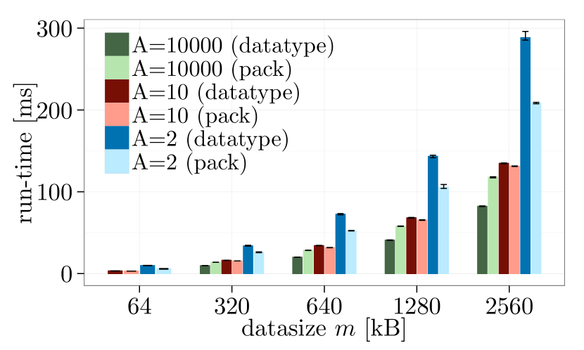
(b) Block

(c) Bucket

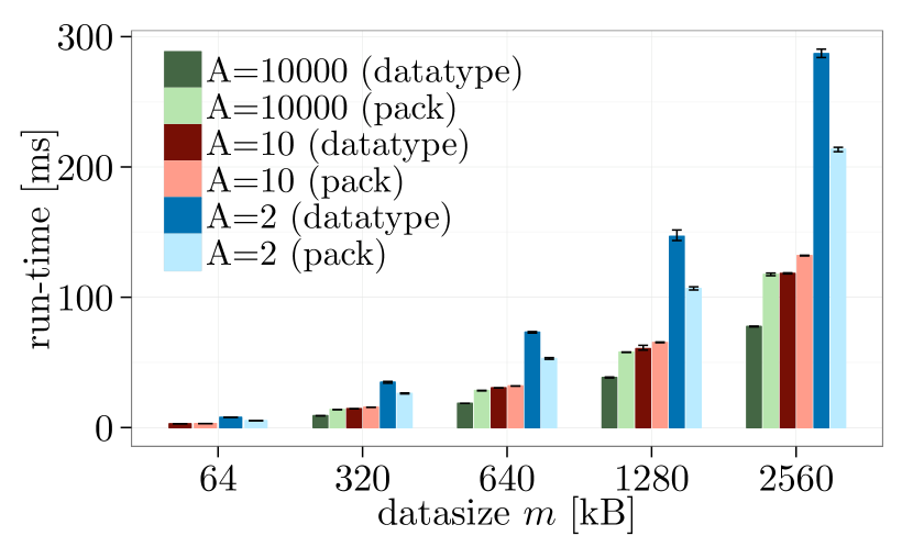
(d) Alternating

Figure 53: Basic layouts vs. pack/unpack, element datatype: MPI_INT, one node, $16$ processes, MPI_Allgather, OpenMPI-1.10.1.

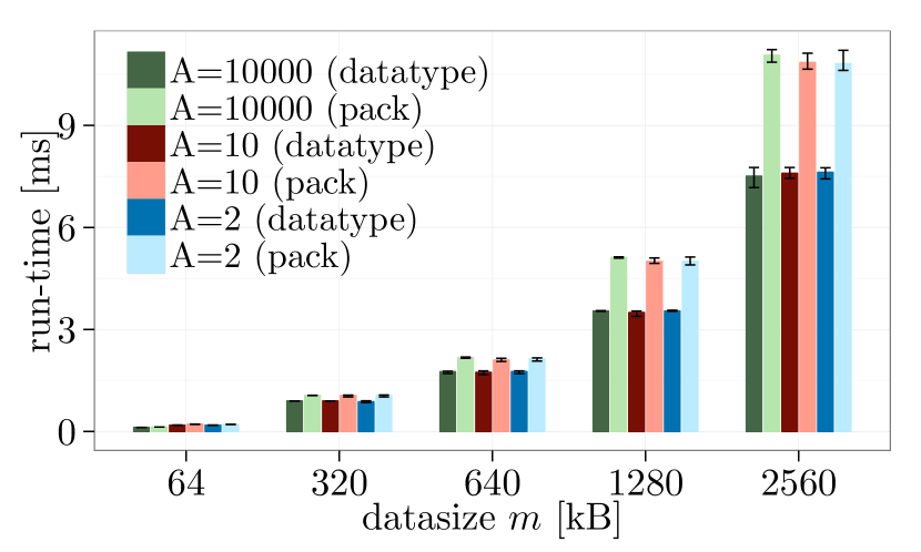
(a) Tiled

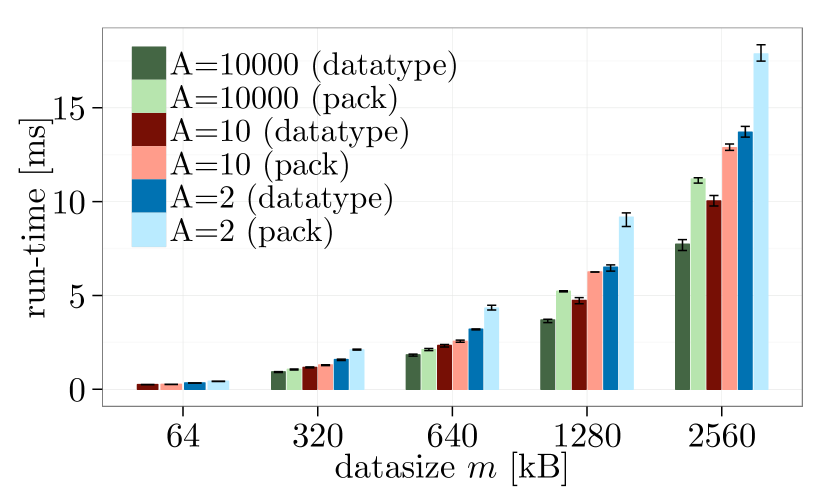
(b) Block

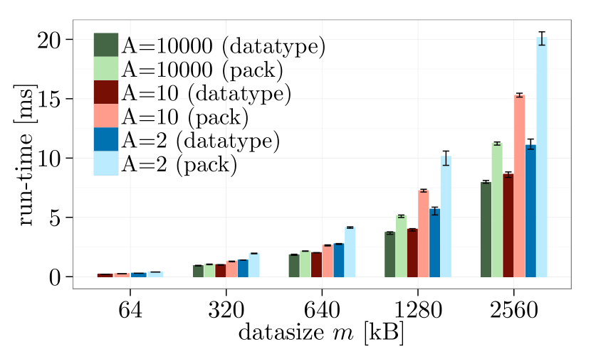
(c) Bucket

(d) Alternating

Figure 54: Basic layouts vs. pack/unpack, element datatype: MPI_INT, one node, $16$ processes, MPI_Bcast, NEC MPI-1.3.1.

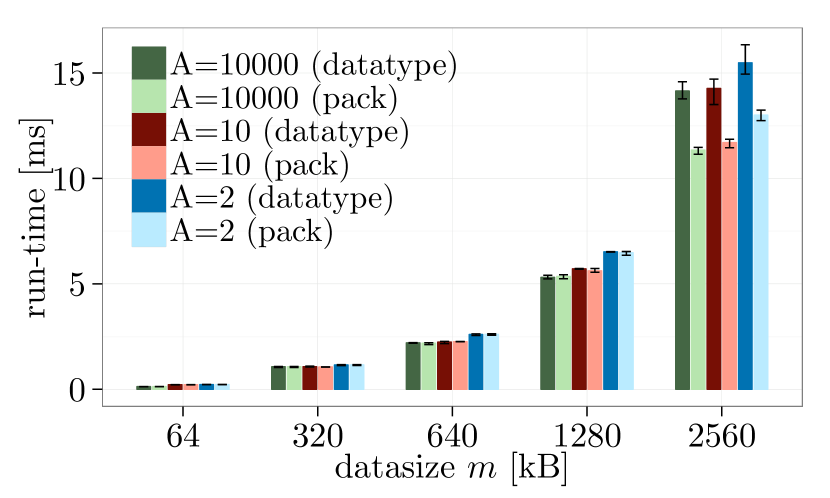
(a) Tiled

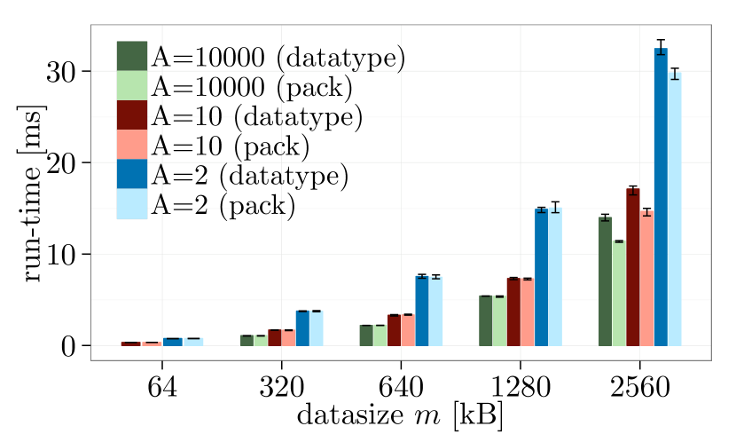
(b) Block

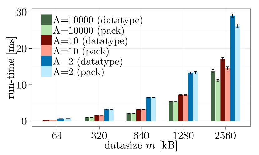
(c) Bucket

(d) Alternating

Figure 55: Basic layouts vs. pack/unpack, element datatype: MPI_INT, one node, $16$ processes, MPI_Bcast, MVAPICH2-2.1.

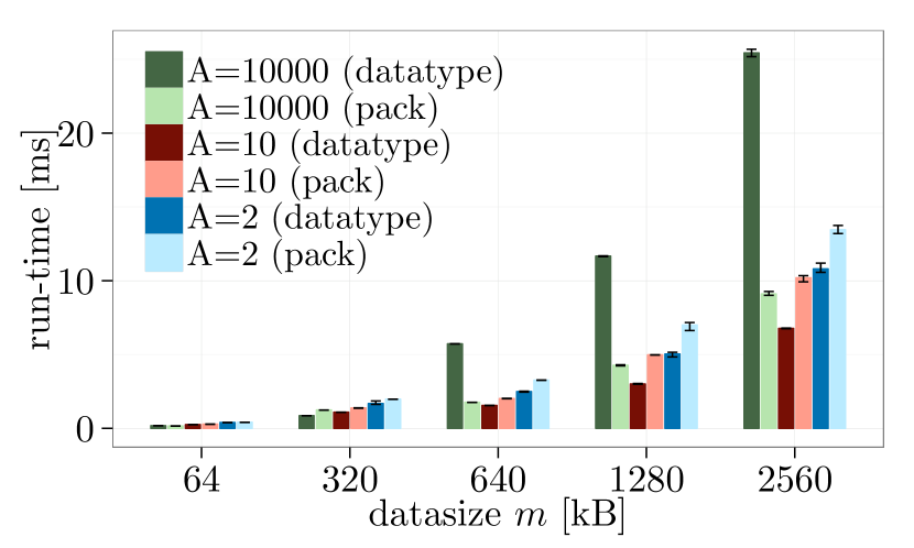
(a) Tiled

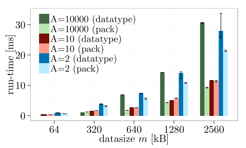
(b) Block

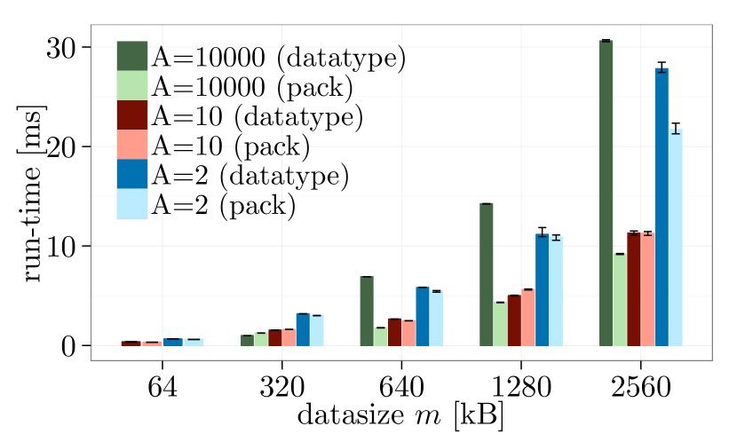
(c) Bucket

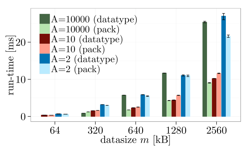
(d) Alternating

Figure 56: Basic layouts vs. pack/unpack, element datatype: MPI_INT, one node, $16$ processes, MPI_Bcast, OpenMPI-1.10.1.

A.4 Expectation Test 3.2.2 (Sect. 3.2.2)

 

• Contiguous-subtype vs. basic layouts (Tiled, Block, Bucket, Alternating)

• Ping-pong

 

• Figure 57:   NEC MPI-1.3.1, small datasize

• Figure 58:   MVAPICH2-2.1, small datasize

• Figure 59:   OpenMPI-1.10.1, small datasize

• Figure 60:   NEC MPI-1.3.1, large datasize

• Figure 61:   MVAPICH2-2.1, large datasize

• Figure 62:   OpenMPI-1.10.1, large datasize

 

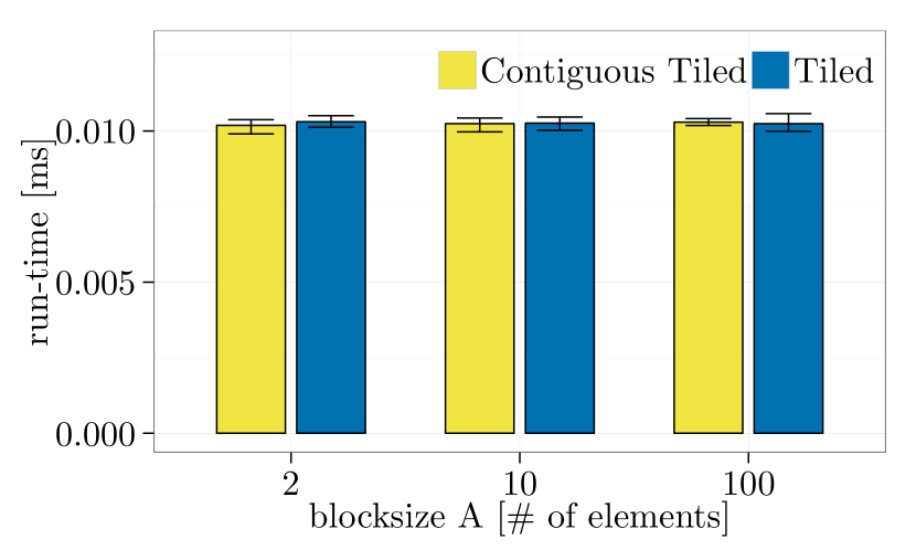
(a) Tiled

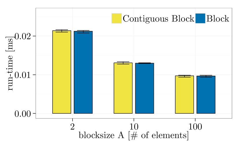
(b) Block

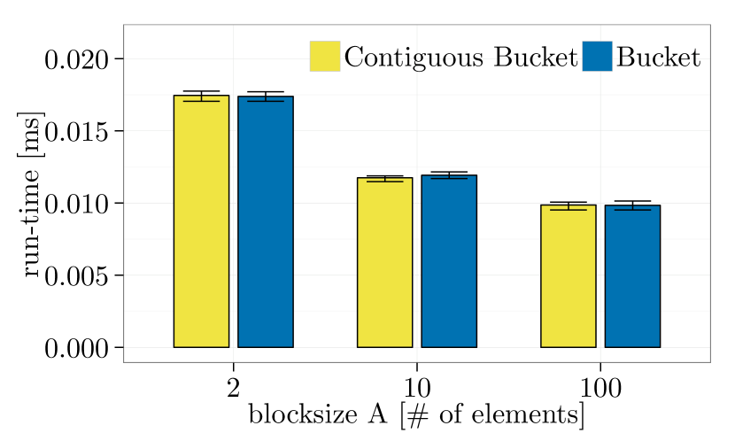
(c) Bucket

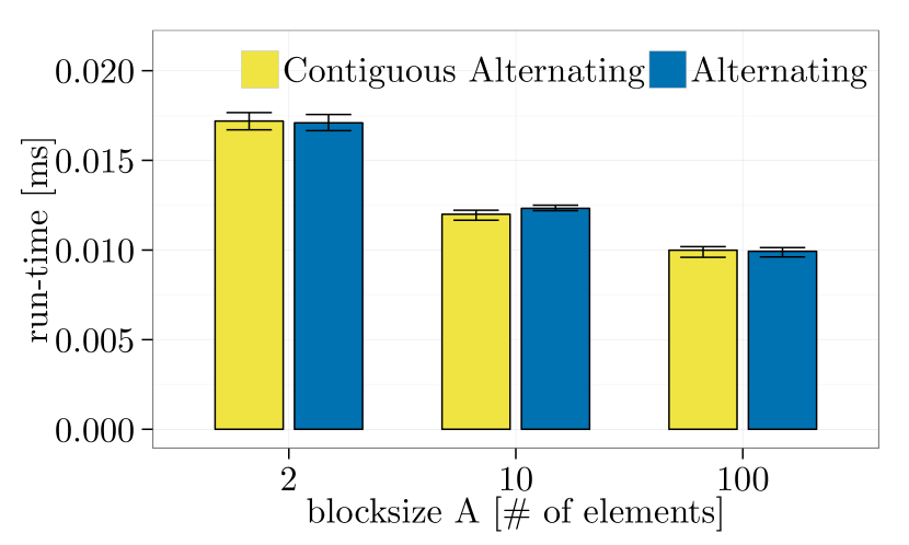
(d) Alternating

Figure 57: Basic layouts vs. Contiguous-subtype, $m=$2\text{\,}\mathrm{kB}$$, element datatype: MPI_INT, $2\text{\times}1$ processes, Ping-pong, NEC MPI-1.3.1 (similar results for $1\text{\times}2$ processes).

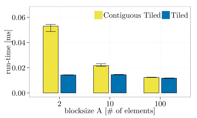
(a) Tiled

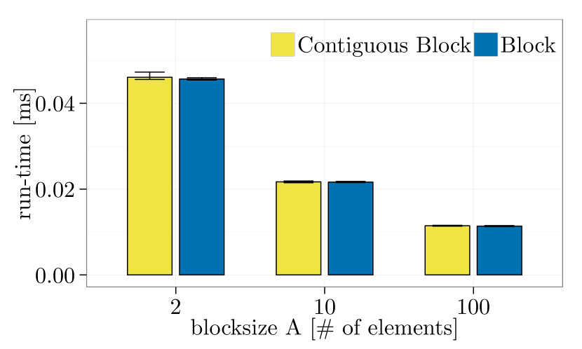
(b) Block

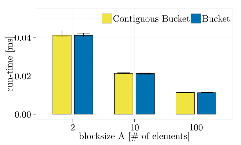
(c) Bucket

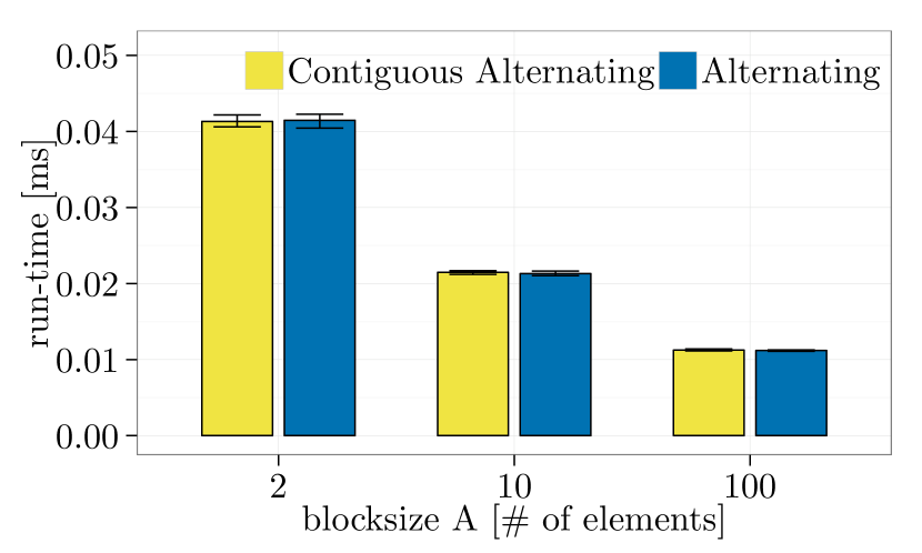
(d) Alternating

Figure 58: Basic layouts vs. Contiguous-subtype, $m=$2\text{\,}\mathrm{kB}$$, element datatype: MPI_INT, $2\text{\times}1$ processes, Ping-pong, MVAPICH2-2.1 (similar results for $1\text{\times}2$ processes).

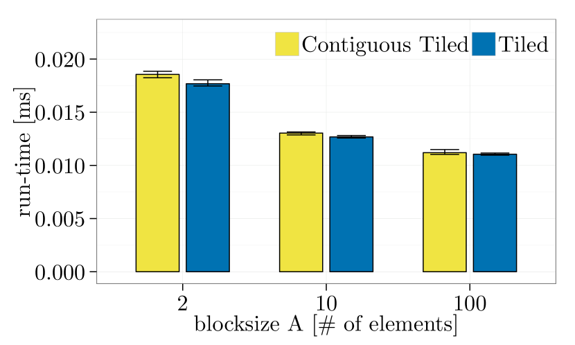
(a) Tiled

(b) Block

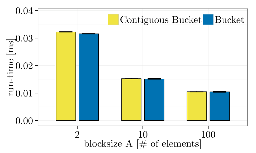
(c) Bucket

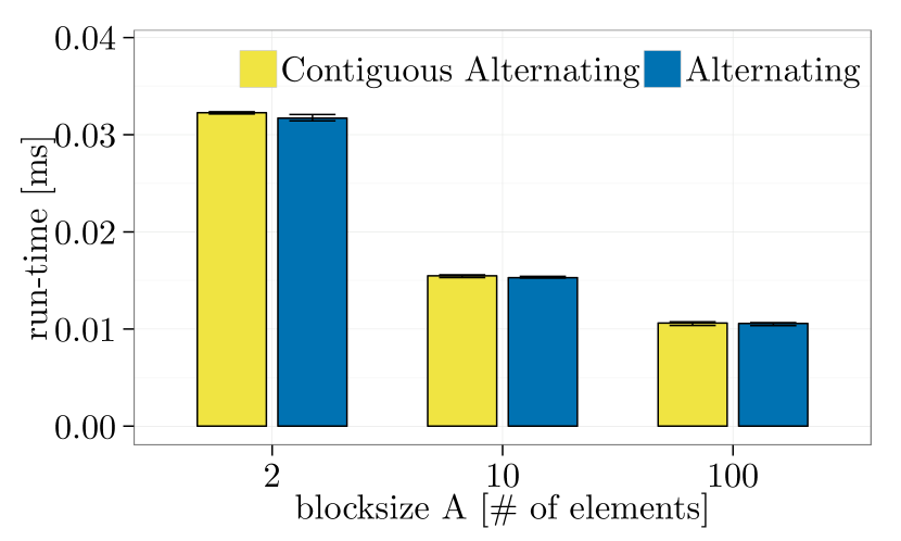
(d) Alternating

Figure 59: Basic layouts vs. Contiguous-subtype, $m=$2\text{\,}\mathrm{kB}$$, element datatype: MPI_INT, $2\text{\times}1$ processes, Ping-pong, OpenMPI-1.10.1 (similar results for $1\text{\times}2$ processes).

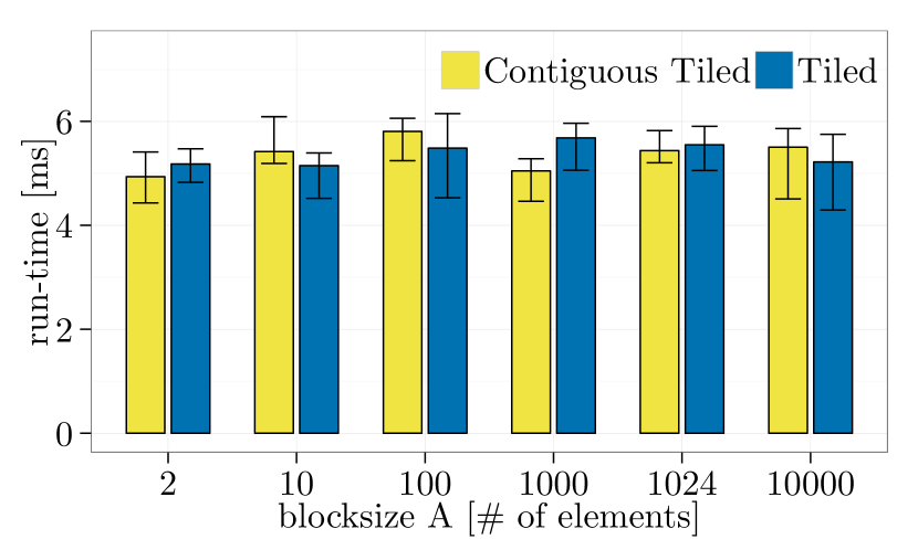
(a) Tiled

(b) Block

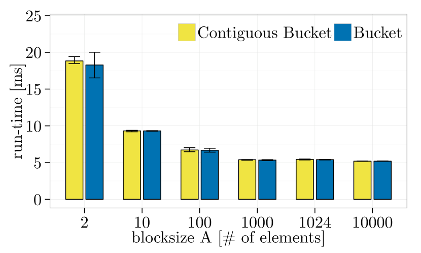
(c) Bucket

(d) Alternating

Figure 60: Basic layouts vs. Contiguous-subtype, $m=$2.56\text{\,}\mathrm{MB}$$, element datatype: MPI_INT, $2\text{\times}1$ processes, Ping-pong, NEC MPI-1.3.1 (similar results for $1\text{\times}2$ processes).

(a) Tiled

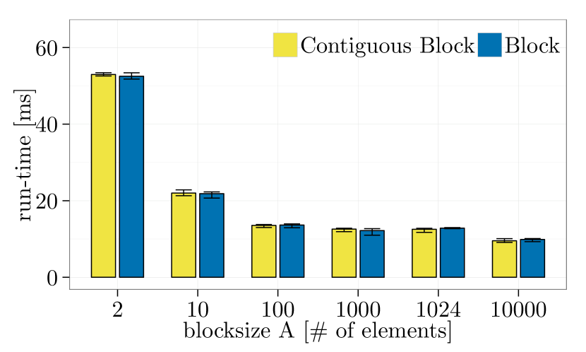
(b) Block

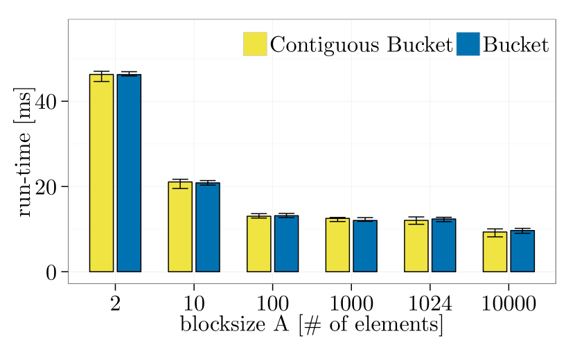
(c) Bucket

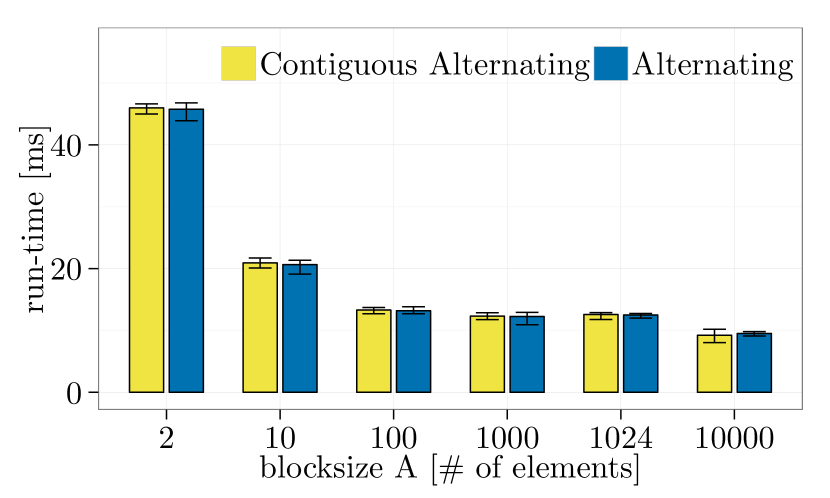
(d) Alternating

Figure 61: Basic layouts vs. Contiguous-subtype, $m=$2.56\text{\,}\mathrm{MB}$$, element datatype: MPI_INT, $2\text{\times}1$ processes, Ping-pong, MVAPICH2-2.1 (similar results for $1\text{\times}2$ processes).

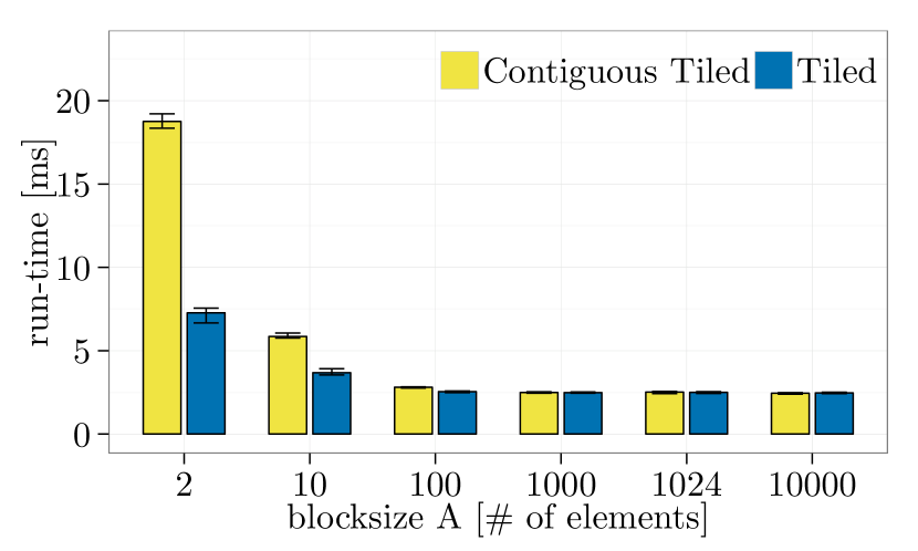
(a) Tiled

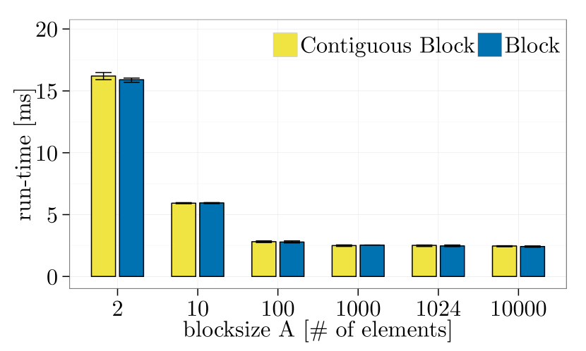
(b) Block

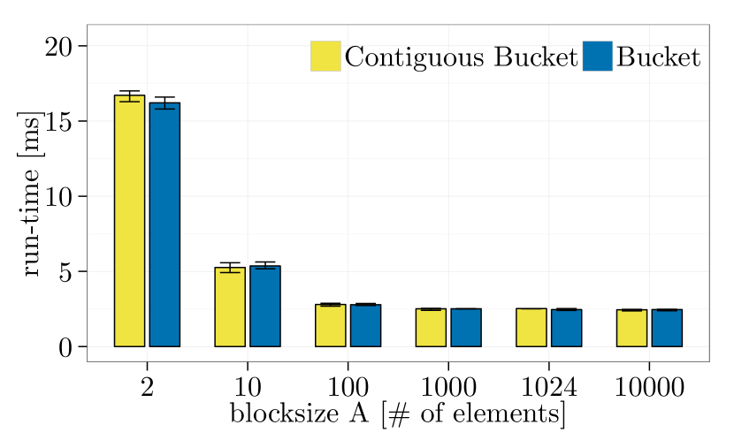
(c) Bucket

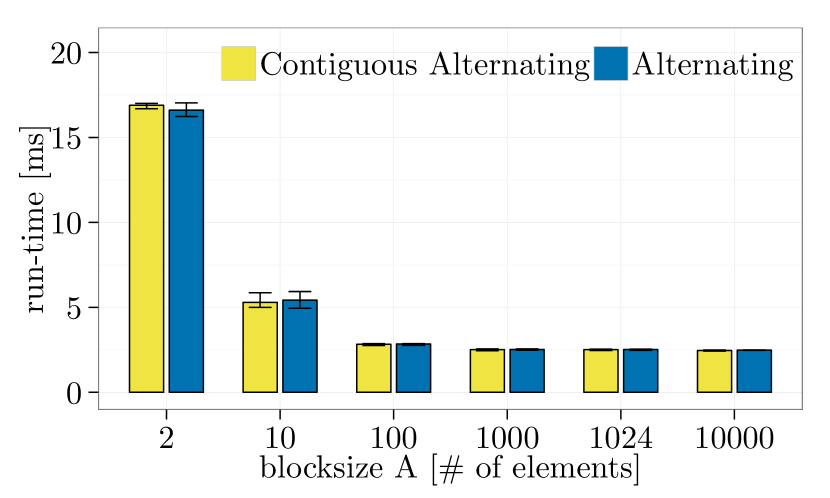
(d) Alternating

Figure 62: Basic layouts vs. Contiguous-subtype, $m=$2.56\text{\,}\mathrm{MB}$$, element datatype: MPI_INT, $2\text{\times}1$ processes, Ping-pong, OpenMPI-1.10.1 (similar results for $1\text{\times}2$ processes).

A.5 Expectation Test 3.2.3 (Sect. 3.2.3)

 

• Tiled ($AB$), Tiled-struct

• Ping-pong

 

• Figure 63:   NEC MPI-1.3.1

• Figure 64:   MVAPICH2-2.1

• Figure 65:   OpenMPI-1.10.1

 

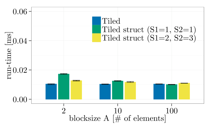
(a) $m=$2\text{\,}\mathrm{kB}$$, $2$ nodes

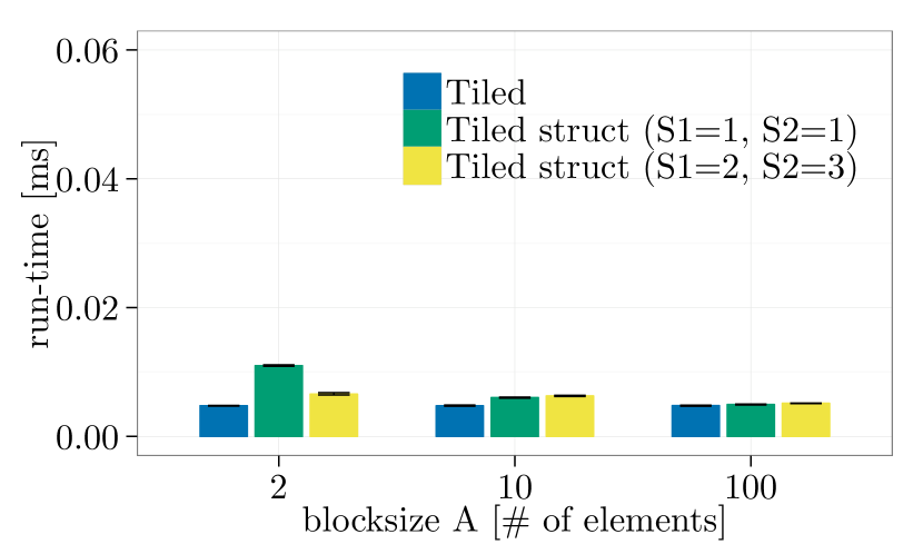
(b) $m=$2\text{\,}\mathrm{kB}$$, same node

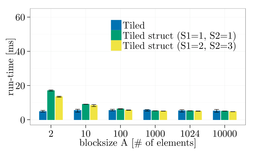
(c) $m=$2.56\text{\,}\mathrm{MB}$$, $2$ nodes

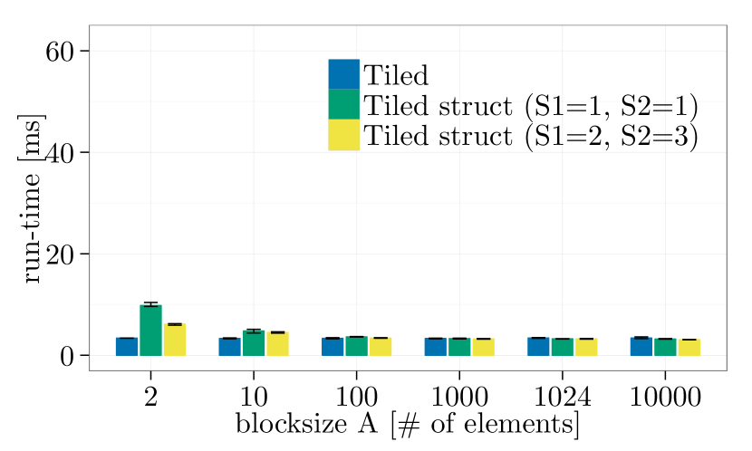
(d) $m=$2.56\text{\,}\mathrm{MB}$$, same node

Figure 63: Tiled ($AB$) vs. Tiled-struct, element datatype: MPI_INT, Ping-pong, NEC MPI-1.3.1.

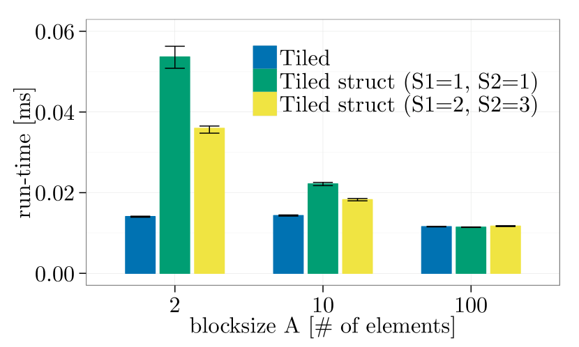
(a) $m=$2\text{\,}\mathrm{kB}$$, $2$ nodes

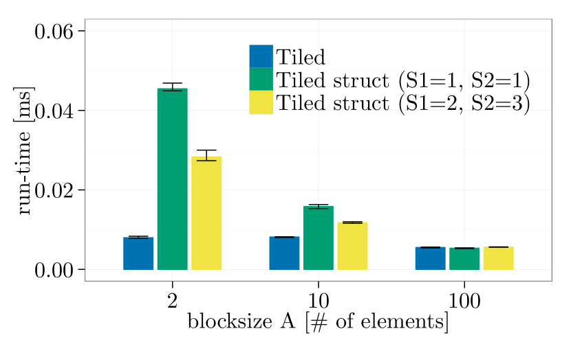
(b) $m=$2\text{\,}\mathrm{kB}$$, same node

(c) $m=$2.56\text{\,}\mathrm{MB}$$, $2$ nodes

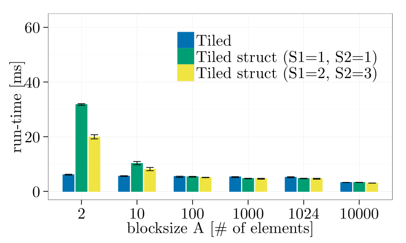
(d) $m=$2.56\text{\,}\mathrm{MB}$$, same node

Figure 64: Tiled ($AB$) vs. Tiled-struct, element datatype: MPI_INT, Ping-pong, MVAPICH2-2.1.

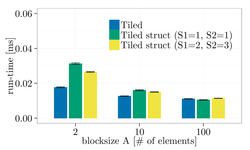
(a) $m=$2\text{\,}\mathrm{kB}$$, $2$ nodes

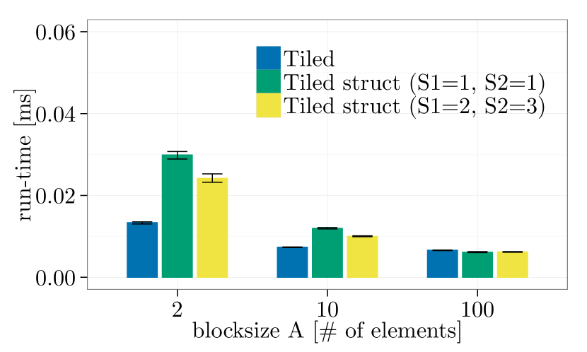
(b) $m=$2\text{\,}\mathrm{kB}$$, same node

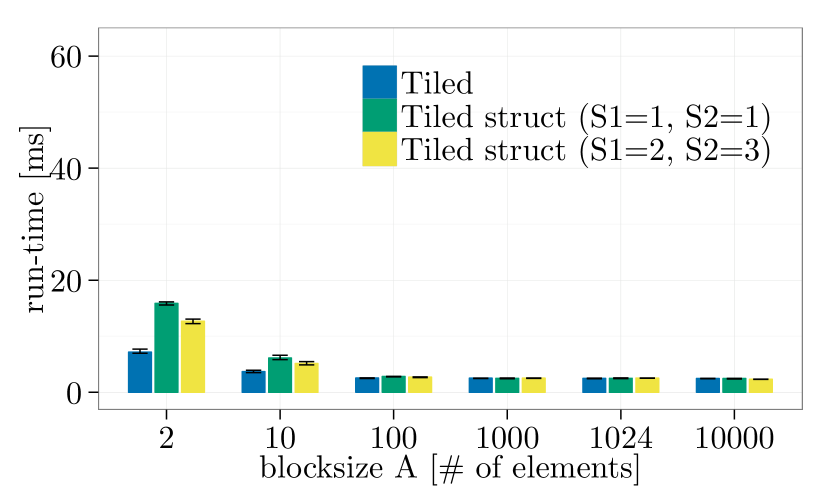
(c) $m=$2.56\text{\,}\mathrm{MB}$$, $2$ nodes

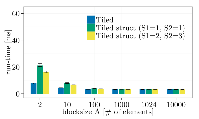
(d) $m=$2.56\text{\,}\mathrm{MB}$$, same node

Figure 65: Tiled ($AB$) vs. Tiled-struct, element datatype: MPI_INT, Ping-pong, OpenMPI-1.10.1.

A.6 Expectation Test 3.2.4 (Sect. 3.2.4)

 

• Tiled ($AB$), Tiled-vector

• Ping-pong

 

• Figure 66:   NEC MPI-1.3.1

• Figure 67:   MVAPICH2-2.1

• Figure 68:   OpenMPI-1.10.1

 

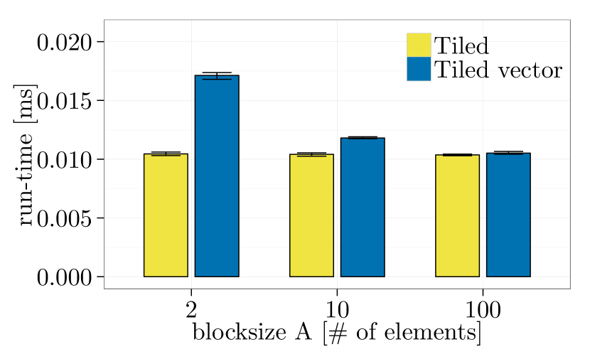
(a) $m=$2\text{\,}\mathrm{kB}$$, $2$ nodes

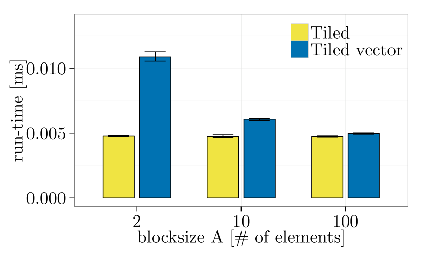
(b) $m=$2\text{\,}\mathrm{kB}$$, same node

(c) $m=$2.56\text{\,}\mathrm{MB}$$, $2$ nodes

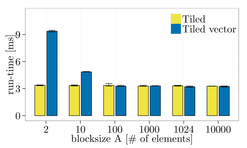
(d) $m=$2.56\text{\,}\mathrm{MB}$$, same node

Figure 66: Tiled ($AB$) vs. Tiled-vector, element datatype: MPI_INT, Ping-pong, NEC MPI-1.3.1.

(a) $m=$2\text{\,}\mathrm{kB}$$, $2$ nodes

(b) $m=$2\text{\,}\mathrm{kB}$$, same node

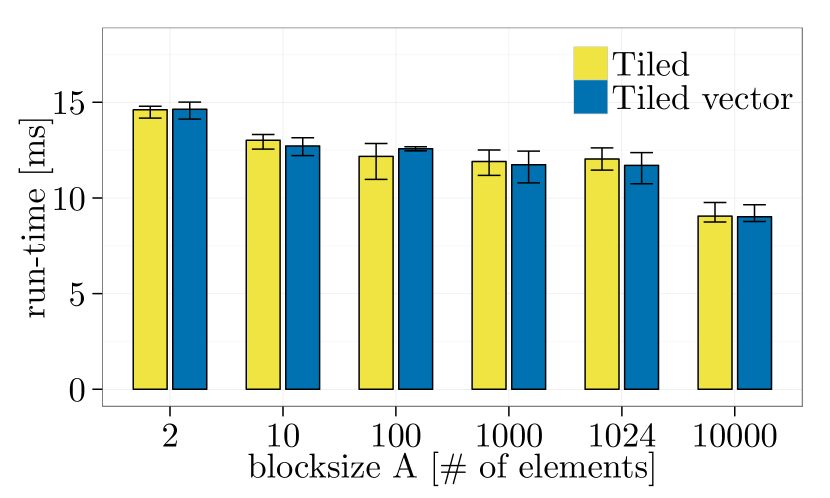
(c) $m=$2.56\text{\,}\mathrm{MB}$$, $2$ nodes

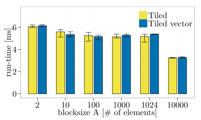
(d) $m=$2.56\text{\,}\mathrm{MB}$$, same node

Figure 67: Tiled ($AB$) vs. Tiled-vector, element datatype: MPI_INT, Ping-pong, MVAPICH2-2.1.

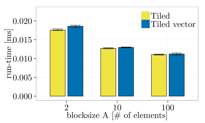
(a) $m=$2\text{\,}\mathrm{kB}$$, $2$ nodes

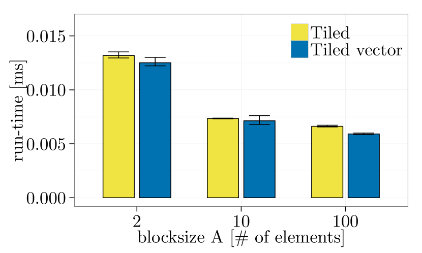
(b) $m=$2\text{\,}\mathrm{kB}$$, same node

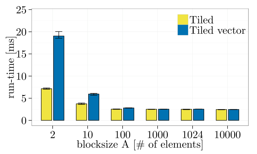
(c) $m=$2.56\text{\,}\mathrm{MB}$$, $2$ nodes

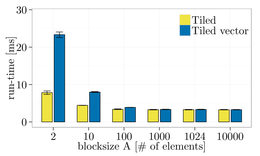
(d) $m=$2.56\text{\,}\mathrm{MB}$$, same node

Figure 68: Tiled ($AB$) vs. Tiled-vector, element datatype: MPI_INT, Ping-pong, OpenMPI-1.10.1.

A.7 Expectation Test 3.2.5 (Sect. 3.2.5)

 

• Tiled ($AB$), Vector-tiled

• Ping-pong

 

• Figure 69:   NEC MPI-1.3.1

• Figure 70:   MVAPICH2-2.1

• Figure 71:   OpenMPI-1.10.1

 

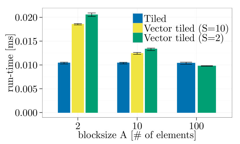
(a) $m=$2\text{\,}\mathrm{kB}$$, $2$ nodes

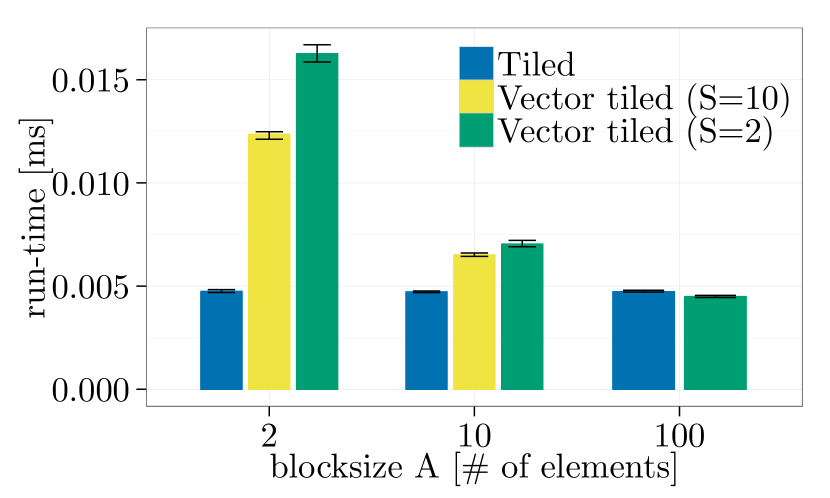
(b) $m=$2\text{\,}\mathrm{kB}$$, same node

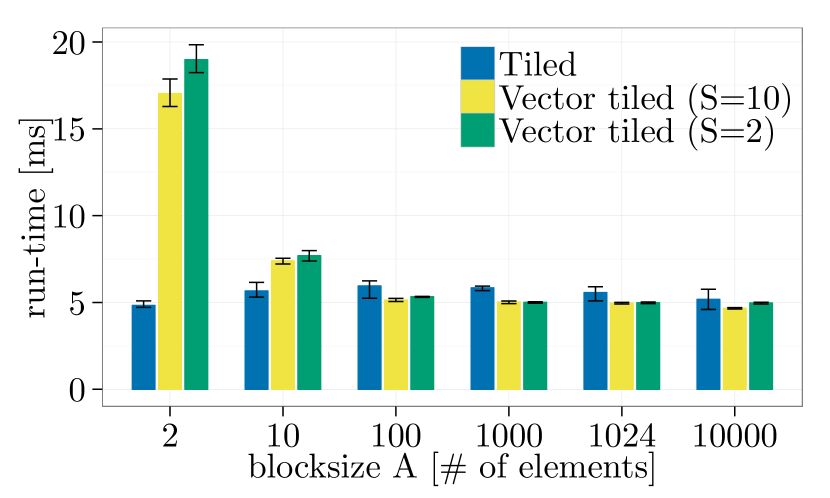
(c) $m=$2.56\text{\,}\mathrm{MB}$$, $2$ nodes

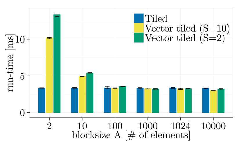
(d) $m=$2.56\text{\,}\mathrm{MB}$$, same node

Figure 69: Tiled ($AB$) vs. Vector-tiled, element datatype: MPI_INT, Ping-pong, NEC MPI-1.3.1.

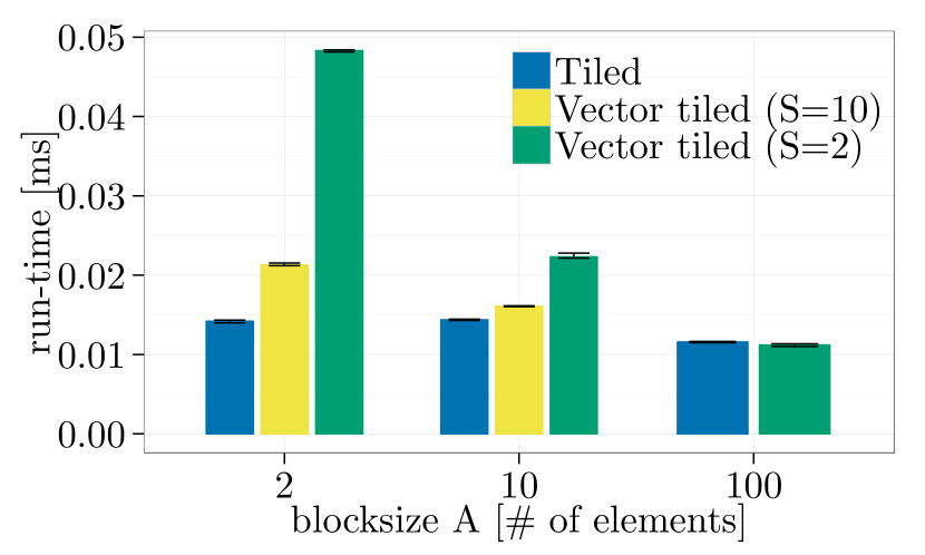
(a) $m=$2\text{\,}\mathrm{kB}$$, $2$ nodes

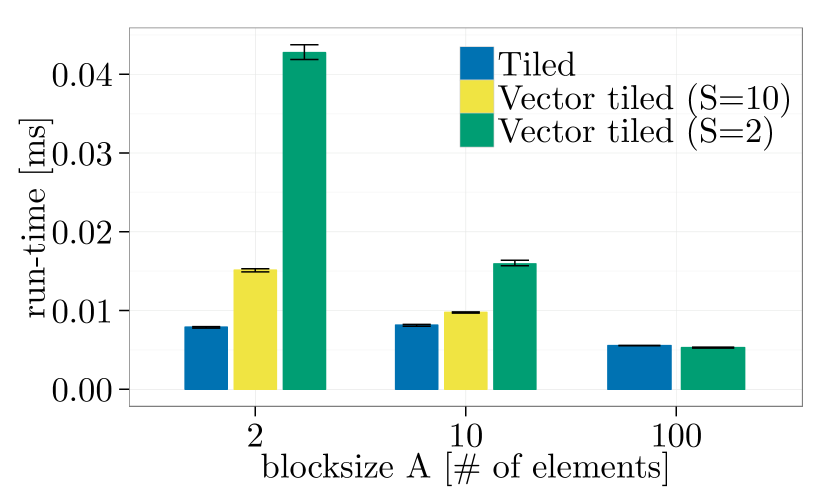
(b) $m=$2\text{\,}\mathrm{kB}$$, same node

(c) $m=$2.56\text{\,}\mathrm{MB}$$, $2$ nodes

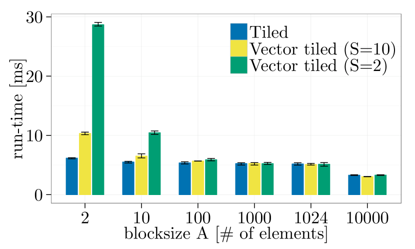
(d) $m=$2.56\text{\,}\mathrm{MB}$$, same node

Figure 70: Tiled ($AB$) vs. Vector-tiled, element datatype: MPI_INT, Ping-pong, MVAPICH2-2.1.

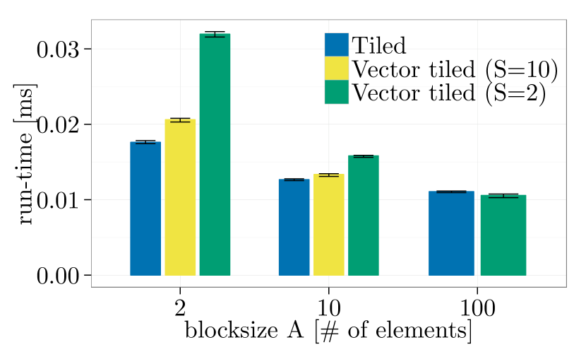
(a) $m=$2\text{\,}\mathrm{kB}$$, $2$ nodes

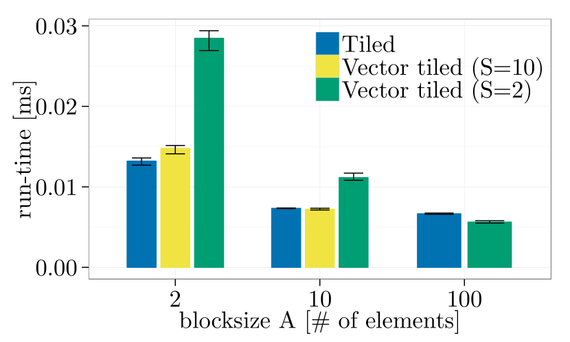
(b) $m=$2\text{\,}\mathrm{kB}$$, same node

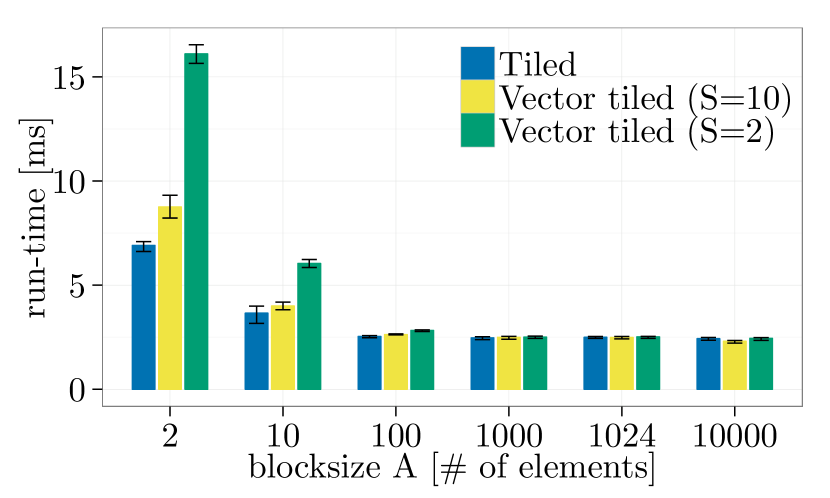
(c) $m=$2.56\text{\,}\mathrm{MB}$$, $2$ nodes

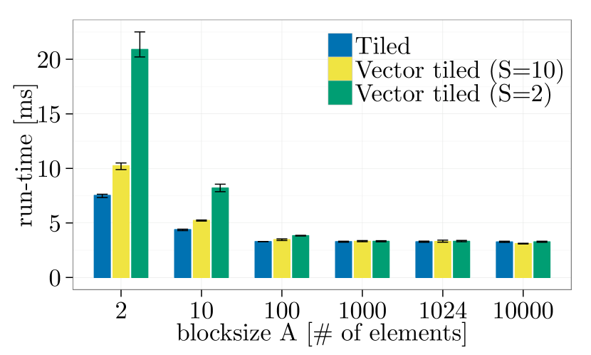
(d) $m=$2.56\text{\,}\mathrm{MB}$$, same node

Figure 71: Tiled ($AB$) vs. Vector-tiled, element datatype: MPI_INT, Ping-pong, OpenMPI-1.10.1.

A.8 Expectation Test 3.2.6 (Sect. 3.2.6)

 

• Block, Block-indexed

• Ping-pong

 

• Figure 72:   NEC MPI-1.3.1

• Figure 73:   MVAPICH2-2.1

• Figure 74:   OpenMPI-1.10.1

 

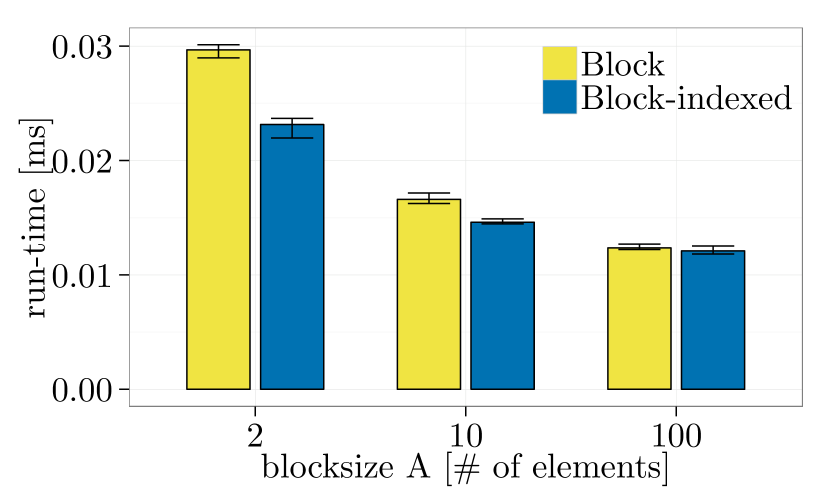
(a) $m=$3.2\text{\,}\mathrm{kB}$$, $2$ nodes

(b) $m=$3.2\text{\,}\mathrm{kB}$$, same node

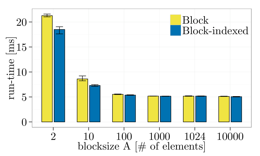
(c) $m=$2.56\text{\,}\mathrm{MB}$$, $2$ nodes

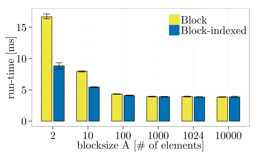
(d) $m=$2.56\text{\,}\mathrm{MB}$$, same node

Figure 72: Block vs. Block-indexed, element datatype: MPI_INT, Ping-pong, NEC MPI-1.3.1.

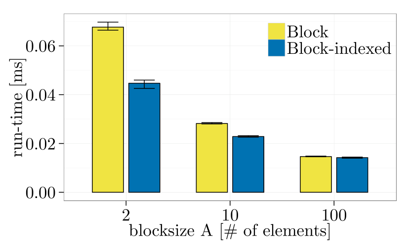
(a) $m=$3.2\text{\,}\mathrm{kB}$$, $2$ nodes

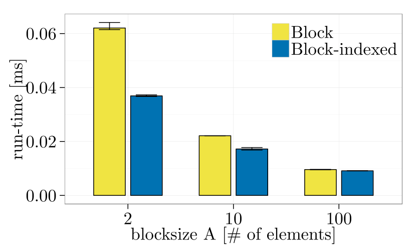
(b) $m=$3.2\text{\,}\mathrm{kB}$$, same node

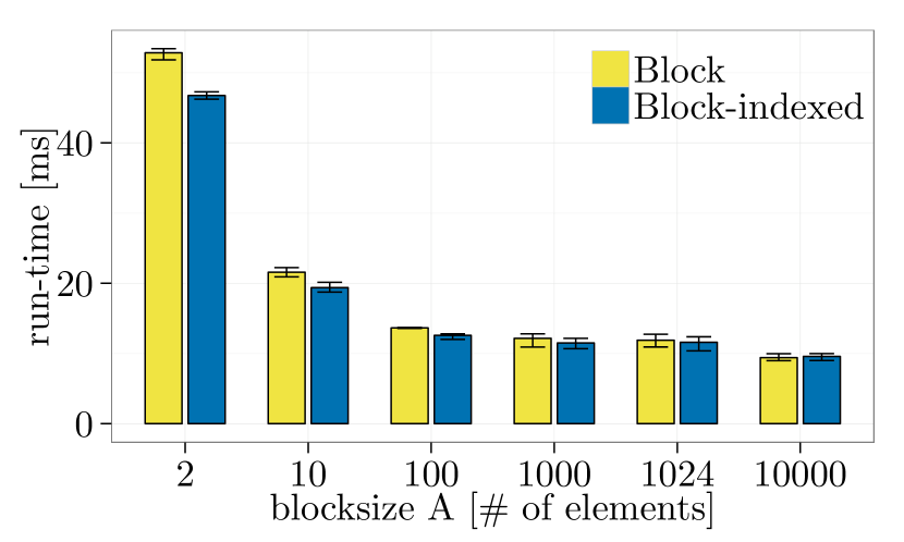
(c) $m=$2.56\text{\,}\mathrm{MB}$$, $2$ nodes

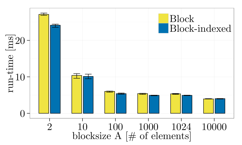
(d) $m=$2.56\text{\,}\mathrm{MB}$$, same node

Figure 73: Block vs. Block-indexed, element datatype: MPI_INT, Ping-pong, MVAPICH2-2.1.

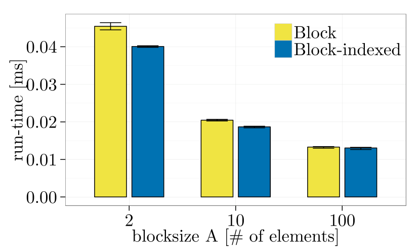
(a) $m=$3.2\text{\,}\mathrm{kB}$$, $2$ nodes

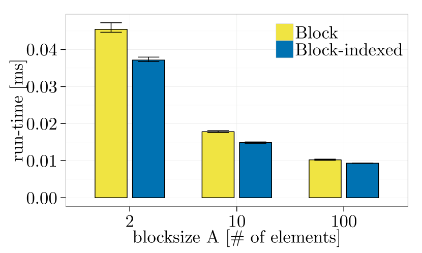
(b) $m=$3.2\text{\,}\mathrm{kB}$$, same node

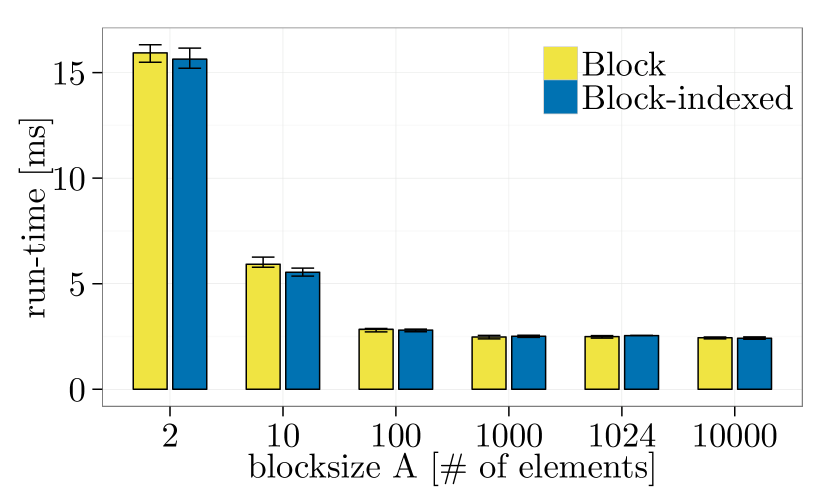
(c) $m=$2.56\text{\,}\mathrm{MB}$$, $2$ nodes

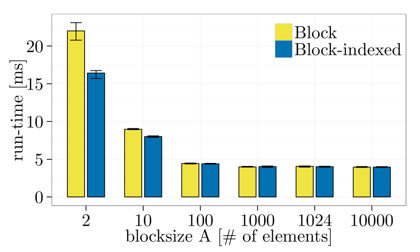
(d) $m=$2.56\text{\,}\mathrm{MB}$$, same node

Figure 74: Block vs. Block-indexed, element datatype: MPI_INT, Ping-pong, OpenMPI-1.10.1.

A.9 Expectation Test 3.2.7 (Sect. 3.2.7)

 

• Alternating, Alternating-indexed

• Ping-pong

 

• Figure 75:   NEC MPI-1.3.1

• Figure 76:   MVAPICH2-2.1

• Figure 77:   OpenMPI-1.10.1

 

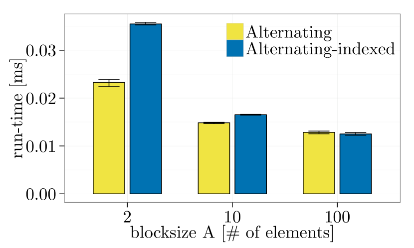
(a) $m=$3.2\text{\,}\mathrm{kB}$$, $2$ nodes

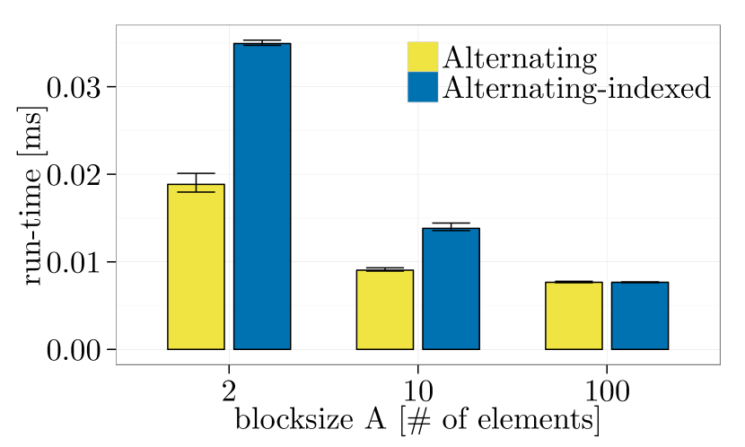
(b) $m=$3.2\text{\,}\mathrm{kB}$$, same node

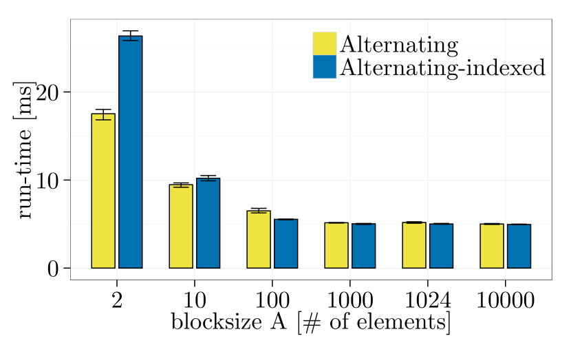
(c) $m=$2.56\text{\,}\mathrm{MB}$$, $2$ nodes

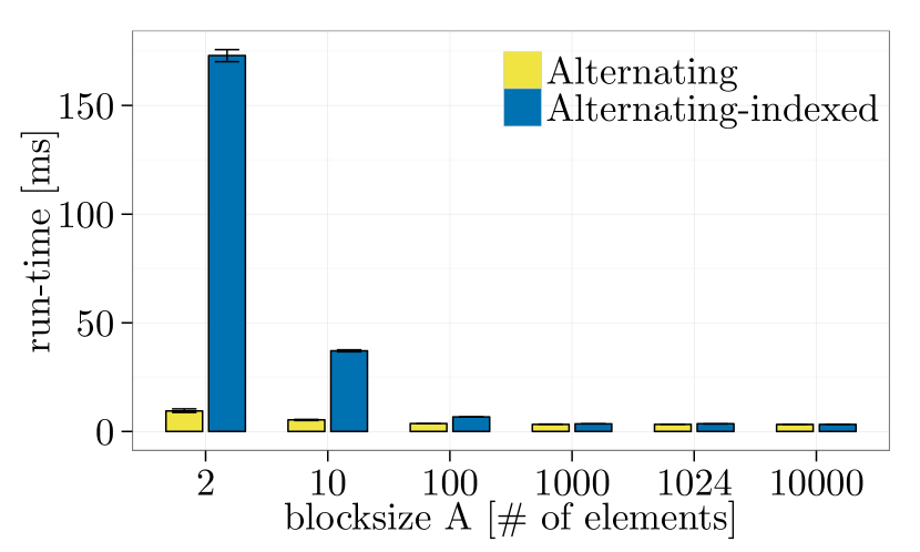
(d) $m=$2.56\text{\,}\mathrm{MB}$$, same node

Figure 75: Alternating vs. Alternating-indexed, element datatype: MPI_INT, Ping-pong, NEC MPI-1.3.1.

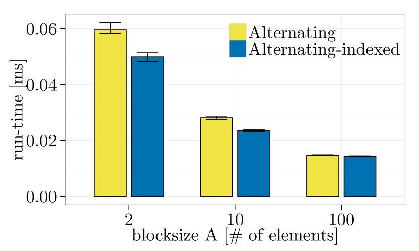
(a) $m=$3.2\text{\,}\mathrm{kB}$$, $2$ nodes

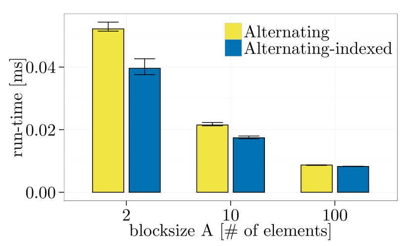
(b) $m=$3.2\text{\,}\mathrm{kB}$$, same node

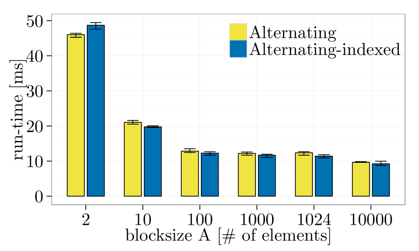
(c) $m=$2.56\text{\,}\mathrm{MB}$$, $2$ nodes

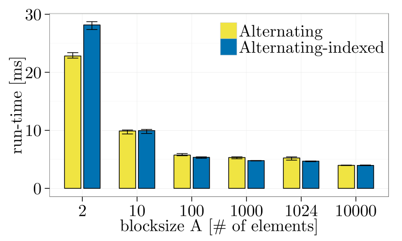
(d) $m=$2.56\text{\,}\mathrm{MB}$$, same node

Figure 76: Alternating vs. Alternating-indexed, element datatype: MPI_INT, Ping-pong, MVAPICH2-2.1.

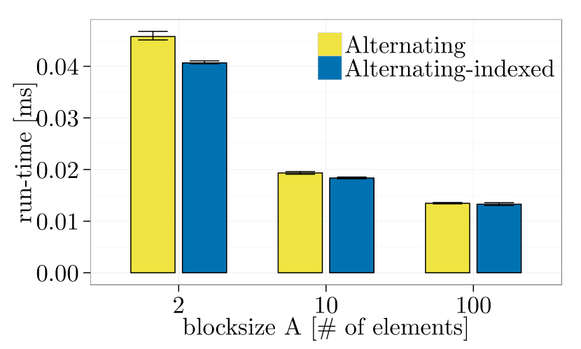
(a) $m=$3.2\text{\,}\mathrm{kB}$$, $2$ nodes

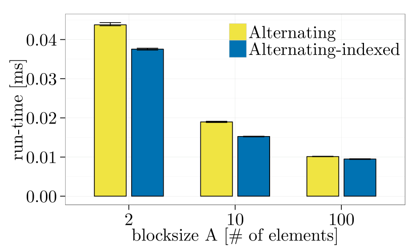
(b) $m=$3.2\text{\,}\mathrm{kB}$$, same node

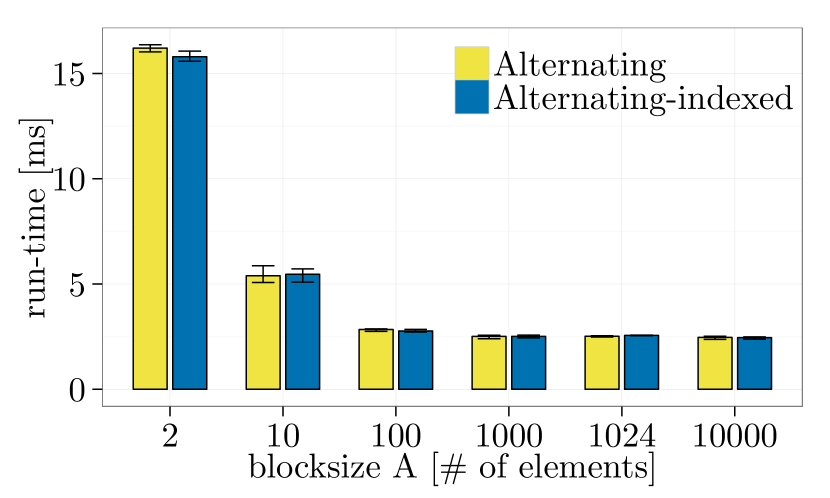
(c) $m=$2.56\text{\,}\mathrm{MB}$$, $2$ nodes

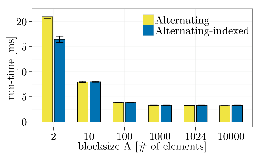
(d) $m=$2.56\text{\,}\mathrm{MB}$$, same node

Figure 77: Alternating vs. Alternating-indexed, element datatype: MPI_INT, Ping-pong, OpenMPI-1.10.1.

A.10 Expectation Test 3.2.8 (Sect. 3.2.8)

 

• Alternating-repeated, Alternating-struct

• Ping-pong

 

• Figure 78:   NEC MPI-1.3.1

• Figure 79:   MVAPICH2-2.1

• Figure 80:   OpenMPI-1.10.1

 

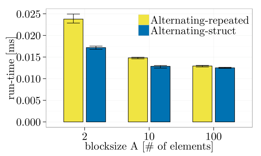
(a) $m=$3.2\text{\,}\mathrm{kB}$$, $2$ nodes

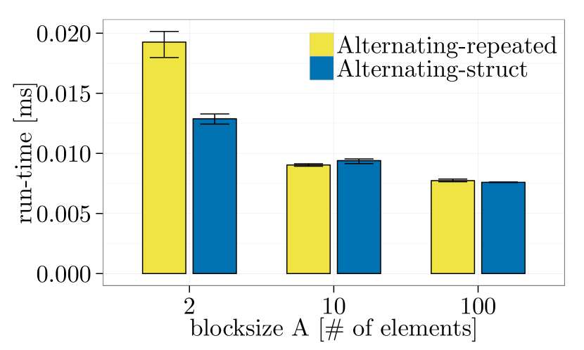
(b) $m=$3.2\text{\,}\mathrm{kB}$$, same node

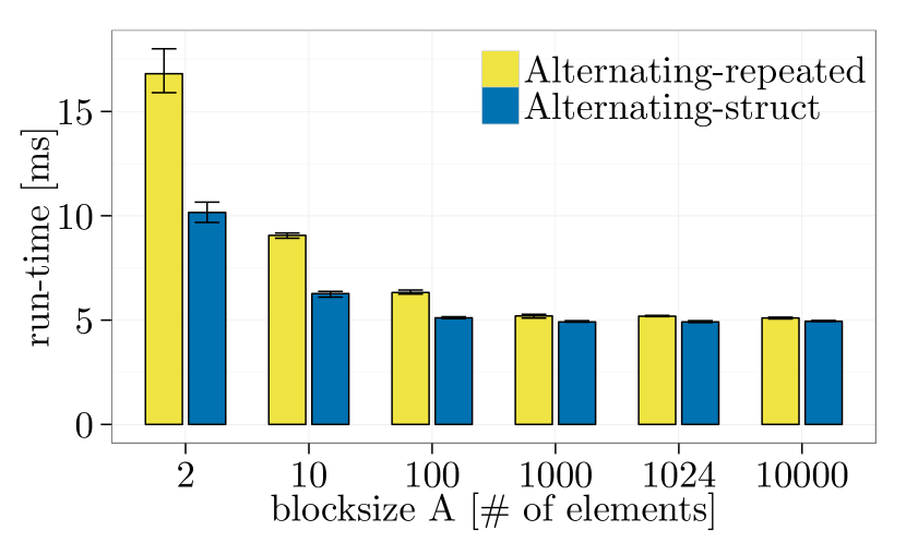
(c) $m=$2.56\text{\,}\mathrm{MB}$$, $2$ nodes

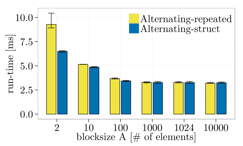
(d) $m=$2.56\text{\,}\mathrm{MB}$$, same node

Figure 78: Alternating-repeated vs. Alternating-struct, element datatype: MPI_INT, Ping-pong, NEC MPI-1.3.1.

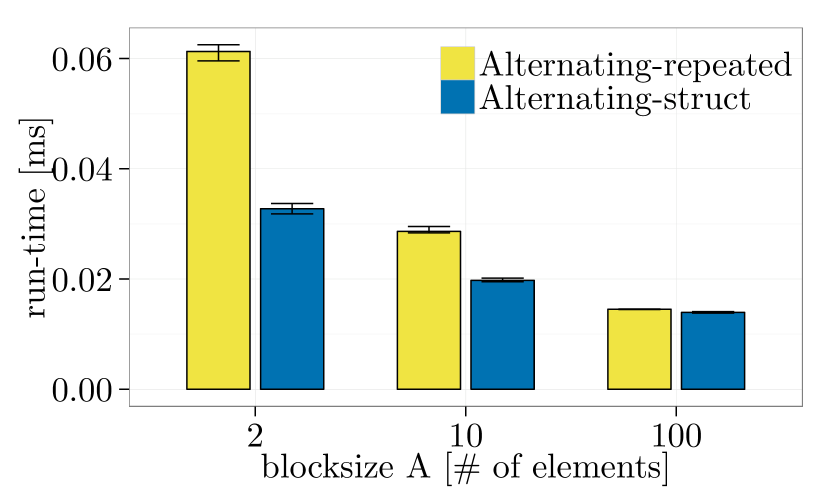
(a) $m=$3.2\text{\,}\mathrm{kB}$$, $2$ nodes

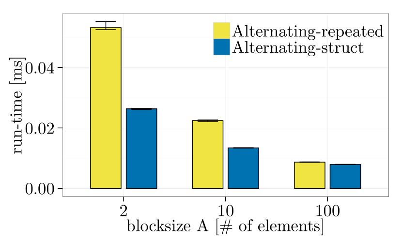
(b) $m=$3.2\text{\,}\mathrm{kB}$$, same node

(c) $m=$2.56\text{\,}\mathrm{MB}$$, $2$ nodes

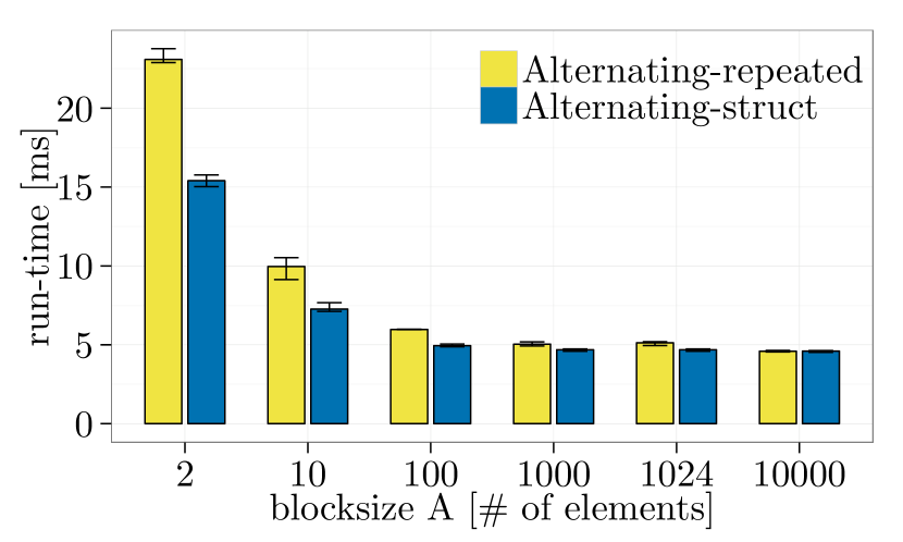
(d) $m=$2.56\text{\,}\mathrm{MB}$$, same node

Figure 79: Alternating-repeated vs. Alternating-struct, element datatype: MPI_INT, Ping-pong, MVAPICH2-2.1.

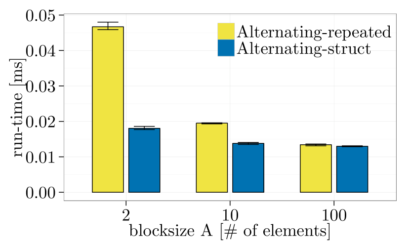
(a) $m=$3.2\text{\,}\mathrm{kB}$$, $2$ nodes

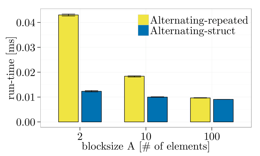
(b) $m=$3.2\text{\,}\mathrm{kB}$$, same node

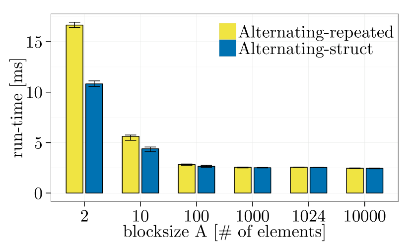
(c) $m=$2.56\text{\,}\mathrm{MB}$$, $2$ nodes

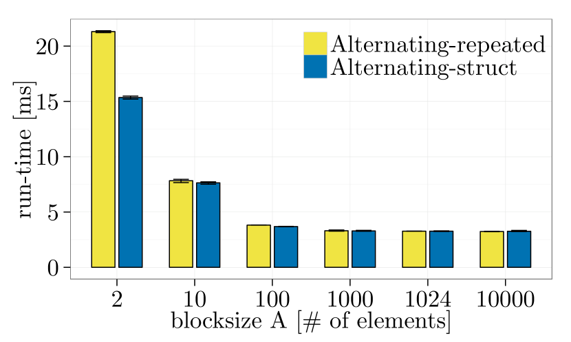
(d) $m=$2.56\text{\,}\mathrm{MB}$$, same node

Figure 80: Alternating-repeated vs. Alternating-struct, element datatype: MPI_INT, Ping-pong, OpenMPI-1.10.1.

A.11 Expectation Test 3.2.9 (Sect. 3.2.9)

 

• RowCol-fully-indexed, RowCol-contiguous-and-indexed, RowCol-struct

• Ping-pong

 

• Figure 81:   NEC MPI-1.3.1

• Figure 82:   MVAPICH2-2.1

• Figure 83:   OpenMPI-1.10.1

 

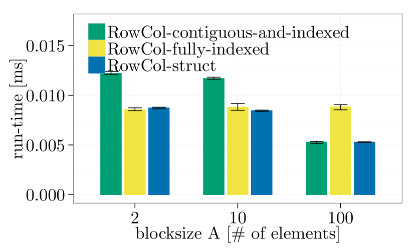
(a) $n=$100$$, $2$ nodes

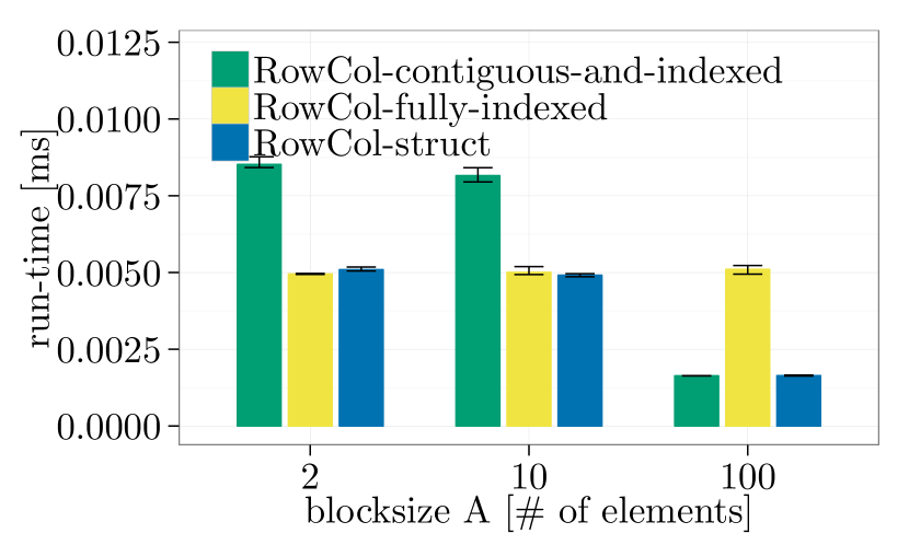
(b) $n=$100$$, same node

(c) $n=$10\,240$$, $2$ nodes

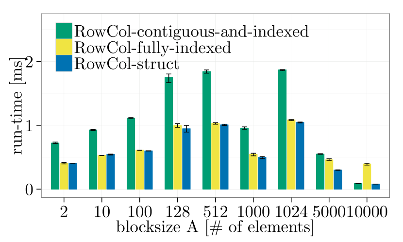
(d) $n=$10\,240$$, same node

Figure 81: RowCol-fully-indexed, RowCol-contiguous-and-indexed, RowCol-struct, element datatype: MPI_INT, buffer size (and extent) increases with blocksize $A$, Ping-pong, NEC MPI-1.3.1.

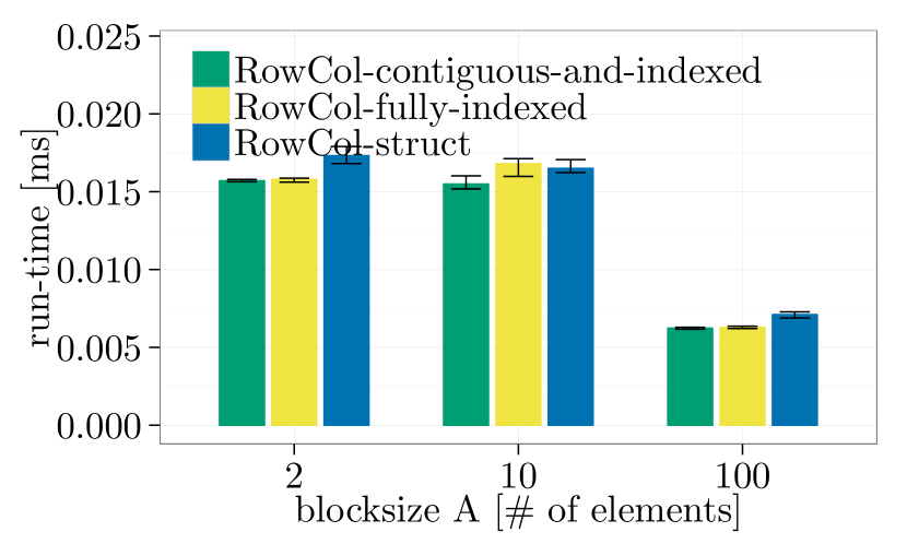
(a) $n=$100$$, $2$ nodes

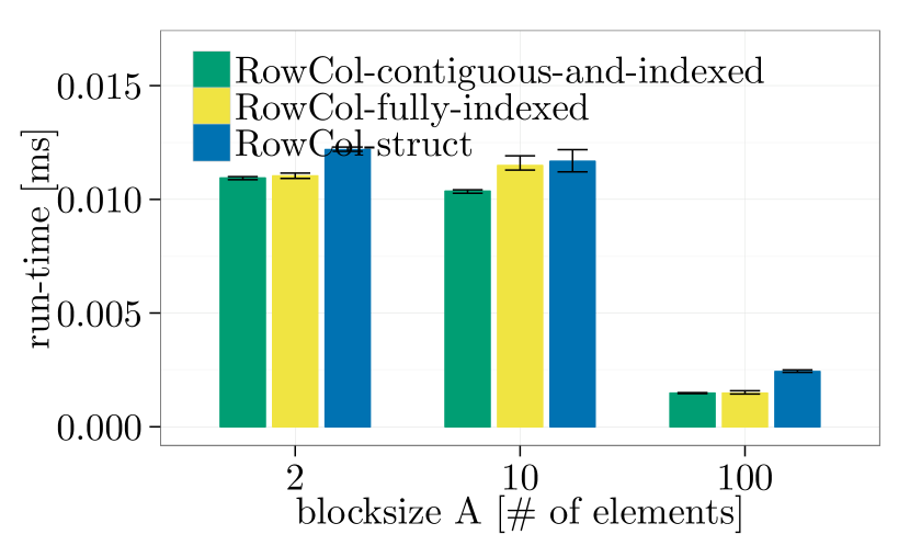
(b) $n=$100$$, same node

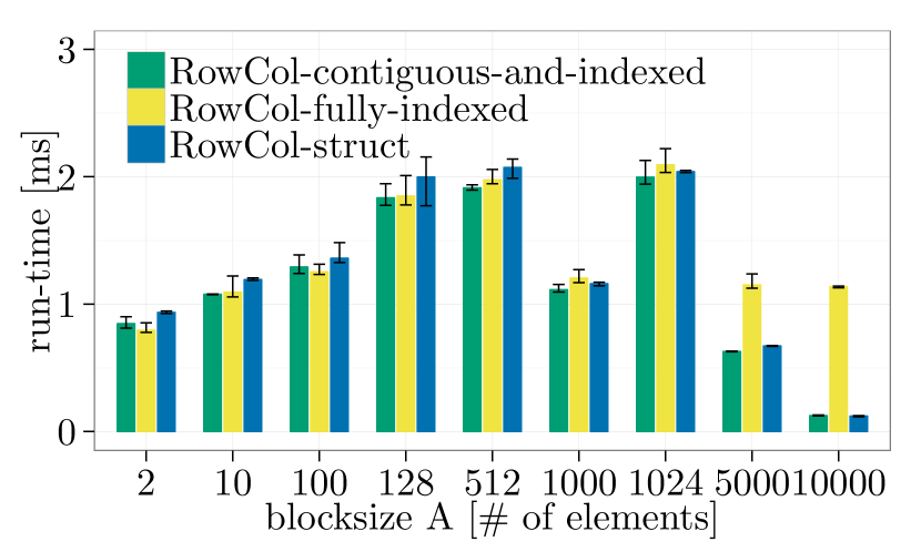
(c) $n=$10\,240$$, $2$ nodes

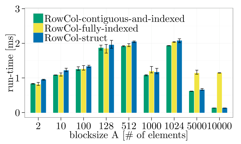
(d) $n=$10\,240$$, same node

Figure 82: RowCol-fully-indexed, RowCol-contiguous-and-indexed, RowCol-struct, element datatype: MPI_INT, buffer size (and extent) increases with blocksize $A$, Ping-pong, MVAPICH2-2.1.

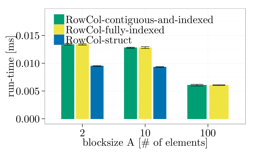
(a) $n=$100$$, $2$ nodes

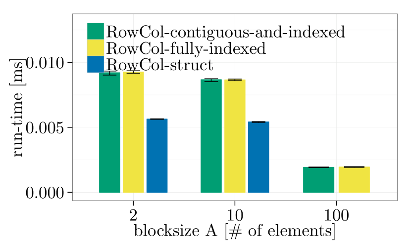
(b) $n=$100$$, same node

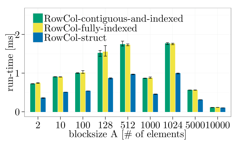
(c) $n=$10\,240$$, $2$ nodes

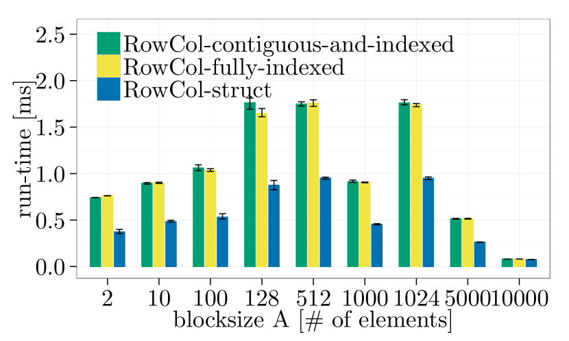
(d) $n=$10\,240$$, same node

Figure 83: RowCol-fully-indexed, RowCol-contiguous-and-indexed, RowCol-struct, element datatype: MPI_INT, buffer size (and extent) increases with blocksize $A$, Ping-pong, OpenMPI-1.10.1.

Appendix B Experimental Results on VSC-3

The experiments in this appendix have been performed using the hardware and software setup described below:

machine	$2000$ $\times$ Dual Intel Xeon E5-2650v2 @ $2.6\text{\,}\mathrm{GHz}$
	InfiniBand QDR-80
machine name	VSC-3
MPI libraries	Intel MPI-5.1.3
Compiler	Intel 16.0.1 (flags -O3)

B.1 Expectation Test 2.4.1 (Sect. 2.4.1)

 

• Contiguous, Tiled ($AB$), Block ($A\bar{B}$), Bucket ($\bar{A}B$), Alternating ($\bar{A}\bar{B}$)

• Ping-pong, MPI_Bcast, MPI_Allgather

 

• Figure 84:   Intel MPI-5.1.3, small datasize, Variant 1

• Figure 85:   Intel MPI-5.1.3, large datasize, Variant 1

• Figure 86:   Intel MPI-5.1.3, small datasize, Variant 1, one node

• Figure 87:   Intel MPI-5.1.3, large datasize, Variant 1, one node

• Figure 88:   Intel MPI-5.1.3, small datasize, Variant 2

• Figure 89:   Intel MPI-5.1.3, large datasize, Variant 2

• Figure 90:   Intel MPI-5.1.3, small datasize, Variant 2, one node

• Figure 91:   Intel MPI-5.1.3, large datasize, Variant 2, one node

 

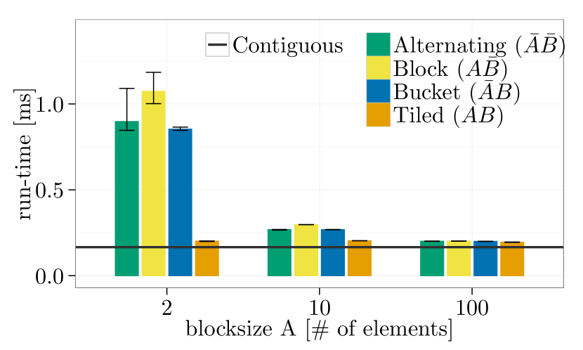
(a) MPI_Allgather

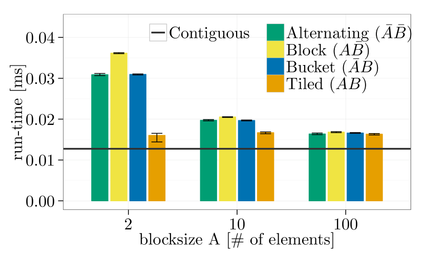
(b) MPI_Bcast

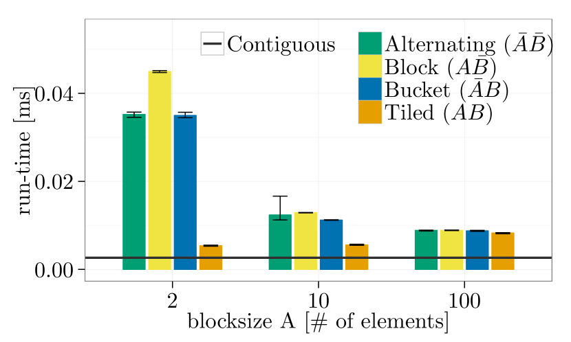
(c) Ping-pong

Figure 84: Contiguous vs. typed, $m=$3.2\text{\,}\mathrm{kB}$$, element datatype: MPI_INT, $32\text{\times}1$ processes ($2\text{\times}1$ for Ping-pong), Intel MPI-5.1.3, Variant 1.

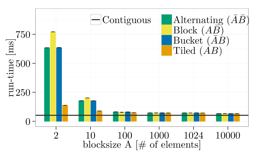
(a) MPI_Allgather

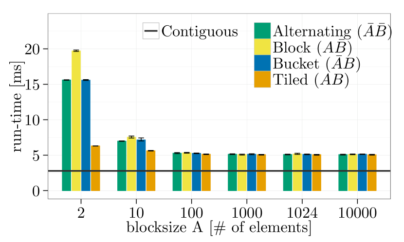
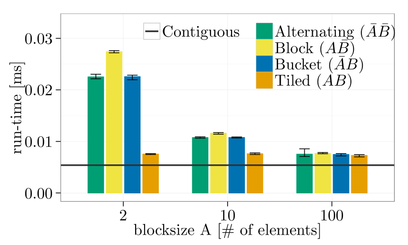
(b) MPI_Bcast

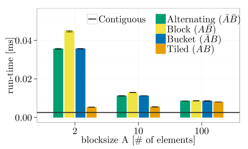
(c) Ping-pong

Figure 85: Contiguous vs. typed, $m=$2.56\text{\,}\mathrm{MB}$$, element datatype: MPI_INT, $32\text{\times}1$ processes ($2\text{\times}1$ for Ping-pong), Intel MPI-5.1.3, Variant 1.

(a) MPI_Allgather

(b) MPI_Bcast

(c) Ping-pong

Figure 86: Contiguous vs. typed, $m=$3.2\text{\,}\mathrm{kB}$$, element datatype: MPI_INT, one node, $16$ processes ($2$ for Ping-pong), Intel MPI-5.1.3, Variant 1.

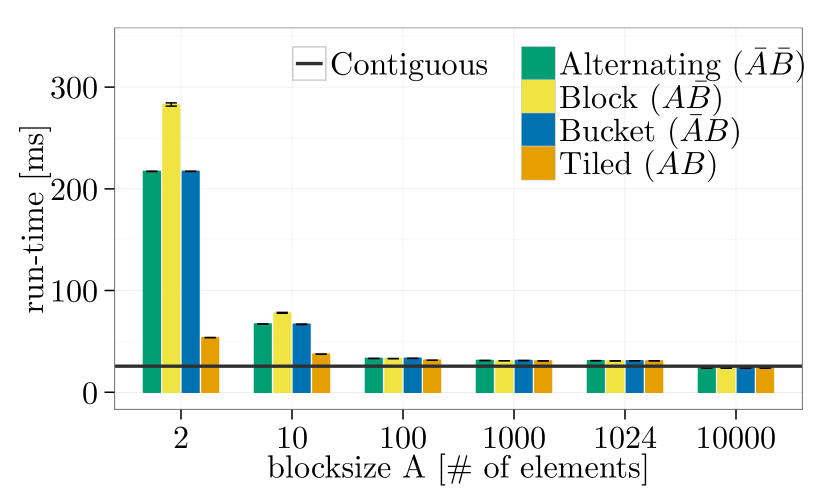
(a) MPI_Allgather

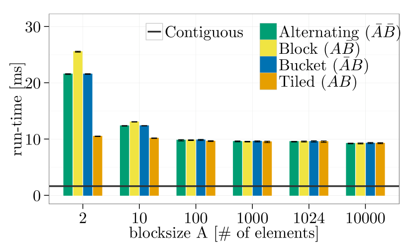
(b) MPI_Bcast

(c) Ping-pong

Figure 87: Contiguous vs. typed, $m=$2.56\text{\,}\mathrm{MB}$$, element datatype: MPI_INT, one node, $16$ processes ($2$ processes for Ping-pong), Intel MPI-5.1.3, Variant 1.

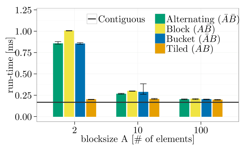
(a) MPI_Allgather

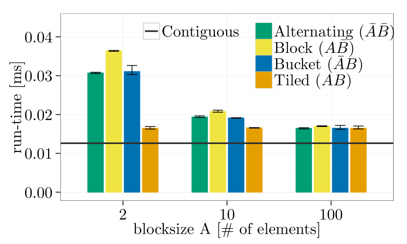
(b) MPI_Bcast

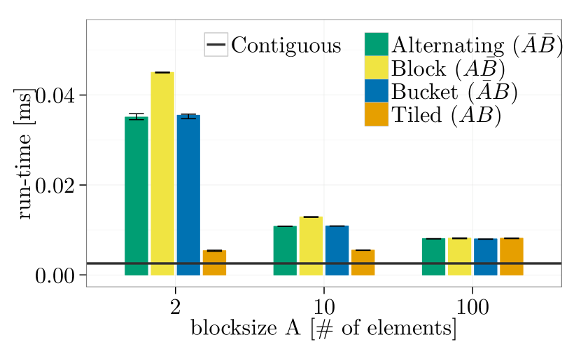
(c) Ping-pong

Figure 88: Contiguous vs. typed, $m=$3.2\text{\,}\mathrm{kB}$$, element datatype: MPI_INT, $32\text{\times}1$ processes ($2\text{\times}1$ for Ping-pong), Intel MPI-5.1.3, Variant 2.

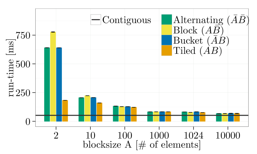
(a) MPI_Allgather

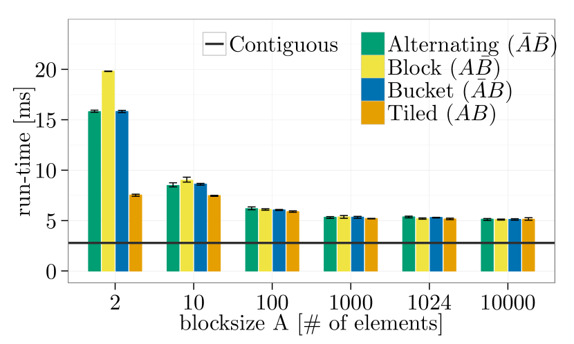
(b) MPI_Bcast

(c) Ping-pong

Figure 89: Contiguous vs. typed, $m=$2.56\text{\,}\mathrm{MB}$$, element datatype: MPI_INT, $32\text{\times}1$ processes ($2\text{\times}1$ for Ping-pong), Intel MPI-5.1.3, Variant 2.

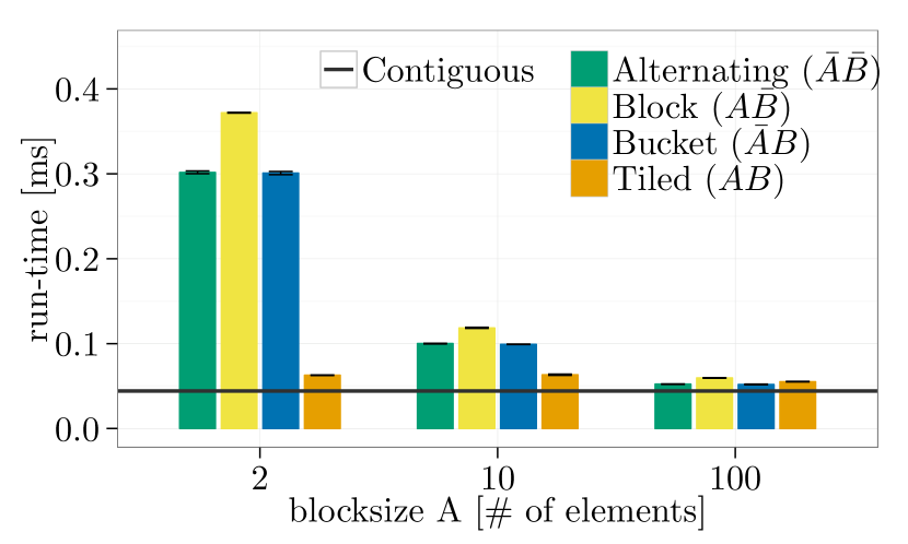
(a) MPI_Allgather

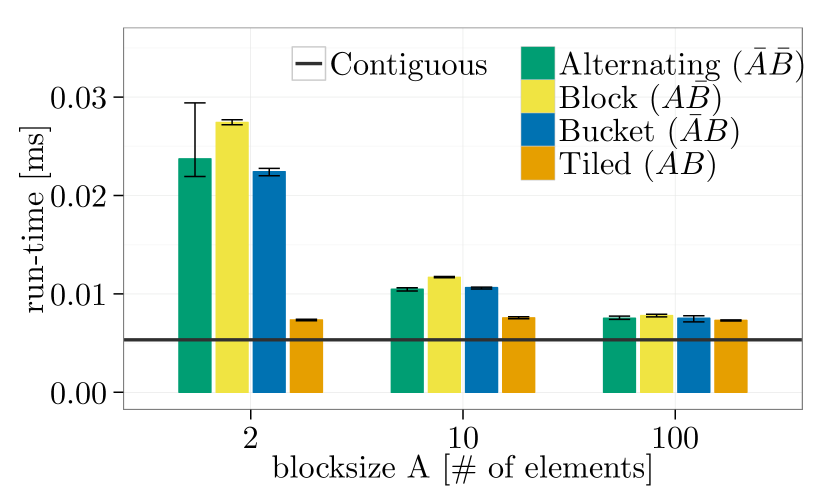
(b) MPI_Bcast

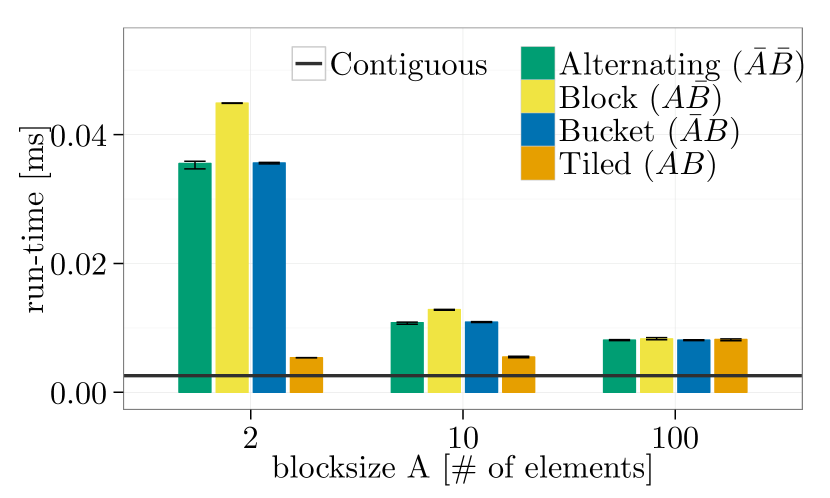
(c) Ping-pong

Figure 90: Contiguous vs. typed, $m=$3.2\text{\,}\mathrm{kB}$$, element datatype: MPI_INT, one node, $16$ processes ($2$ for Ping-pong), Intel MPI-5.1.3, Variant 2.

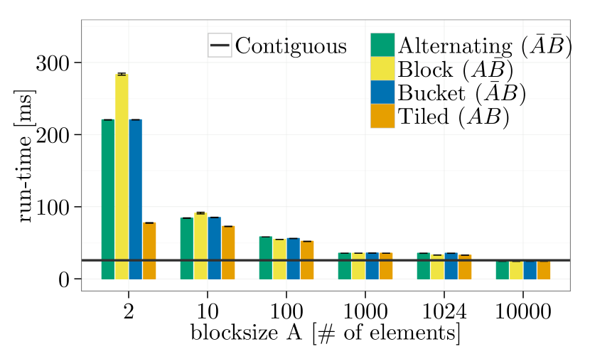
(a) MPI_Allgather

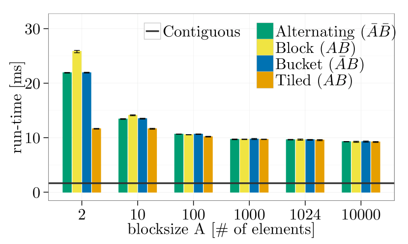
(b) MPI_Bcast

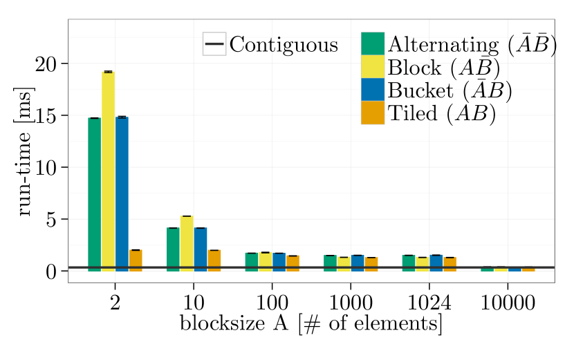
(c) Ping-pong

Figure 91: Contiguous vs. typed, $m=$2.56\text{\,}\mathrm{MB}$$, element datatype: MPI_INT, one node, $16$ processes ($2$ for Ping-pong), Intel MPI-5.1.3, Variant 2.

B.2 Expectation Test 2.4.2 (Sect. 2.4.2)

 

• Contiguous, Tiled-heterogeneous ($AB\bar{T}$)

• Ping-pong

 

• Figure 92:   Intel MPI-5.1.3

 

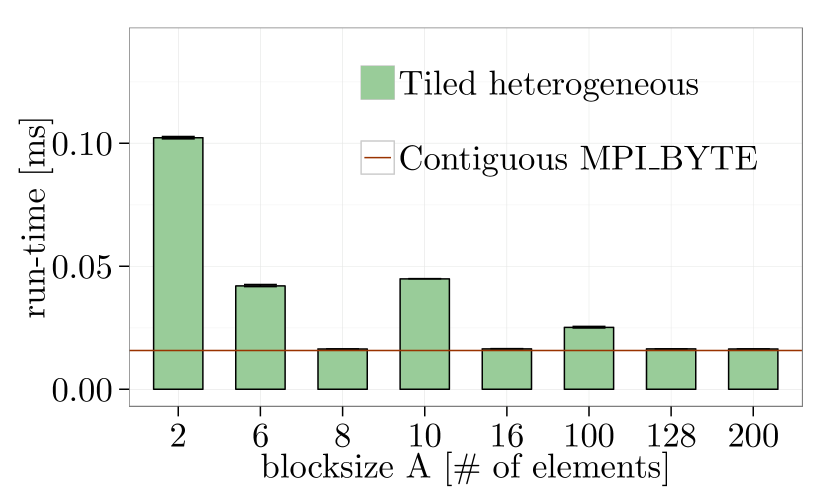
(a) $m=$48\text{\,}\mathrm{kB}$$, $2$ nodes

(b) $m=$48\text{\,}\mathrm{kB}$$, same node

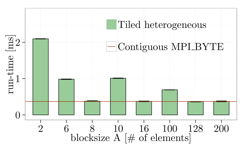
(c) $m=$1.5\text{\,}\mathrm{MB}$$, $2$ nodes

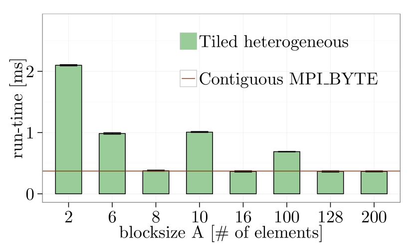
(d) $m=$1.5\text{\,}\mathrm{MB}$$, same node

Figure 92: Contiguous vs. Tiled-heterogeneous ($AB\bar{T}$) $A$=$B$, element datatype: MPI_INT, Ping-pong, Intel MPI-5.1.3.

B.3 Expectation Test 3.2.1 (Sect. 3.2.1)

 

• pack vs. unpack for basic layouts (Tiled, Block, Bucket, Alternating)

• MPI_Allgather, MPI_Bcast, Ping-pong

 

• Figure 93:   Intel MPI-5.1.3, Ping-pong, $2\text{\times}1$ processes

• Figure 94:   Intel MPI-5.1.3, Ping-pong, one node, $2$ processes

 

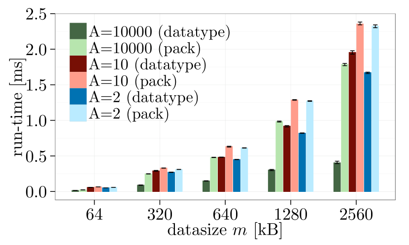
(a) Tiled

(b) Block

(c) Bucket

(d) Alternating

Figure 93: Basic layouts vs. pack/unpack, element datatype: MPI_INT, $2\text{\times}1$ processes, Ping-pong, Intel MPI-5.1.3.

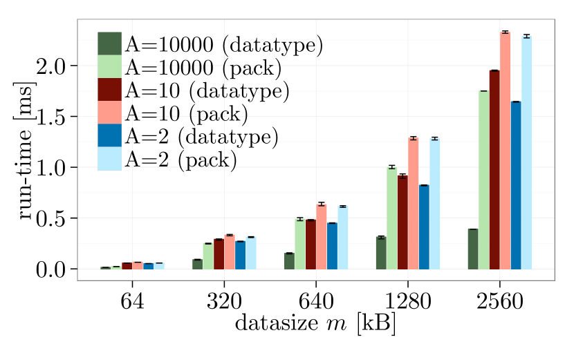
(a) Tiled

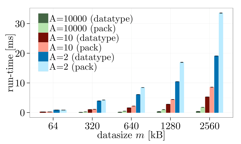
(b) Block

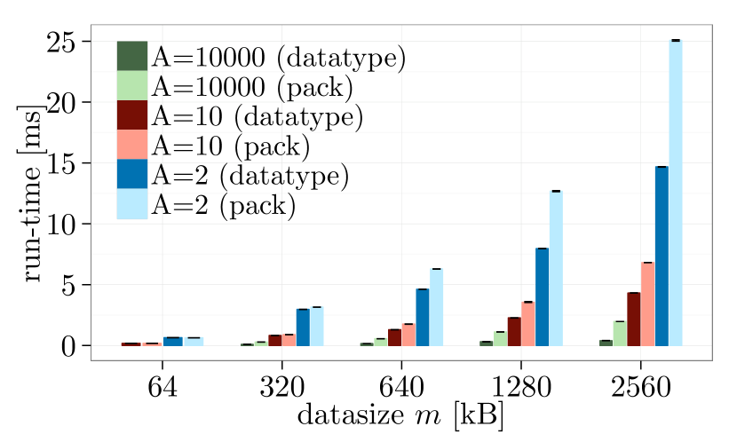
(c) Bucket

(d) Alternating

Figure 94: Basic layouts vs. pack/unpack, element datatype: MPI_INT, one node, $2$ processes, Ping-pong, Intel MPI-5.1.3.

B.4 Expectation Test 3.2.2 (Sect. 3.2.2)

 

• Contiguous-subtype vs. basic layouts (Tiled, Block, Bucket, Alternating)

• Ping-pong, MPI_Allgather, MPI_Bcast

 

• Figure 95:   Intel MPI-5.1.3, Ping-pong, small datasize

• Figure 96:   Intel MPI-5.1.3, Ping-pong, large datasize

• Figure 97:   Intel MPI-5.1.3, MPI_Allgather, small datasize

• Figure 98:   Intel MPI-5.1.3, MPI_Allgather, large datasize

• Figure 99:   Intel MPI-5.1.3, MPI_Bcast, small datasize

• Figure 100:   Intel MPI-5.1.3, MPI_Bcast, large datasize

 

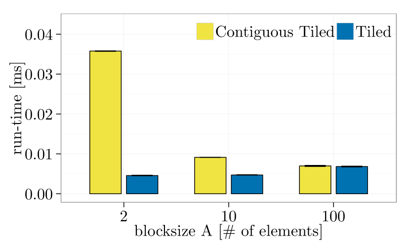
(a) Tiled

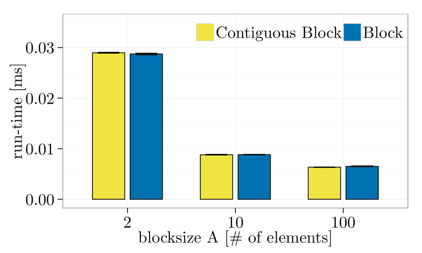
(b) Block

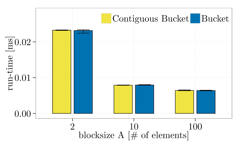
(c) Bucket

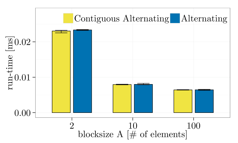
(d) Alternating

Figure 95: Basic layouts vs. Contiguous-subtype, $m=$2\text{\,}\mathrm{kB}$$, element datatype: MPI_INT, $2\text{\times}1$ processes, Ping-pong, Intel MPI-5.1.3 (similar results for $1\text{\times}2$ processes).

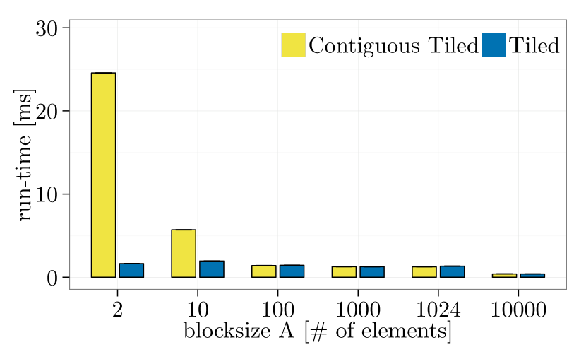
(a) Tiled

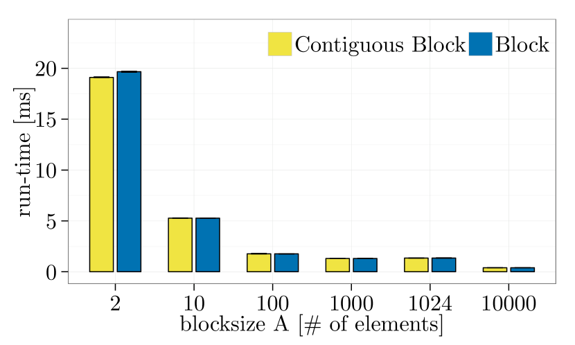
(b) Block

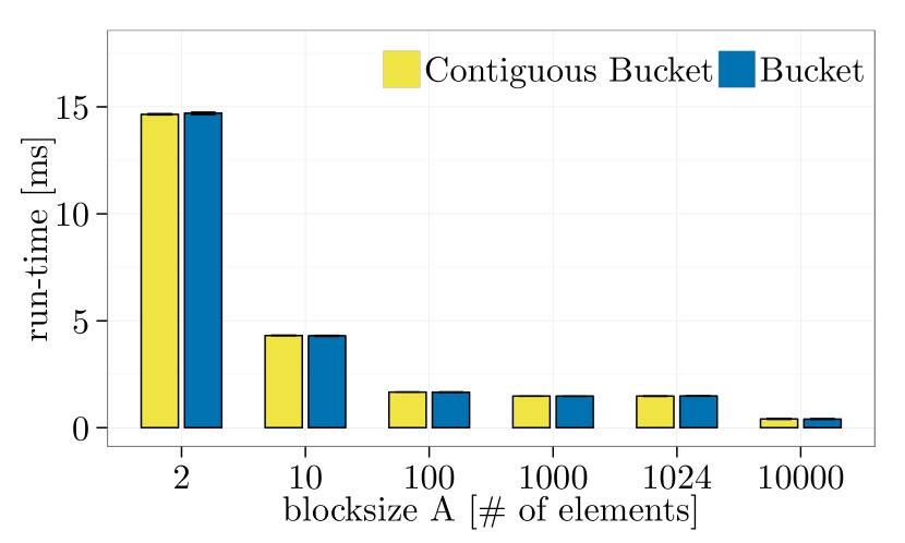
(c) Bucket

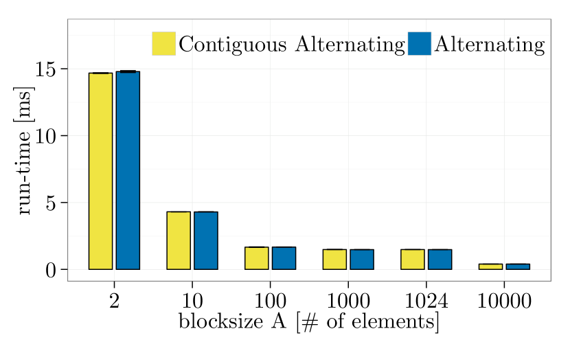
(d) Alternating

Figure 96: Basic layouts vs. Contiguous-subtype, $m=$2.56\text{\,}\mathrm{MB}$$, element datatype: MPI_INT, $2\text{\times}1$ processes, Ping-pong, Intel MPI-5.1.3 (similar results for $1\text{\times}2$ processes).

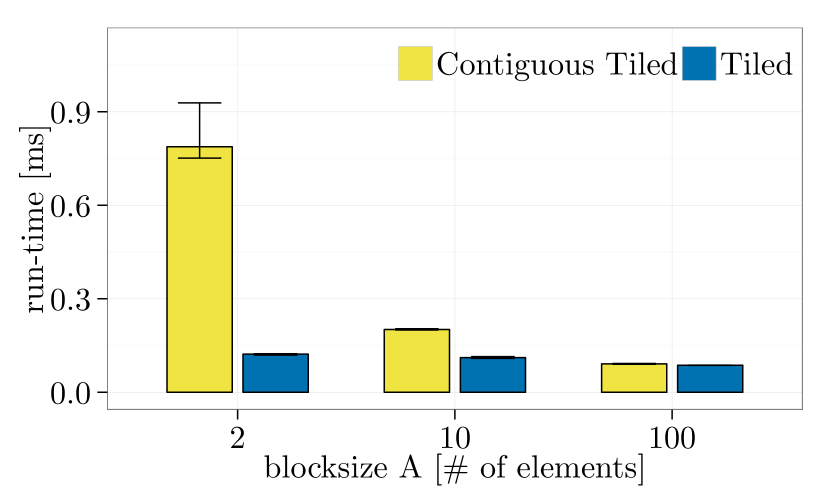
(a) Tiled

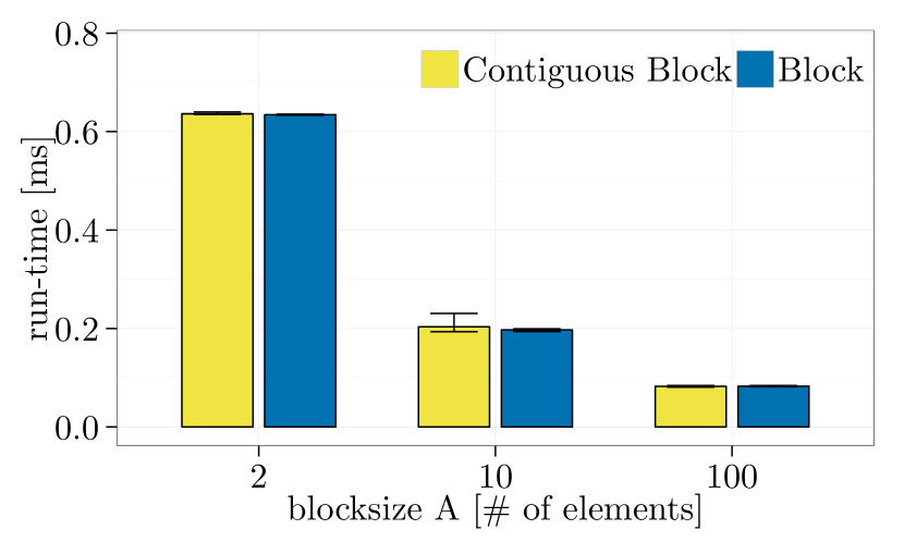
(b) Block

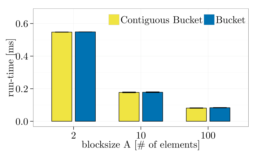
(c) Bucket

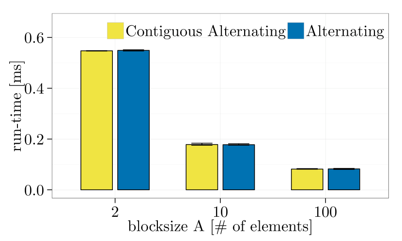
(d) Alternating

Figure 97: Basic layouts vs. Contiguous-subtype, $m=$2\text{\,}\mathrm{kB}$$, element datatype: MPI_INT, $32\text{\times}1$ processes, MPI_Allgather, Intel MPI-5.1.3 (similar results for $1\text{\times}16$ processes).

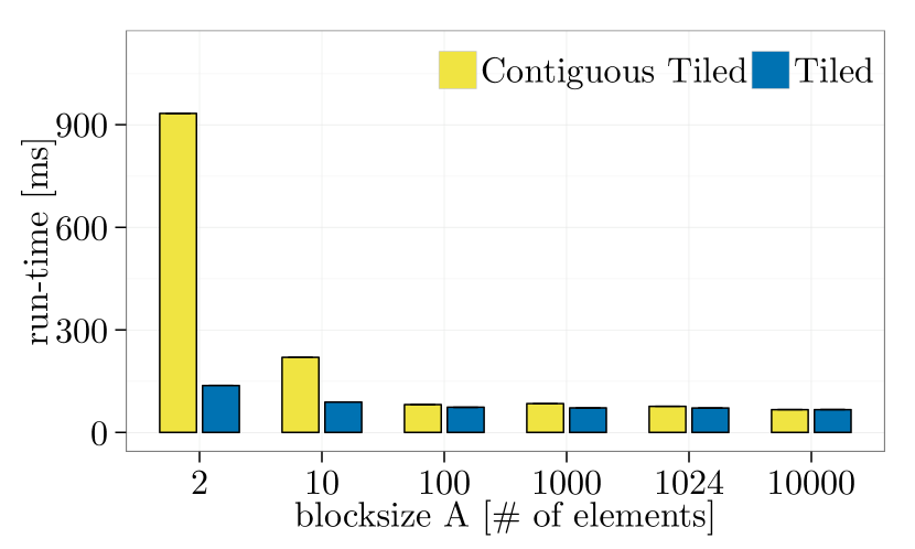
(a) Tiled

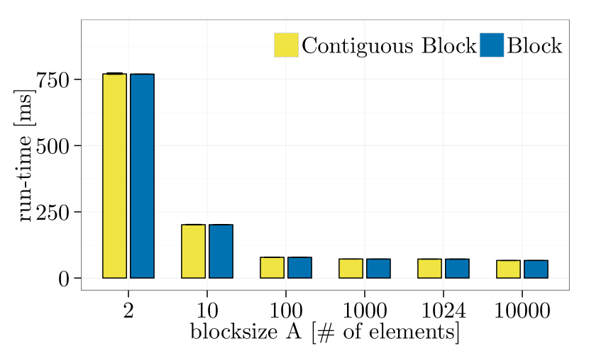
(b) Block

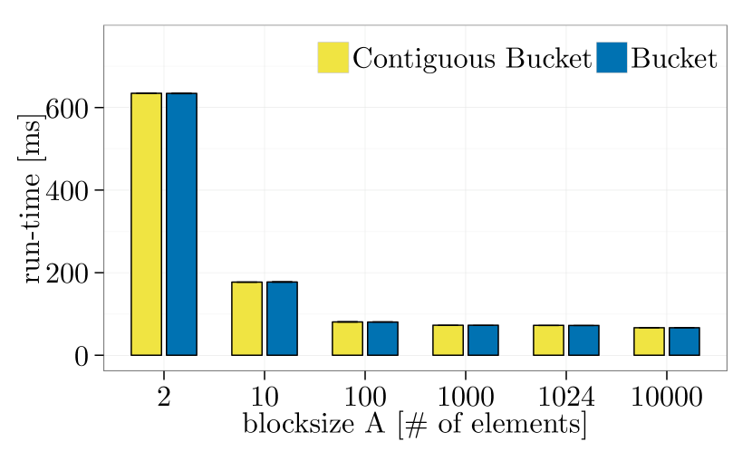
(c) Bucket

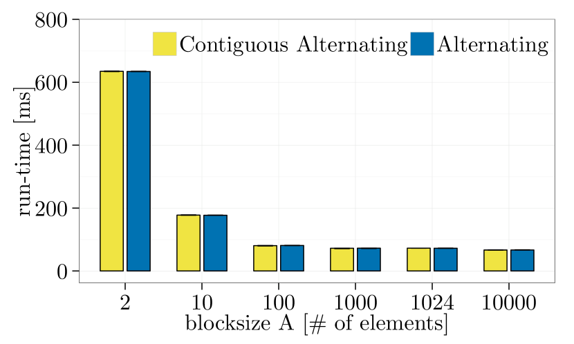
(d) Alternating

Figure 98: Basic layouts vs. Contiguous-subtype, $m=$2.56\text{\,}\mathrm{MB}$$, element datatype: MPI_INT, $32\text{\times}1$ processes, MPI_Allgather, Intel MPI-5.1.3 (similar results for $1\text{\times}16$ processes).

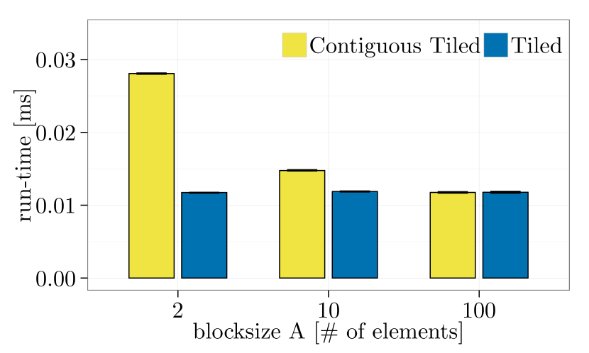
(a) Tiled

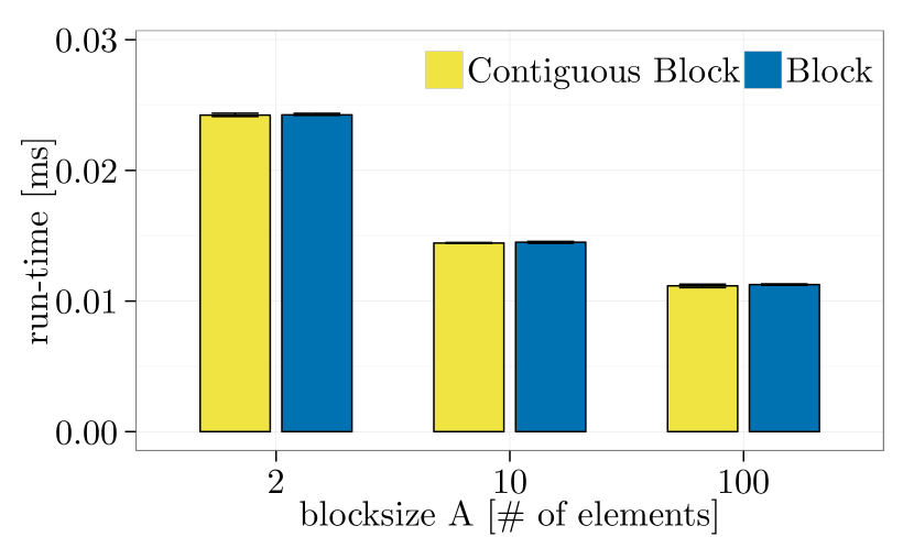
(b) Block

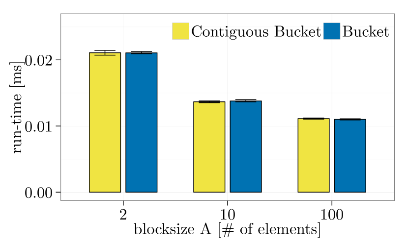
(c) Bucket

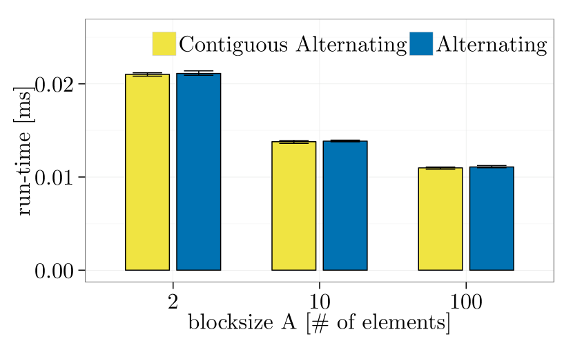
(d) Alternating

Figure 99: Basic layouts vs. Contiguous-subtype, $m=$2\text{\,}\mathrm{kB}$$, element datatype: MPI_INT, $32\text{\times}1$ processes, MPI_Bcast, Intel MPI-5.1.3 (similar results for $1\text{\times}16$ processes).

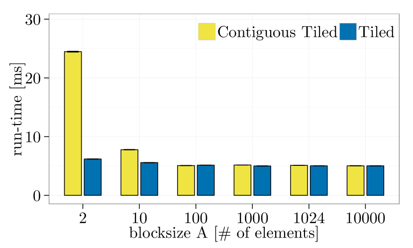
(a) Tiled

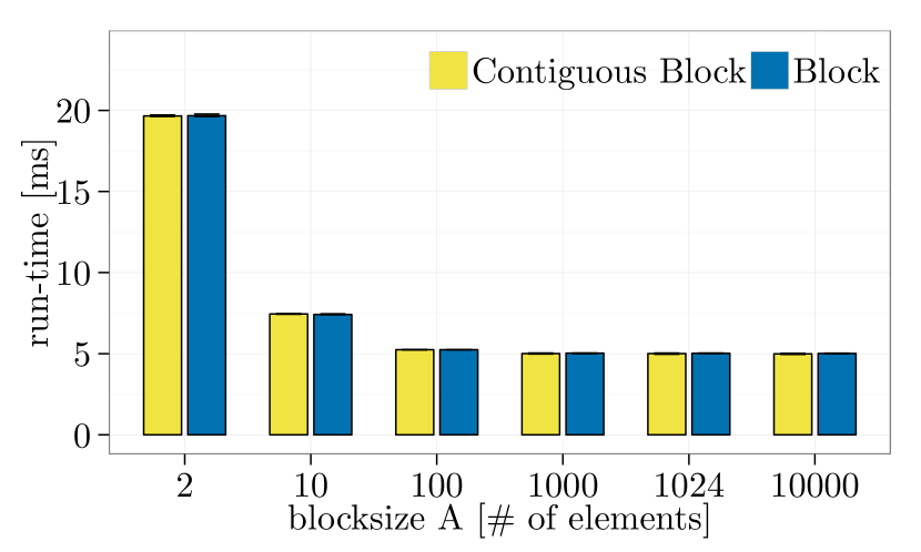
(b) Block

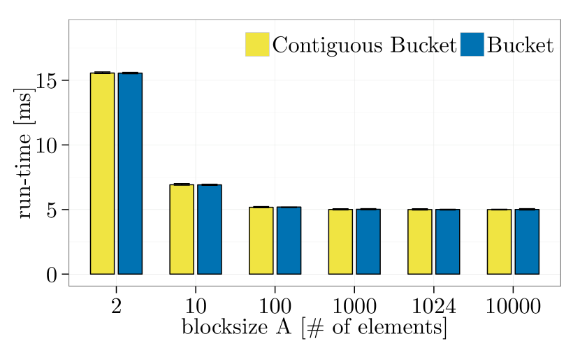
(c) Bucket

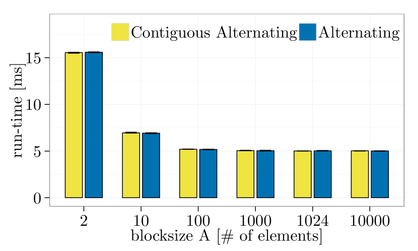
(d) Alternating

Figure 100: Basic layouts vs. Contiguous-subtype, $m=$2.56\text{\,}\mathrm{MB}$$, element datatype: MPI_INT, $32\text{\times}1$ processes, MPI_Bcast, Intel MPI-5.1.3 (similar results for $1\text{\times}16$ processes).

B.5 Expectation Test 3.2.5 (Sect. 3.2.5)

 

• Tiled ($AB$), Vector-tiled

• Ping-pong

 

• Figure 101:   Intel MPI-5.1.3

 

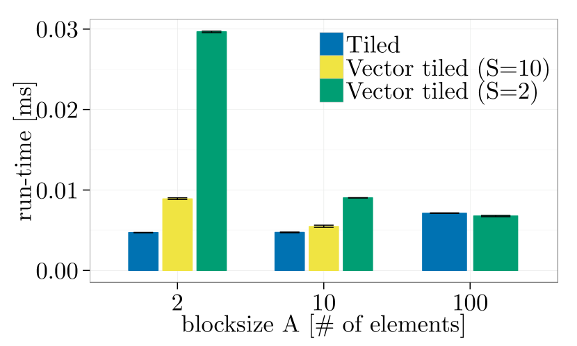
(a) $m=$2\text{\,}\mathrm{kB}$$, $2$ nodes

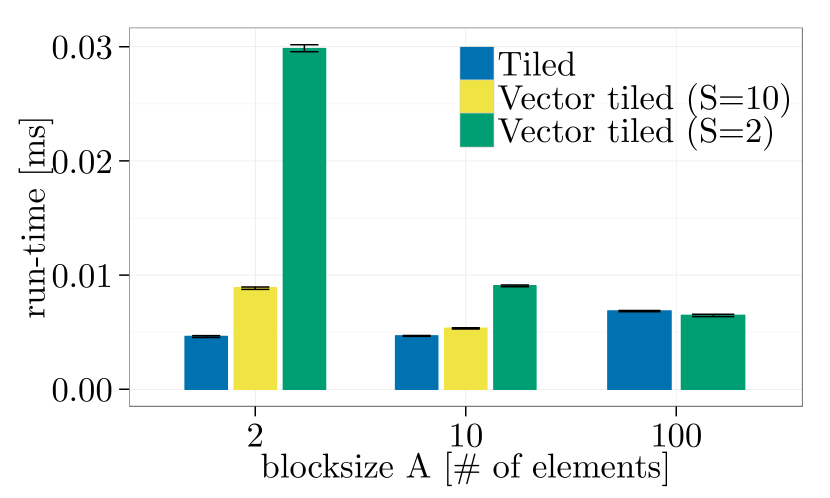
(b) $m=$2\text{\,}\mathrm{kB}$$, same node

(c) $m=$2.56\text{\,}\mathrm{MB}$$, $2$ nodes

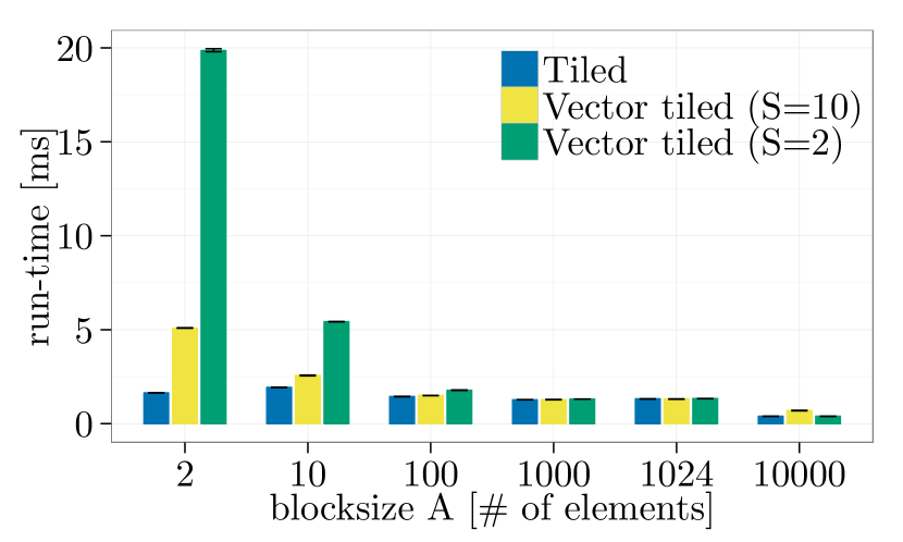
(d) $m=$2.56\text{\,}\mathrm{MB}$$, same node

Figure 101: Tiled ($AB$) vs. Vector-tiled, element datatype: MPI_INT, Ping-pong, Intel MPI-5.1.3.

B.6 Expectation Test 3.2.6 (Sect. 3.2.6)

 

• Block, Block-indexed

• Ping-pong

 

• Figure 102:   Intel MPI-5.1.3

 

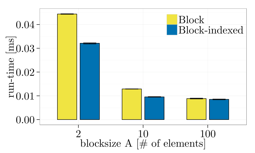
(a) $m=$3.2\text{\,}\mathrm{kB}$$, $2$ nodes

(b) $m=$3.2\text{\,}\mathrm{kB}$$, same node

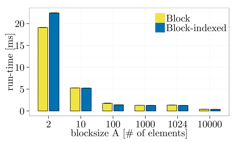
(c) $m=$2.56\text{\,}\mathrm{MB}$$, $2$ nodes

(d) $m=$2.56\text{\,}\mathrm{MB}$$, same node

Figure 102: Block vs. Block-indexed, element datatype: MPI_INT, Ping-pong, Intel MPI-5.1.3.

B.7 Expectation Test 3.2.7 (Sect. 3.2.7)

 

• Alternating, Alternating-indexed

• Ping-pong

 

• Figure 103:   Intel MPI-5.1.3

 

(a) $m=$3.2\text{\,}\mathrm{kB}$$, $2$ nodes

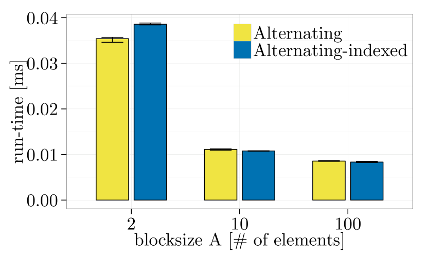
(b) $m=$3.2\text{\,}\mathrm{kB}$$, same node

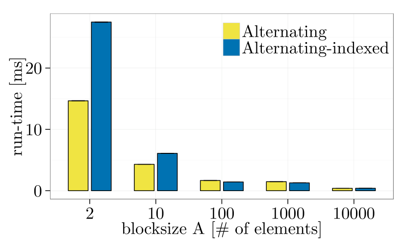
(c) $m=$2.56\text{\,}\mathrm{MB}$$, $2$ nodes

(d) $m=$2.56\text{\,}\mathrm{MB}$$, same node

Figure 103: Alternating vs. Alternating-indexed, element datatype: MPI_INT, Ping-pong, NEC MPI-1.3.1.

B.8 Expectation Test 3.2.8 (Sect. 3.2.8)

 

• Alternating-repeated, Alternating-struct

• Ping-pong

 

• Figure 104:   Intel MPI-5.1.3

 

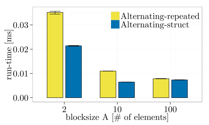
(a) $m=$3.2\text{\,}\mathrm{kB}$$, $2$ nodes

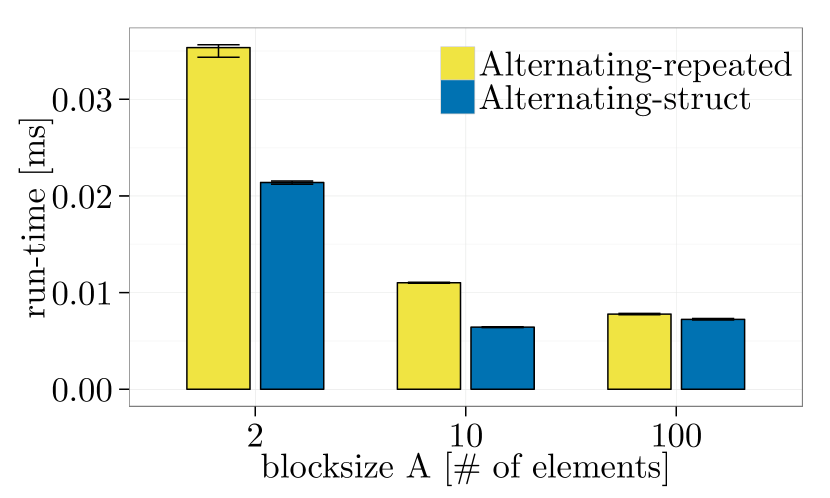
(b) $m=$3.2\text{\,}\mathrm{kB}$$, same node

(c) $m=$2.56\text{\,}\mathrm{MB}$$, $2$ nodes

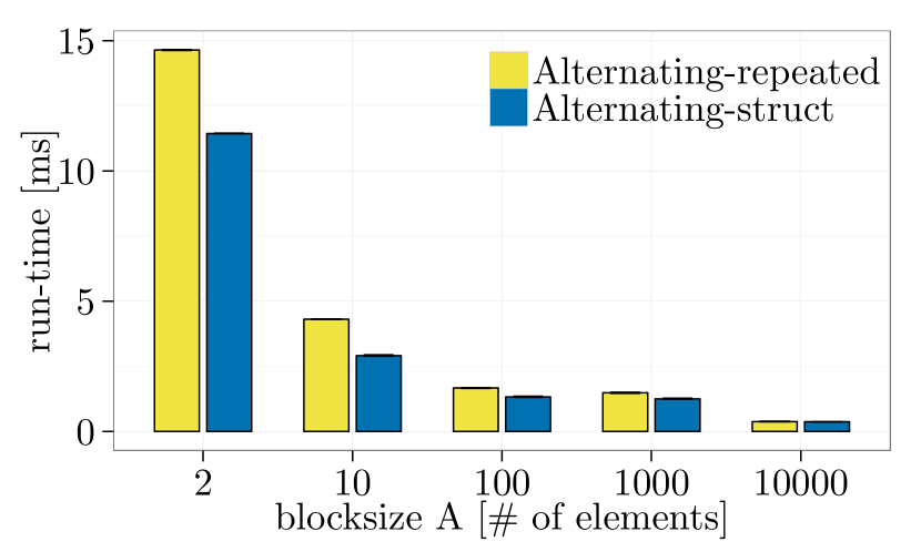
(d) $m=$2.56\text{\,}\mathrm{MB}$$, same node

Figure 104: Alternating-repeated vs. Alternating-struct, element datatype: MPI_INT, Ping-pong, Intel MPI-5.1.3.

B.9 Expectation Test 3.2.3 (Sect. 3.2.3)

 

• Tiled ($AB$), Tiled-struct

• Ping-pong

 

• Figure 105:   Intel MPI-5.1.3

 

(a) $m=$4\text{\,}\mathrm{kB}$$, $2$ nodes

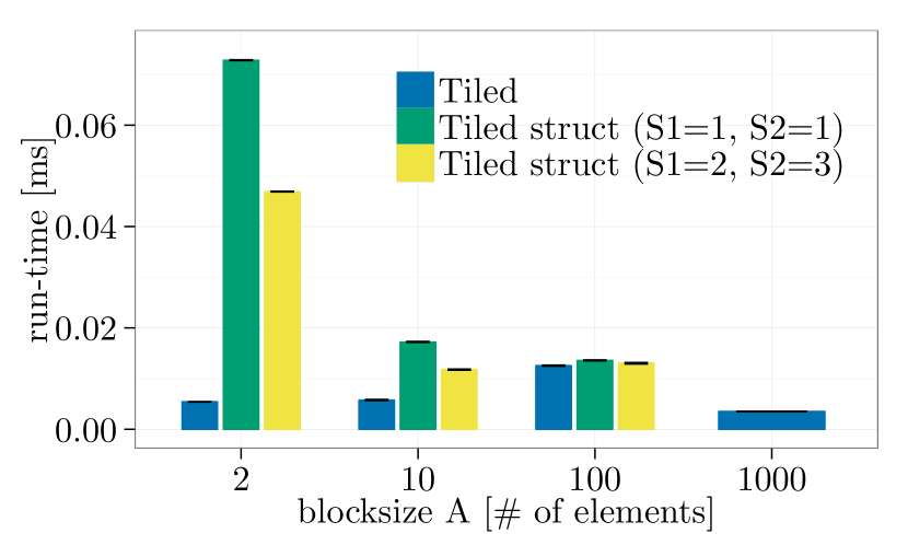
(b) $m=$4\text{\,}\mathrm{kB}$$, same node

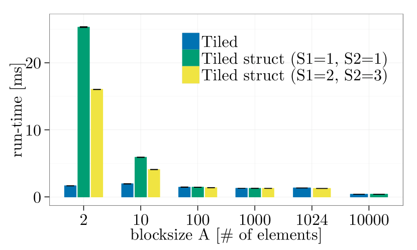
(c) $m=$2.56\text{\,}\mathrm{MB}$$, $2$ nodes

(d) $m=$2.56\text{\,}\mathrm{MB}$$, same node

Figure 105: Tiled ($AB$) vs. Tiled-struct, element datatype: MPI_INT, Ping-pong, Intel MPI-5.1.3.

B.10 Expectation Test 3.2.4 (Sect. 3.2.4)

 

• Tiled ($AB$), Tiled-vector

• Ping-pong

 

• Figure 106:   Intel MPI-5.1.3

 

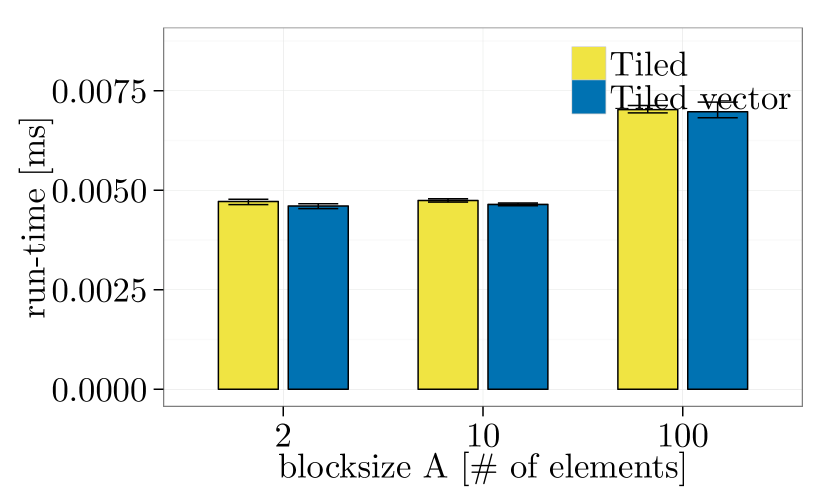
(a) $m=$2\text{\,}\mathrm{kB}$$, $2$ nodes

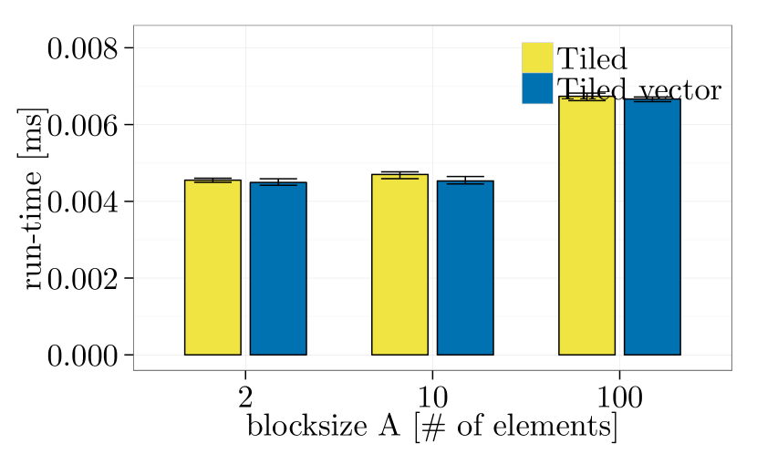
(b) $m=$2\text{\,}\mathrm{kB}$$, same node

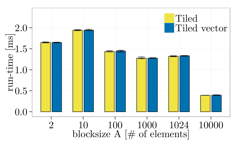
(c) $m=$2.56\text{\,}\mathrm{MB}$$, $2$ nodes

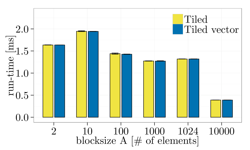
(d) $m=$2.56\text{\,}\mathrm{MB}$$, same node

Figure 106: Tiled ($AB$) vs. Tiled-vector, element datatype: MPI_INT, Ping-pong, Intel MPI-5.1.3.

B.11 Expectation Test 3.2.9 (Sect. 3.2.9)

 

• RowCol-fully-indexed, RowCol-contiguous-and-indexed, RowCol-struct

• Ping-pong

 

• Figure 107:   Intel MPI-5.1.3

 

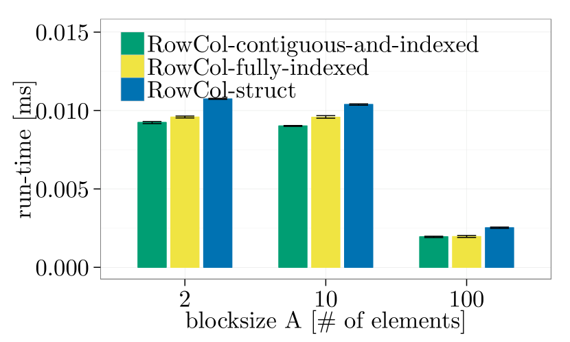
(a) $n=$100$$, $2$ nodes

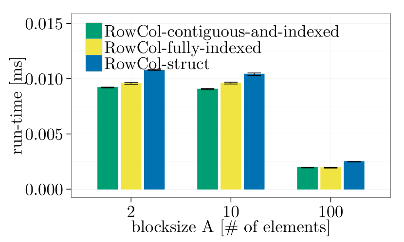
(b) $n=$100$$, same node

(c) $n=$10\,240$$, $2$ nodes

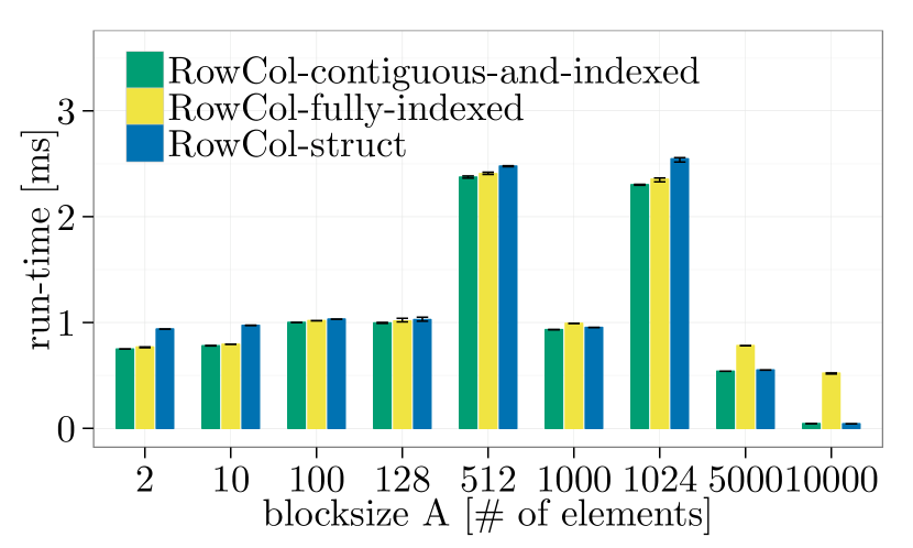
(d) $n=$10\,240$$, same node

Figure 107: RowCol-fully-indexed, RowCol-contiguous-and-indexed, RowCol-struct, element datatype: MPI_INT, extent increases with blocksize $A$, Ping-pong, Intel MPI-5.1.3.

References

- [1] S. Byna, W. D. Gropp, X.-H. Sun, and R. Thakur. Improving the performance of MPI derived datatypes by optimizing memory-access cost. In CLUSTER, pages 412–419, 2003.
- [2] R. Ganian, M. Kalany, S. Szeider, and J. L. Träff. Polynomial-time construction of optimal MPI derived datatype trees. In IPDPS. IEEE Computer Society, 2016.
- [3] W. D. Gropp, T. Hoefler, R. Thakur, and J. L. Träff. Performance expectations and guidelines for MPI derived datatypes: a first analysis. In EuroMPI, pages 150–159. Springer, 2011.
- [4] T. Hoefler and S. Gottlieb. Parallel zero-copy algorithms for fast fourier transform and conjugate gradient using MPI datatypes. In EuroPVM/MPI, pages 132–141, 2010.
- [5] S. Hunold, A. Carpen-Amarie, and J. L. Träff. Reproducible MPI micro-benchmarking isn’t as easy as you think. In EuroMPI/ASIA, pages 69–76. ACM, 2014.
- [6] M. Kalany and J. L. Träff. Efficient, optimal MPI datatype reconstruction for vector and index types. In EuroMPI. ACM, 2015.
- [7] F. Kjolstad, T. Hoefler, and M. Snir. A transformation to convert packing code to compact datatypes for efficient zero-copy data transfer. Technical report, University of Illinois at Urbana-Champain, 2011. Retrieved from http://hdl.handle.net/2142/26452, last visited on 03/01/2016.
- [8] F. Kjolstad, T. Hoefler, and M. Snir. Automatic datatype generation and optimization. In PPoPP, pages 327–328, 2012.
- [9] MPI Forum. MPI: A Message-Passing Interface Standard. Version 3.1, June 4th 2015. www.mpi-forum.org.
- [10] T. Prabhu and W. Gropp. DAME: A runtime-compiled engine for derived datatypes. In EuroMPI, 2015.
- [11] R. Reussner, J. L. Träff, and G. Hunzelmann. A benchmark for MPI derived datatypes. In EuroPVM/MPI, pages 10–17. Springer, 2000.
- [12] R. Ross, N. Miller, and W. D. Gropp. Implementing fast and reusable datatype processing. In EuroPVM/MPI, pages 404–413. Springer, 2003.
- [13] R. B. Ross, R. Latham, W. Gropp, E. L. Lusk, and R. Thakur. Processing MPI datatypes outside MPI. In EuroPVM/MPI, pages 42–53, 2009.
- [14] T. Schneider, R. Gerstenberger, and T. Hoefler. Application-oriented ping-pong benchmarking: how to assess the real communication overheads. Computing, 96(4):279–292, 2014.
- [15] T. Schneider, F. Kjolstad, and T. Hoefler. MPI datatype processing using runtime compilation. In EuroMPI, pages 19–24, 2013.
- [16] M. Schulz, G. Bronevetsky, and B. R. de Supinski. On the performance of transparent MPI piggyback messages. In EuroPVM/MPI, pages 194–201, 2008.
- [17] J. L. Träff. Optimal MPI datatype normalization for vector and index-block types. In EuroMPI/ASIA, pages 33–38. ACM, 2014.
- [18] J. L. Träff, W. D. Gropp, and R. Thakur. Self-consistent MPI performance guidelines. IEEE TPDS, 21(5):698–709, 2010.
- [19] J. L. Träff, R. Hempel, H. Ritzdorf, and F. Zimmermann. Flattening on the fly: efficient handling of MPI derived datatypes. In EuroPVM/MPI, pages 109–116. Springer, 1999.
- [20] J. Wu, P. Wyckoff, and D. K. Panda. High performance implementation of MPI derived datatype communication over InfiniBand. In IPDPS, page 14, 2004.