HERA Mock Observations: Looking for Closure
HERA Memorandum Number 13
May 13, 2016

C.L. Carilli¹¹affiliation: National Radio Astronomy Observatory, P. O. Box 0, Socorro, NM 87801 ²²affiliation: Cavendish laboratory, Cambridge University, UK , P. Sims²²affiliation: Cavendish laboratory, Cambridge University, UK ccarilli@aoc.nrao.edu

Abstract

We investigate the use of closure phase as a method to detect the HI 21cm signal from the neutral IGM during cosmic reionzation. Closure quantities have the unique advantage of being independent of antenna-based calibration terms. We employ realistic, large area sky models from Sims et al. (2016). These include an estimate of the HI 21cm signal generated using 21cm FAST, plus continuum models of both the diffuse Galactic synchrotron emission and the extragalactic point sources. We employ the CASA simulator and adopt the Dillon-Parsons HERA configuration to generate a uv measurement set. We then use AIPS to calculate the closure phases as a function of frequency (’closure spectra’), and python scripts for subsequent analysis. We find that the closure spectra for the HI signal show dramatic structure in frequency, and based on thermal noise alone, the redundant HERA-331 array should detect these fluctuations easily. Comparatively, the frequency structure in the continuum closure spectra is much smoother than that seen in the HI closure spectra. Unfortunately, when the line and continuum signals are combined, the continuum dominates the visibilities at the level of $10^{3}$ to $10^{4}$ , and the line signal is lost. We have investigated fitting and removing smooth curves in frequency to the line plus continuum closure spectra, and find that the continuum itself shows enough structure in frequency in the closure spectra to preclude separation of the continuum and line based on such a process. We have also considered the subtraction of the continuum from the visibilities using a sky model, prior to calculation of the closure spectra. We find that if 99% of the continuum can be subtracted from the visibilities, then the line signal can be seen in the residuals after subsequent smooth curve fitting and removal, although the advantages of such an approach are not clear at this point.

1 Introduction

Detecting the HI 21cm signal from the neutral intergalactic medium during cosmic reionization, and into the preceding dark ages, has been one of the paramount goals of modern astrophysics for the last decade (Morales & Wyithe 2010). However, this task is complicated by the much stronger foreground continuum emission.

A powerful distinguishing property of the foregrounds is that they are dominated by spectrally smooth emission. This is in stark contrast with the 21-cm emission which is expected to fluctuate rapidly in both its spatial and spectral dimensions. A naive solution¹¹1 Without a priori knowledge of the covariance between the foregrounds and the 21-cm signal in the data, independent subtraction of a foreground model from the data prior to estimation of the quantity of interest will produce biased estimates of said quantity. As such, joint estimation of the foregrounds and 21-cm signal is essential for obtaining statistically robust estimates of the 21-cm signal (Sims et al. 2016)., therefore, would be to attempt to removed the foregrounds in the spectral domain by fitting a smoothly varying function (such as a polynomial) in frequency to either the visibilities or the spectral image cubes. However, in his PhD thesis work, A. Datta showed that the chromatic response of an interferometer for very wide field imaging imprints a spectral signature on the visibility data which is impossible to remove using standard continuum subtraction techniques via smooth curve fitting to the visibilty spectra, such as UVLIN in AIPS or uvcontsub in CASA, or point-by-point smooth curve fitting to a spectral image cube. The continuum can still be removed properly, in theory, through a frequency dependent subtraction from the visibilities of an accurate continuum model generated from the data themselves. However, Datta et al. showed that such a subtraction requires remarkably accurate complex gain calibration as a function of frequency (0.1%; Datta et al. 2009; 2010).

These facts have led to consideration of alternative methods for detecting the HI 21cm signal, through ’foreground avoidance’ in delay spectra (Parsons et al. 2012; Morales et al. 2012). The method involves separating HI from continuum in the line of sight vs. sky-plane power-spectral space. In this space, the maximum wave number (or spectral frequency) for flat-spectrum continuum emission due to the chromatic response of a given interferometric baseline is set by the maximum delay of the baseline for sources at the horizon. Hence, the line signal in the line-of-sight direction (frequency) emerges from ’the wedge’ of continuum emission at large wave number (eg. Datta et al. 2010). This avoidance method still requires tight control of the spectral response of other parts of the array, such as the antennas and data transmission system, and/or very accurate calibration of the spectral response (bandpass) with time, to avoid coupling the continuum signal to the line, and hence causing ’bleeding’ of the continuum signal into the EoR window (eg. Pober et al. 2016).

In this memo, we consider an alternate approach for discovering the HI signal using the closure phases of the interferometer. Closure phase results from a simple product of the three visibility pairs from three antennas (Jennison 1958). It was recognized early in the field of radio interferometry that closure quantities are independent of antenna-based phase and amplitude calibration terms. Hence, to the degree that array calibration is separable into antenna-based terms, closure phases are independent of calibration and calibration errors, ie. close quantities are a robust ’observable’ of the true sky signal. This fact was used in early radio interferometry, and in particular, VLBI, when maintaining phase coherence was problematic. Closure quantities are still used extensively in optical interferometry, as well as being the primary diagnostic for antenna-based calibration errors in phase-connected radio interferometers (Perley 1999).

Note that in this memo, the goal is not to characterize the HI 21cm signal from reionization, nor to consider the physical interpretation and its implications for the physics of reionization. These are early days in HI 21cm cosmology, when mere detection of the signal remains paramount. Given the robust nature of closure phase to antenna-based calibration, herein we consider the simple questions: is the HI 21cm line signal from reionization obvious in the closure phase behaviour as a function of frequency? Does the behaviour of the closure phases due to the line signal as a function of frequency differ substantially from that of the continuum? And are the two separable in a simple way?

2 Closure phase

We briefly review the definition of closure phase (see Cornwell & Fomalont 1999).

The van Cittert-Zernike theorem states that the time averaged cross-correlation of the electric field voltages measured at two distinct points in space ( $i,j$ ), which we will call the ’true sky’ visibility, $V_{i,j}^{s}$ , is the Fourier transform of the sky brightness distribution:

V_{i,j,\nu}^{s}(u,v)=\int_{l}\int_{m}I_{\nu}(l,m)e^{-2\pi i(ul+vm)}dldm

where the small angle approximation has been assume, with $u$ and $v$ being orthogonal baseline lengths in units of wavelengths, and $l$ and $m$ as small angle coordinates (direction cosines), measured with respect to the $u$ and $v$ axes. The subscript $\nu$ denotes measurements as a function of frequency, which we will omit heretofore. This quantity is separable into a complex expression of the form:

V_{i,j}^{s}(u,v)=A^{s}_{i,j}e^{i\phi_{i,j}^{s}}

where $A^{s}_{i,j}$ is the true sky visibility amplitude (ie. the amplitude of the sinusoidal fringe on the sky), and $\phi_{i,j}^{s}$ is the phase of the complex visibility (the position of the sinusoidal fringe).

A real interferometer will introduce both thermal noise and complex gain terms, $G$ (ie. amplitude and phase terms due to the instrument response), that will alter the sky visibility to a measured quantity, $V_{i,j}^{m}(u,v)$ :

V_{i,j}^{m}=G_{i}G_{j}^{\ast}V_{i,j}^{s}=a_{i}e^{i\theta_{i}}a_{j}e^{-i\theta_{j}}A^{s}_{i,j}e^{i\phi_{i,j}^{s}}~{}~{}{\rm+~{}noise}

where $\theta_{i}$ is the phase introduced to the visibility by the antenna electronics or optics, and $a_{i}$ is the gain amplitude of the antenna plus electronics. This assumes that the complex gain on a given visibility is separable to antenna-based terms.

From this, we can see that the resulting measured visibility phase is the sum of exponents:

\phi_{i,j}^{m}=\phi_{i,j}^{s}+(\theta_{i}-\theta_{j})~{}~{}{\rm+~{}noise}

The ’bi-spectrum’ or ’triple product’ for an interferometric measurement is defined as:

C_{i,j,k}^{m}=V_{i,j}^{m}V_{j,k}^{m}V_{k,i}^{m}

It is easy to see from the equations above that the phase of this complex measurement, or closure phase, is, again, the sum of exponents:

\phi_{i,j,k}^{m}=\phi_{i,j}^{s}+(\theta_{i}-\theta_{j})+\phi_{j,k}^{s}+(\theta_{j}-\theta_{k})+\phi_{k,i}^{s}+(\theta_{k}-\theta_{i})~{}~{}{\rm+~{}noise}

The antenna based phase terms then cancel in such a triangle, leading to:

\phi_{i,j,k}^{m}=\phi_{i,j,k}^{s}~{}~{}{\rm+~{}noise}

The implication is that the measured closure phase is independent of antenna-based calibration terms, and represents a direct measurement of the true closure phase due to structure on the sky. This fact was recognized early in the field of astronomical interferometry (Jennison 1958), and is still often used in situations where instrumental phase stability and determination of antenna-based calibration terms may be difficult, such as in certain VLBI applications (historically), and optical interferometry (see Thomson, Moran, & Swenson 2007). Note that there is a analogous ’closure amplitude’ based on the combination of four visibility measurements (Cornwell & Fomalont 1999).

Of course, this conclusion relies on the assumption that the phase induced by the system is factorizable into antenna based terms, ie. that the correlator or other aspects of the system do not introduce phase terms that depend on the particular cross correlation for a visibility. Such non-closuing terms are known as ’closure errors’, and remain an important diagnostic on the quality of antenna-based calibration in interferometers (Fomalont & Perley 1999).

3 Sky models, Mock Observations, and Generation of Closure Phase

The HI 21cm signal was generated using 21cmFAST (Mesinger et al. 2011). In order to investigate very wide field effects, the input model is 45^o across, generated by tiling a series of line cubes with structure based on the excursion set analysis for the IGM during cosmic reionization (Sims et al. 2016). A very wide-band cube was generated, from roughly 100MHz to 200MHz, with 0.21MHz channels. From this, we selected an 8MHz band at $z=10$ , or 130MHz for the HI line, and for which the IGM in the model has a mean neutral fraction of 0.5.

The continuum model corresponds to a higher Galactic latiture field ( $b=-78^{o}$ ). This model is also very wide field (45^o), and includes models for both the Extragalactic point sources, and the Galactic diffuse synchrotron emission based on existing low frequency observations but extrapolated to smaller scales in a statistically defensible manner (Sims et al. 2016).

The input sky model is in FITS image cube format, in units of Jy pixel^-1, with a pixel size of $85"$ (converted from the original Kelvin brightness unit). Images resulting from these models are presented in Carilli & Sims (2016). The model is folded through the CASA simulator, SIMOBSERVE, using the Dillon-Parsons (2016) ’split core’ array for HERA-350, although we only use the shortest baselines for the analysis herein. We then export the visibility measurement set in FITS format, and load into AIPS. Closure phases as a function of frequency (’closure spectra’), are then generated using the AIPS task CLPLT, in ascii format. Further analysis is done in Python.

The hexagonal configuration has a distinct advantage for closure phase consideration due to the many redundant triangles. We assume the number of independent triangles based on the Dillon & Parsons HERA-331 ’split core’ configuration. In this memo, we consider only the three shortest equilateral triangles in the array, ie. triangles of 1, 2, and 3 times the grid spacing of 14.6m. There are roughly 75 of each triangle in the array (although there may be a better way of combining baselines in the configurtation that improves signal to noise).

Under these assumptions, we calculate the signal-to-noise in the measurements based on thermal noise. We assume a total integration time of 100 hours. The transit time for the 10^o primary beam is 40min, so this would take 150days. We adopt a channel width of 0.21MHz and system performance as per de Boer et al. (2016), leading to an rms per visibility of 12mJy. The typical HI signal amplitude on the short baselines $\sim 4$ mJy. Hence, the S/N per visibility phase measurement is $\sim 0.33$ . This improves by a factor root(3/2) for the closure triangle (I think), implying a signal-to-noise for each closure triangle of $\sim 0.40$ . Summing the 75 redundant triangles then leads to a signal-to-noise of $\sim 3.5$ per closure triangle length. Adopting the analysis of Wrobel & Walker (1999) for phase noise as a function of signal-to-noise, leads to a phase error of $\sigma\sim 17^{o}$ per channel in the closure spectra.

4 Results

We consider the HI and continuum closure spectra separately, in order to investigate their relative behaviour. We then consider the closure spectra for the summed line and continuum emission, and methods to extract the line signature in the presence of the much stronger continuum.

4.1 Line signal only

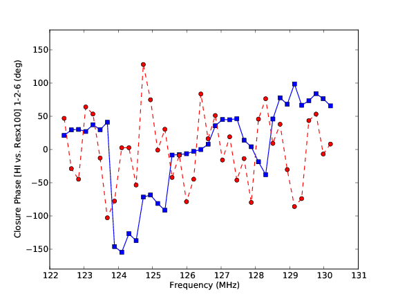
Figure 1 shows the frequency dependence of the closure phase for the three different triangles. The line signal shows large fluctuations across the spectrum. This is consistent with the large changes in sky signal across the band, ie. substantially changing structure with frequency on scales of the bandwidth and spatial resolution of the baseline. Note that there is a $\pm 180^{o}$ ambiguity inherent in phase measurements, leading to apparent ’jumps’ at high positive or negative values. Some of these have been rectified as logic dictates.

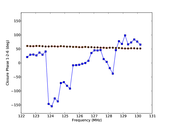
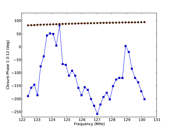
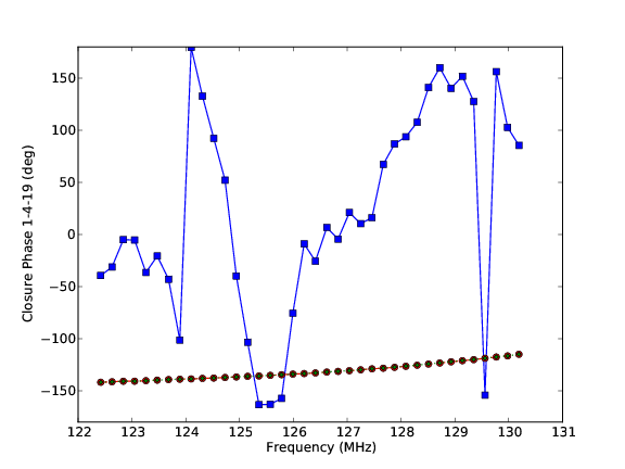
Refer to caption — Figure 1: The closure phase spectra for the three smallest equilateral antenna triangles in HERA. The blue curves are the closure phases for just the HI 21cm signal. The expected thermal noise in each spectral channel based on the signal-to-noise for the HI signal is $\sigma\sim 17^{o}$ , after redundancy is applied (Wrobel & Walker 1999).The green curve shows the values for the continuum foregrounds only, while the red curves show the values for the sum of the continuum and HI line signal. Note that, since the continuum foregrounds dominate the signal by a factor of $>10^{3}$ , the green and red curves are indistiguishable on this scale.

4.2 Adding the Continuum

Figure 1 also includes the closure phase vs. frequency curves for the continuum model, and the continuum plus line models. The frequency structure for the continuum emission is much smoother than that seen for the line signal, although not completely structure-less. Note that on the baselines in question (6 wavelengths to 20 wavelengths = 14.6m to 44m), the continuum foreground visibility amplitudes are $\sim 10$ Jy to 60Jy, while the HI 21cm line visibilities are $\sim 4$ mJy. Hence, the continuum foregrounds dominate the signal by a factor of $\sim 10^{3}$ to $10^{4}$ (in terms of Jansky per visibility), and the green and red curves are indistiguishable on this scale.

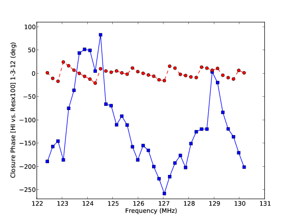
Fig 2 shows the continuum closure spectra for the three triangles. In this case, a mean value has been removed, in order to enhance the scale. The shortest triangle shows the most frequency structure, while the longer triangles show smoother behaviour of closure phase with frequency.

The one hopeful result is that the continuum closure spectra appear much smoother with frequency than the line spectra. But are they smooth enough to remove a smooth curve in frequency in order to recover the line signature?

We note that we cannot rule-out the possibility that the closure phase structure of the continuum emission is an artefact of our sky models and mock-observation process. However, that would be wishful thinking.

4.3 Line plus continuum with a smooth spectral model removed

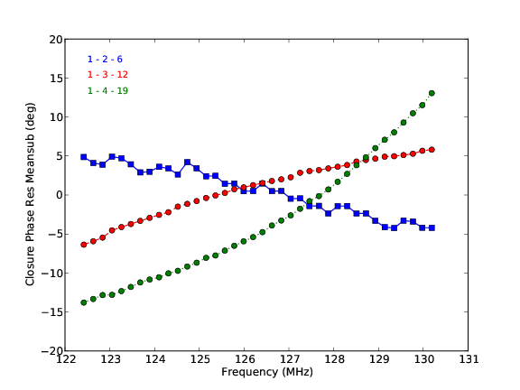
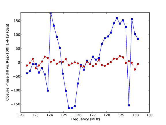
We consider the possibility of removing the continuum via low order polynomial fitting in frequency. Fig 3 shows the results of the closure spectra for a summed line plus continuum model, but with a third order polynomial fit in frequency and subtracted. The residuals are then multiplied by 100. Also included are the HI-only closure spectra. The idea is to look for structure in the residual corresponding to the contribution of the line signal.

We have performed this analysis for all three closure triangle lengths. The shortest closure triangle shows the largest frequency dependent structure of the continuum. This may be due to ’small number statistics’, ie. that on the shortest baselines we only have a few independent resolution elements over the primary beam. The residuals become smaller on longer baselines, due to the iherently smoother continuum closure spectra. However, comparing to the expected HI closure spectra, there is still no sign of the HI signal.

Keep in mind that polynomial fitting does not take into consideration possible covariance between the 21-cm signal and the spectral structure in the foreground model, and can potentially also remove some of the HI signal. As such, simultaneous estimation of the 21-cm closure signal and our foreground model would be much more effective for recovering unbiased estimates, as has been shown in the general Bayesain approach to HI 21cm power spectral estimation by Sims et al. (2016) and Lentati et al. (2016).

4.4 Removal of 99% of the continuum

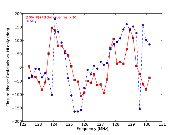
Lastly, we ask the question: what fraction of the continuum needs to be removed in order to recover the line signal? Figure 4 shows the results assuming 99% of the continuum can be removed via imaging and subtraction of the resulting sky model from the visibilities as a function of frequency. We only consider one triangle, as representative.

The red curve shows the residual closure spectrum after continuum subtraction from the visibilities, and subsequent third order polynomial fitting and removal in frequency for the closure spectrum. The residuals are then multiplied by 30. Also shown is the HI-only spectrum in blue.

In this case, there is an apparent correlation between the expected HI signal, and the residuals after polynomial fitting. The broad structures are generally reproduced, with some gradual deviation due to the assumed 3rd order fit.

We should point out that such a process may obviate the need for a closure analysis, since it assumes that excellent calibration as a funciton of frequency will be obtained to generate the model images for subtraction.

5 Conclusions

We have considered closure phase in the context of detecting the HI 21cm signal from the neutral IGM. The good news is that the closure spectra for the HI signal show dramatic structure in frequency, and based on thermal noise alone, the redundant HERA-331 array should detect these fluctuations easily. Also good news is that the frequency structure in the continuum closure spectra is much smoother than that seen in the HI closure spectra.

The bad news remains the extreme brightness difference between the continuum and line emission. The continuum dominates the visibilities at the level of $10^{3}$ to $10^{4}$ . We have investigated smooth-curve fitting and removal to the line plus continuum closure spectra, and find that the continuum itself shows enough structure in frequency in the closure spectra to preclude separation of the continuum and line based on such smooth-curve fitting and removal.

We have also considered the possibility of subtraction of the continuum using a sky model (derived from the observations), prior to calculation of the closure spectra. We find that if 99% of the continuum can be subtracted from the visibilities prior to calculation of closure spectra, then the line signal can be seen in the residuals after subsequent smooth curve fitting and removal. Of course, if we can calibrate the data to the level required for sky model generation and subtraction, the need for a closure analysis becomes potentially redundant.

We can speculate that the natural chromatic response of the interferometer is causing, in part, the spectral structure in the closue spectra of the continuum. In this case, there may be a ’wedge-like’ approach that could be used, in which the statistics of the frequency-dependent structure in the closure spectra (eg. a closure power spectrum), is signficantly different for the line vs. the continuum, thereby allowing for isolation of the line signal in some power-spectral domain.

Similarly, we will explore a Bayesian approach to closure phase analysis, in which any covariance between the foregrounds and the 21-cm signal in the data is dealt with explicitly through joint estimation of the foregrounds and 21-cm signatures. The advantage of employing closure quantities over the current visibility-based analyses remains the robustness of the measured closure quantities to calibration and calibration errors.

References

Jennison 1958, MNRAS, 118, 276

Carilli, C. & Sims, P. 2016, HERA Memo. No. 12

Cornwell & Fomalont 1999, in Synthesis Imaging in Radio Astronomy II,’ eds. G. B. Taylor, C. L. Carilli, and R. A. Perley. ASP 180, 1999, p. 187

de Boer, D. et al. 2016, PASP, submitted

Datta, A., Bowman, J. , Carilli, C. 2010, ApJ, 724, 526

Datta, A., Bhatnagar, S. , Carilli, C. 2009, ApJ, 703, 185

Dillon, J., & Parsons, A. 2016, ApJ, submitted (arXiv:1602.06259

Lentati, L. et al. 2016, MNRAS, submitted

Mesinger, A. & Furlanetto, S., Cen, R. 2011, MNRAS, 411, 955

Morales, M. et al. 2012, ApJ, 752, 137

Morales, K. & Wyithe, S. 2010, ARAA, 48, 127

Parsons, A. et al. 2012, apJ, 756, 165

Perley, R. & Fomalont, E. 1999, in Synthesis Imaging in Radio Astronomy II,’ eds. G. B. Taylor, C. L. Carilli, and R. A. Perley. ASP 180, 1999, p. 79

Perley, R. 1999, in Synthesis Imaging in Radio Astronomy II,’ eds. G. B. Taylor, C. L. Carilli, and R. A. Perley. ASP 180, 1999, p. 275

Pober, J. et al. 2016, ApJ, 819, 8

Sims, P. et al. 2016, MNRAS, submitted.

Thompson, A.R., Moran, J., Swenson, G. 2007, Interferometry and Synthesis in Radio Astronomy, John Wiley & Sons, 2007.

Wrobel, J. & Walker, R.C. 1999, in Synthesis Imaging in Radio Astronomy II,’ eds. G. B. Taylor, C. L. Carilli, and R. A. Perley. ASP 180, 1999, p. 171

HERA Mock Observations: Looking for Closure HERA Memorandum Number 13 May 13, 2016