Microscopic Description of Diffractive Deuteron Breakup
by ${}^{3}\text{He}$ Nuclei

V. I. Kovalchuk

Department of Physics, Taras Shevchenko National University, Kiev 01033, Ukraine

PACS: 24.10.Ht, 24.50.+g, 25.10.+s

1. Introduction

Investigations between collisions of light nuclei treated as composite particles are an important source of information about the microscopic structure of these nuclei and about mechanisms of nuclear reactions proceeding under specific kinematical conditions. While one can still describe reactions involving three or four particles on the basis of a rigorous theory (for example, by invoking, respectively, the formalism of Faddeev equations or the formalism of Faddeev-Yakubovsky equations), a description of the interaction between nuclear systems featuring a greater number of particles already requires employing approximate methods.

The diffraction model of multiparticle collisions [1], which admits the inclusion of a microscopic description of nucleon-density distributions, nucleon-nucleon phase shifts, and the corresponding profile functions, can be considered as one such approach. This permits minimizing the number of adjustable parameters, whereby one can obtain a quantitative description of relevant experimental data and verify the model itself and its applicability boundaries for the kinematics of the reaction being considered. By and large, the application of this approach complicates somewhat the formalism used: for example, the integrands in the scattering amplitude develop a dependence on multiple integrals. As will be shown below, however, the ultimate expression for the reaction amplitude can be reduced to an algebraic expression – multiple sums involving elementary functions – if Gaussian functions are used as integrands. Here, Gaussian functions can be used as basis functions in expansions of both wave functions for colliding nuclei (variational problem) and arbitrary profile functions. It is noteworthy that a similar procedure was extensively employed in the variational approach in describing bound states of light nuclei [2, 3, 4], in parametrizations of ground-state charge densities of nuclei [5, 6], and in the problems of scattering [7] and deuteron stripping [8]. This makes it possible to calculate analytically respective phase shifts and form factors.

We note that, in [9], the diffraction model of multiple scattering was already used to describe the breakup reaction ${}^{3}\text{H}(d,p)n{{}^{3}}\text{H}$. The approach proposed in [9] is formally microscopic because it is based on nucleon-nucleon interactions, but the authors of that study used profile functions including free parameters and replaced the deuteron wave function by a simple Gaussian function, which do not reproduce the asymptotic behavior of the nuclear density at large nucleon-nucleon distances. Since the cross sections for deuteron-breakup reactions (in just the same way as those for deuteron-stripping reactions) are sensitive to the behavior of the deuteron wave function in the region of its tail [10], one can consider the results obtained in [9] as quite approximate ones.

In the present study, exclusive spectra for deuteron breakup by ${}^{3}\text{He}$ nuclei at the energy of 89.4 MeV [11] were chosen as the object of our analysis based on the microscopic diffraction nuclear model. Here, we do not take into account Coulomb interaction because, in our case, the barrier height is approximately equal to 1.5 MeV, so that the emission angles of particles exceed $20^{\circ}$. We do not take into account particle spins either.

2. Formalism

Let us introduce the coordinate frame in which the coordinate origin coincides with the center of mass of the target nucleus (deuteron), while the positive direction of the $z$-axis coincides in direction with the projectile momentum ${\bf k}$ (see Fig. 1).

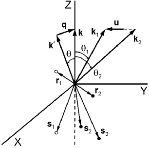
Figure 1: Coordinate frame used in calculating the amplitude for deuteron breakup by ${{}^{3}}\text{He}$ nuclei. The open and closed circles represent neutrons and protons, respectively.

In this coordinate frame, the amplitude for diffractive deuteron breakup by ${{}^{3}}\text{He}$ nuclei can be represented, according to [1], in the form

$$F({\bf q,u})=\frac{ik}{2\pi}\int d{\bf b}\exp(i{\bf qb})\int d{\bm{\tau}}\Phi_{\bf u}^{*}(\bm{\tau})\sum_{\ell=1}^{3}\Bigl{(}1-\prod_{j=1}^{2}\bigl{[}1-\omega_{j\ell}(b_{j\ell})\bigr{]}\Bigr{)}\Phi_{0}(\bm{\tau}),$$ (1)

where ${{\bf q}={\bf k}-{\bf k}^{\prime}}$ is the momentum transfer; $k(k^{\prime})$ is the incident-nucleus (scattered nucleus) momentum; ${{\bf u}=({\bf k}_{1}-{\bf k}_{2})/2}$ is the relative momentum deuteron-breakup products; ${\bf b}=({\bf s}_{1}+{\bf s}_{2}+{\bf s}_{3})_{\perp}/3$ is the projection of the vector of the ${{}^{3}}\text{He}$-nucleus center of mass onto the $xy$-plane; $b_{j\ell}=|{\bf b}_{j\ell}|$ (where ${\bf b}_{j\ell}=({\bf r}_{j}-{\bf s}_{\ell})_{\perp}$ is the impact-parameter vector lying in the $xy$-plane and corresponding to a collision between the $j{\text{th}}$ deuteron nucleon and the $\ell{\text{th}}$ nucleon of the ${{}^{3}}\text{He}$ nucleus); and $\bm{\tau}$ is the set of coordinates that describe the intrinsic degrees of freedom of nucleons belonging to the deuteron and ${{}^{3}}\text{He}$ nucleus involved. Further, the quantities $\Phi_{0}$ and $\Phi_{\bf u}$ in expression (1) are the wave functions that describe the system under study, respectively, before and after the collision event; that is,

$$\Phi_{0,{\bf u}}(\bm{\tau})=\psi_{0}({\bf s})\varphi_{0,{\bf u}}(\bf r),$$ (2)

where $\psi_{0}({\bf s})$ is the ground-state wave function for the ${{}^{3}}\text{He}$ nucleus, $\varphi_{0}(\bf r)$ is the ground-state deuteron wave function, and the function $\varphi_{{\bf u}}(\bf r)$ describes the relative motion of the neutron and proton that originated from deuteron breakup.

Since $d{\bf b}=d^{(2)}{\bf b}$, $d{\bm{\tau}}=d^{(3)}{\bf s}\,d^{(3)}{\bf r}$, expression (1) is formally an eight-dimensi-onal integral. A direct calculation of such integrals presents a difficult challenge from the point of view of convergence of quadrature sums and computational errors, but, upon expanding the integrands in terms of a Gaussian basis, the amplitude in (1) admits an analytic evaluation.

We now recast expression (1) into the form

$$F({\bf q,u})=\frac{ik}{2\pi}\int d{\bf b}\exp(i{\bf qb})\int d{\bf s}\,d{\bf r}\,\rho(s)\varphi_{0}({\bf r})\varphi_{{\bf u}}^{*}({\bf r})\sum_{\ell=1}^{3}\Bigl{(}1-\prod_{j=1}^{2}\bigl{[}1-\omega_{j\ell}(b_{j\ell})\bigr{]}\Bigr{)},$$ (3)

where $\rho(s)=\psi_{0}({\bf s})\psi_{0}^{*}({\bf s})$ is the normalized (to unity) nucleon-density distribution in the ${{}^{3}}\text{He}$ nucleus and $s^{2}=({\bf s}_{1}-{\bf s}_{2})^{2}+({\bf s}_{2}-{\bf s}_{3})^{2}+({\bf s}_{1}-{\bf s}_{3})^{2}$. In order to evaluate the integrals in expression (3), we take the integrands $\rho(s)$, $\varphi_{0}(\bf r)$, and $\varphi_{{\bf u}}({\bf r})$ in the form

$$\rho(s)=\sum_{n=1}^{K}a_{n}\exp(-b_{n}s^{2}),$$ (4)

$$\varphi_{0}({\bf r})=\sum_{n=1}^{K}c_{n}\exp(-d_{n}r^{2}),\quad r^{2}={\bf r}^{2}=|{\bf r}_{1}-{\bf r}_{2}|^{2},$$ (5)

$$\varphi_{{\bf u}}({\bf r})=\exp(i{\bf u}{\bf r})-\sqrt{8}\exp\Bigl{(}-\frac{u^{2}}{4\lambda}-\lambda r^{2}\Bigr{)}.$$ (6)

The functions in (4) and (5) are the solutions that the use of a Gaussian basis makes it possible to obtain for the variational problems of the bound states of the ${{}^{3}}\text{He}$ nucleus and the deuteron for the K2 nucleon-nucleon potential [3, 4]. At $K=10$, the two functions in question faithfully reproduce the experimental values of the binding energy and root-mean-square radii of these nuclei and have a correct asymptotic behavior at short and long nucleon–nucleon distances. In expression (5), $\lambda$ is the harmonic-oscillator-potential parameter chosen in such a way as to reproduce the deuteron binding energy in solving the respective Schrödinger equation for the bound state of the neutron and proton. The authors of [12] indicate that the wave function (6) is not a solution of the Schrödinger equation for a continuum, nor does it have an asymptotic behavior at infinity in the form of a converging spherical wave; it does not satisfy the orthonormalization condition either:

$$\int\varphi_{{\bf u}^{\prime}}^{*}({\bf r})\varphi_{{\bf u}}({\bf r})d{\bf r}=(2\pi)^{3}\delta({\bf u}^{\prime}-{\bf u}).$$ (7)

However, as was indicated in [13, 14], the results of calculations for the deuteron-breakup cross sections exhibit by and large a low sensitivity to the choice of wave functions describing the relative motion of the neutron and proton in the final S-wave state. In such problems, one usually chooses $\varphi_{{\bf u}}({\bf r})$ in the form (6) for the sake of convenience, and this sometimes makes it possible to calculate form factors and reaction amplitudes analytically.

The nucleon–nucleon profile functions $\omega_{j\ell}$ in (3) were calculated in the high-energy approximation [15]; that is,

$$\omega_{j\ell}(b_{j\ell})=1-\exp(-\phi_{j\ell}(b_{j\ell})),$$ (8)

where $\phi_{j\ell}$ is is the phase shift for the scattering of the $j{\text{th}}$ deuteron nucleon by the $\ell{\text{th}}$ nucleon of the ${{}^{3}}\text{He}$ nucleus:

$$\phi_{j\ell}(b_{j\ell})=-\frac{1}{v}\int_{-\infty}^{\infty}dz\,W\Bigl{(}\sqrt{b_{j\ell}^{2}+z^{2}}\Bigr{)}.$$ (9)

Here, $v$ is the speed of the incident nucleon and $W(r)$ is the imaginary part of the nucleon–nucleon potential.

Within the double-folding model, the eikonal phase shift in (9) can be calculated analytically [16]. The result has the form

$$\phi_{j\ell}(b_{j\ell})=N_{W}\frac{\pi^{2}\,\bar{\sigma}_{j\ell}\,a_{j}^{3}\,a_{\ell}^{3}\,\rho_{j}(0)\,\rho_{\ell}(0)}{a_{j}^{2}+a_{\ell}^{2}+r_{0}^{2}}\exp\Bigl{[}-\frac{b_{j\ell}^{2}}{a_{j}^{2}+a_{\ell}^{2}+r_{0}^{2}}\Bigr{]},$$ (10)

where $N_{W}$ is the normalization parameter of the potential $W(r)$ and $\bar{\sigma}_{j\ell}$ is the isotopically averaged total cross section for nucleon–nucleon interaction. For various type of colliding nucleons, we have $\bar{\sigma}_{j\ell}=\sigma_{nn}=\sigma_{pp}$ or $\bar{\sigma}_{j\ell}=\sigma_{np}=\sigma_{pn}$. The cross sections $\sigma_{pp}$ and $\sigma_{pn}$ are described in terms of phenomenological dependences [16, 17].

Expression (10) was derived in [16] under the assumption that the intranuclear-nucleon-density distribution $\rho_{j,\ell}(r)$ and the nucleon–nucleon interaction amplitude $f_{j\ell}(b)$ are defined in terms of Gaussian functions as

$$\rho_{j,\ell}(r)=\rho_{j,\ell}(0)\exp(-r^{2}/a_{j,\ell}^{2}),\quad f_{j\ell}(b)=(\pi r_{0}^{2})^{-1}\exp(-b^{2}/r_{0}^{2}).$$ (11)

Considering that $\rho_{j}(0)\!=\!\rho_{\ell}(0)\!=\!(a\sqrt{\pi})^{-3}$ and $a_{j}\!=\!a_{\ell}\!=\!a\!=r_{0}\!=\!\sqrt{2/3}\,R_{NN}$ [18], where $R^{2}_{NN}\cong 0,65\,\,\text{fm}^{2}$ is the root-mean-square range of nucleon–nucleon interaction, we recast expression (10) into the form

$$\phi_{j\ell}(b_{j\ell})=N_{W}\frac{\bar{\sigma}_{j\ell}}{3\pi a^{2}}\exp\Bigl{[}-\frac{b_{j\ell}^{2}}{3a^{2}}\Bigr{]}.$$ (12)

Expression (12) was directly used to calculate the profile functions (8), which were thereupon expanded in terms of a Gaussian basis as

$$\omega_{j\ell}(b_{j\ell})=\sum_{n=1}^{K}\alpha_{n}^{(j\ell)}\exp(-\beta_{n}^{(j\ell)}b_{j\ell}^{2}),\quad j\ell=pp,pn.$$ (13)

Taking into account the nucleon content of colliding nuclei, we spell out the sum in (3) as

$$\sum_{\ell=1}^{3}\Bigl{(}1-\prod_{j=1}^{2}\bigl{[}1-\omega_{j\ell}\bigr{]}\Bigr{)}=-3(\omega_{pp}+\omega_{pn}-\omega_{pp}\,\omega_{pn}).$$ (14)

Evaluating the integral in expression (3) with the functions (4)–(6), (13), and with allowance for relation (14), we obtain

$$F({\bf q,u})=-\frac{i\pi^{4}\sqrt{\pi}k}{4\sqrt{3}}\bigl{(}\Omega^{(1)}(q)-\Omega^{(2)}(q)\bigr{)}f({\bf q,u}),$$ (15)

where

$$\Omega^{(1)}(q)=\sum_{i=1}^{K}\left(\frac{\alpha_{i}^{(pp)}}{\beta_{i}^{(pp)}}\exp\left[-\frac{q^{2}}{4\beta_{i}^{(pp)}}\right]+\frac{\alpha_{i}^{(pn)}}{\beta_{i}^{(pn)}}\exp\left[-\frac{q^{2}}{4\beta_{i}^{(pn)}}\right]\right),$$ (16)

$$\Omega^{(2)}(q)=\sum_{i=1}^{K}\sum_{j=1}^{K}\frac{\alpha_{i}^{(pp)}\alpha_{j}^{(pn)}}{\beta_{i}^{(pp)}+\beta_{j}^{(pn)}}\exp\left[-\frac{q^{2}}{4\bigl{(}\beta_{i}^{(pp)}+\beta_{j}^{(pn)}\bigr{)}}\right],$$ (17)

$$f({\bf q,u})=\sum_{i=1}^{K}\sum_{j=1}^{K}\frac{a_{i}}{b_{i}^{3/2}}\frac{c_{j}}{d_{j}^{3/2}}\exp\left[-\frac{q^{2}}{18b_{i}}\right]\exp\left[-\frac{u_{z}^{2}}{4d_{j}}\right]$$

$$\times\left(\exp\left[-\frac{(u_{\perp}+q/2)^{2}}{4d_{j}}\right]+\exp\left[-\frac{(u_{\perp}-q/2)^{2}}{4d_{j}}\right]-2\exp\left[-\frac{u_{\perp}^{2}}{4d_{j}}+\frac{q^{2}}{16\bigl{(}d_{j}+\lambda\bigr{)}}\right]\right).$$ (18)

Here, $u^{2}=u^{2}_{\perp}+u^{2}_{z}$, with ${\bf u}_{\perp}$ lying in the impact–parameter $xy$-plane. Equations (15)–(18) were obtained for the case where the vectors ${\bf q}$ and ${\bf u}$ are coplanar, which is valid for the geometry of the experiment reported in [11] and analyzed below.

3. Results of calculations and their comparison with experimental data

In [19], where the problem of deuteron breakup by medium-mass and heavy nuclei was examined, an expression for the exclusive deuteron-breakup cross section was obtained in the form

$$\sigma(\theta_{1},\theta_{2},E_{2})=\frac{d^{3}\sigma}{d\Omega_{1}d\Omega_{2}dE_{2}}=\frac{m^{5/2}E_{1}E_{2}}{2k^{2}\sqrt{E_{1}+E_{2}+\epsilon}}|F({\bf q},{\bf u})|^{2},$$ (19)

where $m$ is the nucleon mass; $E_{1}$ and $E_{2}$ are the energies of, respectively, the neutron and the proton scattered into the respective solid-angle elements $d\Omega_{1}$ and $d\Omega_{2}$; and $\epsilon$ is the deuteron binding energy.

The detecting system used in [11] recorded a ${{}^{3}}\text{He}$ nucleus scattered at an angle $\theta$ and one deuteron-breakup product (proton), to which the angle $\theta_{2}$ and the energy $E_{2}$ correspond. These three kinematical variables determine the differential cross section $\sigma(\theta,\theta_{2},E_{2})$ observed in the experiment under discussion. If the neutron (as a deuteron-breakup product) were detected instead of the ${{}^{3}}\text{He}$ scattered nucleus, we would have had the relation $\sigma(\theta,\theta_{2},E_{2})=\sigma(\theta_{1},\theta_{2},E_{2})$. Therefore, experimental spectra from [11] can be described by expression (19) under the condition the emission angles $\theta_{1}$ and $\theta_{2}$ for the neutron and proton and their respective energies $E_{1}$ and $E_{2}$ are known.

The experiment reported in [11] was performed in coplanar geometry – that is, the vectors ${\bf k}$, ${\bf k}^{\prime}$, ${\bf q}$, and ${\bf k}_{2}$ lay in the the scattering plane (see Fig. 1). From the momentum-conservation law ${\bf k}={\bf k}^{\prime}+{\bf k}_{1}+{\bf k}_{2}$, it follows that the vector ${\bf k}_{1}$ also lies in this plane, and so does therefore the vector ${\bf u}=({\bf k}_{1}-{\bf k}_{2})/2$. The unknown quantities $\theta_{1}$ and $E_{1}$ can be found from a set of nonlinear equations that is obtained by supplementing the momentum-conservation law with the energy-conservation law

$$\left\{{\begin{array}[]{*{20}l}{q=q_{\perp}=k^{\prime}\sin{\theta}}=k_{1}\sin{\theta_{1}}+k_{2}\sin{\theta_{2}},\\ {k=k^{\prime}\cos{\theta}+k_{1}\cos{\theta_{1}}+k_{2}\cos{\theta_{2}},}\\ {E=E^{\prime}+E_{1}+E_{2}+\epsilon.}\\ \end{array}}\right.$$ (20)

The set of Eqs. (20) is solved numerically – the sought values of $E^{\prime}$, $E_{1}$, and $\theta_{1}$ are found for each set of known values of $E$, $\theta$, $E_{2}$, and $\theta_{2}$.

That detector in [11] which recorded the ${{}^{3}}\text{He}$ scattered nucleus was arranged at a fixed angle of $\theta=20^{\circ}$, and emitted protons were detected in the angular range of $\theta_{2}=20^{\circ}\!\div\!60^{\circ}$. By way of example, Fig. 2 shows the dependences $q(E_{2})$ and $u(E_{2})$ calculated at an angle of $\theta_{2}=20^{\circ}$ (see Fig. 2a) and the values of the minima $q_{\text{min}}$ and $u_{\text{min}}$ versus the angle $\theta_{2}$ (Fig. 2b).

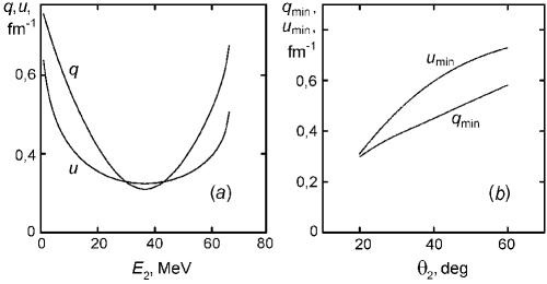
Figure 2: Results of solving the set of Eqs. (20) at $\theta=20^{\circ}$: $(\textit{a})$ $q$ and $u$ versus the proton energy $E_{2}$ at $\theta_{2}=20^{\circ}$ and $(\textit{b})$ values of $q_{\text{min}}$ and $u_{\text{min}}$ versus the angle $\theta_{2}$.

This figure shows that the dependences $q(E_{2})$ and $u(E_{2})$ pass through a minimum at specific values of the proton energy $E_{2}$; a similar behavior of the quantities $q$ and $u$ is also characteristic of the remaining values of the angle $\theta_{2}$ that were preset in the experiment reported in [11]. With increasing $\theta_{2}$, the proton energy at which $q(E_{2})$ and $u(E_{2})$ reach a minimum decreases (not shown in Fig. 2), while the values of $q_{\text{min}}$ and $u_{\text{min}}$ themselves increase.

Figure 3 shows the calculated cross sections (19). In this figure, the solid curves were calculated with the amplitude in (15), the normalization parameter of the imaginary part of the high-energy nucleon–nucleon potential being set to $N_{W}=0.13$ $(\theta_{2}=20^{\circ})$; 0.21 $(25^{\circ})$; 0.32 $(30^{\circ})$; 0.53 $(35^{\circ})$; 0.89 $(40^{\circ})$; 0.98 $(45^{\circ})$; 1.0 $(50^{\circ})$; and 1.0 $(55^{\circ})$.

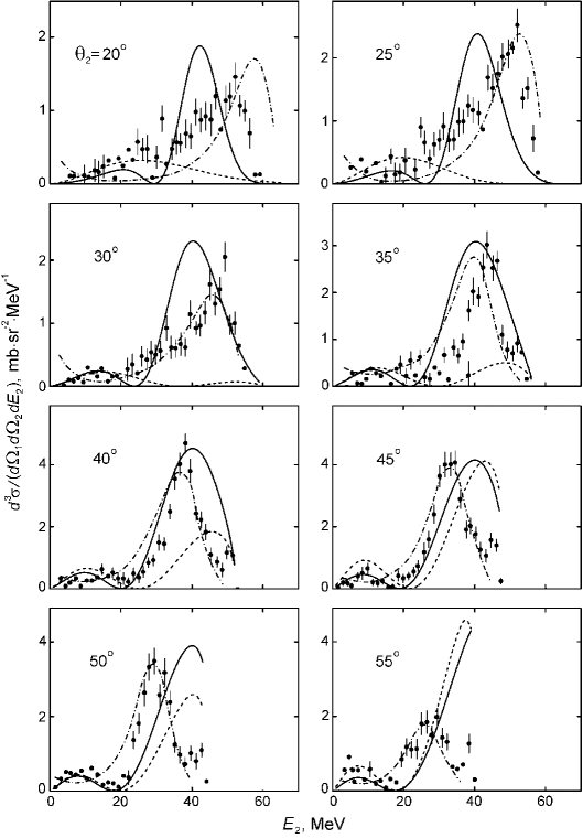
Figure 3: Energy distributions of protons from the reaction ${{}^{2}}\text{H}({{}^{3}}\text{He},{{}^{3}}\text{He}\,p)n$ induced by ${{}^{3}}\text{He}$ projectile nuclei of energy 89.4 MeV. The notation for the curves is explained in the main body of the text. The displayed experimental data (points) were borrowed from [11].

The dashed curves in Fig. 3 represent the results of the calculations with the simple model deuteron wave function

$$\varphi_{0}({\bf r})=\left(\frac{2\lambda}{\pi}\right)^{3/4}\exp(-\lambda r^{2})$$ (21)

and the nucleon–nucleon profile functions in the form [9]

$$\omega_{j\ell}(b_{j\ell})=\alpha\exp(-b_{j\ell}^{2}/R_{NN}),\quad j\ell=pp,pn,$$ (22)

where $\alpha$ is an adjustable parameter ($\alpha=0.12$ $(\theta_{2}=20^{\circ})$; 0.18 $(25^{\circ})$; 0.26 $(30^{\circ})$; 0.47 $(35^{\circ})$; 0.73 $(40^{\circ})$; 0.75 $(45^{\circ})$; 0.86 $(50^{\circ})$; 1.0 $(55^{\circ})$), $R_{NN}\cong 0.65\,\,\text{fm}^{2}$. From the behavior of the dashed curves in this figure, it follows that the use of the functions (21) and (22) is a rather rough approximation since this makes it possible to describe experimental data primarily in the proton-energy range of $E_{2}\leq 20\div 30\,\,\text{MeV}$. Such behavior stems first of all from an incorrect asymptotic behavior of the wave function in (21) to which the cross section for breakup reactions shows a rather high sensitivity [10].

The dash-dotted curves in Fig. 3 were borrowed from [11]; these cross sections were calculated on the basis of the four-body scattering model [20], whose equations were used to describe deuteron breakup according to the ${}^{3}\text{He}+d\to\,p+d+p+n$ scheme with allowance for single collisions exclusively. In [11], the absolute cross-section values were also normalized to the respective experimental-peak heights.

It is peculiar to the experimental cross sections from [11] that they exhibit two peaks – a small one in the range of $E_{2}\!=\!10\div 20\,\,\text{MeV}$ and a large one in the range of $E_{2}\!=\!30\div 50\,\,\text{MeV}$ (see Fig. 3). From the behavior of the solid curves in Fig. 3, one can see that the structure of the cross sections calculated on the basis of the formalism outlined in the present study involves both peaks (in contrast to [11], where the first peak was described only qualitatively, while the second one was described quantitatively in some cases). This feature of the cross sections in question is determined primarily by the behavior of the parenthetical expression on the right-hand side of (18): it vanishes at $E_{2}\!=\!0$ $(\theta_{2}\!=\!\theta_{1})$, reaches a maximum at $\theta_{1}\!=\!0^{\circ}$, and passes through a minimum at some point $E^{\prime}_{2}$; in the vicinity of this point, we have $q(E^{\prime}_{2})\!=\!q_{\text{min}}$ and $u(E^{\prime}_{2})\!=\!u_{\text{min}}$. As $E_{2}$ increases further, the parenthetical expression in question begins growing once again, but, because of the presence of a $q^{2}$-dependent exponential term in the summand, only up to a specific value (second maximum).

From a comparison of the solid curves with experimental data from [11], it can be seen that the first maximum is described satisfactorily in the majority of cases (at least, its presence is reproduced). As for the second maximum, the agreement with experimental data is qualitative here in contrast to the results from [11] (dash-dotted curves): with increasing proton emission angle $\theta_{2}$, the half-width of the calculated cross section grows, while the position of the peak on the $E_{2}$ axis remains nearly unchanged. The reason behind this discrepancy is that, with increasing $\theta_{2}$, the minimum values $q_{\text{min}}$ and $u_{\text{min}}$ of, respectively, the momentum transfer and the relative momentum become higher (see Fig. 2). Since the restriction $q,u\!<\!<\!1$ is the condition initially imposed for the diffraction approximation to be applicable to describing breakup reactions, it can be stated that, with increasing $\theta_{2}$, this condition is violated.

4. Conclusions

Within the diffraction nuclear model, a microscopic formalism has been developed for describing exclusive cross sections for reactions of deuteron breakup by three-nucleon nuclei ($3+2\to 3+1+1$ five-body problem). This formalism involves only one adjustable parameter $N_{W}$, which is the normalization parameter of the imaginary part of the high-energy nucleon–nucleon potential.

In deriving the required expression for the reaction amplitude, use was made of expansions of the integrands involved in terms of a Gaussian basis. This made it possible to evaluate analytically the originally arising eight-fold integral and to reduce thereby a general expression for the amplitude in question to triple and quadruple sums.

The resulting formula was used to analyze the experimental exclusive cross section for deuteron breakup by ${}^{3}\text{He}$ nuclei at the projectile energy of 89.4 MeV. The importance of employing, in calculations, a deuteron wave function that has a correct asymptotic behavior at large nucleon–nucleon densities was demonstrated in describing experimental data.

The proposed principle for constructing a microscopic formalism for describing the diffractive breakup reaction can also be employed in other similar few-body problems, such as deuteron breakup by deuterons, the breakup of tritons and ${}^{3}\text{He}$ nuclei by nucleons, and so on.

References

- 1. A. G. Sitenko, Theory of Nuclear Reactions, (World Scientific, Singapore, 1990).
- 2. K. Varga and Y. Suzuki, Phys. Rev. C 52, 2885 (1995).
- 3. B. E. Grinyuk and I. V. Simenog, Ukr. J. Phys. 45, 21 (2000).
- 4. D. V. Piatnytskyi, I. V. Simenog, Ukr. J. Phys. 53, 629 (2008).
- 5. I. Sick, Nucl. Phys. A 218, 509 (1974).
- 6. H. De Vries, C. W. De Jager, and C. De Vries, At. Data Nucl. Data Tables 36, 495 (1987).
- 7. O. D. Dalkarov and V. A. Karmanov, Nucl. Phys. A 445, 579 (1985).
- 8. V. I. Kovalchuk, Nucl. Phys. A 937, 59 (2015).
- 9. O. O. Beliuskina , V. I. Grantsev, K. K. Kisurin et al., Phys. At. Nucl. 75, 1454 (2012).
- 10. S. T. Butler, Phys. Rev. 106, 272 (1957).
- 11. K. Fukunaga, S. Kakigi, T. Ohsawa et al., Nucl. Phys. A 369, 289 (1981).
- 12. M. V. Evlanov, A. D. Polozov, and B. G. Struzhko, Ukr. J. Phys. 25, 813 (1980).
- 13. V. M. Kolybasov and M. S. Marinov, Sov. Phys. Usp. 16, 53 (1973).
- 14. R. J. Glauber, O. Kofoed-Hansen, and B. Margolis, Nucl. Phys. B 30, 220 (1971).
- 15. V. K. Lukyanov, E. V. Zemlyanaya, and K. V. Lukyanov, Phys. At. Nucl. 69, 240 (2006).
- 16. S. K. Charagi and S. K. Gupta, Phys. Rev. C 41, 1610 (1990).
- 17. P. Shukla, nucl-th/0112039.
- 18. V. K. Lukyanov, E. V. Zemlyanaya, and B. Słowiński, Phys. At. Nucl. 67, 1282 (2004).
- 19. V. K. Tartakovsky and V. I. Kovalchuk, J. Phys. Stud. 10, 29 (2006).
- 20. I. H. Sloan, Phys. Rev. C 6, 1945 (1972).