The Chiral Potts Spin Glass in d=2 and 3 Dimensions

Abstract

The chiral spin-glass Potts system with $q=3$ states is studied in $d=2$ and 3 spatial dimensions by renormalization-group theory and the global phase diagrams are calculated in temperature, chirality concentration $p$, and chirality-breaking concentration $c$, with determination of phase chaos and phase-boundary chaos. In $d=3$, the system has ferromagnetic, left-chiral, right-chiral, chiral spin-glass, and disordered phases. The phase boundaries to the ferromagnetic, left- and right-chiral phases show, differently, an unusual, fibrous patchwork (microreentrances) of all four (ferromagnetic, left-chiral, right-chiral, chiral spin-glass) ordered phases, especially in the multicritical region. The chaotic behavior of the interactions, under scale change, are determined in the chiral spin-glass phase and on the boundary between the chiral spin-glass and disordered phases, showing Lyapunov exponents in magnitudes reversed from the usual ferromagnetic-antiferromagnetic spin-glass systems. At low temperatures, the boundaries of the left- and right-chiral phases become thresholded in $p$ and $c$. In $d=2$, the chiral spin-glass Potts system does not have a spin-glass phase, consistently with the lower-critical dimension of ferromagnetic-antiferromagnetic spin glasses. The left- and right-chirally ordered phases show reentrance in chirality concentration $p$.

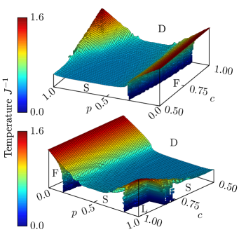
Figure 1: (Color online) Calculated global phase diagram of the $d=3$ chiral Potts spin glass, in temperature $J^{-1}$, chirality concentration $p$, and chirality-breaking concentration $c$. Note that the upper and lower figures are rotated with respect to each other. The ferromagnetically ordered phase (F), the chiral spin-glass phase (S), the left-chirally ordered phase (L), and the disordered phase (D) are marked. The global phase diagram is mirror-symmetric with respect to the chirality-breaking concentration $c=0.5$, so that only $1\leq c\leq 0.5$ is shown. In the (not shown) mirror-symmetric $0.5\leq c\leq 0$ portion of the global phase diagram, the right-chirally ordered phase (R) occurs in the place of the left-chirally ordered phase (L) seen in this figure. Different cross-sections of this global phase diagram are shown in Figs. 2 and 3.

I Introduction

The chiral Potts model was originally introduced Ostlund ; Kardar ; Huse ; Huse2 ; Caflisch to model the full phase diagram of krypton monolayers, including the epitaxial and incommensurate ordered phases. In addition to being useful in the analysis of surface layers, the chiral Potts model has become an important model of phase transitions and critical phenomena. We have studied the chiral spin-glass Potts system with $q=3$ states in $d=2$ and 3 spatial dimensions by renormalization-group theory and calculated the global phase diagrams (Fig. 1) in temperature, chirality concentration $p$, and chirality-breaking concentration $c$, also quantitatively determining phase chaos and phase-boundary chaos. In $d=3$, the system has ferromagnetic, left-chiral, right-chiral, chiral spin-glass, and disordered phases. The phase boundaries to the ferromagnetic, left- and right-chiral phases show, differently, an unusual, fibrous patchwork (microreentrances) of all four (ferromagnetic, left-chiral, right-chiral, chiral spin-glass) ordered phases, especially in the multicritical region. The chaotic behavior of the interactions, under scale change, is determined in the chiral spin-glass phase and on the boundary between the chiral spin-glass and disordered phases, showing Lyapunov exponents in magnitudes reversed from the usual ferromagnetic-antiferromagnetic spin-glass systems. At low temperatures, the boundaries of the left- and right-chiral phases become thresholded in $p$ and $c$. In the $d=2$, the chiral spin-glass Potts system does not have a spin-glass phase, consistently with the lower-critical dimension of ferromagnetic-antiferromagnetic spin glasses. The left- and right-chirally ordered phases show reentrance in chirality concentration $p$.

II The Chiral Potts Spin-Glass System

The chiral Potts model is defined by the Hamiltonian

$$\centering-\beta{\cal H}=\sum_{\left<ij\right>}[J_{0}\delta(s_{i},s_{j})+J_{\pm}\delta(s_{i},s_{j}\pm 1)],\@add@centering$$ (1)

where $\beta=1/k_{B}T$, at site $i$ the spin $s_{i}=1,2,,...,q$ can be in $q$ different states with implicit periodic labeling, e.g. $s_{i}=q+n$ implying $s_{i}=n$, the delta function $\delta(s_{i},s_{j})=1(0)$ for $s_{i}=s_{j}(s_{i}\neq s_{j})$, and $\langle ij\rangle$ denotes summation over all nearest-neighbor pairs of sites. The upper and lower subscripts of $J_{\pm}>0$ give left-handed and right-handed chirality (corresponding to heavy and superheavy domain walls in the krypton-on-graphite incommensurate ordering Kardar ; Caflisch ), whereas $J_{\pm}=0$ gives the non-chiral Potts model (relevant to the krypton-on-graphite epitaxial ordering BerkerPLG ).

In the chiral Potts spin-glass model studied here, the chirality of each nearest-neighbor interaction is randomly either left-handed, or right-handed, or zero. This randomness is frozen (quenched) into the system and the overall fraction of left-, right-, and non-chirality is controlled by the quenched densities $p$ and $c$ as described below. Thus, the Hamiltonian of the chiral Potts spin-glass model is

$$-\beta{\cal H}=\sum_{\left<ij\right>}J\,[(1-\eta_{ij})\delta(s_{i},s_{j})\\ +\eta_{ij}\,[\phi_{ij}\delta(s_{i},s_{j}+1)+(1-\phi_{ij})\delta(s_{i},s_{j}-1)],$$ (2)

where, for each pair of nearest-neighbor sites $<ij>,$ $\eta_{ij}=0$ (non-chiral) or 1 (chiral). In the latter case, $\phi_{ij}=1$ (left-handed) or 0 (right-handed). Thus, non-chiral, left-chiral, and right-chiral nearest-neighbor interactions are frozen randomly distributed in the entire system. For the entire system, the overall concentration of chiral interactions is given by $p$, with $0\leq p\leq 1$. Among the chiral interactions, the overall concentrations of left- and right-chiral interactions are respectively given by $c$ and $1-c$, with $0\leq c\leq 1$. Thus, the model is chiral for $p>0$ and chiral-symmetric $c=0.5$, chiral-symmetry broken for $c\neq 0.5$. The global phase diagram is given in terms of temperature $J^{-1}$, chirality concentration $p$, and chirality-breaking concentration $c$.(Figs. 1-3)

Under the renormalization-group transformations described below, the Hamiltonian given in Eq.(2) maps onto the more general form

$$-\beta{\cal H}=\sum_{\left<ij\right>}\,[J_{0}(ij)\delta(s_{i},s_{j})+J_{+}(ij)\delta(s_{i},s_{j}+1)\\ +J_{-}(ij)\delta(s_{i},s_{j}-1)],$$ (3)

where for each pair of nearest-neighbor sites $<ij>$, the largest of the interaction constants $(J_{0},J_{+},J_{-})$ is set to zero, by subtracting a constant G from each of $(J_{0},J_{+},J_{-})$, with no effect to the physics.

III Renormalization-Group Transformation: Migdal-Kadanoff Approximation / Exact Hierarchical Lattice Solution

We solve the chiral Potts spin-glass model with $q=3$ states by renormalization-group theory, in $d=3$ spatial dimension and with the length rescaling factor $b=2$. Our solution is, simultaneously, the Migdal-Kadanoff approximation Migdal ; Kadanoff for the cubic lattices and exact BerkerOstlund ; Kaufman1 ; Kaufman2 ; McKay ; Hinczewski1 for the $d=3$ hierarchical lattice based on the leftmost graph of Fig. 4. Exact calculations on hierarchical lattices BerkerOstlund ; Kaufman1 ; Kaufman2 ; McKay ; Hinczewski1 are also currently widely used on a variety of statistical mechanics problems Kaufman ; Kotorowicz ; Barre ; Monthus ; Zhang ; Shrock ; Xu ; Hwang2013 ; Herrmann1 ; Herrmann2 ; Garel ; Hartmann ; Fortin ; Wu ; Timonin ; Derrida ; Thorpe ; Efrat ; Monthus2 ; Hasegawa ; Lyra ; Singh ; Xu2014 ; Hirose1 ; Silva ; Hotta ; Boettcher1 ; Boettcher2 ; Hirose2 ; Boettcher3 ; Nandy . This approximation for the cubic lattice is an uncontrolled approximation, as in fact are all renormalization-group theory calculations in $d=3$ and all mean-field theory calculations. However, as noted before Yunus , the local summation in position-space technique used here has been qualitatively, near-quantitatively, and predictively successful in a large variety of problems, such as arbitrary spin-$s$ Ising models BerkerSpinS , global Blume-Emery-Griffiths model BerkerWortis , first- and second-order Potts transitions NienhuisPotts ; AndelmanBerker , antiferromagnetic Potts critical phases BerkerKadanoff1 ; BerkerKadanoff2 , ordering BerkerPLG and superfluidity BerkerNelson on surfaces, multiply reentrant liquid crystal phases Indekeu ; Garland , chaotic spin glasses McKayChaos , random-field Machta ; FalicovRField and random-temperature HuiBerker ; HuiBerkerE magnets including the remarkably small $d=3$ magnetization critical exponent $\beta$ of the random-field Ising model, and high-temperature superconductors HincewskiSuperc . Thus, this renormalization-group approximation continues to be widely used Gingras1 ; Migliorini ; Gingras2 ; Hinczewski ; Heisenberg ; Guven ; Ohzeki ; Ozcelik ; Gulpinar ; Kaplan ; Ilker1 ; Ilker2 ; Ilker3 ; Demirtas .

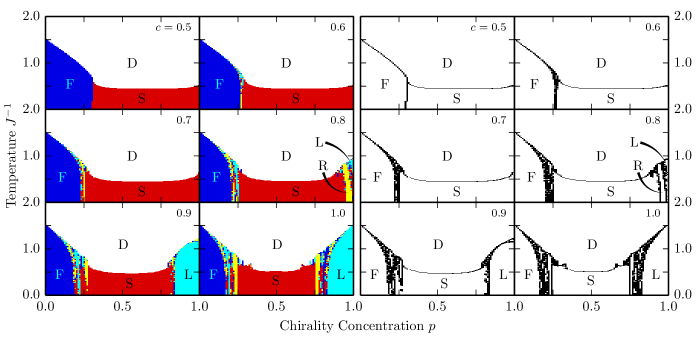
Figure 2: (Color online) Cross-sections, in temperature $J^{-1}$ and chirality concentration $p$, of the global phase diagram shown in Fig. 1. The chirality-breaking concentration $c$ is given on each cross-section. The ferromagnetically ordered phase (F), the chiral spin-glass phase (S), the left- and right-chirally ordered phases (L and R), and the disordered phase (D) are marked. Note that, as soon as the chiral symmetry of the model is broken by $c\neq 0.5$, a narrow fibrous patchwork (microreentrances) of all four (ferromagnetic, left-chiral, right-chiral, chiral spin-glass) ordered phases intervenes at boundaries of the ferromagnetically ordered phase F. This intervening region is more pronounced close to the multicritical region where the ferromagnetic, spin-glass, and disordered phases meet. The interlacing phase transitions inside this region are more clearly seen in the right-hand side panels of the figure, where only the phase boundaries are drawn in black. This intervening region gains importance as $c$ moves away from 0.5. But it is only at higher values of the chirality-breaking concentration $c$, such as $c=0.8$ on the figure, that the chirally ordered phase appears as a compact region at $c,p\lesssim 1$. In this case, again all four (ferromagnetic, left-chiral, right-chiral, chiral spin-glass) ordered phases intervene in a narrow fibrous patchwork at the boundaries of the chirally ordered phase L and R, the latter mirror-symmetric and not shown here. For $c=1$, for which all interactions of the system are, with respective concentrations $1-p$ and $p$, either ferromagnetic, or left-chiral, the phase diagram becomes symmetric with respect to $p=0.5$ as in standard ferromagnetic-antiferromagnetic spin-glass systems, except that the chirally ordered phases dominate the fibrous patchwork on both sides of the phase diagram.

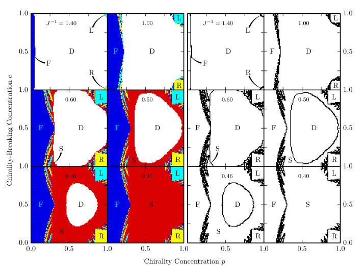
Figure 3: (Color online) Cross-sections, in chirality concentration $p$ and chirality-breaking concentration $c$, of the global phase diagram shown in Fig. 1. The temperature $J^{-1}$ is given on each cross-section. The ferromagnetically ordered phase (F), the chiral spin-glass phase (S), the left-chirally ordered phase (L), the right-chirally ordered phase (R), and the disordered phase (D) are marked. Note the narrow fibrous patches (microreentrances) of all four (ferromagnetic, left-chiral, right-chiral, chiral spin-glass) ordered phases intervening at the boundaries of the ferromagnetically ordered phase F and at the boundaries of the chirally ordered phases L and R. It is seen here that, within these regions, the chirally ordered phases L and R form elongated lamellar patterns. These intervening phase transitions are more clearly seen in the right-hand side panels of the figure, where only the phase boundaries are drawn in black. Also note the temperature-independent square shape, at low temperatures, of the phase boundary of the chirally ordered phases, creating thresholds of $p=0.84$ and $c=0.84$ or 0.16 into L or R, respectively. This is also visible in the three-dimensional Fig. 1

Figure 4: Renormalization-group transformation consisting of decimation followed by bond moving. The resulting recursion relations are approximate for the cubic lattice. The corresponding hierarchical lattice is obtained by the repeated self-imbedding of the leftmost graph. The recursion relations are exact for this $d=3$ hierarchical lattice. For the $d=2$, the number of parallel strands is 2 instead of 4 shown here.

The local renormalization-group transformation is achieved by a sequence, shown in Fig. 4, of decimations

$$\begin{split}e^{\widetilde{J}_{0}(13)-\widetilde{G}}=x_{0}(12)x_{0}(23)&+x_{+}(12)x_{-}(23)\\ &+x_{-}(12)x_{+}(23),\\ e^{\widetilde{J}_{+}(13)-\widetilde{G}}=x_{0}(12)x_{+}(23)&+x_{+}(12)x_{0}(23)\\ &+x_{-}(12)x_{-}(23),\\ e^{\widetilde{J}_{-}(13)-\widetilde{G}}=x_{0}(12)x_{-}(23)&+x_{-}(12)x_{0}(23)\\ &+x_{+}(12)x_{+}(23),\\ \end{split}$$ (4)

where $x_{0}(12)\equiv e^{J_{0}(12)}$, etc., and $\widetilde{G}$ is the subtractive constant mentioned in the previous section, and bond movings

$$\begin{split}J_{0}^{\prime}(13)=&\widetilde{J}_{0}^{(1)}(13)+\widetilde{J}_{0}^{(2)}(13)+\widetilde{J}_{0}^{(3)}(13)+\widetilde{J}_{0}^{(4)}(13),\\ J_{+}^{\prime}(13)=&\widetilde{J}_{+}^{(1)}(13)+\widetilde{J}_{+}^{(2)}(13)+\widetilde{J}_{+}^{(3)}(13)+\widetilde{J}_{+}^{(4)}(13),\\ J_{-}^{\prime}(13)=&\widetilde{J}_{-}^{(1)}(13)+\widetilde{J}_{-}^{(2)}(13)+\widetilde{J}_{-}^{(3)}(13)+\widetilde{J}_{-}^{(4)}(13),\end{split}$$ (5)

where primes mark the interactions of the renormalized system.

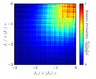
Figure 5: (Color online) The fixed probability distribution of the quenched random interactions $P_{0}(J_{+},J_{-})$ to which all of the points in the chiral spin-glass phase are attracted under renormalization-group transformations, namely the sink of the chiral spin-glass phase. The average interactions $<J_{\pm}>$ diverge to negative infinity as $<J_{\pm}>\sim b^{y_{R}n}$, where $n$ is the number of renormalization-group iterations and $y_{R}=0.32$ is the runaway exponent, while $J_{0}=0$ (See Sec. II). The other two distributions $P_{+}(J_{0},J_{-})$ and $P_{-}(J_{0},J_{+})$ have the same sink distribution. Thus, in the chiral spin-glass phase, chiral symmetry is broken by local order, but not globally.

The starting trimodal quenched probability distribution of the interactions, characterized by $p$ and $c$ as described above, is not conserved under rescaling. The renormalized quenched probability distribution of the interactions is obtained by the convolution Andelman

$$P^{\prime}(\textbf{J}(i^{\prime}j^{\prime}))=\\ \int{\left[\prod_{ij}^{i^{\prime}j^{\prime}}d\textbf{J}(ij)P(\textbf{J}(ij))\right]}\delta(\textbf{J}(i^{\prime}j^{\prime})-\textbf{R}(\left\{\textbf{J}(ij)\right\})),$$ (6)

where $\textbf{J}\equiv(J_{0}^{\prime},J_{+}^{\prime},J_{-}^{\prime})$ and $\textbf{R}(\left\{\textbf{J}(ij)\right\})$ represents the bond decimation and bond moving given in Eqs.(4) and (5). Similar previous studies, on other spin-glass systems, are in Refs. Gingras1 ; Migliorini ; Gingras2 ; Hinczewski ; Heisenberg ; Guven ; Ohzeki ; Ozcelik ; Gulpinar ; Kaplan ; Ilker1 ; Ilker2 ; Ilker3 ; Demirtas .

For numerical practicality, the bond moving of Eq. (5) is achieved by two sequential pairwise combination of interactions, each pairwise combination leading to an intermediate probability distribution resulting from a pairwise convolution as in Eq.(6). Furthermore, due to our convention of zeroing the largest interaction constant in each local triplet of interactions, the quenched probability distribution of three interactions $P(\textbf{J}(ij))$ is conveniently just composed of the three probability distributions of two interactions, $P_{0}(J_{+},J_{-}),P_{+}(J_{0},J_{-}),P_{-}(J_{+},J_{-})$, where $P_{0}(J_{+},J_{-})$ has the (largest) interaction $J_{0}=0,$ etc., which also considerably simplifies the numerical calculation. We effect this procedure numerically, by representing each probability distribution by histograms, as in previous studies Migliorini ; Hinczewski ; Heisenberg ; Guven ; Ozcelik ; Gulpinar ; Ilker2 ; Demirtas . The probability distributions of two interactions $P_{0}(J_{+},J_{-})$, $P_{+}(J_{0},J_{-})$, and $P_{-}(J_{+},J_{-})$ are represented via bivariate histograms with two-dimensional vectors $(J_{+},J_{-})$ for $P_{0}$, etc. The number of histograms grow rapidly with each renormalization-group transformation, so that for calculational purposes, the histograms are binned when the number of histograms outgrow $40,000$ bins. In the calculation of chiral spin-glass phase-sink fixed distribution of Fig. 5, the histograms are binned after $10^{8}$ histograms.

The different thermodynamic phases of the model are identified by the different asymptotic renormalization-group flows of the quenched probability distribution. For all renormalization-group flows, originating inside the phases and on the phase boundaries, Eq.(6) is iterated until asymptotic behavior is reached. Thus, we are able to calculate the global phase diagram of the chiral Potts spin-glass model.

IV Chiral Potts Spin Glass: Calculated Global Phase Diagram

The calculated global phase diagram of the $d=3$ chiral Potts spin-glass system, in temperature $J^{-1}$, chirality concentration $p$, and chirality-breaking concentration $c$, is given in Fig. 1. The ferromagnetically ordered (F) phase occurs at low temperature and low chirality $p$. The chiral spin-glass ordered (S) phase occurs at intermediate chirality $p$ for all $c$ and at high chirality $p$ for intermediate $c$. The left- and right-chirally ordered phases L and R occur at high chirality $p$ and values of chirality-breaking $c$ away from 0.5. The disordered phase (D) occurs at high temperature. The global phase diagram is mirror-symmetric with respect to the chirality-breaking concentration $c=0.5$, so that only $1\leq c\leq 0.5$ is shown in Fig. 1. In the (not shown) mirror-symmetric $0.5\leq c\leq 0$ portion of the global phase diagram, the right-chirally ordered phase (R) occurs in the place of the left-chirally ordered phase (L) seen in Fig. 1. Different cross-sections of the global phase diagram are shown in Figs. 2 and 3.

Under renormalization-group transformations, all points in the spin-glass phase are attracted to a fixed probability distribution of the quenched random interactions $P(J_{0},J_{+},J_{-})$, namely to the sink of the chiral spin-glass phase. As explained in Sec. III, $P(J_{0},J_{+},J_{-})$ is composed of three distributions, $P_{0}(J_{+},J_{-})$, $P_{+}(J_{0},J_{-})$, and $P_{-}(J_{0},J_{+})$. Of these, $P_{0}(J_{+},J_{-})$ gives the quenched probability distribution of nearest-neighbor interactions in which the ferromagnetic interaction $J_{0}$ is dominant. Similarly, $P_{+}(J_{0},J_{-})$ and $P_{-}(J_{0},J_{+})$ give the quenched probability distributions of nearest-neighbor interactions in which, respectively, the left-chiral interaction $J_{+}$ and the right-chiral interaction $J_{-}$ are dominant. (As explained in Sec. II, by subtraction of an overall constant, the dominant interaction is set to zero and the other two, subdominant interactions are therefore negative, with no loss of generality.) The sink fixed distribution for $P_{0}(J_{+},J_{-})$ is given in Fig. 5, where the average interactions $<J_{\pm}>$ diverge to negative infinity as $b^{y_{R}n}$, where $n$ is the number of renormalization-group iterations and $y_{R}=0.32$ is the runaway exponent, while conserving the shape of the distribution shown in Fig. 5. The other two distribution $P_{+}(J_{0},J_{-})$ and $P_{-}(J_{0},J_{+})$ have the same sink distribution. Thus, in the chiral spin-glass phase, chiral symmetry is broken by local order, but not globally.

In spin-glass phases, at a specific location in the lattice, the consecutive interactions, encountered under consecutive renormalization-group transformations, behave chaotically McKayChaos ; McKayChaos2 ; BerkerMcKay . This chaotic behavior was found McKayChaos ; McKayChaos2 ; BerkerMcKay and subsequently well established Bray ; Hartford ; Nifle1 ; Nifle2 ; Banavar ; Frzakala1 ; Frzakala2 ; Sasaki ; Lukic ; Ledoussal ; Rizzo ; Katzgraber ; Yoshino ; Pixley ; Aspelmeier1 ; Aspelmeier2 ; Mora ; Aral ; Chen ; Jorg ; Lima ; Katzgraber2 ; MMayor ; ZZhu ; Katzgraber3 ; Fernandez ; Ilker1 ; Ilker2 in spin-glass systems with competing ferromagnetic and antiferromagnetic interactions. We find here that the chaotic rescaling behavior also occurs in our current spin-glass system with competing left- and right-chiral interactions, as shown in Fig. 6. In fact, the chaotic rescaling behavior occurs not only within the spin-glass phase, but also, quantitatively distinctly, at the phase boundary between the spin-glass and disordered phases Ilker1 . This chaotic behavior at the phase boundary is also seen in the chiral system here and also shown in Fig. 6. It has been shown that chaos in the interaction as a function of rescaling implies chaos in the spin-spin correlation function as a function of distance Aral . Chaos in the spin-glass phase and at its phase boundary are identified and distinguished by different Lyapunov exponents Aral ; Ilker1 ; Ilker2 . We have calculated the Lyapunov exponent Collet ; Hilborn

$$\lambda=\lim_{n\rightarrow\infty}\frac{1}{n}\sum_{k=0}^{n-1}\ln\Big{|}\frac{dx_{k+1}}{dx_{k}}\Big{|}$$ (7)

where $x_{k}=J(ij)/<J>$ at step $k$ of the renormalization-group trajectory. The sum in Eq.(7) is to be taken within the asymptotic chaotic band, which is renormalization-group stable or unstable for the phase or its boundary, respectively. Thus, we throw out the first 100 renormalization-group iterations to eliminate the transient points outside of, but leading to the chaotic band. Subsequently, typically using 1,000 renormalization-group iterations in the sum in Eq.(7) assures the convergence of the Lyapunov exponent value. Thus, the Lyapunov exponents that we obtain are numerically exact, to the number of digits given. We have calculated the Lyapunov exponents $\lambda=1.77$ and 1.94 respectively for the chiral spin-glass phase and for the boundary between the chiral spin-glass and disordered phases. At the chiral spin-glass phase-sink fixed distribution, the average interaction diverges to negative infinity as $<J>\sim b^{ny_{R}}$, where $n$ is the number of renormalization-group iterations and $y_{R}=0.32$ is the runaway exponent. At the fixed distribution of the phase boundary between the chiral spin-glass and disordered phases, the average interaction remains fixed at $<J>=-2.53$. Interestingly, chaos is stronger at the boundary (larger Lyapunov exponent) than inside the chiral spin-glass phase. The opposite is seen in the usually studied $\pm J$ ferromagnetic-antiferromagnetic spin glass Ilker1 .

Figure 6: Chaotic renormalization-group trajectory: The three interactions at a given location, under consecutive renormalization-group transformations, are shown. Bottom panel: Inside the chiral spin-glass phase. The corresponding Lyapunov exponent is $\lambda=1.77$ and the average interaction diverges as $<J>\sim b^{y_{R}n}$, where $n$ is the number of renormalization-group iterations and $y_{R}=0.32$ is the runaway exponent. Top panel: At the phase boundary between the chiral spin-glass and disordered phases. The corresponding Lyapunov exponent is $\lambda=1.94$ and the average non-zero interaction is fixed at $<J>=-2.53$. The relative value of the Lyapunov exponents is unusual for spin-glass systems.

By contrast, in each of the ferromagnetic (F), left-chiral (L), and right-chiral (R) ordered phases, under consecutive renormalization-group transformations, the quenched probability distribution of the interactions sharpens to a delta function around a single value receding to negative infinity, for the respective pairs of interactions, namely ($J_{+},J_{-}),(J_{0},J_{+})$, and $(J_{0},J_{-})$. There is no asymptotic chaotic behavior under renormalization-group in these phases F, L, and R.

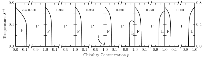
Figure 7: Representative cross-sections of the $d=2$ chiral Potts spin-glass system, in temperature $J^{-1}$ and chirality concentration $p$. The chirality-breaking concentration $c$ is given on each cross-section. The ferromagnetically ordered phase (F), the left-chirally ordered phase (L), and the disordered phase (D) are marked. No chiral spin-glass phase occurs in $d=2$ and no fibrous patchwork is seen at the phase boundaries. The chirally ordered phase appears for very high chirality-breaking concentration $c$ (seen here for $c=0.934$, but not seen for $c=0.930$) and shows reentrance in chirality concentration $p$. This reentrance disappears as $c=1$ is approached. For $c=1$, for which all interactions of the system are, with respective concentrations $1-p$ and $p$, either ferromagnetic, or left-chiral, the phase diagram becomes symmetric with respect to $p=0.5$ as in standard ferromagnetic-antiferromagnetic spin-glass systems.

Cross-sections of the global phase diagram, in temperature $J^{-1}$ and chirality concentration $p$, are given in Fig. 2. The chirality-breaking concentration $c$ is indicated for each cross-section. Note that, as soon as the chiral symmetry of the model is broken by $c\neq 0.5$, a narrow fibrous patchwork (microreentrances) of all four (ferromagnetic, left-chiral, right-chiral, chiral spin-glass) ordered phases intervenes at the boundaries between the ferromagnetically ordered phase F and the spin-glass phase S or the disordered phase D. This intervening region is more pronounced close to the multicritical region where the ferromagnetic, spin-glass, and disordered phases meet. The interlacing phase transitions inside this region are more clearly seen in the right-hand side panels of Fig. 2, where only the phase boundaries are drawn in black. This intervening region gains importance as $c$ moves away from 0.5. But it is only at higher values of the chirality-breaking concentration $c$, such as $c=0.8$ on the figure, that the chirally ordered phase appears as a compact region at $c,p\lesssim 1$. In this case, again all four (ferromagnetic, left-chiral, right-chiral, chiral spin-glass) ordered phases intervene in a narrow fibrous patchwork at the boundaries of the chirally ordered phases L and R, the latter mirror symmetric and not shown here. For $c=1$, for which all interactions of the system are, with respective concentrations $1-p$ and $p$, either ferromagnetic, or left-chiral, the phase diagram becomes symmetric with respect to $p=0.5$ as in standard ferromagnetic-antiferromagnetic spin-glass systems NishimoriBook , except that the chirally ordered phases dominate the fibrous patchwork on both sides of the phase diagram.

Cross-sections, in chirality concentration $p$ and chirality-breaking concentration $c$, of the global phase diagram are given in Fig. 3. The temperature $J^{-1}$ is given on each cross-section. Note the narrow fibrous patches of all four (ferromagnetic, left-chiral, right-chiral, chiral spin-glass) phases intervening at the boundaries of the ferromagnetically ordered phase F and at the boundaries of the chirally ordered phases L and R. It is seen here that, within these regions, the chirally ordered phases L and R form elongated lamellar patterns. The interlacing phase transitions inside this region are more clearly seen in the right-hand side panels of the figure, where only the phase boundaries are drawn in black. It is again seen that the symmetry around $p=0.5$ at the upper horizontal frame $(c=1)$ of each panel is broken inside the panel $(c<1)$. Also note the temperature-independent square shape, at low temperatures, of the phase boundary of the chirally ordered phases L and R, creating the threshold value of $p=0.84$ and $c=0.84$ or 0.16 into L or R, respectively. This is also visible in the three-dimensional Fig. 1.

V Chiral Reentrance in $d=2$

The global phase diagram of the $d=2$ chiral Potts spin-glass system is given in Fig. 7. Representative cross-sections in temperature $J^{-1}$ and chirality concentration $p$ are shown. The chirality-breaking concentration $c$ is given on each cross-section. The ferromagnetically ordered phase (F), the left-chirally ordered phase (L), and the disordered phase (D) are marked. No chiral spin-glass phase occurs in $d=2$ and no fibrous patchwork is seen at the phase boundaries. The chirally ordered phase appears for very high chirality-breaking concentration $c$ (seen here for $c=0.934$, but not seen for $c=0.930$) and shows reentrance Cladis ; Hardouin ; Indekeu ; Garland ; Netz ; Kumari ; Caflisch in chirality concentration $p$. This reentrance disappears as $c=1$ is approached. For $c=1$, for which all interactions of the system are, with respective concentrations $1-p$ and $p$, either ferromagnetic, or left-chiral, the phase diagram becomes symmetric with respect to $p=0.5$ as in standard ferromagnetic-antiferromagnetic spin-glass systems Ilker2 .

The absence of the chiral spin-glass phase in $d=2$ is consistent with standard ferromagnetic-antiferromagnetic Ising spin-glass systems, where the lower-critical dimension for the spin-glass phase is found around 2.5 Parisi ; Boettcher ; Amoruso ; Bouchaud ; Demirtas . Below this dimension, no spin-glass phase appears (unless some nano-restructuring is done to the system Ilker2 ).

VI Conclusion

We have thus obtained the global phase diagram of the chiral spin-glass Potts system with $q=3$ states in $d=3$ and 2 spatial dimensions by renormalization-group theory that is approximate for the cubic lattice and exact for the hierarchical lattice. Unusual features have been revealed in $d=3$. The phase boundaries to the ferromagnetic, left- and right-chiral phases show, differently, an unusual, fibrous patchwork (microreentrances) of all four (ferromagnetic, left-chiral, right-chiral, chiral spin-glass) ordered phases, especially in the multicritical region. In $d=3$, there is a chiral spin-glass phase. Quite unusually, the phase boundary between the chiral spin-glass and disordered phases is more chaotic than the chiral spin-glass phase itself, as judged by the magnitudes of the respective Lyapunov exponents. At low temperatures, the boundaries of the left- and right-chiral phases become temperature-independent and thresholded in chirality concentration $p$ and chirality-breaking concentration $c$. In the $d=2$, the chiral spin-glass system does not have a spin-glass phase, consistently with the lower-critical dimension of ferromagnetic-antiferromagnetic spin glasses. The left- and right-chirally ordered phases show reentrance in chirality concentration $p$.

- (1) S. Ostlund, Phys. Rev. 24, 398 (1981).
- (2) M. Kardar and A. N. Berker, Phys. Rev. Lett. 48, 1552 (1982).
- (3) D. A. Huse and M. E. Fisher, Phys. Rev. Lett. 49, 793 (1982).
- (4) D. A. Huse and M. E. Fisher, Phys. Rev. 29, 239 (1984).
- (5) R. G. Caflisch, A. N. Berker, and M. Kardar, Phys. Rev. B 31, 4527 (1985).
- (6) A. N. Berker, S. Ostlund, and F. A. Putnam, Phys. Rev. B 9, 3650 (1978).
- (7) A. A. Migdal, Zh. Eksp. Teor. Fiz. 69, 1457 (1975) [Sov. Phys. JETP 42, 743 (1976)].
- (8) L. P. Kadanoff, Ann. Phys. (N.Y.) 100, 359 (1976).
- (9) A. N. Berker and S. Ostlund, J. Phys. C 12, 4961 (1979).
- (10) R. B. Griffiths and M. Kaufman, Phys. Rev. B 26, 5022R (1982).
- (11) M. Kaufman and R. B. Griffiths, Phys. Rev. B 30, 244 (1984).
- (12) S. R. McKay and A. N. Berker, Phys. Rev. B 29, 1315 (1984).
- (13) M. Hinczewski and A. N. Berker, Phys. Rev. E 73, 066126 (2006).
- (14) M. Kaufman and H. T. Diep, Phys. Rev. E 84, 051106 (2011).
- (15) M. Kotorowicz and Y. Kozitsky, Cond. Matter Phys. 14, 13801 (2011).
- (16) J. Barre, J. Stat. Phys. 146, 359 (2012).
- (17) C. Monthus and T. Garel, J. Stat. Mech. - Theory and Experiment, P05002 (2012).
- (18) Z. Z. Zhang, Y. B. Sheng, Z. Y. Hu, and G. R. Chen, Chaos 22, 043129 (2012).
- (19) S.-C. Chang and R. Shrock, Phys. Lett. A 377, 671 (2013).
- (20) Y.-L. Xu, L.-S. Wang, and X.-M. Kong, Phys. Rev. A 87, 012312 (2013).
- (21) S. Hwang, D.-S. Lee, and B. Kahng, Phys. Rev. E 87, 022816 (2013).
- (22) R. F. S. Andrade and H. J. Herrmann, Phys. Rev. E 87, 042113 (2013).
- (23) R. F. S. Andrade and H. J. Herrmann, Phys. Rev. E 88, 042122 (2013).
- (24) C. Monthus and T. Garel, J. Stat. Phys. - Theory and Experiment, P06007 (2013).
- (25) O. Melchert and A. K. Hartmann, Eur. Phys. J. B 86, 323 (2013).
- (26) J.-Y. Fortin, J. Phys.-Condensed Matter 25, 296004 (2013).
- (27) Y. H. Wu, X. Li, Z. Z. Zhang, and Z. H. Rong, Chaos Solitons Fractals 56, 91 (2013).
- (28) P. N. Timonin, Low Temp. Phys. 40, 36 (2014).
- (29) B. Derrida and G. Giacomin, J. Stat. Phys. 154, 286 (2014).
- (30) M. F. Thorpe and R. B. Stinchcombe, Philos. Trans. Royal Soc. A - Math. Phys. Eng. Sciences 372, 20120038 (2014).
- (31) A. Efrat and M. Schwartz, Physica 414, 137 (2014).
- (32) C. Monthus and T. Garel, Phys. Rev. B 89, 184408 (2014).
- (33) T. Nogawa and T. Hasegawa, Phys. Rev. E 89, 042803 (2014).
- (34) M. L. Lyra, F. A. B. F. de Moura, I. N. de Oliveira, and M. Serva, Phys. Rev. E 89, 052133 (2014).
- (35) V. Singh and S. Boettcher, Phys. Rev. E 90, 012117 (2014).
- (36) Y.-L. Xu, X. Zhang, Z.-Q. Liu, K. Xiang-Mu, and R. Ting-Qi, Eur. Phys. J. B 87, 132 (2014).
- (37) Y. Hirose, A. Oguchi, and Y. Fukumoto, J. Phys. Soc. Japan 83, 074716 (2014).
- (38) V. S. T. Silva, R. F. S. Andrade, and S. R. Salinas, Phys. Rev. E 90, 052112 (2014).
- (39) Y. Hotta, Phys. Rev. E 90, 052821 (2014).
- (40) S. Boettcher, S. Falkner, and R. Portugal, Phys. Rev. A 91 052330 (2015).
- (41) S. Boettcher and C. T. Brunson, Eur. Phys. Lett. 110, 26005 (2015).
- (42) Y. Hirose, A. Ogushi, and Y. Fukumoto, J. Phys. Soc. Japan 84, 104705 (2015).
- (43) S. Boettcher and L. Shanshan, J. Phys. A 48, 415001 (2015).
- (44) A. Nandy and A. Chakrabarti, Phys. Lett. 379, 43 (2015).
- (45) Ç. Yunus, B. Renklioğlu, M. Keskin, and A. N. Berker, Phys. Rev. E 93, 062113 (2016).
- (46) A. N. Berker, Phys. Rev. B 12, 2752 (1975).
- (47) A. N. Berker and M. Wortis, Phys. Rev. B 14, 4946 (1976).
- (48) B. Nienhuis, A. N. Berker, E. K. Riedel, and M. Schick, Phys. Rev. Let. 43, 737 (1979).
- (49) D. Andelman and A. N. Berker, J. Phys. A 14, L91 (1981).
- (50) A. N. Berker and L. P. Kadanoff, J. Phys. A 13, L259 (1980).
- (51) A. N. Berker and L. P. Kadanoff, J. Phys. A 13, 3786 (1980).
- (52) A. N. Berker and D. R. Nelson, Phys. Rev. B 19, 2488 (19769).
- (53) J. O. Indekeu and A. N. Berker, Physica A 140, 368 (1986).
- (54) J. O. Indekeu, A. N. Berker, C. Chiang, and C. W. Garland, Phys. Rev. A 35, 1371 (1987).
- (55) S. R. McKay, A. N. Berker, and S. Kirkpatrick, Phys. Rev. Lett. 48, 767 (1982).
- (56) M. S. Cao and J. Machta, Phys. Rev. B 48, 3177 (1993).
- (57) A. Falicov, A. N. Berker, and S. R. McKay, Phys. Rev. B 51, 8266 (1995).
- (58) K. Hui and A. N. Berker, Phys. Rev. Lett. 62, 2507 (1989).
- (59) K. Hui and A. N. Berker, Phys. Rev. Lett. 63, 2433 (1989).
- (60) M. Hinczewski and A. N. Berker, Phys. Rev. B 78, 064507 (2008).
- (61) M. J. P. Gingras and E. S. Sørensen, Phys. Rev. B. 46, 3441 (1992).
- (62) G. Migliorini and A. N. Berker, Phys. Rev. B. 57, 426 (1998).
- (63) M. J. P. Gingras and E. S. Sørensen, Phys. Rev. B. 57, 10264 (1998).
- (64) M. Hinczewski and A.N. Berker, Phys. Rev. B 72, 144402 (2005).
- (65) C. N. Kaplan and A. N. Berker, Phys. Rev. Lett. 100, 027204 (2008).
- (66) C. Güven, A. N. Berker, M. Hinczewski, and H. Nishimori, Phys. Rev. E 77, 061110 (2008).
- (67) M. Ohzeki, H. Nishimori, and A. N. Berker, Phys. Rev. E 77, 061116 (2008).
- (68) V. O. Özçelik and A. N. Berker, Phys. Rev. E 78, 031104 (2008).
- (69) G. Gülpınar and A. N. Berker, Phys. Rev. E 79, 021110 (2009).
- (70) C.N. Kaplan, M. Hinczewski, and A.N. Berker, Phys. Rev. E 79, 061120 (2009).
- (71) E. Ilker and A. N. Berker, Phys. Rev. E 87, 032124 (2013).
- (72) E. Ilker and A. N. Berker, Phys. Rev. E 89, 042139 (2014).
- (73) E. Ilker and A. N. Berker, Phys. Rev. E 90, 062112 (2014).
- (74) M. Demirtaş, A. Tuncer, and A. N. Berker, Phys. Rev. E 92, 022136 (2015).
- (75) D. Andelman and A. N. Berker, Phys. Rev. B 29, 2630 (1984).
- (76) S. R. McKay, A. N. Berker, and S. Kirkpatrick, J. Appl. Phys. 53, 7974 (1982).
- (77) A. N. Berker and S. R. McKay, J. Stat. Phys. 36, 787 (1984).
- (78) A. J. Bray and M. A. Moore, Phys. Rev. Lett. 58, 57 (1987).
- (79) E. J. Hartford and S. R. McKay, J. Appl. Phys. 70, 6068 (1991).
- (80) M. Nifle and H. J. Hilhorst, Phys. Rev. Lett. 68, 2992 (1992).
- (81) M. Nifle and H. J. Hilhorst, Physica A 194, 462 (1993).
- (82) M. Cieplak, M. S. Li, and J. R. Banavar, Phys. Rev. B 47, 5022 (1993).
- (83) F. Krzakala, Europhys. Lett. 66, 847 (2004).
- (84) F. Krzakala and J. P. Bouchaud, Europhys. Lett. 72, 472 (2005).
- (85) M. Sasaki, K. Hukushima, H. Yoshino, and H. Takayama, Phys. Rev. Lett. 95, 267203 (2005).
- (86) J. Lukic, E. Marinari, O. C. Martin, and S. Sabatini, J. Stat. Mech.: Theory Exp. L10001 (2006).
- (87) P. Le Doussal, Phys. Rev. Lett. 96, 235702 (2006).
- (88) T. Rizzo and H. Yoshino, Phys. Rev. B 73, 064416 (2006).
- (89) H. G. Katzgraber and F. Krzakala, Phys. Rev. Lett. 98, 017201 (2007).
- (90) H. Yoshino and T. Rizzo, Phys. Rev. B 77, 104429 (2008).
- (91) J. H. Pixley and A. P. Young, Phys Rev B 78, 014419 (2008).
- (92) T. Aspelmeier, Phys. Rev. Lett. 100, 117205 (2008).
- (93) T. Aspelmeier, J. Phys. A 41, 205005 (2008).
- (94) T. Mora and L. Zdeborova, J. Stat. Phys. 131, 1121 (2008).
- (95) N. Aral and A. N. Berker, Phys. Rev. B 79, 014434 (2009).
- (96) Q. H. Chen, Phys. Rev. B 80, 144420 (2009).
- (97) T. Jörg and F. Krzakala, J. Stat. Mech.: Theory Exp. L01001 (2012).
- (98) W. de Lima, G. Camelo-Neto, and S. Coutinho, Phys. Lett. A 377, 2851 (2013).
- (99) W. Wang, J. Machta, and H. G. Katzgraber, Phys. Rev. B 92, 094410 (2015).
- (100) V. Martin-Mayor and I. Hen, Scientific Repts. 5, 15324 (2015)
- (101) Z. Zhu, A. J. Ochoa, S. Schnabel, F. Hamze, and H. G. Katzgraber, Phys. Rev. A 93, 012317 (2016).
- (102) W. Wang, J. Machta, and H. G. Katzgraber, Phys. Rev. B 93, 224414 (2016).
- (103) L. A. Fernandez, E. Marinari, V. Martin-Mayor, G. Parisi, and D. Yllanes, arXiv:1605.03025 [cond-mat.dis-nn] (2016).
- (104) P. Collet and J.-P. Eckmann, Iterated Maps on the Interval as Dynamical Systems (Birkhäuser, Boston, 1980).
- (105) R. C. Hilborn, Chaos and Nonlinear Dynamics, 2nd ed. (Oxford University Press, New York, 2003).
- (106) H. Nishimori, Statistical Physics of Spin Glasses and Information Processing (Oxford University Press, Oxford, 2001).
- (107) P. E. Cladis, Phys. Rev. Lett. 35, 48 (1975).
- (108) F. Hardouin, A. M. Levelut, M. F. Achard, and G. Sigaud, J. Chim. Phys. 80, 53 (1983).
- (109) R. R. Netz and A. N. Berker, Phys. Rev. Lett. 68, 333 (1992).
- (110) S. Kumari and S. Singh, Phase Transitions 88, 1225 (2015).
- (111) S. Franz, G. Parisi, and M.A. Virasoro, J. Physique I 4, 1657 (1994).
- (112) S. Boettcher, Phys. Rev. Lett. 95, 197205 (2005).
- (113) C. Amoruso, E. Marinari, O. C. Martin, and A. Pagnani, Phys. Rev. Lett. 91, 087201 (2003).
- (114) J.-P. Bouchaud, F. Krzakala, and O. C. Martin, Phys. Rev. B 68, 224404 (2003).