Sample-to-sample fluctuations of power spectrum of a random motion in a periodic Sinai model

Abstract

The Sinai model of a tracer diffusing in a quenched Brownian potential is a much studied problem exhibiting a logarithmically slow anomalous diffusion due to the growth of energy barriers with the system size. However, if the potential is random but periodic, the regime of anomalous diffusion crosses over to one of normal diffusion once a tracer has diffused over a few periods of the system. Here we consider a system in which the potential is given by a Brownian Bridge on a finite interval $(0,L)$ and then periodically repeated over the whole real line, and study the power spectrum $S(f)$ of the diffusive process $x(t)$ in such a potential. We show that for most of realizations of $x(t)$ in a given realization of the potential, the low-frequency behavior is $S(f)\sim{\cal A}/f^{2}$, i.e., the same as for standard Brownian motion, and the amplitude ${\cal A}$ is a disorder-dependent random variable with a finite support. Focusing on the statistical properties of this random variable, we determine the moments of ${\cal A}$ of arbitrary, negative or positive order $k$, and demonstrate that they exhibit a multi-fractal dependence on $k$, and a rather unusual dependence on the temperature and on the periodicity $L$, which are supported by atypical realizations of the periodic disorder. We finally show that the distribution of ${\cal A}$ has a log-normal left tail, and exhibits an essential singularity close to the right edge of the support, which is related to the Lifshitz singularity. Our findings are based both on analytic results and on extensive numerical simulations of the process $x(t)$.

The statistical classification of time dependent stochastic processes is often based on the study of their power spectrum

$$S(f)=\lim_{T\to\infty}\overline{\left|\int^{T}_{0}dt\;\,e^{ift}\;x(t)\right|^{2}}\,,$$ (1)

where the horizontal bar denotes ensemble averaging with respect to all possible realizations of $x(t)$. Many processes, which are common in nature and are often observed in engineering and technological sciences, are found to exhibit a low-frequency noise spectrum of the universal form man ; dutta

$$S(f)\sim\dfrac{{\cal A}}{f^{\alpha}}\,.$$ (2)

The amplitude ${\cal A}$ is independent of $f$, and the exponent $\alpha\in(1,2)$, with the extreme cases $\alpha=1$ and $\alpha=2$ corresponding to the $1/f$ (flicker) noise and Brownian noise (or noise of the extremes of Brownian noise gleb ), respectively. There exist a few physical cases for which the form in (2) with $\alpha<2$ extends over many decades in frequency, implying the existence of correlations over surprisingly long times. Relevant examples include electrical signals in vacuum tubes, semiconductor devices and metal films man ; dutta . More generally, the form in (2) is observed in sequences of earthquakes 5 and weather data wea , in evolution 7 , human cognition 8 , network traffic 9 and even in the temporal distribution of loudness in musical recordings press . Recent experiments have shown the occurrence of such universal spectra in processes taking place in a variety of nanoscale systems. Among them are transport in individual ionic channels 10 ; 11 and electrochemical signals in nanoscale electrodes 13 , bio-recognition processes 14 and intermittent quantum dots 15 . Many other examples, related theoretical concepts, emerging challenges and unresolved problems have been discussed in 15 ; enzo ; enzo1 ; mike ; 16 ; 17 .

An example of a transport process which exhibits the flicker $1/f$ noise (with logarithmic corrections) was pointed out more than 30 years ago in enzo ; enzo1 . This is a paradigmatic example for random motion in a quenched random environment, now known as Sinai diffusion sinai , which has been studied in many different contexts bou1 ; osh1 ; osh2 ; mon ; alb ; com ; sid . Sinai diffusion is defined as a Brownian motion advected by a quenched drift which is time independent and uncorrelated in space. It can thus be seen as an over-damped Langevin process subject to a quenched force which is uncorrelated in space, so that in one dimension it is derived from a Brownian potential $V(x)$. The mean-square displacement of the Sinai diffusion exhibits a remarkably slow logarithmically growth with time $t$,

$$\mathbb{E}\left(\overline{x^{2}(t)}\right)\sim\ln^{4}(t)\;,\,\,\,t\to\infty\,,$$ (3)

where $\mathbb{E}(\cdot)$ denotes averaging over realizations of the random potential. The result in (3) is supported by typical realizations of disorder,i.e., it holds for almost all samples with a given potential $V(x)$. Note that despite the slow logarithmic dispersion of the trajectories, the probability currents $J_{L}$ through finite samples of Sinai chains of length $L$ appear to be much larger than the Fickian currents in homogeneous systems osh1 ; osh2 ; mon ; alb ; for finite Sinai chains one has $\mathbb{E}(J_{L})\sim 1/\sqrt{L}$, while for homogeneous systems $J_{L}\sim 1/L$. Such an anomalous behavior of currents is supported by rare atypical realizations of $V(x)$ which however produce the dominant contributions to the average.

Figure 1: Potential $V(x)$ as a periodically extended Brownian Bridge with $V(x=0)=V(x=L)=0$.

In this paper we analyze the power spectrum of random motion in a random quenched potential looking at the problem from a different perspective - we will mainly focus on the amplitude ${\cal A}$ of the power spectrum, not on the value of the exponent $\alpha$ characterizing the power spectrum. In random environments, this amplitude is itself a random variable fluctuating from realization to realization of the random potential, this makes the power spectrum itself a random variable. Here we concentrate on a particular model - a periodic Sinai chain dean , in which the potential is a finite Brownian trajectory with constrained endpoint - the so-called Brownian Bridge, defined on the interval $(0,L)$ and then periodically extended in both directions to give an infinite one-dimensional system (see Fig.1). The origin of the slow logarithmic growth in the original Sinai model (with $L=\infty$) is due to the unlimited growth of the Brownian potential and the associated energy barriers, however in our periodic case $x(t)$ ultimately converges to a Brownian motion, on large time and length scales, so that the low frequency spectrum has a form in (2) with $\alpha=2$ but the amplitude ${\cal A}$ - a positive random variable with a finite support $(0,{\cal A}_{r})$ - fluctuates from sample to sample. We determine the moments of ${\cal A}$ and show that the probability distribution function $P({\cal A})$ has a rather non-trivial form characterized by a log-normal left tail (in the vicinity of $0$) and a singular right tail (in the vicinity of the right edge ${\cal A}_{r}$ of the support). In general, ${\cal A}$ is not self-averaging and its moments are supported by atypical realizations of disorder. These analytic predictions for the periodic Sinai model are confirmed by extensive numerical simulations. An analysis of the distribution of ${\cal A}$ for the original Sinai model with $L\equiv\infty$, where the spectrum is described by (2) with $\alpha=1$ enzo ; enzo1 will be presented elsewhere.

The precise definition of the model studied is as follows. Consider the Langevin dynamics of a tracer $x(t)$ in a time-independent potential $V\left(x\right)$:

$$\eta\dfrac{dx(t)}{dt}=-\dfrac{dV\left(x(t)\right)}{dx(t)}+\xi_{t}\,,$$ (4)

where $\eta$ is the friction coefficient, $\xi_{t}$ is a Gaussian white noise with zero mean and covariance

$$\overline{\xi_{t}\xi_{t^{\prime}}}=2\eta T\delta(t-t^{\prime})\,,$$ (5)

and $T$ is the temperature in units of the Boltzmann constant. The potential is periodic, such that $V\left(x+L\right)=V\left(x\right)$, with $L$ being the periodicity.

Furthermore, we assume that the potential $V(x)$ on the interval $x\in(0,L)$ is a stochastic, continuous Gaussian process, pinned at both ends so that $V(0)=V(L)=0$, having zero mean and covariance

$$\mathbb{E}\left(V(x)V(y)\right)={2D_{V}}\left[{\rm min}(x,y)-\frac{xy}{L}\right]\,,\,\,0\leq x,\,y\leq L\,,$$ (6)

where $D_{V}=V_{0}^{2}/(2l)$, $V_{0}$ being a characteristic extent of the potential on a small scale of size $l$. In other words, $V(x)$ on the interval $(0,L)$ is the so-called Brownian Bridge (BB in what follows) mor which has the representation

$$V(x)=W_{x}-\frac{x}{L}W_{L},$$ (7)

where $W_{x}$ is a standard Brownian motion started at $W_{0}=0$ with correlation function

$$\mathbb{E}\left(W_{x}W_{y}\right)=2D_{V}{\rm min}(x,y)\;.$$ (8)

The overall potential on the entire $x$-axis is then given by a periodically repeated realization of the BB (see Fig. 1). Without loss of generality we set $l=1$ in what follows, meaning that we measure $L$ in units of $l$. We will also skip insignificant numerical factors focusing only on the dependence on the pertinent parameters, such as $T$, $L$ and $V_{0}$.

Before we proceed, it is important to emphasize that the dynamics in Eq.(4) represents a combination of two paradigmatic situations: random motion in a periodic potential and the Sinai dynamics. Consequently, we expect that $x(t)$ will exhibit two distinct temporal behaviors. At sufficiently short times t, $t\ll t_{c}$, where $t_{c}$ is a crossover time, the periodicity will not matter and the evolution of $x(t)$ will proceed exactly in the same fashion as in the original Sinai model, (3). At longer times, $t\gg t_{c}$, the periodicity of the potential will ensure a transition to a standard diffusive behavior, so that $x(t)$ will converge to

$$x(t)\sim\sqrt{2D[V(x)]}\,B_{t}\,,$$ (9)

where $B_{t}$ is a Brownian trajectory with diffusion coefficient $1$ and $D[V(x)]$ is a sample-dependent diffusion coefficient (see, e.g., lif ; ar ; hang ; dav ):

$$D[V(x)]=D_{0}/\left(\int^{L}_{0}\dfrac{dx}{L}\int^{L}_{0}\dfrac{dy}{L}\exp\left(\dfrac{V(x)-V(y)}{T}\right)\right)$$ (10)

where $D_{0}=T/\eta$ is the bare diffusion coefficient in absence of disorder. Note that $D[V(x)]\leq D_{0}$ lif so that $D[V(x)]$ is a random variable with support on $(0,D_{0})$.

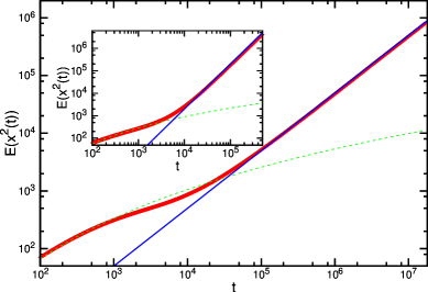
Figure 2: (color online) Main: $\mathbb{E}\left(\overline{x^{2}(t)}\right)$ in a periodic Sinai model (with a periodic BB), numerical data shown as points. Also shown by the dashed line is the fit $c_{1}\ln^{4}(t)$ for the short time Sinai regime along with the solid line late time fit $c_{2}t$. Inset: as in the main figure, but for an unconstrained periodic Sinai potential.

In the main plot of Fig. 2 we show the temporal evolution of $\mathbb{E}\left(\overline{x^{2}(t)}\right)$ in a periodic BB Sinai model, with $L=64$. The numerical evidence for the existence of the two temporal regimes described in (3) (at short times) and in (9) (at large times) is clear. We plot with points the numerical data averaged over 500000 realizations of the random quenched potential. The dashed line is $\ln^{4}(t)$ and agrees with the simulated data in the time region $(100,1000)$, while the continuous thin straight line is $t$ and fits perfectly the asymptotically large time region (say from $t_{\mbox{min}}=10^{5}$).

An intermediate very slow regime, where both the $\ln^{4}(t)$ and the $t$ dependence fail to fit the data, also appears clearly. Such a departure from the $\ln^{4}(t)$ law is not observed for a periodic unconstrained Sinai potential, that we show in the inset, again for $L=64$ (here the transition is from a Sinai to a ballistic regime, since for any finite $L$ the potential is biased yielding an constant, but random from sample to sample, force superimposed on a periodic potential). As a matter of fact, this is a surprising feature since one may intuitively expect that in the case of a BB potential the typical barrier which a particle has to overcome should be less, due to stronger correlations, than that for an unconstrained Brownian potential, so that for a BB the mean-square displacement $\mathbb{E}\left(\overline{x^{2}(t)}\right)$ should grow faster with time. This appears not to be the case and an apparent explanation is that for the BB potential the structure of a typical barrier which a particle has to bypass is different from the one for an unconstrained Brownian motion. This may be related to the recent observation gleb2 that the variance of a maximal positive displacement of a BB on some sub-interval $(0,L_{1})$ with $L_{1}<L$, may be greater than the variance of the maximal displacement on the entire interval $(0,L)$.

The inset helps us noticing that the transition from the Sinai regime at short times to the long time regime is not smeared in time but is sharp, and allows to consistently define a well-defined value of a transition time $t_{c}$, which we will discuss below. Accounting for the intermediate, sub-diffusive regime that appears in the case of the Sinai periodically repeated Brownian bridge, the same procedure allows to define a transition time also in this case. We may expect that for $t\gg t_{c}$, the typical behavior of $x(t)$ will be diffusive, so that the low-frequency ($f\ll 1/t_{c}$) behavior of the power spectrum (1) will have the form of (2) with $\alpha=2$

$$\dfrac{{\cal A}}{4D_{0}}=\dfrac{1}{\int^{L}_{0}\dfrac{dx}{L}\int^{L}_{0}\dfrac{dy}{L}\exp\left(\dfrac{V(x)-V(y)}{T}\right)}\,.$$ (11)

Taking into account that for a standard Brownian motion with the diffusion coefficient $D$ the amplitude in (2) is ${\cal A}=4D$, we expect ${\cal A}$ to have support $(0,4D_{0})$. In what follows we will focus on the statistical properties of ${\cal A}$.

We start by analyzing the typical behavior of ${\cal A}$ based on an estimate for the typical value of $\cal A$ that we call ${\cal A}_{typ}$:

$$\dfrac{{\cal A}_{typ}}{4D_{0}}\sim\exp\left(\mathbb{E}\left(\ln\left(\dfrac{{\cal A}}{4D_{0}}\right)\right)\right).$$ (12)

Furthermore,

$$\mathbb{E}\left(\ln\left(\dfrac{{\cal A}}{4D_{0}}\right)\right)=\mathbb{E}\left(\ln J_{L}^{+}\right)+\mathbb{E}\left(\ln J_{L}^{-}\right)+2\ln(L)\;,$$ (13)

where $J_{L}^{+}$ and $J_{L}^{-}$ are stationary currents through a finite, of length $L$ sample of a Sinai chain,

$$J_{L}^{+}=\dfrac{1}{\int^{L}_{0}dx\exp\left(\dfrac{V(x)}{T}\right)}\,,$$

$$J_{L}^{-}=\dfrac{1}{\int^{L}_{0}dy\exp\left(-\dfrac{V(y)}{T}\right)}\,.$$ (14)

Note that since $\mathbb{E}\left(V(x)\right)=0$, moments of arbitrary order obey $\mathbb{E}\left(\left(J_{L}^{+}\right)^{k}\right)\equiv\mathbb{E}\left(\left(J_{L}^{-}\right)^{k}\right)$ so that

$$\mathbb{E}\left(\ln J_{L}^{+}\right)\equiv\mathbb{E}\left(\ln J_{L}^{-}\right)$$ (15)

and thus

$$\mathbb{E}\left(\ln\left(\dfrac{{\cal A}}{4D_{0}}\right)\right)=2\mathbb{E}\left(\ln J_{L}^{+}\right)+2\ln(L).$$ (16)

The statistical properties of the currents in finite Sinai chains have been analyzed in osh1 ; osh2 ; mon ; alb for the case where $V(x)$ is an unconstrained Brownian or an unconstrained fractional Brownian motion. It was shown (see, e.g. alb for more details) that for sufficiently large values of $L$, the behavior of $J_{L}^{+}$ is dominated by the maximum of $V(x)$, $V_{max}\equiv{\rm max}_{0\leq x\leq L}V(x)$. Moreover, for any given realization of disorder $J_{L}^{+}$ can be bounded from below and from above by $A_{1}\exp(-V_{max}/T)$ and $A_{2}\exp(-V_{max}/T)$, where $A_{1}\leq A_{2}$ are $L$-independent constants. Consequently, the $L$-dependence (up to an insignificant numerical factor) is captured by the estimate $J_{L}^{+}\sim\exp(-V_{max}/T)$.

In principle, this argument can be readily generalized for the case at hand, when $V(x)$ is a BB, and we have merely to use the distribution $P_{BB}(V_{max})$ of a maximal positive displacement of a BB on an interval $(0,L)$, instead of the analogous distribution for an unconstrained Brownian motion used in alb . This distribution $P_{BB}(V_{max})$ is well-known from the classical papers kol ; sm ; fel , and is given by

$$P_{BB}(V_{max})=\dfrac{2V_{max}}{D_{V}L}\exp\left(-\dfrac{V_{max}^{2}}{D_{V}L}\right)\,,$$ (17)

where $D_{V}=V_{0}^{2}/(2l)$. Using (17), we find that, dropping numerical constants,

$$\mathbb{E}\left(\ln\left(\dfrac{{\cal A}}{4D_{0}}\right)\right)\sim-\dfrac{V_{0}}{T}L^{1/2}\,,$$ (18)

so that, for arbitrary values of $k$,

$$\left(\dfrac{{\cal A}_{typ}}{4D_{0}}\right)^{k}\sim\exp\left(-k\dfrac{V_{0}}{T}L^{1/2}\right)\,.$$ (19)

Therefore, we expect that, for most realizations of the random potential $V(x)$, the amplitude ${\cal A}$ of the power spectrum will decrease, as a stretched-exponential function $\exp(-L^{1/2})$ of the periodicity $L$, and will exhibit an Arrhenius dependence on the temperature $T$.

Next we consider the behavior of the moments $\mathbb{E}({\cal A}^{k})$ of the amplitude with arbitrary (positive or negative) values of $k$. When $V(x)$ is an unconstrained Brownian motion, a general analysis of the functional in (10) or (11) has been presented in dean . The disorder-average value (first moment) of this very functional, which also describes the ground-state energy in a one-dimensional localization problem, was determined in burl . It was shown in dean ; burl that the functional of the random potential in (10) or (11) can be bounded from below and from above by $B_{1}\exp(-R/T)$ and $B_{2}\exp(-R/T)$, where $B_{1}\leq B_{2}$ weakly depend on $L$ and

$$R\equiv{\rm max}_{0\leq x\leq L}V(x)-{\rm min}_{0\leq x\leq L}V(x)$$ (20)

is the range, or span, of the random potential $V(x)$. Physically $R$ corresponds to the largest energy barrier that will be encountered by the tracer. Expecting that $\mathbb{E}({\cal A}^{k})$ will show a stronger than a power-law dependence on $L$ (and we will show in what follows that it is the case) we may drop the constants $B_{1}$ and $B_{2}$ and write an estimate

$${\cal A}^{k}\sim\exp(-kR/T)\,,$$ (21)

which should capture the $L$, $k$ and $T$ dependence of the moments up to insignificant pre-exponential factors.

To extend this analysis over the case of a BB potential and in order to calculate the moments of ${\cal A}$ for the case under study, we need to know the distribution of the range of a BB. This distribution was first derived in feller , in which $R$ was referred to as an adjusted range of Brownian motion, and it is given in series form as

$$P_{BB}(R)=R\dfrac{d^{2}f(R)}{dR^{2}}+\sum_{n=2}^{\infty}\Bigg{[}2n(n-1)\Bigg{(}\dfrac{df((n-1)R)}{dR}-$$

$$-\dfrac{df(nR)}{dR}\Bigg{)}+(n-1)^{2}R\dfrac{d^{2}f((n-1)R)}{dR^{2}}+n^{2}R\dfrac{d^{2}f(nR)}{dR^{2}}\Bigg{]}\,,$$ (22)

where, in our notation, $f(R)=\exp(-R^{2}/D_{V}L)$. For our purposes a slightly different form of $P_{BB}(R)$ will also turn out to be useful. To this end, we exploit here the observation made in ken that the range of Brownian Bridge and the maximum of Brownian excursion - a Brownian Bridge constrained to stay positive - have the same distributions. The distribution of the maximum of a Brownian excursion has been extensively discussed in the literature and several forms of it have been derived (see for example yor ). Choosing a suitable one, we have, in our notation,

$$P_{BB}(R)=\sqrt{2}\pi^{5/2}(2D_{V}L)^{3/2}\times$$

$$\dfrac{d}{dR}\left(\dfrac{1}{R^{3}}\sum_{n=1}^{\infty}n^{2}\exp\left(-\dfrac{\pi^{2}n^{2}}{R^{2}}D_{V}L\right)\right)\,.$$ (23)

The two expressions (Sample-to-sample fluctuations of power spectrum of a random motion in a periodic Sinai model) and (Sample-to-sample fluctuations of power spectrum of a random motion in a periodic Sinai model) coincide.

Now we have all necessary ingredient to calculate the moments of ${\cal A}$. Consider first the moments of negative (not necessarily integer) order. Using the form of $P_{BB}(R)$ in (Sample-to-sample fluctuations of power spectrum of a random motion in a periodic Sinai model), and keeping only the leading exponential dependence on $R$, we average the estimate in (21) to obtain

$$\mathbb{E}\left(\left(\dfrac{4D_{0}}{{\cal A}}\right)^{k}\right)\sim\int^{\infty}_{0}dR\exp\left(\dfrac{k\,R}{T}-\dfrac{R^{2}}{D_{V}L}\right)$$ (24)

Evaluating this integral via steepest descent, we find that the maximum of the exponential is attained at $R\sim R^{*}=kD_{V}L/2T$, and thus

$$\mathbb{E}\left(\left(\dfrac{4D_{0}}{{\cal A}}\right)^{k}\right)\sim\exp\left(\dfrac{k^{2}\,V_{0}^{2}}{8T^{2}}L\right)\,.$$ (25)

Therefore, the negative moments grow faster than exponentially with $k$ and $V_{0}$, exhibit a super-Arrhenius dependence on the temperature and grow exponentially with the periodicity $L$.

The negative moments may also be computed directly by taking the average over the replicated 2$k$-fold integral to obtain

$$\mathbb{E}\left(\left(\dfrac{4D_{0}}{{\cal A}}\right)^{k}\right)=\int_{0}^{1}\ldots\int^{1}_{0}\prod_{a=1}^{k}du_{a}dw_{a}\times$$

$$\exp\Bigg{(}-\frac{D_{V}L}{2T^{2}}\Bigg{(}\sum_{a,b}|u_{a}-u_{b}|+|w_{a}-w_{b}|$$

$$-2|u_{a}-w_{b}|+2\left(\sum_{a}u_{a}-\sum_{a}w_{a}\right)^{2}\Bigg{)}\Bigg{)},$$ (26)

where we have rewritten the integration variables using $x_{a}=Lu_{a}$ and $y_{a}=Lw_{a}$ to obtain the above. The right hand side of (26) has the form of a partition function for $k+k$ interacting particles of two types $u$ and $w$ at inverse temperature $\beta=D_{V}L/2T^{2}$. In the limit of large $L$ the partition function is dominated by the ground state energy. The Hamiltonian is explicitly given by

$$H=\sum_{a,b}|u_{a}-u_{b}|+|w_{a}-w_{b}|-2|u_{a}-w_{b}|+2(\sum_{a}u_{a}-\sum_{a}w_{a})^{2}\;.$$ (27)

The particles of type $u$ and $w$ attract particles of the same type with a linear attractive potential, and they repel particles of the other type, again with a linear potential. However there is an additional interaction which harmonically binds the center of masses of the two particle types. Due to the attraction between the same particle type we expect that particles of the same type will condense at low temperature about the same point and hence we write $u_{a}=U$ and $w_{a}=W$ for all $a$. This gives the effective reduced low temperature Hamiltonian

$$H_{0}=2k^{2}(\Delta^{2}-\Delta)=2k^{2}(\Delta-\frac{1}{2})^{2}-\frac{k^{2}}{2}\;,$$ (28)

where $\Delta=|U-W|$. The value $\Delta=1/2$ minimizes the energy leading to

$$\mathbb{E}\left(\left(\dfrac{4D_{0}}{{\cal A}}\right)^{k}\right)\sim\exp(\frac{D_{V}k^{2}L}{4T^{2}})=\exp(\frac{k^{2}V_{0}^{2}L}{8T^{2}})\;,$$ (29)

in complete agreement with (25).

For positive moments of the amplitude, we use the form of $P_{BB}(R)$ in (Sample-to-sample fluctuations of power spectrum of a random motion in a periodic Sinai model). Keeping only the leading term in $L$, we find that the leading behavior of ${\cal A}^{k}$ in (21) is given by

$$\mathbb{E}\left(\left(\dfrac{{\cal A}}{4D_{0}}\right)^{k}\right)\sim\int^{\infty}_{0}dR\exp\left(-\dfrac{k\,R}{T}-\dfrac{\pi^{2}D_{V}L}{R^{2}}\right)\,.$$ (30)

Again, we use the steepest descent approach to observe that the dominant contribution to the integral comes from a narrow region around $R^{*}=(2\pi^{2}TD_{V}L/k)^{1/3}$ so that the overall behavior of the positive moments of the amplitude of (not necessarily integer) order $k$ is given by

$$\mathbb{E}\left(\left(\dfrac{{\cal A}}{4D_{0}}\right)^{k}\right)\sim\exp\left(-\frac{3\,\pi^{\frac{2}{3}}}{2}\left(\dfrac{k\,V_{0}}{T}\right)^{2/3}\,L^{1/3}\right)\,,$$ (31)

Therefore, the positive moments of the amplitude exhibit a stretched exponential dependence on the order of the moment $k$ and on the characteristic scale of the potential $V_{0}$, a sub-Arrhenius dependence on the temperature, and also decay with the periodicity $L$ as a stretched exponential with the exponent $z=1/3$, that is to say, slower than predicted by the estimate based on the typical realizations of disorder, (19). Note, however, that the result in (31) pertains to the asymptotic limit when $L\to\infty$. For small values of $L$ we expect that positive moments will exhibit the typical behavior given by (19).

In Fig. 3 we show with symbols our estimates for ${\cal A}^{2}$ obtained from numerical simulations for different values of $L$. In this case we are not able, in the limits of our numerical precision, to distinguish a small $L$ regime. The continuous line is our best fit to the form $a\exp(-L^{b})$, where we obtain the value $b=0.37\pm 0.02$. The precision of the numerical data does not support a fit with more parameters (that means that we cannot include subleading corrections). The value $b=0.37$ that we find for our estimated exponent (in the sense it is estimated by numerical data in a finite region of values of $L$) is close to the expected asymptotic value of $1/3$ for large $L$, but probably feels the contamination from the low $L$ regime.

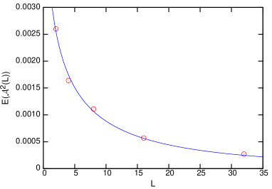
Figure 3: (color online) The second moment of the fitted amplitudes of the power spectrum in a BB potential. Numerical results are shown as circles along with the fit of the data by $a\exp(-L^{b})$, shown as a solid line, yielding the fitted value $b=0.37$

Before we proceed to the analysis of the distribution of the amplitude ${\cal A}$, two remarks are in order. We first note that there exists another physical system, completely unrelated to the one under study, which exhibits essentially the same behavior. It concerns survival of diffusing particles, with diffusion coefficient $D_{V}$, in presence of perfect traps, independently and uniformly distributed on a one-dimensional line. Identifying $L$ as time and $1/T$ as the density of traps, we see that in one-dimensional systems the behavior of the moments of the probability $S_{L}$ that a particle survives up to time $L$ is identical to the behavior of the moments of ${\cal A}$ (see, e.g., yuste and references therein). At sufficiently short times $L$, $S_{L}$ follows the stretched-exponential form in (19), which is tantamount to the so-called Smoluchowski regime, while for $L\to\infty$, the moments of $S_{L}$ obey the form in (31) as they are supported by the optimal fluctuation $R^{*}=(TV_{0}^{2}L/k)^{1/3}$ of a random cavity devoid of traps. This ultimate, late time, regime has the celebrated fluctuation-induced tails bal ; don , which are also intimately related to the so-called Lifshitz singularity in the low-energy spectrum of an electron in a one-dimensional disordered array of scatterers lifsh . Below we will show that an analogous essential singularity shows up in the distribution $P({\cal A})$.

Secondly, we are now in position to estimate the crossover time $t_{c}$, and hence, to determine the upper bound on the frequency for which the spectrum (2) is characterized by an exponent $\alpha=2$. Recalling that our numerical results show a sharp crossover from the Sinai regime (3) to the diffusive behavior in (9), we may estimate $t_{c}$ by simply equating the mean squared displacement in the Sinai (3) and diffusive regimes (9), i.e.

$$\ln^{4}(t_{c})\sim\mathbb{E}\left(D[V(x)]\right)\,t_{c}\,,$$ (32)

which gives

$$t_{c}\sim\dfrac{1}{\mathbb{E}\left(D[V(x)]\right)}\,.$$ (33)

Now noticing that $D[V(x)]\sim{\cal A}$, we can expect that $t_{c}$ will display a different dependence on the periodicity $L$ (and the other system parameters) for small and large values of $L$. For sufficiently small $L$ (but still large enough so that the behavior in (3) has enough space to emerge), the typical trajectories of disorder, such that $|V(x)|\sim\sqrt{x}$, will dominate and

$$t_{c}\sim\exp\left(\dfrac{V_{0}}{T}L^{1/2}\right)\,,$$ (34)

which simply tells us that, for sufficiently small $L$, the crossover time $t_{c}$ to diffusive regime is a time needed for $x(t)$ to travel over a distance $L$ encountering a typical barrier $V_{0}L^{1/2}$ which $x(t)$ overcomes due to thermal activation. Note the Arrhenius dependence of $t_{c}$ on the temperature $T$.

For larger values of $L$ the behavior of the average amplitude ${\cal A}$, given by Eq. (31), becomes supported by atypical realizations of disorder with the optimal fluctuation trajectories of $|V(x)|\sim x^{1/3}$. For such $L$, we have, by virtue of (31),

$$t_{c}\sim\exp\left(c\left(\dfrac{V_{0}}{T}\right)^{2/3}L^{1/3}\right)\,,$$ (35)

where $c$ is a numerical constant; this means that, for larger periodicities, $t_{c}$ exhibits a slower growth with $L$. Note that in this case $t_{c}$ has a rather unusual sub-Arrhenius dependence on the temperature.

In order to discuss this point and to use our numerical data to better understand it, we start by defining a time of exit from the Sinai asymptotic regime. The Sinai regime holds in the first part of the dynamical evolution. We define an exit time from it as the time $t_{c}^{(1)}$ as the minimal time such that

$$\mathbb{E}\left(\overline{|x(t)|}\right)-\mathbb{E}\left(\overline{|x(t)|}\right)_{Sinai}>3\sigma_{Sinai}(t)\;,$$ (36)

where by the $Sinai$ label we denote an average over the motion in an infinite, unconstrained Sinai potential. In this way we are observing the time where the departure of the motion in the periodic Brownian Bridge potential is substantially different from the one in a Sinai infinite potential ($\sigma_{Sinai}$ is the standard deviation over our numerical estimate for the infinite Sinai motion). On our time scales and sample size this procedure is accurate enough to give a sensible estimate of $t_{c}^{(1)}$. We assume now that

$$\ln(t_{c}^{(1)})\sim a^{(1)}+L^{b^{(1)}}\;.$$ (37)

Since our numerical data are not accurate enough to allow us to disentangle precisely the subleading corrections to this behavior, we analyze our data by defining a size dependent exponent $b^{(1)}(L,2L)$, computed by using Eq. (37) for size $L$ and size $2L$. The numerical values computed for $t_{c}^{(1)}(L)$ and the one for $t_{c}^{(1)}(2L)$ are used to disentangle the value of $b^{(1)}(L,2L)$ as estimated from these two values of the lattice size. The limit for large $L$ of $b^{(1)}(L,2L)$ is $b^{(1)}$.

We plot this estimated exponent as a function of $L$ in Fig. 4. In this case the crossover we have derived analytically clearly emerges from the numerical data, that give an estimated exponent close to $1/2$ for small $L$ values and close to $1/3$ for larger values of the size $L$.

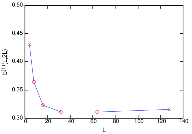
Figure 4: (color online) The exponent $b^{(1)}(L,2L)$ in Eq.(37) as a function of $L$.

We finally turn to the analysis of the distribution $P({\cal A})$ of the amplitude of the low-frequency power spectrum (see Fig. 5). Examining first the negative moments of ${\cal A}$, we observe that they are growing functions of $L$ and $k$, which hints that such a behavior of ${\cal A}$ is derived from the left-tail of the distribution $P({\cal A})$, i.e., when ${\cal A}$ is close to $0$. Furthermore, the quadratic dependence of the moments on the order of the moment $k$ in the exponential is a fingerprint of the log-normal distribution, which suggest that the left-tail of $P({\cal A})$ has the form:

$$P({\cal A})\sim\dfrac{1}{{\cal A}}\exp\left(-\dfrac{2T^{2}\ln^{2}\left({\cal A}\right)}{V_{0}^{2}L}\right)\,.$$ (38)

Note that this distribution is uni-modal, with the most probable value of ${\cal A}_{mp}\sim\exp(-V_{0}^{2}L/4T^{2})$, which is, for sufficiently large $L$, much smaller and closer to $0$ than the typical value in (19).

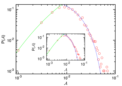
Figure 5: (color online) Distribution $P({\cal A})$ of the amplitudes ${\cal A}$ for a BB potential, plotted with circles (numerical results). In the main figure $L=64$ while the inset shows the results for $L=32$. The log-normal fit corresponding to Eq. (38) is shown for small ${\cal A}$ as a solid green curve while the prediction of Eq. (46) for the right tail is shown for large values of ${\cal A}$ by the dashed blue line.

Further on, positive moments in (31) are, for large $L$, much larger than those expected from the typical realizations of disorder, (19). This means, in turn, that the behavior in (31) stems apparently from the right-tail of the distribution $P(\cal A)$ when ${\cal A}$ is close to the right edge of the support, i.e., ${\cal A}\approx A_{r}=4D_{0}$. Let us formally write

$$\int^{4D_{0}}_{0}{\cal A}^{k}d{\cal A}\,P({\cal A})\sim A_{r}^{k}\,\exp\left(-\left(\dfrac{kV_{0}\sqrt{L}}{T}\right)^{2/3}\right)\,,$$ (39)

where for simplicity of notation any numerical constant in the exponential of the right hand side is included in $V_{0}$. We assume that the major contribution to the integral on the left hand side of (39) comes from a narrow region close to the right edge of the support. Changing the integration variable as

$$z=\dfrac{T}{V_{0}\sqrt{L}}\ln\left(\dfrac{A_{r}}{{\cal A}}\right)\,,$$ (40)

we cast (39) into the form

$$\dfrac{4D_{0}V_{0}\sqrt{L}}{T}\int^{\infty}_{0}dz\,\exp\left(-\left(\dfrac{kV_{0}\sqrt{L}}{T}\right)z\right)\,\times$$

$$\exp\left(-\dfrac{V_{0}\sqrt{L}z}{T}\right)\,P(z)\sim\exp\left(-\left(\dfrac{kV_{0}\sqrt{L}}{T}\right)^{2/3}\right)\,.$$ (41)

Using then the formal definition of the Laplace transform of one-sided stable Lévy distribution ${\cal L}_{\nu}(z)$ with index $\nu$ (see, e.g., greg )

$$\int^{\infty}_{0}\exp\left(-pz\right){\cal L}_{\nu}(z)\equiv\exp\left(-p^{\nu}\right)$$ (42)

we immediately infer that

$$P({\cal A})\sim\dfrac{T}{V_{0}\sqrt{L}{\cal A}}{\cal L}_{2/3}\left(\dfrac{T}{V_{0}\sqrt{L}}\ln\left(\dfrac{A_{r}}{{\cal A}}\right)\right)\,.$$ (43)

Note that the result in (43) is expected to hold only in the vicinity of the right edge of the support, and we consider its asymptotic form in this domain. For ${\cal A}\approx A_{r}$, the argument $z$ in the one-sided Lévy distribution ${\cal L}_{2/3}(z)$ is close to zero, so that its asymptotic behavior is given by

$${\cal L}_{2/3}(z)\sim z^{-2}\exp\left(-\dfrac{b}{z^{2}}\right)\,,$$ (44)

where $b$ is a computable constant. For ${\cal A}\approx A_{r}$, we have that

$$z\approx\dfrac{T}{V_{0}\sqrt{L}}\left(1-\dfrac{{\cal A}}{A_{r}}\right)\,,$$ (45)

so that eventually we find the following asymptotic representation of the distribution $P({\cal A})$ close to the right edge of the support

$$P({\cal A})\sim\dfrac{4D_{0}V_{0}\sqrt{L}}{\left(4D_{0}-{\cal A}\right)^{2}}\exp\left(-\left(\dfrac{4D_{0}V_{0}\sqrt{bL}}{T\left(4D_{0}-{\cal A}\right)}\right)^{2}\right)\,.$$ (46)

Note that the distribution in (46) exhibits an essential singularity in the vicinity of $A_{r}$, which is related to the Lifshitz singularity. In Fig. 5 we plot the empirical probability distribution obtained in numerical simulations, together with the best fits to the asymptotic forms (38) and (46): the agreement is remarkable.

EM and GO wish to thank the Kavli Institute for Theoretical Physics of the University of California at Santa Barbara for warm hospitality during their participation in March 2014 at the program Active Matter: Cytoskeleton, Cells, Tissues and Flocks, where this work has been initiated. DSD and GO acknowledge a partial support from the Office of Naval Research Global Grant N62909-15-1-C076 and also thank the Institute for Mathematical Sciences of the National University of Singapore for warm hospitality and a financial support. EM has used towards development of this project funding from the European Research Council (ERC) under the European Union’s Horizon 2020 research and innovation programme (grant agreement No [694925]).

References

- (1) B. Mandelbrot, Some noises with spectrum, a bridge between current and white noise, IEEE Trans. Inf. Theory 13, 289 (1967)
- (2) P. Dutta and P. M. Horn, Low-frequency fluctuations in solids: noise, Rev. Mod. Phys. 53, 497 (1981).
- (3) O. Bénichou, P.L. Krapivsky, C. Mejia-Monasterio and G. Oshanin, Temporal correlations of the running maximum of a Brownian trajectory, arXiv:1602.06770v2
- (4) A. Sornette and D. Sornette, Europhys. Lett. 9, 197 (1989).
- (5) B. B. Mandelbrot and J. R. Wallis, Water Resour. Res. 5, 321 (1969).
- (6) J. M. Halley, Ecology, evolution and noise, Trends Ecology Evol. 11, 33 (1996).
- (7) D. L. Gilden, T. Thornton and M. W. Mallon, Science 267, 1837 (1995).
- (8) I. Csabai, J. Phys. A: Math. Theor 27, L417 (1994).
- (9) W. H. Press, Comments Astrophys. Space Phys. 7, 103 (1978).
- (10) S. M. Bezrukov and M. Winterhalter, Phys. Rev. Lett. 85, 202 (2000).
- (11) Z. Siwy and A. Fulinski, Phys. Rev. Lett. 89, 1 (2002).
- (12) D. Krapf, Phys. Chem. Chem. Phys. 15, 459 (2013).
- (13) A. R. Bizzarri and S. Cannistrato, Phys. Rev. Lett. 110, 048104 (2013).
- (14) S. Sadegh, E. Barkai and D. Krapf, New J. Phys. 16, 113054 (2014).
- (15) E. Marinari, G. Parisi, D. Ruelle, and P. Windey, Phys. Rev. Lett. 50, 1223 (1983).
- (16) E. Marinari, G. Parisi, D. Ruelle, and P. Windey, Commun. Math. Phys. 89, 1 (1983).
- (17) E. W. Montroll and M. F. Shlesinger, Proc. Natl. Acad. Sci. USA 79, 3380 (1982).
- (18) M. Niemann, H. Kantz and E. Barkai, Phys. Rev. Lett. 110, 140603 (2013).
- (19) N. Leibovitch and E. Barkai, Phys. Rev. Lett. 115, 080602 (2015).
- (20) Ya. G. Sinai, Theor. Probab. Appl. 27, 256 (1982).
- (21) J-P Bouchaud, A. Comtet, A. Georges and P. Le Doussal, Ann. Phys. 201, 285 (1990).
- (22) S. F. Burlatsky, G. Oshanin, A. Mogutov and M. Moreau, Phys. Rev. A 45, R6955 (1992).
- (23) G. Oshanin, A. Mogutov and M. Moreau, J. Stat. Phys. 73, 379 (1993).
- (24) C. Monthus and A. Comtet, J. Physique I France 4, 635 (1994).
- (25) G. Oshanin, A. Rosso and G. Schehr, Phys. Rev. Lett. 110, 100602 (2013).
- (26) A. Comtet and D. S. Dean, J. Phys. A 31, 8595 (1998).
- (27) G. Oshanin and S. Redner, Europhys. Lett. 85, 10008 (2009).
- (28) D. S. Dean, S. Gupta, G. Oshanin, A. Rosso and G. Schehr, J. Phys. A: Math. Theor 47, 372001 (2014).
- (29) P. Mörters and Y. Peres, Brownian motion, (Cambridge: Cambridge University Press, 2010).
- (30) S. Lifson and J. L. Jackson, J. Chem. Phys. 36, 2410 (1962).
- (31) R. Festa and E. Galleani d’Agliano, Physica A 90, 229 (1978)
- (32) P. Reimann, C. van den Broeck, H. Linke, P. Hänggi, J. M. Rubi and A. Pérez-Madrid, Phys. Rev. Lett. 87, 010602 (2001); Phys. Rev. E 65, 031104 (2002).
- (33) D. S. Dean and C. Touya, J. Phys. A: Math. Theor. 41, 335002 (2009).
- (34) O. Bénichou, P.L. Krapivsky, C. Mejia-Monasterio and G. Oshanin, J. Phys. A, to appear
- (35) A. N. Kolmogorov, Giorn. Inst. Ital. Attuari 4, 83 (1933).
- (36) N. V. Smirnov, Bull. Math. Univ. Moscou 2, 2 (1939)
- (37) W. Feller, Ann. Math. Stat. 19, 177 (1948).
- (38) C. Monthus, G. Oshanin, A. Comtet and S. F. Burlatsky, Phys. Rev. E 54, 231 (1996).
- (39) W. Feller, Ann. Math. Stat. 22, 427 (1951).
- (40) D. P. Kennedy, J. Appl. Probab. 13, 371 (1976).
- (41) S. N. Majumdar, J. Randon-Furling, M. J. Kearney and M. Yor, J. Phys. A: Math. Theor. 41, 365005 (2008).
- (42) S. B. Yuste, G. Oshanin, K. Lindenberg, O. Benichou and J. Klafter, Phys. Rev. E 78, 021105 (2008).
- (43) B. Ya. Balagurov and V. G. Vaks, Sov. Phys. JETP 38, 968 (1974).
- (44) M. D. Donsker and S. R. S. Varadhan, Commun. Pure Appl. Math. 28, 525 (1975); ibid 32, 721 (1979).
- (45) I. M. Lifshitz, Sov. Phys. JETP 17, 1159 (1963); Sov. Phys. Usp. 7, 549 (1965).
- (46) G. Schehr and P. Le Doussal, J. Stat. Mech. P01009 (2010).