Tensor Network Skeletonization

Abstract.

We introduce a new coarse-graining algorithm, tensor network skeletonization, for the numerical computation of tensor networks. This approach utilizes a structure-preserving skeletonization procedure to remove short-range correlations effectively at every scale. This approach is first presented in the setting of 2D statistical Ising model and is then extended to higher dimensional tensor networks and disordered systems. When applied to the Euclidean path integral formulation, this approach also gives rise to new efficient representations of the ground states for 1D and 2D quantum Ising models.

1. Introduction

This paper is concerned with the numerical computation of tensor networks (see [Orus2014] for a good introduction for tensor networks). Recently, tensor networks have received a lot of attention in computational statistical mechanics and quantum mechanics as they offer a convenient and effective framework for representing

• the partition functions for the classical spin systems in statistical mechanics and

• the ground and thermal states of quantum many body systems through the Euclidean path integral formulation.

1.1. Definition

A tensor network is associated with a triple $(V,E,\{T^{i}\}_{i\in V})$ where $V$ is a set of vertices, $E$ is a set of edges, and $T^{i}$ is a tensor at vertex $i\in V$.

• The degree of the vertex $i\in V$ is denoted as $d_{i}$.

• Each edge $e\in E$ is associated with a bond dimension $\chi_{e}$.

• For each vertex $i\in V$, $T^{i}$ is a $d_{i}$-tensor. Each of the $d_{i}$ components of $T^{i}$ is associated with one of the adjacent edges of the vertex $i$ and the dimension of this component is equal to the bond dimension of the associated edge.

The edge set $E$ can often be partitioned as the disjoint union $E=E_{I}\cup E_{B}$, where $E_{I}$ is the set of the interior edges that link two vertices in $V$ and $E_{B}$ is the set of the boundary edges with one endpoint in $V$ and the other one open. Once the triple $(V,E,\{T^{i}\}_{i\in V})$ is specified, the tensor network represents a tensor that is obtained via contracting all interior edges in $E_{I}$. The result is an $|E_{B}|$-tensor and is denoted as

(1) $$\operatorname{tr}_{E_{I}}\left(\bigotimes_{i\in V}T^{i}\right).$$

When the set $E_{B}$ is empty, the tensor network contracts to a scalar. Throughout this paper, we follow the following notation conventions.

• The lower-case letters such as $i$ and $j$ are used to denote vertices in $V$.

• The lower-case letters such as $a$, $b$, $c$, $d$, $e$, and $f$ are used to denote the edges in $E$.

• The upper-case letters such as $T$, $U$, and $V$ are used to denote tensors.

The framework of tensor networks is a powerful tool since mathematically it offers efficient representations for high dimensional functions or probability distributions with certain underlying geometric structures. For example, let us consider the 2D statistical Ising model on a periodic square lattice. The vertex set $V$ consists of the lattice points of an $n\times n$ Cartesian grid, where $N=n\times n$ is the number of vertices. The edge set $E$ consists of the edges between horizontal and vertical neighbors, defined using the periodic boundary condition (see Figure 1(a)). Here $|E|=2N$, $E_{I}=E$, and $E_{B}=\emptyset$.

At temperature $T$, the partition function $Z_{N}(\beta)$ for the inverse temperature $\beta=1/T$ is given by

$$Z_{N}(\beta)=\sum_{\sigma}e^{-\beta H_{N}(\sigma)},\quad H_{N}(\sigma)=-\sum_{(ij)\in E}\sigma_{i}\sigma_{j},$$

where $\sigma=(\sigma_{1},\ldots,\sigma_{N})$ stands for a spin configuration at $N$ vertices with $\sigma_{i}=\pm 1$ and the sum of $\sigma$ is taken over all $2^{N}$ configurations. Here $(ij)$ is the edge between two adjacent vertices $i$ and $j$ and the sum in $H_{N}(\sigma)$ is over these $2N$ edges.

In order to write $Z_{N}(\beta)$ in the form of a tensor network, one approach is to introduce a $2\times 2$ matrix $S$

$$S=\begin{pmatrix}e^{\beta}&e^{-\beta}\\ e^{-\beta}&e^{\beta}\end{pmatrix},$$

which is the multiplicative term in $Z_{N}(\beta)$ associated with an edge between any two adjacent vertices. The partition function $Z_{N}(\beta)$ is built from the $S$ matrices over all edges in $E$ (see Figure 1(b)). Since $S$ is a symmetric matrix, its symmetric square root $S^{1/2}$ is well defined with the following element-wise identity:

$$S_{ij}=\sum_{a}S^{1/2}_{ia}S^{1/2}_{aj}$$

where $a$ denotes the edge that connects $i$ and $j$ (see Figure 1(c)). Here and throughout the paper, the lower-case letters (e.g. $i$, $j$, and $k$) for denoting a vertex in $V$ are also used for the running index associated with that vertex. The same applies to the edges: the lower-case letters (e.g. $e$ and $f$) for denoting an edge in $E$ are also used as the running index associated with that edge.

At each vertex $i$, one can then introduce a $4$-tensor $T^{i}$

(2) $$T^{i}_{abcd}=\sum_{i}S^{1/2}_{ia}S^{1/2}_{ib}S^{1/2}_{ic}S^{1/2}_{id},$$

which essentially contracts the four $S^{1/2}$ tensors adjacent to the vertex $i$ (see Figure 1(c)). Finally, the partition function $Z_{N}(\beta)$ can be written as

$$Z_{N}(\beta)=\operatorname{tr}_{E}\left(\bigotimes_{i\in V}T^{i}\right)$$

(see Figure 1(d)).

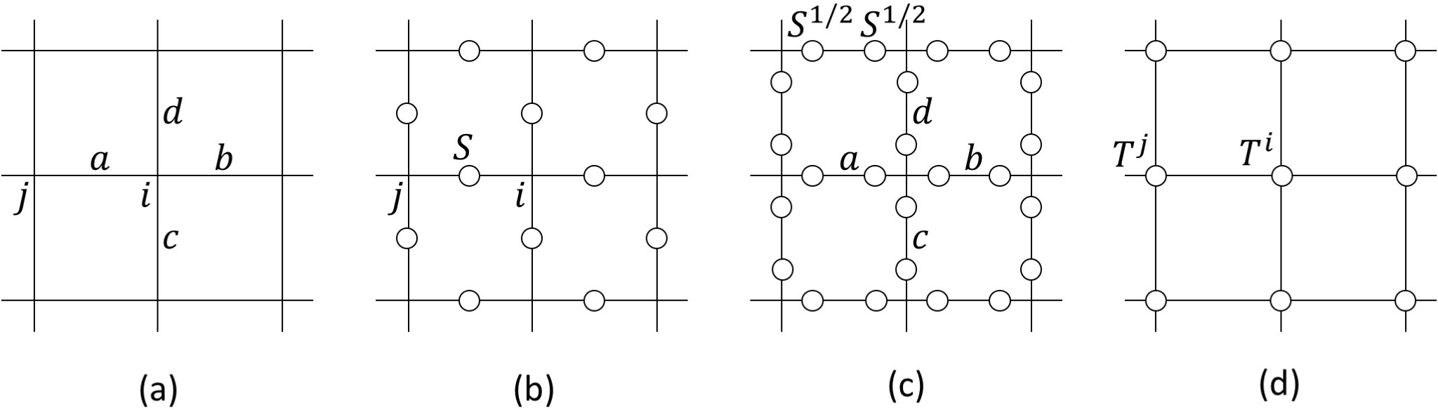
Figure 1. Representing the partition function $Z_{N}(\beta)$ of 2D statistical Ising model using a tensor network. (a) The vertices and edges of the tensor network. (b) The 2-tensor $S$ associated with each edge. (c) Introducing $S^{1/2}$ splits $S$ into the product of two 2-tensors. (d) Contracting the four 2-tensors adjacent to a vertex $i$ forms the 4-tensor $T^{i}$.

1.2. Previous work

One of the main computational tasks is how to evaluate tensor networks accurately and efficiently. The naive tensor contraction following the definition (1) is computationally prohibitive since its running time grows exponentially with the number of vertices.

In recent years, there has been a lot of work devoted to efficient algorithms for evaluating tensor networks. In [Levin2007], Levin and Nave introduced the tensor renormalization group (TRG) as probably the first practical algorithm for this task. When applied to the 2D statistical Ising models, this method utilizes an alternating sequence of tensor contractions and singular value decompositions. However, one problem with TRG is the accumulation of short-range correlation, which increases the bond dimensions and computational costs dramatically as the method proceeds.

In a series of papers [Xie2009, Xie2012, Zhao2010], Xiang et al introduced the higher order tensor renormalization group (HOTRG) as an extension of TRG to address 3D classical spin systems. The same group has also introduced the second renormalization group (SRG) based on the idea of approximating the environment of a local tensor before performing reductions. SRG typically gives more accurate results. However, the computation time of SRG tends to grow significantly with the size of the local environment and it is also not clear how to generalize this technique to systems that are not translationally invariant.

In [Gu2009], Gu and Wen introduced the method of tensor entanglement filtering renormalization (TEFR) as an improvement of TRG for 2D systems. Comparing with TRG, this method makes an extra effort in removing short-range correlations and hence produces more accurate and efficient computations.

More recently in [Evenbly2015, Evenbly2015B], Evenbly and Vidal proposed the tensor network renormalization (TNR). The key step of TNR is to apply the disentanglers to remove short-range correlation. These disentanglers appeared earlier in the work of the multiscale entanglement renormalization ansatz (MERA) [Vidal2008]. For a fixed bond dimension, TNR gives significantly more accurate results compared to TRG, but at the cost of increasing the computational complexity. However, it is not clear how to extend the approach of TNR to systems in higher dimensions.

These approaches have significantly improved the efficiency and accuracy of the computation of tensor networks. From a computational point of view, it would be great to have a general algorithm that have the following three properties:

• removing the short-range correlation efficiently in order to keep bond dimension and computational cost under control, and

• extending to 3D and 4D tensor networks, and

• extending to systems that are not translationally invariant, such as disordered systems.

However, as far as we know, none of these methods achieves all three properties simultaneously.

1.3. Contribution and outline

Building on top of the previous work in the physics literature, we introduce a new coarse-graining approach, called the tensor network skeletonization (TNS), as a first step towards building such a general algorithm. At the heart of this approach is a new procedure called the structure-preserving skeletonization, which removes short-range correlation efficiently while maintaining the structure of a local tensor network. This allows us to generalize TNS quite straightforwardly to spin systems of higher dimensions. In addition, we also provide a simple and efficient algorithm for performing the structure-preserving skeletonization. This allows for applying TNS efficiently to systems that are not translationally invariant.

The rest of this paper is organized as follows. Section 1 summarizes the basic tools used by the usual tensor network algorithms and introduces the structure-preserving skeletonization. Section 3 is the main part of the paper and explains TNS for 2D statistical Ising model. Section 4 extends the algorithm to 3D statistical Ising model. Section 5 discusses how to build efficient representations of the ground states of 1D and 2D quantum Ising models using TNS. Finally, Section 6 discusses some future work.

2. Basic tools

2.1. Local replacement

The basic building blocks of all tensor network algorithms are local replacements. Suppose that vertex $V$ and edge set $E$ of a tensor network $(V,E,\{T^{i}\}_{i\in V})$ are partitioned as follows

$$V=V_{1}\cup V_{2},\quad E=E_{1}\cup E_{2}\cup E_{12},$$

where $E_{1}$ and $E_{2}$ are the sets of interior edges of $V_{1}$ and $V_{2}$, respectively, and $E_{12}$ is the set of edges that link across $V_{1}$ and $V_{2}$. Such a partition immediately gives an identity

(3) $$\operatorname{tr}_{E}\left(\bigotimes_{i\in V}T^{i}\right)=\operatorname{tr}_{E_{2}\cup E_{12}}\left(\left(\bigotimes_{i\in V_{2}}T^{i}\right)\bigotimes\operatorname{tr}_{E_{1}}\left(\bigotimes_{i\in V_{1}}T^{i}\right)\right).$$

Assume now that there exists another tensor network $B$ for which the following approximation holds

$$B\approx\operatorname{tr}_{E_{1}}\left(\bigotimes_{i\in V_{1}}T^{i}\right)$$

(see Figure 2(a)). Typically $B$ is much simpler in terms of the number of the vertices and/or the bond dimensions of the edges. A local replacement refers to replacing $\operatorname{tr}_{E_{1}}\left(\bigotimes_{i\in V_{1}}T^{i}\right)$ in (3) with $B$ to get a simplified approximation

$$\operatorname{tr}_{E}\left(\bigotimes_{i\in V}T^{i}\right)\approx\operatorname{tr}_{E_{2}\cup E_{12}}\left(\left(\bigotimes_{i\in V_{2}}T^{i}\right)\bigotimes B\right)$$

(see Figure 2(b)). Most algorithms for tensor networks apply different types of local replacements successively until the tensor network is simplified to a scalar or left with only boundary edges.

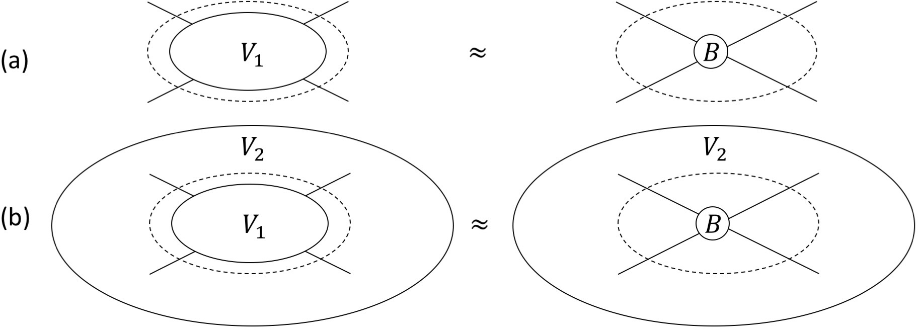
Figure 2. Local replacement. (a) Part of the tensor network associated with vertices in $V_{1}$ is approximated by a simplified tensor network $B$. (b) Locally replacing $V_{1}$ with $B$ results in a approximation of the whole tensor network.

The simplest instance of local replacement is the tensor contraction and it simply combines two adjacent tensors into a single one. For example, let $P$ be a 2-tensor adjacent to edges $a$ and $c$ and $Q$ be another 2-tensor adjacent to edges $c$ and $b$ (see Figure 3(a)). The resulting 2-tensor $T$ obtained from contracting $P$ and $Q$ is simply the product of $P$ and $Q$, i.e.,

$$T_{ab}=\sum_{c}P_{ac}Q_{cb},$$

(see Figure 3(a)). Often when the contraction is applied, the edges $a$ and $b$ typically come from grouping a set of multiple edges.

A second instance is called the projection. Typically it is carried out by performing a singular value decomposition of $T$ followed by thresholding small singular value, i.e.,

$$T\approx USV^{\prime},\quad T_{ab}\approx\sum_{cd}U_{ac}S_{cd}V_{bd}$$

(see Figure 3(b)). Here $U$ and $V$ are both orthogonal matrices and $S$ is a diagonal matrix. Due to the truncation of small singular values, the bond dimensions at edges $c$ and $d$ can be significantly smaller compared to the ones of $a$ and $b$. Throughout this paper, each orthogonal matrix shall be denoted by a diamond in the figures. As with the contraction, each of the indices $a$ and $b$ often comes from grouping a set of multiple edges. The SVD-based projection can also be modified slightly to a few equivalent forms (see Figure 3(b))

$$T\approx UU^{\prime}T,\quad T_{ab}\approx\sum_{ce}U_{ac}U_{ec}T_{eb}$$

$$T\approx UR,\quad R=U^{\prime}T,\quad T_{ab}\approx\sum_{c}U_{ac}R_{cb}.$$

In the rest of this paper, we refer to the first one as the $UU^{\prime}T$-projection and the second one as the $UR$-projection.

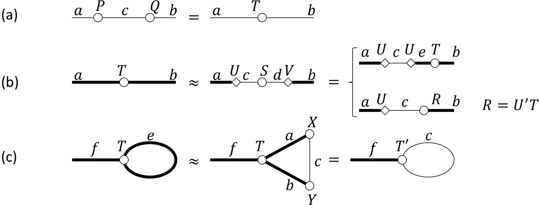
Figure 3. Instances of local replacements. (a) Contraction. (b) Projection. (c) Structure-preserving skeletonization.

Another instance of local replacements uses the disentanglers introduced in [Vidal2008] and it plays a key role in the work of tensor network renormalization (TNR) [Evenbly2015] as mentioned above. Since the tensor network skeletonization (TNS) approach of this paper does not depend on the disentanglers, we refer to the references [Evenbly2015, Vidal2007, Evenbly2009] for more detailed discussions of them.

2.2. Structure-preserving skeletonization

At the center of the TNS approach is a new type of local replacement called the structure-preserving skeletonization. The overall goal is to reduce the bond dimensions of the interior edges of a loopy local tensor network without changing its topology. In the simplest setting, consider a 3-tensor $T$ with two of its components marked with a same edge $e$ (and thus to be contracted). The structure-preserving skeletonization seeks two 2-tensors $X$ and $Y$ (see Figure 3(c)) such that

(4) $$\operatorname{tr}_{e}T\approx\operatorname{tr}_{abc}(X\otimes T\otimes Y),\quad\sum_{e}T_{eef}\approx\sum_{abc}X_{ac}T_{abf}Y_{bc},$$

and also the bond dimension of edge $c$ should be significantly smaller compared to the bond dimension of edge $e$. This is possible because there might exists short-range correlations within the loop that can be removed from the viewpoint of the exterior of this local tensor network.

A convenient way to reformulate the problem is to view $T$ as a $\chi_{e}\times\chi_{e}$ matrix with each entry $T_{ab}$ equal to a $\chi_{f}$-dimensional vector and view $X$ and $Y$ as matrices. Then one can rewrite the condition in (4) as

(5) $$\operatorname{tr}_{e}T\approx\operatorname{tr}_{c}(X^{*}TY)$$

where the products between $X$, $T$, and $Y$ are understood as matrix multiplications.

As far as we know, there does not exist a simple and robust numerical linear algebra routine that solve this approximation problem directly. Instead, we propose to solve the following regularized optimization problem

$$\min_{X,Y}\|\operatorname{tr}_{e}T-\operatorname{tr}_{c}(X^{*}TY)\|_{2}^{2}+\alpha(\|X\|_{F}^{2}+\|Y\|_{F}^{2}),$$

where the constant $\alpha$ is a regularization parameter and is typically chosen to be sufficiently small. This optimization problem is non-convex, however it can be solved effectively in practice using the alternating least square algorithm once a good initial guess is available. More precisely, given a initial guess for $X^{(0)}$ and $Y^{(0)}$, one alternates the following two steps for $n=0,1,\ldots$ until convergence

$$X^{(n+1)} =\operatorname{argmin}_{X}\|\operatorname{tr}_{e}T-\operatorname{tr}_{c}(X^{*}TY^{(n)})\|_{2}^{2}+\alpha\|X\|_{F}^{2}$$

$$Y^{(n+1)} =\operatorname{argmin}_{Y}\|\operatorname{tr}_{e}T-\operatorname{tr}_{c}((X^{(n+1)})^{*}TY)\|_{2}^{2}+\alpha\|Y\|_{F}^{2}.$$

Since each of the two steps is a least square problem in $X$ or $Y$, they can be solved efficiently with standard numerical linear algebra routines. The numerical experience shows that, when starting from well-chosen initial guesses, this alternating least square algorithm converges after a small number of iterations to near optimal solutions.

3. TNS for 2D statistical Ising models

We start with a 2D statistical Ising model on an $n\times n$ lattice with the periodic boundary condition. Following the discussion in Section 1, we set the vertex set $V_{0}$ to be an $n\times n$ Cartesian grid. Each vertex $i$ is identified with a tuple $(i_{1},i_{2})$ with $i_{1},i_{2}\in[n]=\{0,1,\ldots,n-1\}$. The edge set $E_{0}$ consists of the edges between horizontal and vertical neighbors of the Cartesian grid modulus periodicity. This setup also gives rise to an $n\times n$ array of plaquettes. If a plaquette has vertex $i=(i_{1},i_{2})$ at its lower-left corner, then we shall index this plaquette with $i=(i_{1},i_{2})$ as well. Here $N=n^{2}$ is the total number of spins and we assume without loss of generality that $n=2^{L}$.

3.1. Partition function

Following the discussion in Section 1, the partition function $Z_{N}(\beta)$ can be represented using a tensor network $(V^{0},E^{0},\{T^{i}\}_{i\in V_{0}})$ where $T^{i}$ are given in (2). Let $\chi$ be a predetermined upper bound for the bond dimension of the edges of the tensor network. One can assume without loss of generality that the bond dimension $\chi_{e}$ for the edge $e\in E^{0}$ is close to this constant $\chi$. When $\chi$ is significantly larger than 2, this can be achieved by contracting each $2$ neighborhood of tensors into a single tensor. For example, when $\chi=4$, one round of such contractions brings $\chi_{e}=\chi=4$.

3.1.1. Algorithm

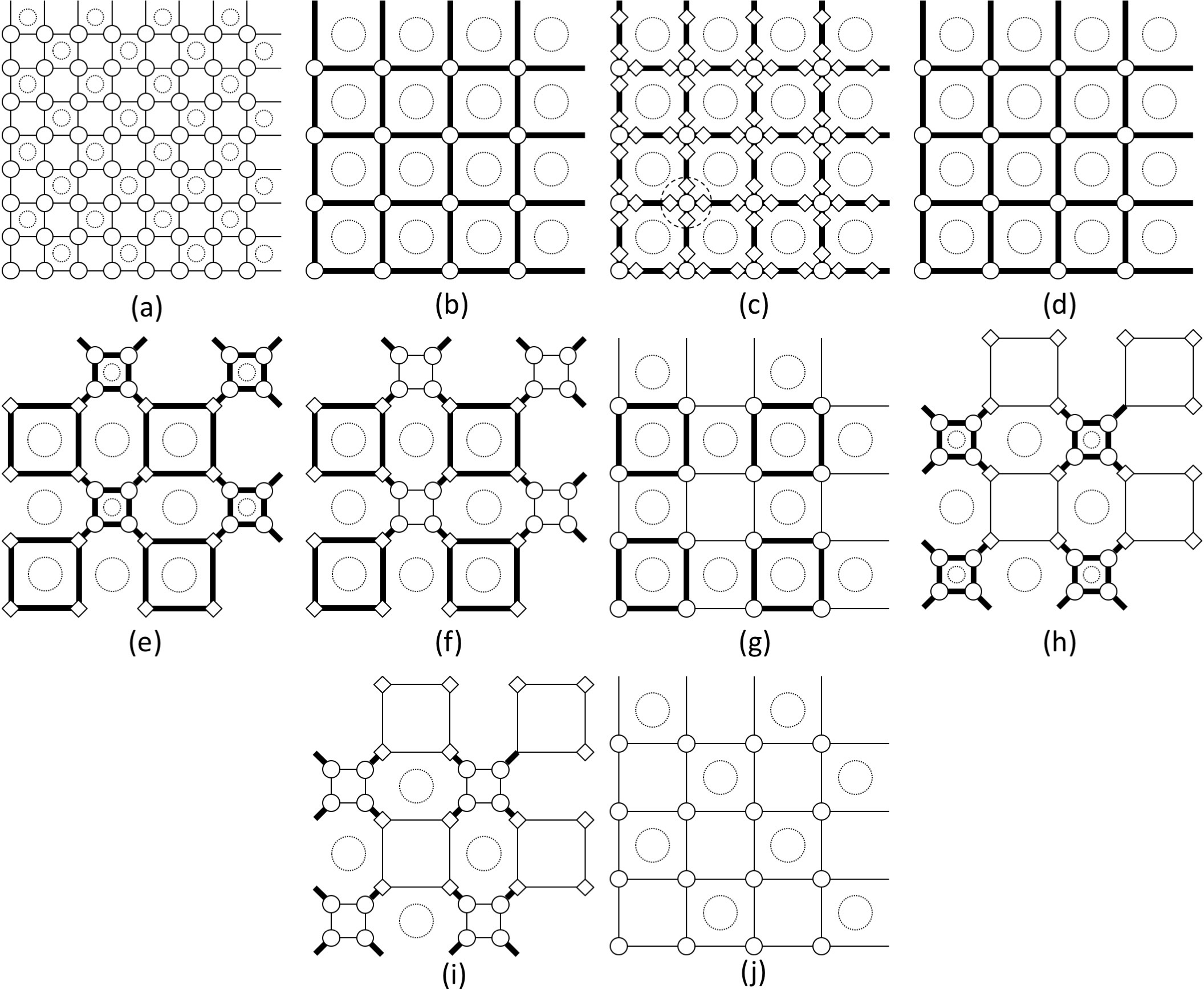
Figure 4. A single iteration of the tensor network skeletonization algorithm. The starting point is a tensor network with bond dimension $\chi$ and short-range correlation removed in the $(0,0)_{2}$ and $(1,1)_{2}$ plaquettes. The final point is a coarse-grained tensor-network with 1/4 vertices (or tensors). This coarse-grained tensor also has bond dimensions equal to $\chi$ and has short-range correlation removed for the (larger) $(0,0)_{2}$ and $(1,1)_{2}$ plaquettes. The bold lines stand for edges with bond dimensions equal to $O(\chi^{2})$.

The TNS algorithm consists of a sequence of coarse-graining iterations. At the beginning of the $\ell$-th iteration, one holds a tensor network $(V^{\ell},E^{\ell},\{T^{i}\}_{i\in V_{\ell}})$ at level $\ell$ with $(n/2^{\ell})\times(n/2^{\ell})$ vertices. With the exception of the $0$-th iteration, we require that the following iteration invariance to hold:

• for each plaquette with index equal to $(0,0)$ or $(1,1)$ modulus 2, the short-range correlation within this plaquette has already been eliminated (see Figure 4(a)).

In what follows, we refer to those plaquettes with index equal to $(0,0)$ modulus 2 as $(0,0)_{2}$ plaquettes and similarly those with index equal to $(1,1)$ modulus 2 as $(1,1)_{2}$ plaquettes. In Figure 4(a), the dotted circles denote the existence of short-range correlation. Notice that these circles do not appear in the $(0,0)_{2}$ plaquettes and $(1,1)_{2}$ plaquettes. The $\ell$-th iteration consists of the following steps.

1. Merge the tensors at the four vertices of each $(0,0)_{2}$ plaquette into a single tensor (see Figure 4(b)). This requires a couple of contractions defined in Section 2. The $(1,1)_{2}$ plaquettes are stretched and this results a new graph that contains only $1/4$ of vertices. The tensors at the new vertices are identical but the bond dimension of the new edges are equal to $\chi^{2}$ (shown using the bold lines). Since these $(1,1)_{2}$ plaquettes at level $\ell$ do not contain short-range correlation at level $\ell$, no short-range correlation of level $\ell$ will survive at level $\ell+1$. However, there are new short-range correlation of level $\ell+1$ in the tensor network and these are marked with larger dotted circles inside the new plaquettes at level $\ell+1$. The key task for the rest of the iteration is to remove part of these short-range correlations at level $\ell+1$ and reduce the bond dimension from $\chi^{2}$ back to $\chi$ at the same time.

2. For each vertex $i$ in Figure 4(b), denote the tensor at $i$ by $T^{i}_{abcd}$ where $a$, $b$, $c$, and $d$ refer to the left, right, bottom, and top edges. Applying two $UU^{\prime}T$-projections (the first one with the left edge vs. the rest and the second one with for the bottom edge vs. the rest) to $T^{i}_{abcd}$ effectively inserts two orthogonal (diamond) matrices in each of these edges (see Figure 4(c)). Most TRG algorithms utilize this step to reduce the bond dimension directly from $\chi^{2}$ back to $\chi$ and thus incurring a significant error. In TNS however, the bond dimension at this point is kept close to $\chi^{2}$. This introduces a much smaller truncation error as compared to the TRG algorithms.

3. At each vertex $i$ in Figure 4(c), merge the tensor $T^{i}_{abcd}$ with the four adjacent orthogonal (diamond) matrices (see Figure 4(d)). Though the tensor network obtained after this step has the same topology as the one in Figure 4(b), the bond dimension is somewhat reduced and one prepares the tensor network for the structure-preserving skeletonization.

4. For each $(1,1)_{2}$ plaquette in Figure 4(d), apply the $UR$-projection to the $4$-tensor at each of its corners. Here the two edges adjacent to the plaquette are grouped together. Notice that the (round) $R$ tensors are placed close to the $(1,1)_{2}$ plaquette while the (diamond) $U$ tensors are placed away from it. Though this projection step does not reduce bond dimensions, it allows us to treat each $(1,1)_{2}$ plaquette separately. The resulting graph is given in Figure 4(e).

5. In this key step, apply the structure-preserving skeletonization to each $(1,1)_{2}$ plaquette. The details of this procedure will be provided below in Section 3.1.2. The resulting $(1,1)_{2}$ plaquette has its short-range correlation removed and the bond dimensions of its four surrounding edges are reduced from $\chi^{2}$ to $\chi$ (see Figure 4(f)).

6. For each $(1,1)_{2}$ plaquette, contract back the $UR$-projections at each of its four corners. Notice that, due to the structure-preserving skeletonizations, the new $R$ tensors have bond dimensions equal to $\chi$. The resulting tensor network (see Figure 4(g)) is similar to the one in Figure 4(d) but now the short-range correlations in the $(1,1)_{2}$ plaquettes are all removed.

7. Now repeat the previous three steps to the $(0,0)_{2}$ plaquettes. This is illustrated in Figure 4(h), (i), and (j). The resulting tensor network now has short-range correlation removed in both $(0,0)_{2}$ and $(1,1)_{2}$ plaquettes. In addition, the bond dimension of the edges is reduced back to $\chi$ from $\chi^{2}$.

This finishes the $\ell$-th iteration. At this point, one obtains a new tensor network denoted by $(V^{\ell+1},E^{\ell+1},\{T^{i}\}_{i\in V_{\ell+1}})$ that is a self-similar and coarse-grained version of $(V^{\ell},E^{\ell},\{T^{i}\}_{i\in V_{\ell}})$. Since the short-range correlations in both $(0,0)_{2}$ and $(1,1)_{2}$ plaquettes are removed, this new tensor network satisfies the iteration invariance and it can serve as the starting point of the $(\ell+1)$-th iteration.

Following this process, the TNS algorithm constructs a sequence of tensor networks

$$(V^{\ell},E^{\ell},\{T^{i}\}_{i\in V_{\ell}}),\quad\ell=0,1,2,\ldots,L.$$

The last one is a single $4$-tensor with the left and right edges identified and similarly with the bottom and top edges identified. Contracting this final tensor gives a scalar value for the partition function $Z_{N}(\beta)$.

3.1.2. Structure-preserving skeletonization

In the description of the algorithm in Section 3.1.1, the missing piece is how to carry out the structure-preserving skeletonization in order to remove the short-range correlation of a $(1,1)_{2}$ plaquette and reduce the bond dimension of its four surrounding edges (from Figure 4(e) to Figure 4(f)).

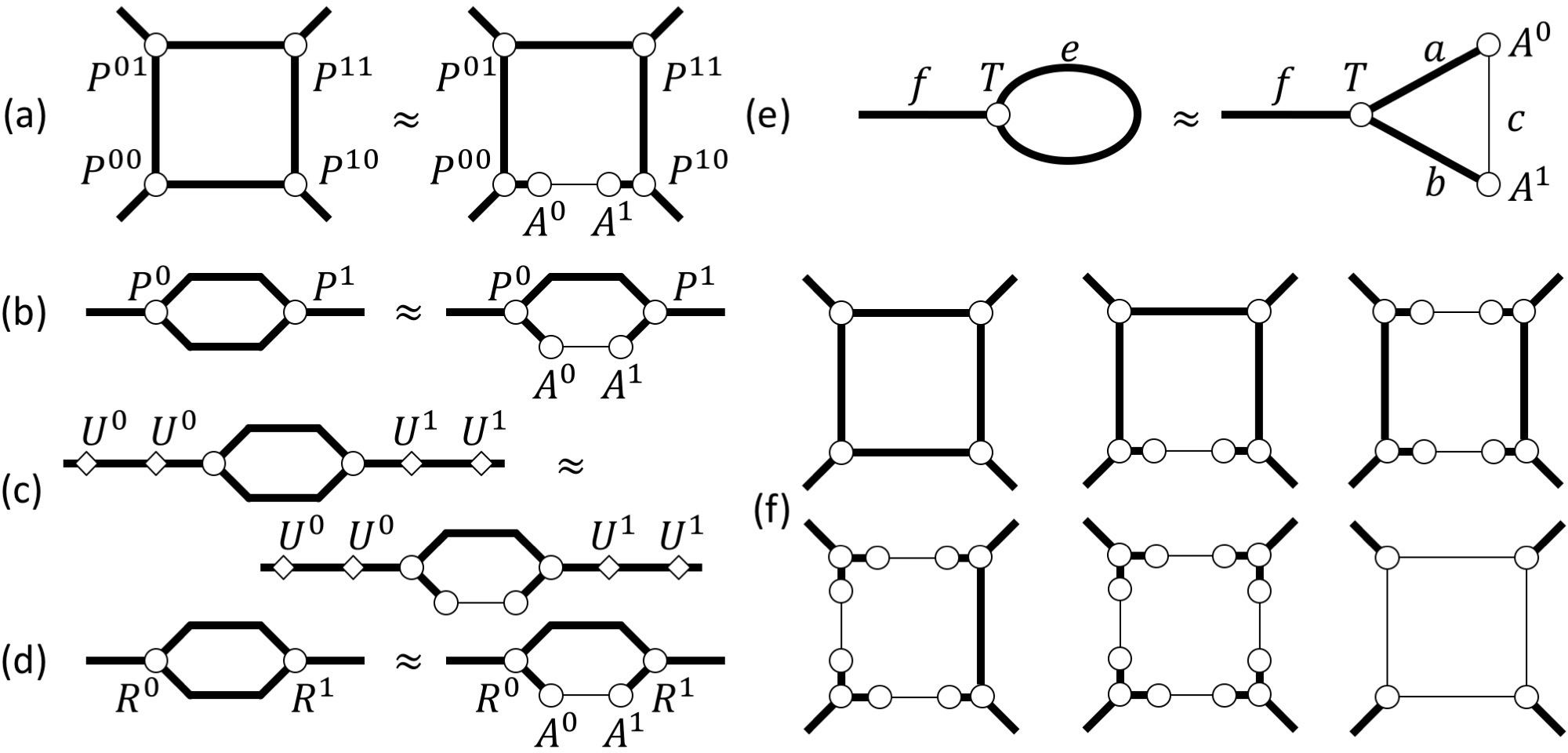
Figure 5. The structure-preserving skeletonization procedure removes the short-range correlation within a $(1,1)_{2}$ (or $(0,0)_{2}$) plaquette. The bold lines stand for edges with bond dimensions $\geq\chi^{2}$.

This procedure is illustrated in Figure 5 with the four corner tensors denoted by $P^{00}$, $P^{10}$, $P^{01}$, and $P^{11}$. Instead of replacing the four corner 3-tensors simultaneously, this procedure considers the 4 interior edges one by one and insert for each edge two tensors of size $\chi^{2}\times\chi$.

1. Starting from the bottom edge, we seek two 2-tensors $A^{0}$ and $A^{1}$ of size $\chi^{2}\times\chi$ under the condition that the 4-tensor represented by the new $(1,1)_{2}$-plaquette (after inserting $A^{0}$ and $A^{1}$) approximates the 4-tensor represented by the original plaquette (see Figure 5(a)).

2. Merge the two left tensors $P^{00}$ and $P^{01}$ into a 3-tensor $P^{0}$ and merge the two right tensors $P^{10}$ and $P^{11}$ into a 3-tensor $P^{1}$. After that, the condition is equivalent to the one given in Figure 5(b). Notice that the two boundary edges have bond dimension equal to $\chi^{4}$.

3. Since the bond dimensions of the two edges between $P^{0}$ and $P^{1}$ will eventually be reduced to $\chi$, this implies that the bond dimensions of the two boundary edges can be cut down to $\chi^{2}=\chi\times\chi$ without affecting the accuracy. For this, we perform the $UU^{\prime}T$-projection to both $P^{0}$ and $P^{1}$. This gives rise the condition in Figure 5(c).

4. Remove the two tensors $U^{0}$ and $U^{1}$ at the two endpoints. Merge $U^{0}$ with $P^{0}$ to obtain a 3-tensor $R^{0}$ and similarly merge $U^{1}$ with $P^{1}$ to obtain a 3-tensor $R^{1}$. The approximation condition can now be written in terms of $R^{0}$ and $R^{1}$ as in Figure 5(d).

5. Finally, contracting the top edge between $R^{0}$ and $R^{1}$ results in a new 3-tensor $T$. The approximation condition now takes the form given in Figure 5(e). This is now exactly the setting visited in Section 2.2 and can be solved efficiently using the alternating least square algorithm proposed there.

At this point, two tensors $A^{0}$ and $A^{1}$ are successfully inserted into the bottom edge. One can repeat this process now for the top, left, and right edges in a sequential order. Once this is done, merging each of the corner tensors with its two adjacent inserted tensors gives the desired approximation (see Figure 5(f) for this whole process).

A task of reducing the bond dimensions of the four surrounding edges of a plaquette has appeared before in the work of tensor entanglement filtering renormalization (TEFR) [Gu2009]. However, the algorithms proposed there are different the one described here and the resulting plaquette was used in a TRG setting that does not extend naturally to higher dimensions tensor network problems.

3.1.3. A modified version

In terms of coarse-graining the tensor network, each iteration of the algorithm in Section 3.1.1 achieves the important goal of constructing a self-similar version while keeping the bond dimension constant (equal to $\chi$) (see Figure 4(a) and (j) for comparison).

However, for the purpose of merely computing the partition function $Z_{N}(\beta)$, a part of the work is redundant. More specifically, at the end of the $\ell$-th iteration, the structure-preserving skeletonization is also performed to the $(0,0)_{2}$-plaquettes at level $\ell+1$ to remove their short-range correlations. However, right at the beginning of the next iteration, a merging step contracts the four corner tensors of each $(0,0)_{2}$-plaquette. By eliminating this structure-preserving skeletonization for the $(0,0)_{2}$ plaquettes, one obtains a modified version of the algorithm (see Figure 6) that can potentially be computationally more efficient.

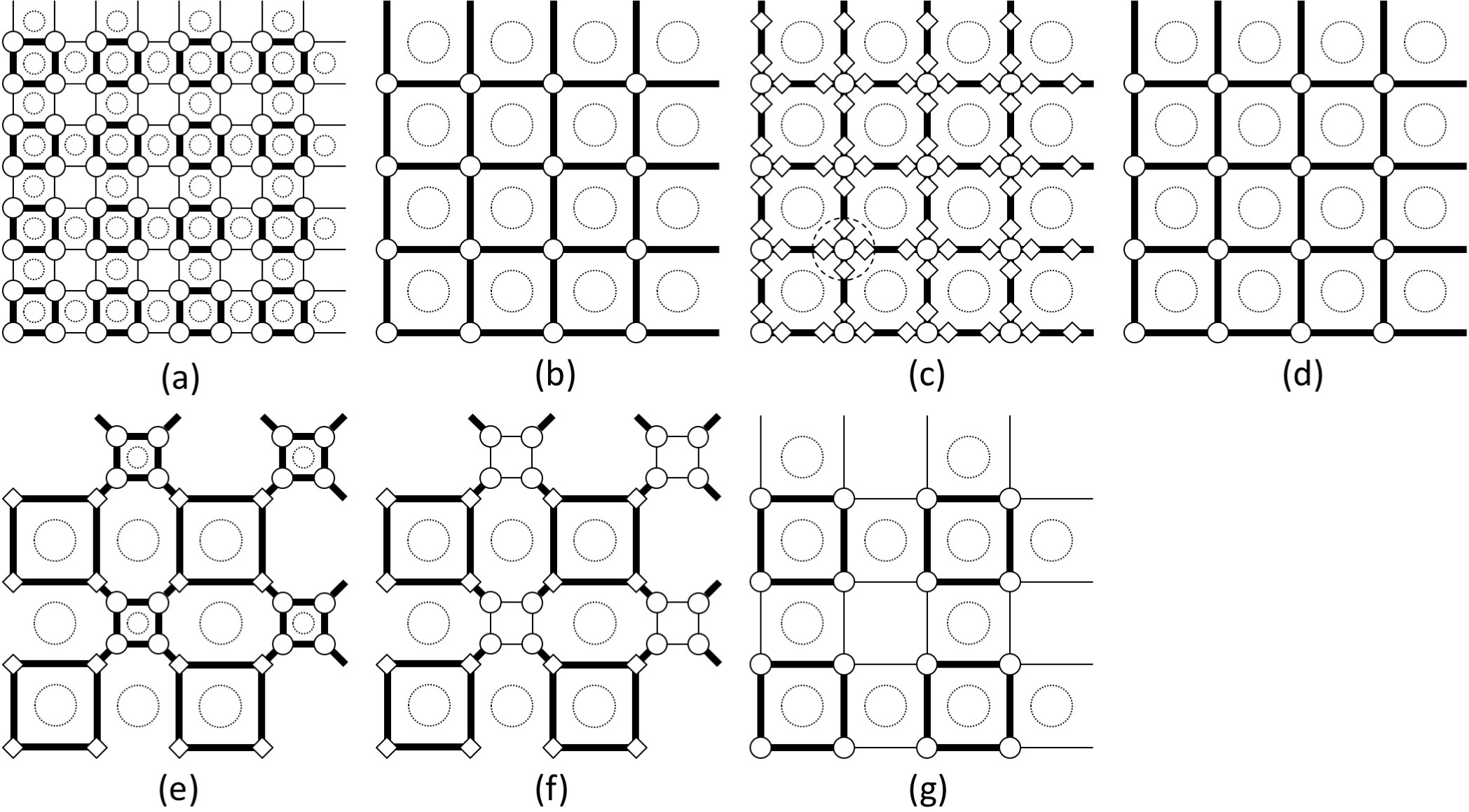
Figure 6. A single iteration of the modified tensor network skeletonization algorithm. The starting point is a tensor network with short-range correlation removed in $(1,1)_{2}$ plaquettes. The final point is a coarse-grained tensor-network with 1/4 vertices (tensors). This coarse-grained tensor also has bond dimensions equal to $\chi$ around the $(1,1)_{2}$ plaquettes and $\chi^{2}$ around the $(0,0)_{2}$ plaquettes. The short-range correlation is removed for the (larger) $(1,1)_{2}$ plaquettes. The bold lines stand for edges with bond dimensions $\chi^{2}$.

Compared with the algorithm illustrated in Figure 4, the main differences are listed as follows

• The iteration invariance is that, at the beginning of each iteration, only the short-range correlations of the $(1,1)_{2}$ plaquettes are removed. Therefore, the bond dimensions of the edges around a $(0,0)_{2}$ plaquette are equal to $\chi^{2}$. This is not so appealing from the viewpoint of approximating a tensor network with minimal bond dimension. However, as one can see from Figure 6(a) to Figure 6(b), a contraction step is applied immediately to these $(0,0)_{2}$ plaquettes so that the high bond dimensions do not affect subsequent computations.

• From Figure 6(e) to Figure 6(f), the structure-preserving skeletonization is only applied to the $(1,1)_{2}$ plaquettes.

• In Figure 6(g), the resulting tensor network at level $\ell+1$ satisfies the new iteration invariance and hence it can serve as the starting point of the next iteration.

As we shall see in Section 3.2.1, this modified algorithm also has the benefit of incurring minimum modification when evaluating observables using the impurity method.

3.1.4. Numerical results

Let us denote by $\tilde{Z}_{N}(\beta)$ the numerical approximation of the partition function $Z_{N}(\beta)$ obtained via TNS. The exact free energy per site $f_{N}(\beta)$ and the approximate free energy per site $\tilde{f}_{N}(\beta)$ are defined by

$$f_{N}(\beta)=\left(-\frac{1}{\beta}\log Z_{N}(\beta)\right)/N,\quad\tilde{f}_{N}(\beta)=\left(-\frac{1}{\beta}\log\tilde{Z}_{N}(\beta)\right)/N.$$

For an infinite 2D statistical Ising system, the free energy per site

$$f(\beta)=\lim_{N\rightarrow\infty}f_{N}(\beta,N)$$

can be derived analytically [Huang1987]. Therefore, for sufficiently large $N$, $f_{N}(\beta,N)$ is well approximated by $f(\beta)$. In order to measure the accuracy of TNS for computing the partition function, we define the relative error

$$\delta f_{N}(\beta)\equiv\frac{|\tilde{f}_{N}(\beta)-f(\beta)|}{|f(\beta)|}\approx\frac{|\tilde{f}_{N}(\beta)-f_{N}(\beta)|}{|f_{N}(\beta)|}.$$

The critical temperature of the 2D statistical Ising model is $T_{c}=1/\ln(1+\sqrt{2})$. For a periodic statistical Ising model on a $2^{15}\times 2^{15}$ lattice, Figure 7 plots the relative error (left) and the running time per iteration (right) for $\chi=2,4$ at different temperatures near the critical temperature $T_{c}$.

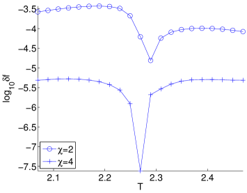
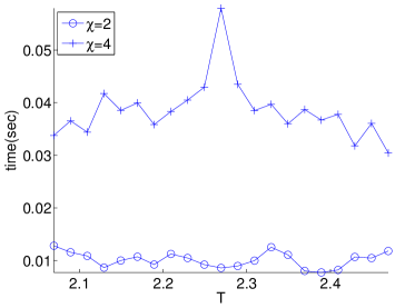
(a)	(b)

Figure 7. Results of free energy calculation. (a) The relative error $\delta f_{N}(\beta)$ of the free energy per site at temperatures around $T_{c}$ for $\chi=2,4$. (b) The running time per iteration of TNS for the same $T$ and $\chi$ values.

From the plots in Figure 7 one can make the following observations.

• First, TNS removes the short-range correlation quite effectively. With $\chi=4$, it achieves 5-6 digits of accuracy for the relative free energy per site. Even with $\chi=2$, one obtains 3-4 digits of accuracy.

• Second, TNS is quite efficiently. For $\chi=4$, each iteration of the TNS takes about 0.05 seconds. The running time tends to grow a bit when $T$ approaches the critical temperature $T_{c}$.

• Most surprisingly, for a fixed $\chi$ value, TNS gives more accurate results when the temperature is close to $T_{c}$. For example with $\chi=4$ and at $T=T_{c}$, the relative error is on the order of $10^{-8}$. This is drastically different from most of the TRG-type algorithms where the accuracy deteriorates significantly near $T_{c}$.

3.2. Observables

The TNS algorithm described in Section 3.1 for computing the partition function (and equivalently the free energy) can be extended to compute observables such as the average magnetization and the internal energy per site.

The internal energy $U_{N}(\beta)$ of the whole system and the internal energy per site $u_{N}(\beta)$ are defined as

$$U_{N}(\beta)=\partial_{\beta}(-\log Z_{N}(\beta))=-\frac{\partial_{\beta}Z_{N}(\beta)}{Z_{N}(\beta)},\quad u_{N}(\beta)=\frac{U_{N}(\beta)}{N}.$$

A direct calculation shows that

$$\partial_{\beta}Z_{N}(\beta)=\sum_{\sigma}e^{-\beta H_{N}(\sigma)}(-H_{N}(\sigma))=\sum_{\sigma}(\sum_{(ij)}\sigma_{i}\sigma_{j})e^{-\beta H_{N}(\sigma)}=N_{e}\sum_{\sigma}(\sigma_{i}\sigma_{j})e^{-\beta H_{N}(\sigma)}$$

where in the last formula $(i,j)$ can be any edge due to the translational invariance of the system and $N_{e}=2N$. This gives the following formula for the internal energy per site

(6) $$u_{N}(\beta)=\frac{U_{N}(\beta)}{N}=\frac{N_{e}}{N}\cdot\frac{\sum_{\sigma}(\sigma_{i}\sigma_{j})e^{-\beta H_{N}(\sigma)}}{\sum_{\sigma}e^{-\beta H_{N}(\sigma)}}=2\frac{\sum_{\sigma}(\sigma_{i}\sigma_{j})e^{-\beta H_{N}(\sigma)}}{\sum_{\sigma}e^{-\beta H_{N}(\sigma)}}.$$

To define the average magnetization, one introduces a small external magnetic field $B$ and defines the partition function of the this perturbed system

$$Z_{N,B}(\beta)=\sum_{\sigma}e^{-\beta H_{N,B}(\sigma)},\quad H_{N,B}(\sigma)=-\left(\sum_{(ij)}\sigma_{i}\sigma_{j}+B\sum_{i}\sigma_{i}\right).$$

The magnetization at a single site $i$ is equal to

(7) $$\left\langle\sigma_{i}\right\rangle_{N,B}(\beta)=\frac{\sum_{\sigma}\sigma_{i}e^{-\beta H_{N,B}(\sigma)}}{\sum_{\sigma}e^{-\beta H_{N,B}(\sigma)}},$$

and the average magnetization $m_{N,B}(\beta)$ is equal to the same quantity since

$$m_{N,B}(\beta)=\frac{1}{N}\sum_{i}\left\langle\sigma_{i}\right\rangle_{N,B}(\beta)=\left\langle\sigma_{i}\right\rangle_{N,B}(\beta),$$

where in the last formulation $i$ can be any site in the periodic Ising model due to the translational invariance of the system.

3.2.1. Algorithm

The computation of the quantities mentioned above requires the evaluation of the following sums:

(8) $$\sum_{\sigma}(\sigma_{i}\sigma_{j})e^{-\beta H_{N}(\sigma)},\quad\sum_{\sigma}\sigma_{i}e^{-\beta H_{N,B}(\sigma)},$$

where $i$ is any site in the first formula while $(i,j)$ is any bond in the second. Both sums can also be represented using tensor networks using the so-called impurity tensor method.

Recall that the 2D periodic statistical Ising model considered here is of size $n\times n$ where $n=2^{L}$. Without loss of generality, one can assume that the sites $i$ and $j$ in (8) are located inside the $2\times 2$ sub-lattice at the center of the whole computation domain. Following the same reasoning in Section 1, one can represent $\sum_{\sigma}(\sigma_{i}\sigma_{j})e^{-\beta H_{N}(\sigma)}$ and $\sum_{\sigma}\sigma_{i}e^{-\beta H_{N,B}(\sigma)}$ as tensor networks. The only difference between them and the tensor network of $Z_{N}(\beta)$ is a single tensor located inside this $2\times 2$ sub-lattice at the center.

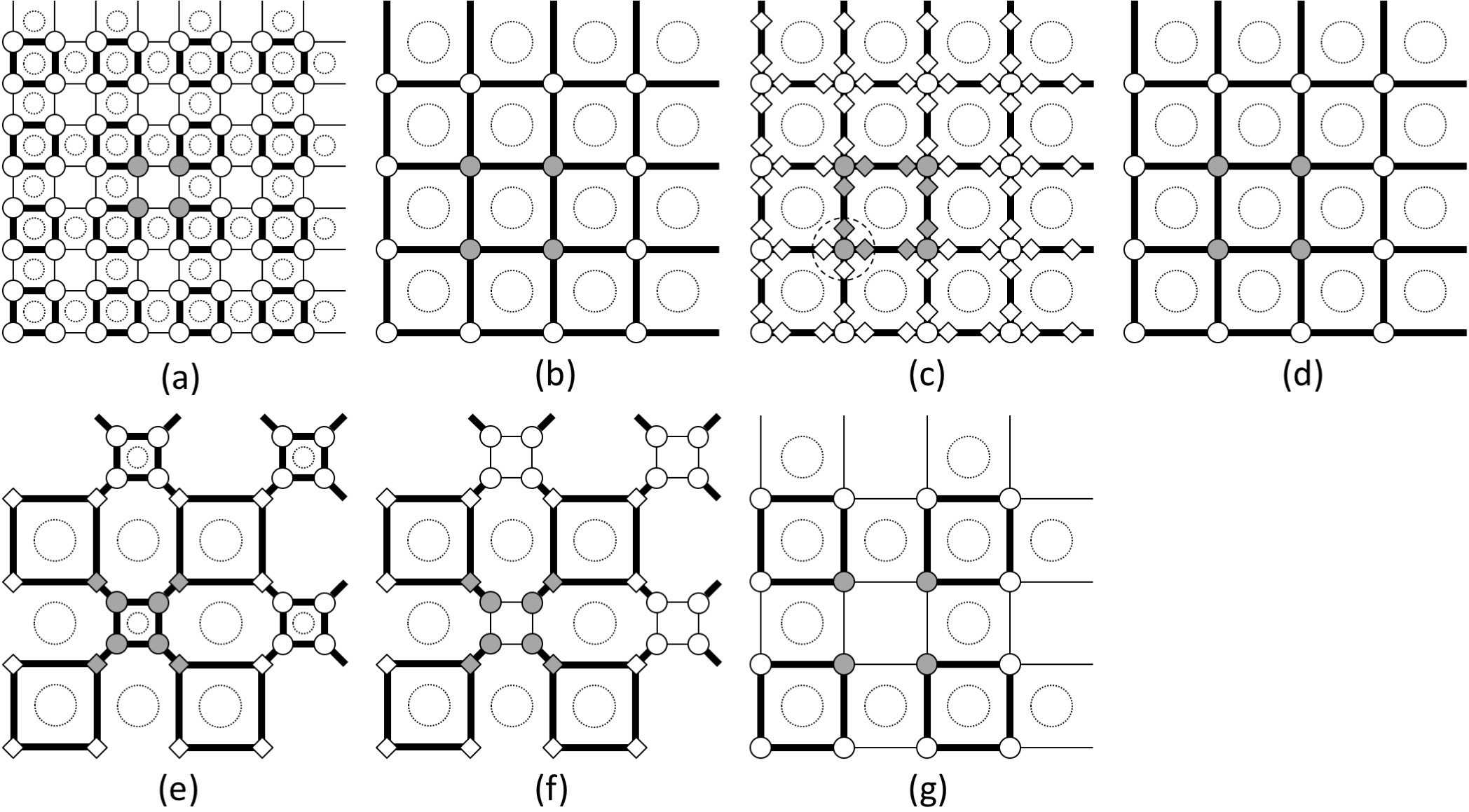
Figure 8. Impurity method for computing the spontaneous magnetization and the internal energy per site. The iteration invariance also requires that at the beginning of each iteration only the four tensors near the center can be different from the ones used in $Z_{N}(\beta)$. These four special tensors are marked in gray. At the end of each iteration, one obtains an coarse-grained tensor network that also satisfies this condition.

The algorithm for computing these new tensor networks are quite similar and it becomes particularly simple when the modified TNS algorithm in Section 3.1.3 is used. The whole algorithm is illustrated in Figure 8 and here we highlight the main differences.

• In addition to the iteration invariance of the modified algorithm in Section 3.1.3, one also requires that only the four tensors at the center (marked in gray in Figure 8(a)) can be different from the ones used for $Z_{N}(\beta)$.

• Because the four special tensors are at the center at the tensor network at level $\ell$, after contraction there are exactly four special tensors at the center of the tensor network at level $\ell+1$ (marked in gray in Figure 8(b)). The rest are identical to the ones used for $Z_{N}(\beta)$.

• From Figure 8(b) to Figure 8(c), the $UU^{\prime}T$-projections at the four surrounding edges of the center plaquette are computed from the four special corner tensors. The resulting orthogonal $U$ matrices are marked in gray as well. The $UU^{\prime}T$-projection at all other edges are inherited from the algorithm for the partition function $Z_{N}(\beta)$. When contracting the tensor at each vertex with its four adjacent orthogonal (diamond) matrices (see Figure 8(c) to Figure 8(d)), this ensures that only the four tensors at the center are different from the ones used for $Z_{N}(\beta)$.

• In the structure-preserving skeletonization step for the $(1,1)_{2}$ plaquettes (see Figure 8(e) and (f)), only the center $(1,1)_{2}$ plaquette is different from the one appeared in $Z_{N}(\beta)$. Therefore, this is the only one that requires an extra structure-preserving skeletonization computation.

• When contracting the tensors at the corners of the $(1,1)_{2}$ plaquettes to get back the 4-tensors in Figure 8(g), again only the four tensors at the center (marked in gray) are different. This ensures that the tensor network at the beginning of the next iteration satisfies the iteration invariance mentioned above.

At each iteration of the in this impurity method, the algorithm performs a constant number of extra $UU^{\prime}T$-projection and one extra structure-preserving skeletonization for the $(1,1)_{2}$ plaquette at the center. When $\chi$ is fixed, all these computation takes a constant number of steps. As a result,the extra computational cost for the impurity method is proportional to $O(L)=O(\log N)$ once the evaluation of $Z_{N}(\beta)$ is ready.

3.2.2. Numerical results

For the internal energy $u_{N}(\beta)$, we denote by $\tilde{u}_{N}(\beta)$ its TNS approximation. When $N$ approaches infinity, the limit

$$u(\beta)=\lim_{N\rightarrow\infty}u_{N}(\beta)$$

can be derived analytically [Huang1987]. Therefore for $N$ sufficiently large, $u(\beta)$ serves as a good benchmark for measuring the accuracy of the TNS algorithm.

For the averaged magnetization, let us denote by $\tilde{m}_{N,B}(\beta)$ the TNS approximation of $m_{N,B}(\beta)$. For the 2D statistical Ising model, the spontaneous magnetization $m_{+}(\beta)$ is defined as

$$m_{+}(\beta)=\lim_{B\rightarrow 0^{+}}\lim_{N\rightarrow\infty}m_{N,B}(\beta)$$

and this can be written down analytically as well [Huang1987, Yang1952]. When $B$ is a small positive number, by setting $N$ to be sufficiently large, one can treat $m_{+}(\beta)$ as a good approximation of $m_{N,B}(\beta)$ and use it as a benchmark for measuring the accuracy of $\tilde{m}_{N,B}(\beta)$.

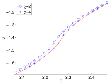
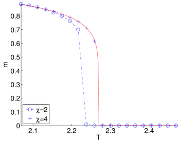
(a)	(b)

Figure 9. Numerical results for computing the observables using the impurity method for $\chi=2,4$. (a) Internal energy. (a) Average magnetization.

Figure 9(a) shows the computed internal energy per site $\tilde{u}_{N}(\beta)$ along with $u(\beta)$ for $\chi=2,4$. On the right, Figure 9(b) gives the computed average magnetization $\tilde{m}_{N,B}(\beta)$ along with the spontaneous magnetization $m_{+}(\beta)$. Though the computation with $\chi=2$ has a significant error, it does exhibit the phase-transition clearly. Once $\chi$ is increased to 4, the numerical results and the exact curves match very well.

3.3. Extension to disordered systems

The tensor network skeletonization algorithm can also be extended easily to disordered systems and we briefly sketch how this can be done. For example, consider the 2D Edwards-Anderson spin-glass model (see [Nishimori2001] for example) where the spins are arranged geometrically the same fashion as the classical Ising model but each edge $(i,j)$ is associated with a parameter $J_{ij}$. For a fixed realization of $J\equiv\{J_{ij}\}$, the partition function is given by

$$Z_{N,J}(\beta)=\sum_{\sigma}e^{-\beta H_{N,J}(\sigma)},\quad H_{N,J}(\sigma)=-\sum_{(ij)}J_{ij}\sigma_{i}\sigma_{j}.$$

At a fixed realization of $J_{ij}$, the order parameter of the model is defined as

$$q_{N,J}(\beta)=\frac{1}{N}\sum_{i=1}^{N}\left\langle\sigma_{i}\right\rangle_{N,J}^{2}(\beta),\quad\left\langle\sigma_{i}\right\rangle_{N,J}(\beta)=\frac{\sum_{\sigma}\sigma_{i}e^{-\beta H_{N,J}(\sigma)}}{\sum_{\sigma}e^{-\beta H_{N,J}(\sigma)}}.$$

The computation of the order parameter $q_{N}(\beta)$ first requires the evaluation of $Z_{N,J}(\beta)$. Similar to the standard Ising model, this can be represented with a tensor network. The TNS algorithm remains the same, except that the computation at each plaquette has to be performed separately since the system is not translationally invariant anymore. For any fixed bond dimension $\chi$, the computational complexity of TNS scales like $O(N)$, where $N$ is the number of spins.

It also requires the evaluation of $\sum_{\sigma}\sigma_{i}e^{-\beta H_{J}(\sigma)}$ for each $i$. The discussion in Section 3.2 shows that for each $i$ one needs to perform $O(\log N)$ extra structure-preserving skeletonizations, since most of the computation of $Z_{N,J}(\beta)$ can be reused. Therefore, the computation of $\left\langle\sigma_{i}\right\rangle_{N,J}^{2}(\beta)$ for all spins $i$ takes $O(N\log N)$ steps. Putting this and the cost of evaluating $Z_{N,J}(\beta)$ together shows that the computation of the order parameter $q_{N,J}(\beta)$ can be carried out in $O(N\log N)$ steps.

4. TNS for 3D statistical Ising model

In this section, we describe how to extend the tensor network skeletonization algorithm to the 3D statistical Ising model. One key feature that has not been emphasized is that TNS preserves the Cartesian structure of the problem. This allow for a natural generalization to 3D systems. Let us consider a 3D periodic statistical Ising model on an $n\times n\times n$ Cartesian grid. $N=n^{3}$ is the number of total spins and we assume without loss of generality $n=2^{L}$ for an integer $L$.

4.1. Partition function

The partition function $Z_{N}(\beta)$ can be represented with a tensor network $(V^{0},E^{0},\{T^{i}\}_{i\in V^{0}})$ where $V^{0}$ is the set of vertices of the Cartesian grid, the edge set $E^{0}$ contains the edges between two adjacent sites in the $x$, $y$ and $z$ directions, and $T^{i}$ is a 6-tensor at site $i$. This gives rise to an $n\times n\times n$ array of small cubes, each with its 8 vertices in $V_{0}$. If a cube has vertex $i=(i_{1},i_{2},i_{3})$ at its lower-left-front corner, then we shall index this cube with $i$ as well. We refer to the cubes with index equal to $(0,0,0)$ modulus 2 as $(0,0,0)_{2}$ cubes and those with index equal to $(1,1,1)$ modulus 2 as $(1,1,1)_{2}$ cubes. As with the 2D case, we let $\chi$ be a predetermined upper bound for the bond dimension and without loss of generality one can assume that $\chi_{e}\approx\chi$ for each $e\in E^{0}$.

4.1.1. Algorithm

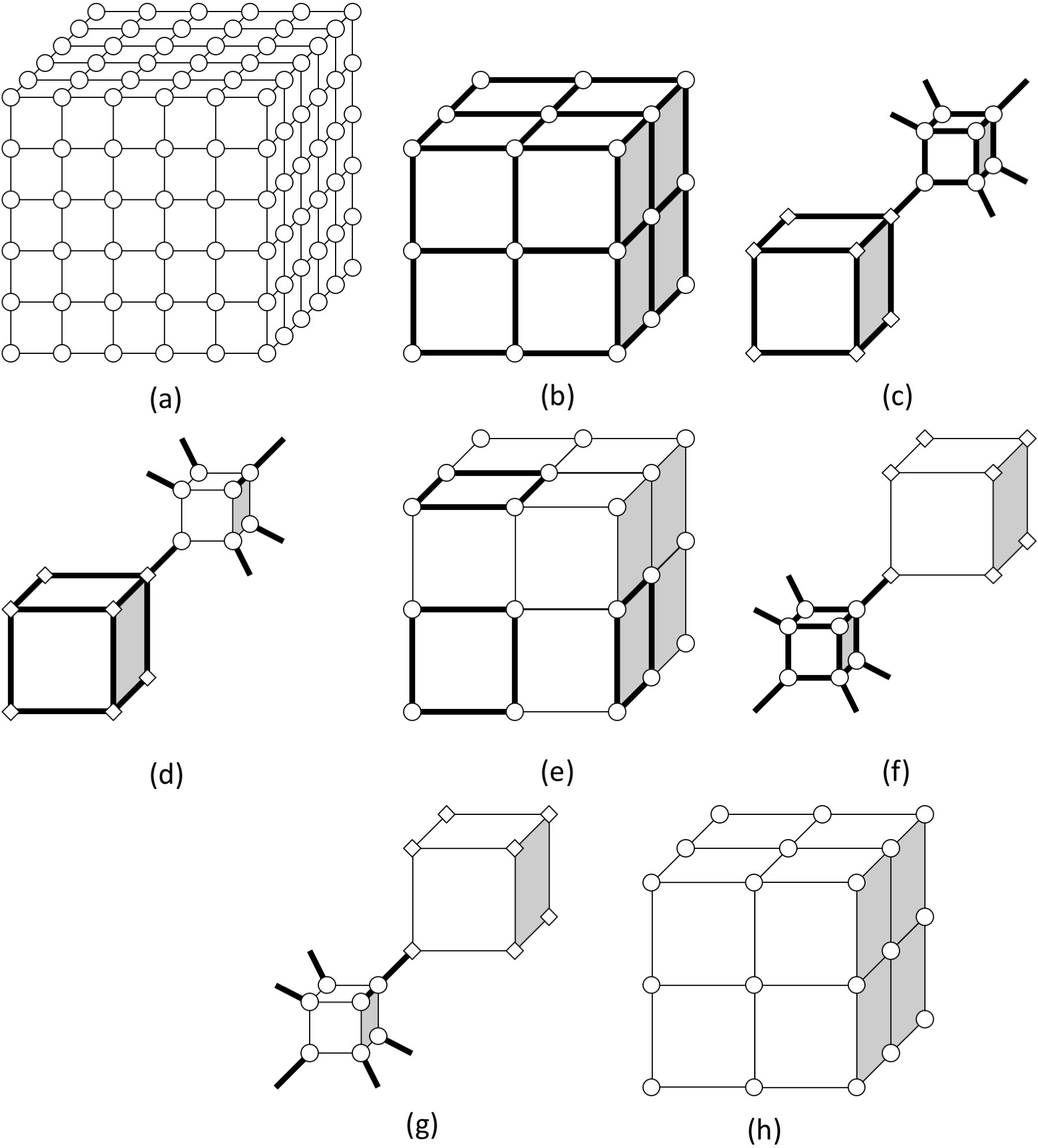
Figure 10. A single iteration of the tensor network skeletonization algorithm. The starting point is a tensor network with bond dimension $\chi$ and short-range correlation removed in $(0,0,0)_{2}$ and $(1,1,1)_{2}$ cubes. The final point is a coarse-grained tensor-network with 1/8 vertices (tensors). This coarse-grained tensor also has bond dimensions equal to $\chi$ and has short-range correlation removed for the (larger) $(0,0,0)_{2}$ and $(1,1,1)_{2}$ cubes.

The TNS algorithm consists of a sequence of coarse-graining iterations. At the beginning of each iteration (except the $0$-th iteration), we require the following iteration invariance to hold:

• for each of the $(0,0,0)_{2}$ and $(1,1,1)_{2}$ cubes, the short-range correlation has already been eliminated.

At the beginning of the $\ell$-th iteration, one holds a tensor network $(V^{\ell},E^{\ell},\{T^{i}\}_{i\in V_{\ell}})$ at level $\ell$ with $(n/2^{\ell})\times(n/2^{\ell})\times(n/2^{\ell})$ vertices. The $\ell$-th iteration consists of the following steps.

1. Contract the tensors at the eight vertices of each $(0,0,0)_{2}$ cube into a single tensor (see Figure 10(b)). The $(1,1,1)_{2}$ cubes are stretched and this results a new tensor network that contains $1/8$ of the vertices. The tensors at the new vertices are identical and the bond dimension of the new edges are equal to $\chi^{4}$ (shown with bold lines in the figure). Similar to the 2D case, the short-range correlations at level $\ell$ does not survive to level $\ell+1$ due to the iteration invariance. However, there are short-range correlations for the cubes at level $\ell+1$. The key task is to remove some of these short-range correlations and reduce the bond dimension back to $\chi$.

2. At each vertex $i$ in Figure 10(b), denote the tensor by $T^{i}_{abcdef}$ where $a$, $b$, $c$, $d$, $e$, and $f$ are the left, right, bottom, top, front, and back edges, respectively. By invoking three $UU^{\prime}T$-projection step (one for each of the left, bottom, and front edges), one effectively inserts two orthogonal (diamond) matrices in each of these edges. At each vertex $i$, further merge the tensor $T^{i}_{abcdef}$ with the six adjacent orthogonal (diamond) matrices. This step does not change the topology of the tensor network but the $T^{i}$ tensor has been modified.

3. For each $(1,1,1)_{2}$ cube in Figure 10(b), apply the $UR$-projection to the 6-tensor at each of its corners. Here the three edges adjacent to the cube are grouped together. Notice that the round $R$ tensors are placed close to the $(1,1,1)_{2}$ cube. This projection step only keeps the top $\chi^{3}$ singular values, i.e., the bond dimension of the diagonal edges are equal to $\chi^{3}$. The resulting graph is given in Figure 10(c).

4. In this key step, apply structure-preserving skeletonization to each of the $(1,1,1)_{2}$ cubes. The details of this procedure will be provided in Section 4.1.2. The resulting $(1,1,1)_{2}$ plaquette has short-range correlation removed and the bond dimensions of its 12 surrounding edges are reduced from $\chi^{4}$ to $\chi$ (see Figure 10(d)). One then merges back the $UR$-projections at its eight corners. The resulting tensor network in Figure 10(e) is similar to the one in Figure 10(b) but the short-range correlations in the $(1,1,1)_{2}$ plaquettes are now removed.

5. Now repeat the previous two steps to the $(0,0,0)_{2}$ plaquettes. This is illustrated in Figure 10(f), (g) and (h). The resulting tensor network has short-range correlation removed in both $(0,0,0)_{2}$ and $(1,1,1)_{2}$ plaquettes and the bond dimension of the edges is reduced back to $\chi$ from $\chi^{4}$.

This finishes the $\ell$-th iteration. At this point, one obtains a new tensor network denoted by $(V^{\ell+1},E^{\ell+1},\{T^{i}\}_{i\in V_{\ell+1}})$ that is a self-similar and coarse-grained version of $(V^{\ell},E^{\ell},\{T^{i}\}_{i\in V_{\ell}})$. This network satisfies the iteration invariance and can serve as the starting point of the next. iteration of the algorithm.

The last tensor network $(V^{L},E^{L},\{T^{i}\}_{i\in V_{L}})$ contains only a single $6$-tensor with the left and right edges identified and similarly for the bottom/top edges and front/back edges. Contracting this final tensor gives an approximation for the partition function. Similar to the 2D case, one can also introduce a modified version of this algorithm by removing short-range correlation for the $(1,1,1)_{2}$ cubes.

4.1.2. Structure-Preserving skeletonization

The structure-preserving skeletonization procedure for the 3D cubes is similar to the one introduced for 2D plaquette in Section 3.1.2. This procedure is illustrated in Figure 11 with the eight corner 4-tensors denoted by $P^{000}$, $P^{100}$, $P^{010}$, $P^{110}$, $P^{001}$, $P^{101}$, $P^{011}$, and $P^{111}$.

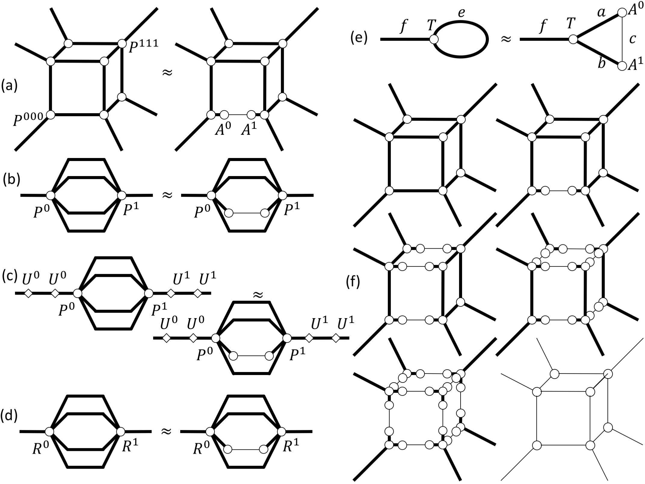
Figure 11. The structure-preserving skeletonization removes the short-range correlation within a $(1,1,1)_{2}$ or $(0,0,0)_{2}$ cube.

Instead of replacing the eight corner 4-tensors of the gray cube simultaneously, this procedure considers the 12 interior edges one by one and inserts within each edge two tensors of size $\chi^{4}\times\chi$.

1. Starting from the bottom front edge, the procedure seeks two 2-tensors $A^{0}$ and $A^{1}$ of size $\chi^{4}\times\chi$ with the condition that the 8-tensor of the new $(1,1,1)_{2}$ cube after the insertion approximates the original 8-tensors (see Figure 11(a)).

2. Merge the two left tensors $P^{000}$, $P^{001}$, $P^{010}$, and $P^{011}$ into a 5-tensor $P^{0}$ and merge the four right tensors into a 5-tensor $P^{1}$. After that, the condition is equivalent to the one given in Figure 11(b) with the two boundary edges have bond dimension equal to $(\chi^{3})^{4}=\chi^{12}$.

3. Since the bond dimensions of the two edges between $P^{0}$ and $P^{1}$ are to be reduced to $\chi$, this implies that the bond dimensions of the two boundary edges can be reduced to $\chi^{4}$ instead of $\chi^{12}$. As a result, one can perform the $UU^{\prime}T$-projection to both $P^{0}$ and $P^{1}$. This gives rise the condition in Figure 11(c).

4. Remove the two tensors $U^{0}$ and $U^{1}$ at the two endpoints, contract $U^{0}$ with $P^{0}$ to get a 3-tensor $R^{0}$, and contract $U^{1}$ with $P^{1}$ to get $R^{1}$. The approximation condition can now be written in terms of $R^{0}$ and $R^{1}$ as in Figure 11(d).

5. Finally, contracting the three other edge between $R^{0}$ and $R^{1}$ results a new 3-tensor $T$. The approximation condition now takes the form given in Figure 11(e). This is now exactly the setting of the skeletonization procedure and can be solved using the alternating least square algorithm proposed in Section 2.2.

At this point, two tensors $A^{0}$ and $A^{1}$ are successfully inserted into the bottom front edge. One can repeat this process also for the other three edges in the $x$ direction. Once this is done, we repeat this for the edges in the $y$ direction and then for the edges in the $z$ direction. At this point, there are in total 24 orthogonal tensors inserted in the 12 surrounding edges of the cube. Finally, merging each of the corner tensors with its three adjacent tensors gives the desired approximation (see Figure 11(f) for the whole process).

4.1.3. Numerical results

The critical temperature of the 3D statistical Ising model is $T_{c}\approx 4.5115$ but the free energy per site is not known explicitly. For a 3D periodic Ising model on a $2^{6}\times 2^{6}$ lattice, Figure 12 shows the free energy per site obtained through TNS for $\chi=2$ at different temperatures near the $T_{c}$. The obtained values of the free energy is close to the results obtained from other calculations using HOTRG or Monte Carlo calculations.

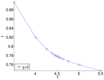
Figure 12. The free energy per site obtained through TNS at temperatures around $T_{c}$ for $\chi=2$ for the 3D periodic statistical Ising model.

4.2. Extensions

Similar to the 2D case, the 3D algorithm can be used to compute the average magnetization and the internal energy per site. When representing these quantities through tensor networks, one finds that only the 8 tensors at the center of the computational domain are different from the ones used in the partition function calculation. Therefore, the impurity tensor method can be applied as expected and the extra computational cost grows like $O(\log N)$ for any fixed $\chi$.

For disordered systems, the same discussion for the 2D systems applies. For example, for computing the order parameter of the 3D Edwards-Anderson model, one only needs to perform one impurity tensor computation for each site and thus the overall complexity grows like $O(N\log N)$ for any fixed $\chi$.

5. Ground state for quantum Ising models

In this section, we briefly touch on how to use TNS to efficiently represent the ground state of quantum many body system with periodic boundary condition. Consider for example a 1D periodic quantum Ising model. One can represent the ground state up to a constant factor using the Euclidean path integrals [Evenbly2015C]. After some preliminary tensor manipulations, this turns into a tensor network that is periodic in the spatial dimension and semi-infinite in the imaginary time dimension (see Figure 13(a)).

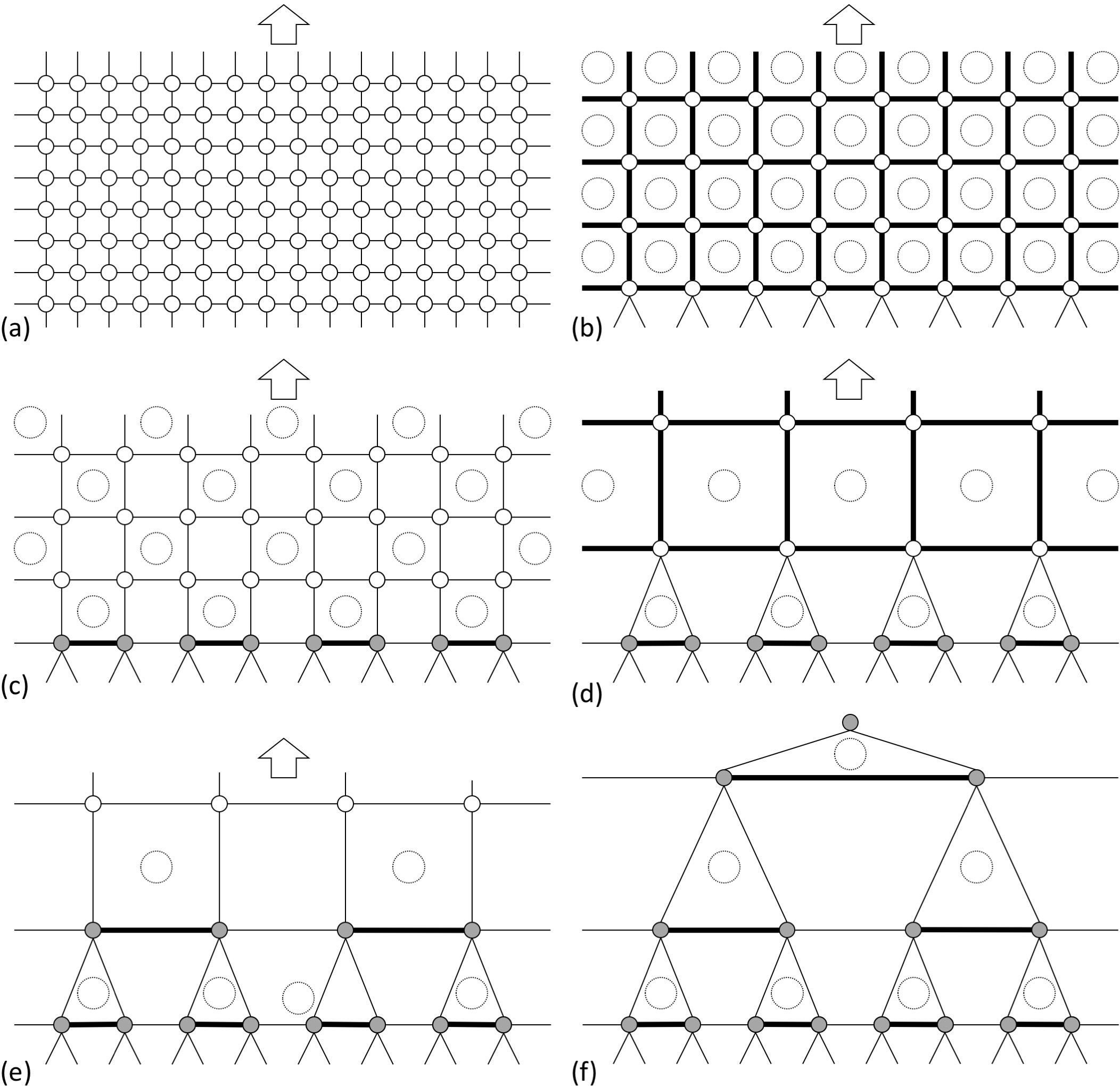
Figure 13. When applied to a Euclidean path integral formulation, TNS yields a new representation of the ground state of 1D quantum Ising model.

In the same fashion that the tensor network renormalization (TNR) gives rise to the multi-scale entanglement renormalization ansatz (MERA) [Evenbly2015B] for the ground state, TNS generates a new representation of the ground state as well. Illustrated in Figure 13, this process consists of the following steps.

1. First, contract each group of $2\times 2$ tensors (see Figure 13(b)). The new edges marked with bold lines have bond dimension equal to $\chi^{2}$.

2. Perform the structure-preserving skeletonization to all $(0,0)_{2}$ and $(1,1)_{2}$ plaquettes to remove the short-range correlations and reduce the bond dimension back to $\chi$. Notice that, after the structure-preserving skeletonization, the resulting tensors at the bottom level are different from the ones above due to their adjacency to the boundary. These special bottom level tensors are marked in gray (see Figure 13(c)).

3. Repeat this process to the remaining tensors above the bottom level. Contracting each group of $2\times 2$ tensors results a tensor network illustrated in Figure 13(d) and Figure 13(e).

4. One can repeat this process until reaching a half-infinite string of identical matrices. By extracting its top eigenvector, one can reduce this (up to a constant factor) to a 1-tensor at the top (see Figure 13(f)).

The final product is a hierarchical structure shown in Figure 13(f)). Though somewhat different from MERA, this new structure also has the capability of representing strongly entangled 1D quantum systems.

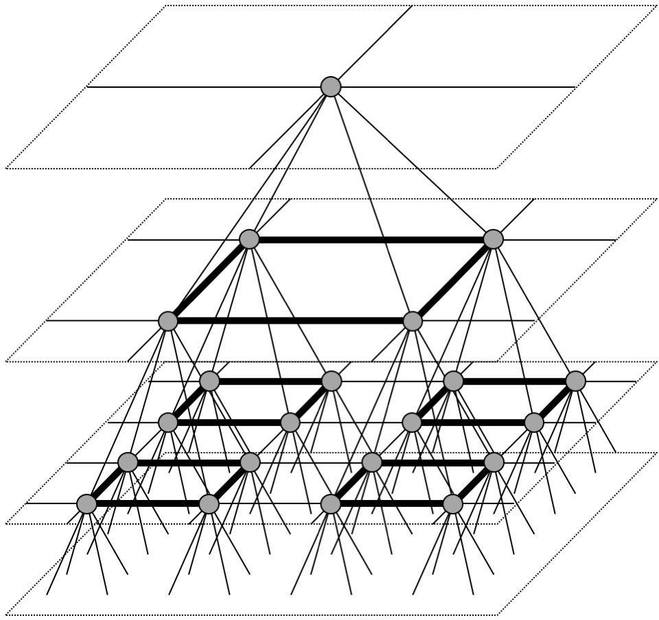
Figure 14. When applied to a Euclidean path integral formulation, TNS yields a new representation of the ground state of 2D quantum Ising model.

For 2D periodic quantum Ising model, the ground state can be represented via Euclidean path integral with a 3D tensor network which is periodic in the $x$ and $y$ directions but semi-infinite in the imaginary time direction. The above algorithm (with necessary modifications for the 3D TNS) can be applied to this tensor network and the result is a hierarchical structure (shown in Figure 14) that is capable of representing the ground state of strongly entangled 2D quantum systems effectively.

6. Conclusion

This paper introduced the tensor network skeletonization (TNS) as a new coarse-graining process for the numerical computation of tensor networks. At the heart of TNS is a new structure-preserving skeletonization procedure that removes short-range correlation effectively.

As to future work, an immediate task is to investigate other algorithms for the structure-preserving skeletonization problem (4) and (5). The alternating least square algorithm adopted here works quite well in practice. However, it would be interesting to understand why and also to consider other alternatives without using the somewhat artificial regularization parameter.

Most TNS algorithms introduced here are presented in their simplest forms in order to illustrate the main ideas. This means that they are not necessarily the most efficient implementations in practice. For example in the TNS algorithm for partition functions, one performs the contractions over all directions first and then applies the $UU^{\prime}T$-projections to these directions. However in practice, it is much more efficient to iterate over the directions and, for each direction, apply a $UU^{\prime}T$-projection right after the contraction of this direction.

We also plan to improve on the current implementations for the disordered systems and the ground state computations as well.