Two-dimensional light-front $\phi^{4}$ theory
in a symmetric polynomial basis

Abstract

We study the lowest-mass eigenstates of $\phi^{4}_{1+1}$ theory with both odd and even numbers of constituents. The calculation is carried out as a diagonalization of the light-front Hamiltonian in a Fock-space representation. In each Fock sector a fully symmetric polynomial basis is used to represent the Fock wave function. Convergence is investigated with respect to the number of basis polynomials in each sector and with respect to the number of sectors. The dependence of the spectrum on the coupling strength is used to estimate the critical coupling for the positive-mass-squared case. An apparent discrepancy with equal-time calculations of the critical coupling is resolved by an appropriate mass renormalization.

I Introduction

Although two-dimensional $\phi^{4}$ theory has a simple Lagrangian, the spectrum of the theory has some very interesting behavior. Even without the introduction of a negative bare-mass squared, the theory exhibits symmetry breaking at sufficiently strong coupling Chang , signaled by a degeneracy of the lowest massive states with the vacuum. Here we consider a light-front Hamiltonian calculation of the spectrum at and below this critical coupling and compare with previous calculations in both light-front VaryHari and equal-time quantization RychkovVitale ; LeeSalwen ; Sugihara ; SchaichLoinaz ; Bosetti ; Milsted . In particular, we explain why the two quantizations yield different results for the critical value of the bare dimensionless coupling.

Light-front quantization DLCQreview is in general a convenient approach to the nonperturbative solution of quantum field theories Vary ; ArbGauge , and provides an alternative to lattice Lattice and Dyson–Schwinger methods DSE . Light-front coordinates Dirac offer a clean separation between external and internal momenta, and the quantization can keep the vacuum trivial, so that it does not mix with the massive states. The wave functions of a Fock-state expansion are then well defined and lay an intuitive foundation for calculation of observables directly in terms of matrix elements of operators. Moreover, the formulation is in Minkowski space rather than the Euclidean space of lattice gauge theory and Dyson–Schwinger equations.

In two dimensions, light-front quantization uses a time coordinate $x^{+}\equiv t+z$ and a spatial coordinate $x^{-}\equiv t-z$. The conjugate momentum variables are $p^{-}\equiv E-p_{z}$ and $p^{+}\equiv E+p_{z}$, respectively. The fundamental eigenvalue problem for an eigenstate of mass $M$ is ${\cal P}^{-}|\psi(P^{+})\rangle=\frac{M^{2}}{P^{+}}|\psi(P^{+})\rangle$, where ${\cal P}^{-}$ is the light-front Hamiltonian and $P^{+}$ is the total light-front momentum of the state. We solve this eigenvalue problem by expanding $|\psi(P^{+})\rangle$ in a Fock basis of momentum and particle-number eigenstates and then expanding the Fock-space wave functions in terms of fully symmetric, multivariate polynomials GenSymPolys . The problem is made finite by truncation in both the Fock-space and polynomial basis sets.

The use of a polynomial basis for the wave functions has significant advantages over the more common discretized light-cone quantization (DLCQ) approach PauliBrodsky ; DLCQreview . One purpose of the present work is to illustrate this. In DLCQ, which relies on a trapezoidal approximation to integral operators, endpoint corrections associated with zero modes ZeroModes are normally dropped, which delays convergence, whereas a basis-function method can be tuned to keep the correct endpoint behavior of the wave functions. Also, the discretization grid of DLCQ forces a particular allocation of computational resources to each Fock sector, without regard to the importance of one sector over another; a basis-function approach allows the allocation to be adjusted sector by sector, to optimize computation resources with respect to convergence. The particular polynomial basis that we use GenSymPolys is specifically symmetric with respect to interchange of the identical bosons, so that no explicit symmetrization is required.

The remainder of the paper is structured as follows. Section II describes the eigenvalue problem that we solve, with details of the coupled integral equations for the Fock-state wave functions. In Sec. III we discuss the difference in mass renormalizations for light-front and equal-time quantization and provide a scheme for calculation. Our results are presented and discussed in Sec. IV, with a brief summary provided in Sec. V. Details of the numerical calculation are given in an Appendix.

II Light-front eigenvalue problem

From the Lagrangian for two-dimensional $\phi^{4}$ theory

$${\cal L}=\frac{1}{2}(\partial_{\mu}\phi)^{2}-\frac{1}{2}\mu^{2}\phi^{2}-\frac{\lambda}{4!}\phi^{4},$$ (1)

where $\mu$ is the mass of the boson and $\lambda$ is the coupling constant, the light-front Hamiltonian density is found to be

$${\cal H}=\frac{1}{2}\mu^{2}\phi^{2}+\frac{\lambda}{4!}\phi^{4}.$$ (2)

The mode expansion for the field at zero light-front time is

$$\phi(x^{+}=0,x^{-})=\int\frac{dp}{\sqrt{4\pi p}}\left\{a(p)e^{-ipx^{-}/2}+a^{\dagger}(p)e^{ipx^{-}/2}\right\},$$ (3)

where for convenience we have dropped the $+$ superscript and will from here on write light-front momenta such as $p^{+}$ as just $p$. The creation operator $a^{\dagger}(p)$ satisfies the commutation relation

$$[a(p),a^{\dagger}(p^{\prime})]=\delta(p-p^{\prime}),$$ (4)

and builds $m$-constituent Fock states from the Fock vacuum $|0\rangle$ in the form

$$|y_{i}P;P,m\rangle=\frac{1}{\sqrt{m!}}\prod_{i=1}^{m}a^{\dagger}(y_{i}P)|0\rangle.$$ (5)

Here $y_{i}\equiv p_{i}/P$ is the longitudinal momentum fraction for the $i$th constituent.

The light-front Hamiltonian is ${\cal P}^{-}={\cal P}^{-}_{11}+{\cal P}^{-}_{22}+{\cal P}^{-}_{13}+{\cal P}^{-}_{31}$, with

$${\cal P}^{-}_{11} = \int dp\frac{\mu^{2}}{p}a^{\dagger}(p)a(p),$$ (6)

$${\cal P}^{-}_{22} = \frac{\lambda}{4}\int\frac{dp_{1}dp_{2}}{4\pi\sqrt{p_{1}p_{2}}}\int\frac{dp^{\prime}_{1}dp^{\prime}_{2}}{\sqrt{p^{\prime}_{1}p^{\prime}_{2}}}\delta(p_{1}+p_{2}-p^{\prime}_{1}-p^{\prime}_{2})$$

$$\rule{144.54pt}{0.0pt}\times a^{\dagger}(p_{1})a^{\dagger}(p_{2})a(p^{\prime}_{1})a(p^{\prime}_{2}),$$

$${\cal P}^{-}_{13} = \frac{\lambda}{6}\int\frac{dp_{1}dp_{2}dp_{3}}{4\pi\sqrt{p_{1}p_{2}p_{3}(p_{1}+p_{2}+p_{3})}}a^{\dagger}(p_{1}+p_{2}+p_{3})a(p_{1})a(p_{2})a(p_{3}),$$ (8)

$${\cal P}^{-}_{31} = \frac{\lambda}{6}\int\frac{dp_{1}dp_{2}dp_{3}}{4\pi\sqrt{p_{1}p_{2}p_{3}(p_{1}+p_{2}+p_{3})}}a^{\dagger}(p_{1})a^{\dagger}(p_{2})a^{\dagger}(p_{3})a(p_{1}+p_{2}+p_{3}).$$ (9)

The subscripts indicate the number of creation and annihilation operators in each term.

The Fock-state expansion of an eigenstate can be written

$$|\psi(P)\rangle=\sum_{m}P^{\frac{m-1}{2}}\int\prod_{i}^{m}dy_{i}\delta(1-\sum_{i}^{m}y_{i})\psi_{m}(y_{i})|y_{i}P;P,m\rangle,$$ (10)

where $\psi_{m}$ is the wave function for $m$ constituents. Because the terms of ${\cal P}^{-}$ change particle number by zero or by two, the eigenstates can be separated according to the oddness or evenness of the number of constituents. Therefore, the first sum in (10) is restricted to odd or even $m$. We will consider only the lowest mass eigenstate in each case, though the methods allow for calculation of higher states.

The light-front Hamiltonian eigenvalue problem ${\cal P}^{-}|\psi(P)\rangle=\frac{M^{2}}{P}|\psi(P)\rangle$ reduces to a coupled set of integral equations for the Fock-state wave functions:

$$m\frac{\mu^{2}}{y_{1}P}\psi_{m}(y_{i})+\frac{\lambda}{4\pi P}\frac{m(m-1)}{4\sqrt{y_{1}y_{2}}}\int\frac{dx_{1}dx_{2}}{\sqrt{x_{1}x_{2}}}\delta(y_{1}+y_{2}-x_{1}-x_{2})\psi_{m}(x_{1},x_{2},y_{3},\ldots,y_{m})$$ (11)

$$+\frac{\lambda}{4\pi P}\frac{m}{6}\sqrt{(m+2)(m+1)}\int\frac{dx_{1}dx_{2}dx_{3}}{\sqrt{y_{1}x_{1}x_{2}x_{3}}}\delta(y_{1}-x_{1}-x_{2}-x_{3})\psi_{m+2}(x_{1},x_{2},x_{3},y_{2},\ldots,y_{m})$$

$$+\frac{\lambda}{4\pi P}\frac{m-2}{6}\frac{\sqrt{m(m-1)}}{\sqrt{y_{1}y_{2}y_{3}(y_{1}+y_{2}+y_{3})}}\psi_{m-2}(y_{1}+y_{2}+y_{3},y_{4},\ldots,y_{m})=\frac{M^{2}}{P}\psi_{m}(y_{i}).$$

We have used the symmetry of $\psi_{m}$ to collect exchanged momenta in the leading arguments of the function, with appropriate $m$-dependent factors in front of each term. The equations are simplified further by the introduction of a dimensionless coupling

$$g\equiv\frac{\lambda}{4\pi\mu^{2}}$$ (12)

and by multiplying the set by $P/\mu^{2}$, to obtain

$$\frac{m}{y_{1}}\psi_{m}(y_{i})+\frac{g}{4}\frac{m(m-1)}{\sqrt{y_{1}y_{2}}}\int\frac{dx_{1}dx_{2}}{\sqrt{x_{1}x_{2}}}\delta(y_{1}+y_{2}-x_{1}-x_{2})\psi_{m}(x_{1},x_{2},y_{3},\ldots,y_{m})$$ (13)

$$+\frac{g}{6}m\sqrt{(m+2)(m+1)}\int\frac{dx_{1}dx_{2}dx_{3}}{\sqrt{y_{1}x_{1}x_{2}x_{3}}}\delta(y_{1}-x_{1}-x_{2}-x_{3})\psi_{m+2}(x_{1},x_{2},x_{3},y_{2},\ldots,y_{m})$$

$$+\frac{g}{6}\frac{(m-2)\sqrt{m(m-1)}}{\sqrt{y_{1}y_{2}y_{3}(y_{1}+y_{2}+y_{3})}}\psi_{m-2}(y_{1}+y_{2}+y_{3},y_{4},\ldots,y_{m})=\frac{M^{2}}{\mu^{2}}\psi_{m}(y_{i}).$$

It is this set of equations that we solve numerically, as described in the Appendix. Our approach takes advantage of the new set of multivariate polynomials that is fully symmetric on the hypersurface $\sum_{i}y_{i}=1$ defined by momentum conservation GenSymPolys . This allows independent tuning of resolutions in each Fock sector, so that, unlike discrete light-cone quantization (DLCQ) PauliBrodsky ; DLCQreview , sectors with lower net probability need not overtax computational resources. Also, within each Fock sector, the use of a polynomial basis has improved convergence compared to DLCQ GenSymPolys , at least partly because DLCQ misses contributions from zero modes ZeroModes associated with integrable singularities at $y_{i}=0$.

In addition to calculation of the spectrum, it is possible to calculate the expectation value for the field $\phi$ when the odd and even states are degenerate. At degeneracy, the two states mix, and the expectation value for $\phi$ comes from cross terms, the matrix element between the odd and even eigenstates. Let $|\widetilde{\psi}(P^{\prime})\rangle$ be the state with an odd number of constituents, and $|\psi(P)\rangle$ be the state for an even number. At degeneracy, the eigenstate can be a linear combination of these, and the desired matrix element for the field is

$$\langle\widetilde{\psi}(P^{\prime})|\phi(0,x^{-})|\psi(P)\rangle=\sum_{m}\frac{P^{\prime\,m/2-1}}{P^{(m-1)/2}}\int\prod_{j}^{m+1}dy^{\prime}_{j}\delta(1-\sum_{j}y^{\prime}_{j})\frac{\sqrt{m+1}}{\sqrt{4\pi y^{\prime}_{1}P^{\prime}}}$$

$$\rule{72.26999pt}{0.0pt}\times\delta(y^{\prime}_{1}+P/P^{\prime}-1)e^{i(P^{\prime}-P)x^{-}/2}\widetilde{\psi}_{m+1}(y^{\prime}_{j})\psi_{m}(y^{\prime}_{2},...,y^{\prime}_{m+1})$$

$$\rule{36.135pt}{0.0pt}+\sum_{m}\frac{P^{m/2-1}}{P^{\prime\,(m-1)/2}}\int\prod_{j}^{m+1}dy_{j}\delta(1-\sum_{j}y_{j})\frac{\sqrt{m+1}}{\sqrt{4\pi y_{1}P}}\delta(y_{1}+P^{\prime}/P-1)$$

$$\rule{72.26999pt}{0.0pt}\times e^{-i(P^{\prime}-P)x^{-}/2}\widetilde{\psi}_{m}(y_{2},\ldots,y_{m+1})\psi_{m+1}(y_{j}),$$

where again we have taken advantage of the wave-function symmetry to arrange for all but the first constituent to be spectators. In the limit $P^{\prime}\rightarrow P$, this expression reduces to

$$\langle\widetilde{\psi}(P)|\phi(0,x^{-})|\psi(P)\rangle=\frac{1}{2}\sum_{m}\frac{\sqrt{m+1}}{\sqrt{4\pi P}}\int\prod_{i=2}^{m+1}dy_{i}\delta(1-\sum_{i}y_{i})$$

$$\rule{36.135pt}{0.0pt}\times\left[\widetilde{\phi}_{m+1}(y_{2},\ldots,y_{m+1})\psi_{m}(y_{2},\ldots,y_{m+1})+\widetilde{\psi}_{m}(y_{2},\ldots,y_{m+1})\phi_{m+1}(y_{2},\ldots,y_{m+1})\right],$$

with

$$\phi_{m+1}(y_{2},\ldots,y_{m+1})\equiv\lim_{y_{1}\rightarrow 0}\frac{1}{\sqrt{y_{1}}}\psi_{m+1}(y_{1},y_{2},\ldots,y_{m})$$ (16)

and $\widetilde{\phi}$ defined analogously. Thus the expectation value depends upon zero modes ZeroModes . In our basis function approach, the zero-momentum limit can be taken explicitly.

III Mass renormalization

One of the advantages of light-front quantization is the absence of vacuum-to-vacuum graphs DLCQreview . However, to compare results found in equal-time quantization at equivalent values of the bare parameters in the Lagrangian, this absence must be taken into account. In particular, the bare mass in $\phi^{4}_{1+1}$ theory is renormalized by tadpole contributions in equal-time quantization but not in light-front quantization, and the two different masses are related by SineGordon

$$\mu_{\rm LF}^{2}=\mu_{\rm ET}^{2}+\lambda\left[\langle 0|:\frac{\phi^{2}}{2}:|0\rangle-\langle 0|:\frac{\phi^{2}}{2}:|0\rangle_{\rm free}\right].$$ (17)

The vacuum expectation values (vev) of $\phi^{2}$ resum the tadpole contributions; the subscript free indicates the vev with $\lambda=0$. This distinction between bare masses in the two quantizations implies that the dimensionless coupling $g=\lambda/4\pi\mu^{2}$ is also not the same. Estimates of the critical coupling must then be adjusted for the difference if they are to be compared.

Of course, if one compares results only for physical quantities, the two quantizations should match immediately. However, this is not straightforward in the case of the critical coupling, where the physical mass scale goes to zero.

With the tadpole contribution re-expressed as a vev, we can calculate the contribution in light-front quantization and avoid doing a second, equal-time calculation. The vev is regulated by point splitting, and a sum over a complete set states is introduced, to obtain

$$\langle 0|:\frac{\phi^{2}}{2}:|0\rangle\rightarrow\frac{1}{2}\langle 0|\phi(\epsilon^{+},\epsilon^{-})\int_{0}^{\infty}dP\sum_{n}|\psi_{n}(P)\rangle\langle\psi_{n}(P)|\phi(0,0)|0\rangle.$$ (18)

Each mass eigenstate $|\psi_{n}(P)\rangle$ is expanded in terms of Fock states and wave functions, just as in (10), with the Fock wave functions $\psi_{nm}(y_{i})$ now defined with an additional index $n$ for the particular eigenstate. Because the $\phi$ field changes particle number by one, only one-particle Fock states will contribute to the sum over $n$, with amplitude $\psi_{n1}$. For the free case, the only contribution to the sum is the one-particle state $a^{\dagger}(P)|0\rangle$.

The individual matrix elements are readily calculated. At $x^{+}=0$ the field is given by (3), and the matrix element is

$$\langle\psi_{n}(P)|\phi(0,0)|0\rangle=\langle 0|\psi_{n1}^{*}a(P)\int\frac{dp}{\sqrt{4\pi p}}a^{\dagger}(p)|0\rangle=\frac{\psi_{n1}^{*}}{\sqrt{4\pi P}}$$ (19)

At $x^{+}=\epsilon^{+}$, the field is

$$\phi(\epsilon^{+},\epsilon^{-})=e^{i{\cal P}^{-}\epsilon^{+}/2}\phi(0,\epsilon^{-})e^{-i{\cal P}^{-}\epsilon^{+}/2}.$$ (20)

The matrix element is

$$\langle 0|\phi(\epsilon^{+},\epsilon^{-})|\psi_{n}(P)\rangle = \langle 0|e^{i0\epsilon^{+}}\int\frac{dp}{\sqrt{4\pi p}}a(p)e^{-ip\epsilon^{-}/2}e^{-iM_{n}^{2}\epsilon^{+}/2P}\psi_{n1}a^{\dagger}(P)|0\rangle$$ (21)

$$= \frac{\psi_{n1}}{\sqrt{4\pi P}}e^{-i(P\epsilon^{-}+M_{n}^{2}\epsilon^{+}/P)/2},$$

with $M_{n}$ the mass of the $n$th state. The corresponding matrix elements for the free case are

$$\langle 0|a(P)\phi(0,0)|0\rangle=\langle 0|a(P)\int\frac{dp}{\sqrt{4\pi p}}a^{\dagger}(p)|0\rangle=\frac{1}{\sqrt{4\pi P}}$$ (22)

and

$$\langle 0|\phi(\epsilon^{+},\epsilon^{-})a^{\dagger}(P)|0\rangle = \langle 0|e^{i0\epsilon^{+}}\int\frac{dp}{\sqrt{4\pi p}}a(p)e^{-ip\epsilon^{-}/2}e^{-i\mu^{2}\epsilon^{+}/2P}a^{\dagger}(P)|0\rangle$$ (23)

$$= \frac{1}{\sqrt{4\pi P}}e^{-i(P\epsilon^{-}+\mu^{2}\epsilon^{+}/P)/2}.$$

The combination of these matrix elements yields the two vev’s:

$$\langle 0|:\frac{\phi^{2}}{2}:|0\rangle=\frac{1}{2}\sum_{n}\int_{0}^{\infty}dP\frac{|\psi_{n1}|^{2}}{4\pi P}e^{-i(P\epsilon^{-}+M_{n}^{2}\epsilon^{+}/P)/2}$$ (24)

and

$$\langle 0|:\frac{\phi^{2}}{2}:|0\rangle_{\rm free}=\frac{1}{2}\int_{0}^{\infty}dP\frac{1}{4\pi P}e^{-i(P\epsilon^{-}+\mu^{2}\epsilon^{+}/P)/2}.$$ (25)

The completeness of the eigenstates allows the introduction of the sum $1=\sum_{n}|\psi_{n1}|^{2}$ into the free vev, so that the difference can be written

$$\langle 0|:\frac{\phi^{2}}{2}:|0\rangle-\langle 0|:\frac{\phi^{2}}{2}:|0\rangle_{\rm free}=\sum_{n}\frac{|\psi_{n1}|^{2}}{8\pi}\int_{0}^{\infty}\frac{dP}{P}e^{-iP\epsilon^{-}/2}\left[e^{-i\frac{M_{n}^{2}\epsilon^{+}}{2P}}-e^{-i\frac{\mu^{2}\epsilon^{+}}{2P}}\right].$$ (26)

With the change of variable $P=2z\epsilon^{+}$ and the introduction of a convergence factor $e^{-\eta z}$, this expression becomes

$$\langle 0|:\frac{\phi^{2}}{2}:|0\rangle-\langle 0|:\frac{\phi^{2}}{2}:|0\rangle_{\rm free}=\sum_{n}\frac{|\psi_{n1}|^{2}}{8\pi}\int_{0}^{\infty}\frac{dz}{z}e^{iz(-\epsilon^{2}+i\eta)}\left[e^{-i\frac{M_{n}^{2}}{4z}}-e^{-i\frac{\mu^{2}}{4z}}\right].$$ (27)

Each term is an integral representation GradshteynRyzhik of the modified Bessel function $K_{0}$:

$$\int_{0}^{\infty}\frac{dx}{x}\exp\left(i\frac{\alpha}{2}\left[x-\frac{\beta^{2}}{x}\right]\right)=2K_{0}(\alpha\beta),$$ (28)

with positive imaginary parts for $\alpha$ and $\alpha\beta^{2}$. The difference of vev’s then becomes

$$\langle 0|:\frac{\phi^{2}}{2}:|0\rangle-\langle 0|:\frac{\phi^{2}}{2}:|0\rangle_{\rm free}=\sum_{n}\frac{|\psi_{n1}|^{2}}{4\pi}\left[K_{0}(M_{n}\sqrt{-\epsilon^{2}+i\eta})-K_{0}(\mu\sqrt{-\epsilon^{2}+i\eta})\right].$$ (29)

As $-\epsilon^{2}+i\eta$ goes to zero, the only contribution from $K_{0}$ is a simple logarithm, i.e. $K_{0}(z)\rightarrow-\ln(z/2)-\gamma$, leaving

$$\langle 0|:\frac{\phi^{2}}{2}:|0\rangle-\langle 0|:\frac{\phi^{2}}{2}:|0\rangle_{\rm free}=-\sum_{n}\frac{|\psi_{n1}|^{2}}{4\pi}\ln\frac{M_{n}}{\mu_{\rm LF}}\equiv-\Delta/4\pi,$$ (30)

with $\mu$ written as $\mu_{\rm LF}$ to emphasize that it is the light-front bare mass. Within the context of our numerical calculation, the terms of the sum can be computed by fully diagonalizing the matrix representation of the Hamiltonian ${\cal P}^{-}$.

The bare masses in the two quantizations are then related by

$$\mu_{\rm LF}^{2}=\mu_{\rm ET}^{2}-\frac{\lambda}{4\pi}\Delta\;\;\mbox{or}\;\;\frac{\mu_{\rm ET}^{2}}{\mu_{\rm LF}^{2}}=1+g_{\rm LF}\Delta.$$ (31)

The bare-mass ratio is what connects the dimensionless couplings and masses obtained in the two quantizations:

$$g_{\rm ET}=\frac{g_{\rm LF}}{\mu_{\rm ET}^{2}/\mu_{\rm LF}^{2}}=\frac{g_{\rm LF}}{(1+g_{\rm LF}\Delta)}\;\;\mbox{and}\;\;\frac{M^{2}}{\mu_{\rm ET}^{2}}=\frac{M^{2}/\mu_{\rm LF}^{2}}{\mu_{\rm ET}^{2}/\mu_{\rm LF}^{2}}=\frac{1}{1+g_{\rm LF}\Delta}\frac{M^{2}}{\mu_{\rm LF}^{2}},$$ (32)

which we can use to compare the values obtained.

IV Results and discussion

With the numerical methods discussed in the Appendix, we have solved the eigenvalue problem for the lowest odd and even states. The mass values for different Fock-space truncations are shown in Figs. 1 and 2. The error bars are estimated based on the extrapolations in basis size. The seven/eight-body truncations yield results that are the same as the five/six-body results, to within the error estimates, which means that convergence in the Fock-state expansion has been achieved.

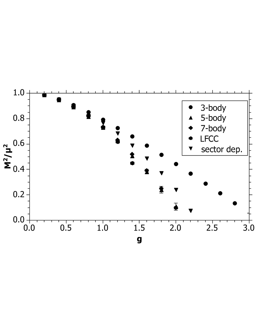
Figure 1: Lowest mass eigenvalue for odd numbers of constituents. Results are shown for different Fock-space truncations to three, five, and seven constituents. Also plotted are results for the leading light-front coupled-cluster (LFCC) approximation and for a sector-dependent modification of the three-body truncation. The errors are estimated from extrapolations in polynomial basis size.

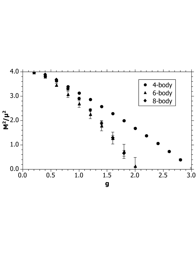
Figure 2: Same as Fig. 1 but for even numbers of constituents, with Fock-space truncations at four, six and eight.

In the odd case, we also show results from the leading light-front coupled-cluster (LFCC) approximation LFCC ; LFCCphi4 and a modification of the three-body truncation that includes sector-dependent bare masses Wilson ; hb ; Karmanov ; SecDep . The LFCC calculation includes a partial summation over all higher Fock states. The sector-dependent calculation uses the physical mass in the upper Fock sector, where there can be no self-energy correction. Both of these alternatives require solution of a three-body problem and yield results much better than the simple three-body truncation, with the LFCC approximation doing much better than the sector-dependent approach.

The relative Fock-sector probabilities for the odd case are plotted in Fig. 3. These ratios are computed as

$$R_{m}\equiv\frac{1}{|\psi_{1}|^{2}}\int\left[\prod_{i=1}^{m-1}dy_{i}\right]|\psi_{m}(y_{i})|^{2}=\frac{1}{|\psi_{1}|^{2}}\sum_{ni}|c_{ni}^{(m)}|^{2},$$ (33)

where the last expression is in terms of the basis-function expansion coefficients, as defined in (34). These ratios show that the probability for each Fock sector decreases by an order of magnitude when the number of constituents goes up by two.

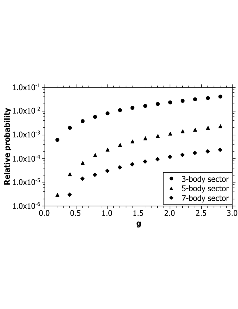
Figure 3: Relative Fock-sector probabilities for the lowest mass eigenstate with odd numbers of constituents.

The apparent convergence of the Fock-state expansion is somewhat deceptive. With the bare mass fixed as the same in all Fock sectors, the higher Fock sectors are suppressed by the large invariant mass of each Fock state, which is of order $m\mu$ for the sector with $m$ constituents. For weak to moderate couplings this is not a particular concern, but for strong coupling, approaching the critical value, one expects much larger contributions from higher Fock states. This would be best modeled by sector-dependent masses. However, to use sector-dependent masses requires renormalization to physical observables, which would greatly complicate any comparison with the published results for equal-time quantization. Therefore, for purposes of the the present work, we retain a fixed bare mass.

Based on the results for the masses as a function of the coupling, we can estimate a critical coupling as the value at which the lowest masses reach zero. This intersection is illustrated in Fig. 4, where the lowest mass-squared values are plotted as well as four times the odd-eigenstate mass squared. Because there are no bound states in this theory the lowest even-eigenstate mass should be equal to this; the difference in the plot is another measure of the numerical and truncation errors. From this plot, we estimate the critical value of the dimensionless coupling to be 2.1$\pm$0.05. For comparison, we list in Table 1 this and values from other computations, as gathered in RychkovVitale ; however, because the definitions of dimensionless couplings vary, the table uses the definition $\bar{g}\equiv\lambda/24\mu^{2}$, which is just $\frac{\pi}{6}g$.

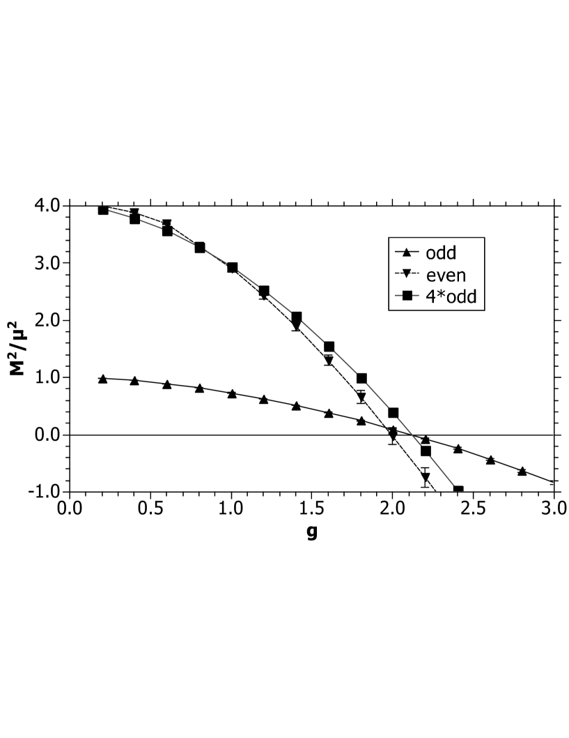
Figure 4: The lowest masses for the odd and even cases, as used to estimate the critical coupling, including a plot of the threshold for two-particle states at four times the mass-squared of the odd case.

Table 1: Comparison of critical coupling values, adapted from RychkovVitale , with a slightly different definition of the dimensionless coupling $\bar{g}=\frac{\pi}{6}g$. The first two values were computed in light-front quantization and the remainder in equal-time quantization; the results are comparable but only after the different mass renormalizations are taken into account, as discussed in the text.

Method	$\bar{g}_{c}$	Reported by
Light-front symmetric polynomials	$1.1\pm 0.03$	this work
DLCQ	1.38	Harindranath & Vary VaryHari
Quasi-sparse eigenvector	2.5	Lee & Salwen LeeSalwen
Density matrix renormalization group	2.4954(4)	Sugihara Sugihara
Lattice Monte Carlo	2.70$\left\{\begin{array}[]{l}+0.025\\ -0.013\end{array}\right.$	Schaich & Loinaz SchaichLoinaz
	$2.79\pm 0.02$	Bosetti et al. Bosetti
Uniform matrix product	2.766(5)	Milsted et al. Milsted
Renormalized Hamiltonian truncation	2.97(14)	Rychkov & Vitale RychkovVitale

The results listed in Table 1 imply a systematic difference between equal-time and light-front values for the critical coupling, which is exactly what should be expected, based on the difference in mass renormalizations discussed in Sec. III. To quantify this difference, we extended the diagonalization of the Hamiltonian matrix to include the entire spectrum and computed the shift $\Delta$, defined in (30). The results are plotted in Fig. 5, along with extrapolations of fits to the shifts for coupling values below 1.

Higher coupling values are not used in the fits because the lack of sector-dependent mass renormalization does not allow a reasonable approximation to the wave functions. The one-particle sector should become less and less probable for the lowest eigenstate, as the critical coupling is approached and as its mass approaches zero; instead, the one-particle probability remains finite and the product $|\psi_{11}|\ln(M_{1}^{2})$ diverges. To judge the value of the coupling where this effect becomes noticeable, we studied the behavior of the dimensionless mass $M^{2}/\mu_{\rm ET}^{2}$, as predicted by (32), as a function of the coupling, which we plot in Fig. 6. For coupling values above 1, the mass begins to increase rather than decrease; this incorrect behavior is the precursor of the divergence at the critical coupling; we also see that the convergence with respect to the polynomial basis becomes somewhat worse at these larger coupling values.

The estimated value of the shift at the critical coupling 2.1, based on the two extrapolations, is $\Delta(g=2.1)=-0.47\pm 0.12$. The value is from the higher-order extrapolation, with the lower-order extrapolation used to indicate the error. From the latest equal-time value for the critical coupling RychkovVitale , $g_{\rm ETc}=\frac{6}{\pi}2.97=5.67$, we extract a shift of $(g_{\rm LFc}/g_{\rm ETc}-1)/g_{\rm LFc}=-0.30$, which is consistent with the estimated value of the shift.

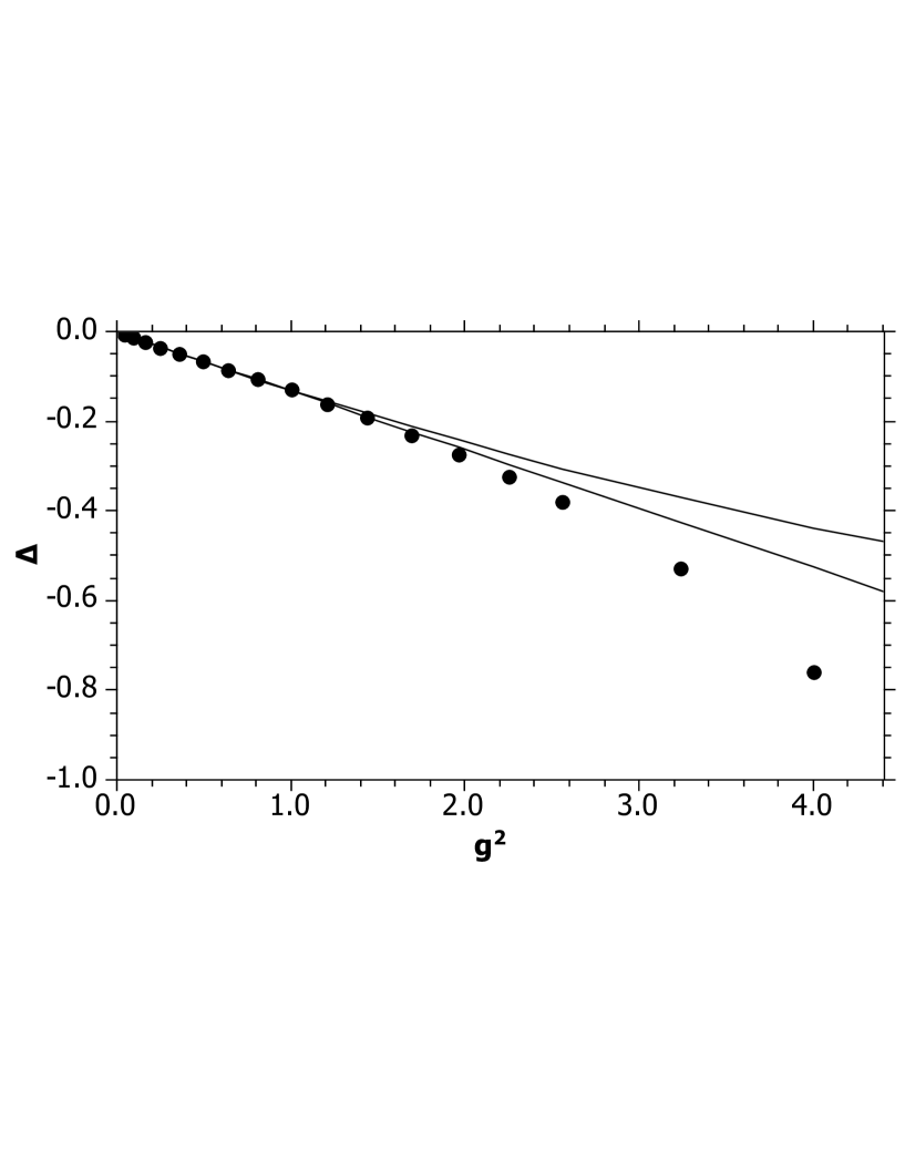
Figure 5: The renormalization shift $\Delta$, defined in Eq. (30) of the text, as a function of the square of the dimensionless coupling $g$. The points displayed are obtained as extrapolations in the polynomial basis size. The lines are linear and quadratic fits to shifts below $g=1$, extrapolated to the region of the critical coupling.

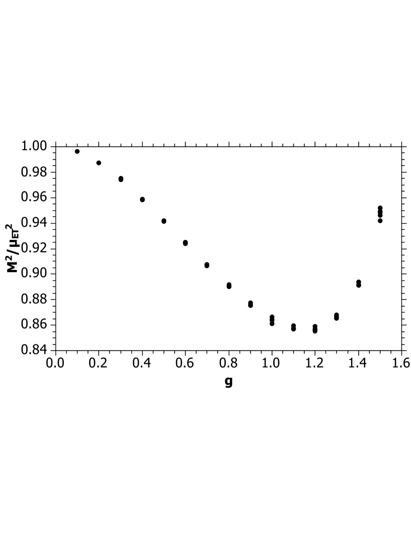
Figure 6: Lowest equal-time mass eigenvalues for odd numbers of constituents plotted versus the dimensionless light-front coupling $g$. Each mass value is obtained from the light-front masses and the computed shift $\Delta$ according to Eq. (32) of the text. Different points at the same $g$ value correspond to different truncations of the polynomial basis size.

V Summary

We have developed a high-order method for ($1+1$)-dimensional light-front theories that is distinct from DLCQ PauliBrodsky ; DLCQreview . It is based on fully symmetric multivariate polynomials GenSymPolys that respect the momentum conservation constraint and allows separate tuning of resolutions in each Fock sector. This method could be combined with transverse discretization or basis functions for numerical solution of ($3+1$)-dimensional theories.

As an illustration, the method has been applied here to $\phi^{4}_{1+1}$ theory. The lowest mass eigenvalues have been computed, as shown in Figs. 1 and 2; they converge rapidly with respect to the Fock-space truncation. The odd case includes comparison with the light-front coupled-cluster (LFCC) method LFCC ; LFCCphi4 , which indicates that the LFCC method combined with symmetric polynomials shows promise for rapid convergence. Either approach can also be applied to the negative-mass squared case, where the symmetry breaking is explicit.

From the behavior of the mass eigenstates with respect to coupling strength, as shown in Fig. 4, we have extracted an estimate of the critical coupling for $\phi^{4}_{1+1}$ theory with positive mass squared. Above this coupling, the symmetry is broken. With mass renormalization properly taken into account, as discussed in Sec. III, the value obtained ($g_{c}=2.1\pm 0.05$ or $\bar{g}_{c}=1.1\pm 0.03$) is comparable to values obtained in equal-time quantization.

The calculation can be improved by invocation of sector-dependent mass renormalization Wilson ; hb ; Karmanov ; SecDep , so that higher Fock states can make a significant contribution as the coupling approaches the critical value. However, any comparison with equal-time quantization will then require the use of physical quantities as reference points, rather than a direct comparison of bare couplings.

Appendix A Numerical methods

The coupled system of equations for the Fock-state wave functions are solved numerically using an expansion in terms of fully symmetric polynomials GenSymPolys . The coefficients of the expansion satisfy a matrix eigenvalue problem, which is then diagonalized. For the matrix problem to be finite, the Fock-state expansion and the basis-function expansion are truncated. We study the behavior of results as a function of the truncations and can make extrapolations from simple fits.

A.1 Matrix representation

We expand the wave functions as

$$\psi_{m}(y_{i})=\sqrt{\prod_{i}y_{i}}\sum_{ni}c_{ni}^{(m)}P_{ni}^{(m)}(y_{1},\ldots,y_{m})$$ (34)

where the $P_{ni}^{(m)}$ are polynomials in the $m$ momentum fractions $y_{i}$ of order $n$ and the $c_{ni}^{(m)}$ are the expansion coefficients. The polynomials are fully symmetric with respect to interchange of the momenta; the second subscript $i$ differentiates the various possibilities at a given order $n$. For $m=2$ constituents there is only one possibility at each order, but for $m>2$ there can be more than one. However, the number of linearly independent polynomials of a given order is restricted by the momentum-conservation constraint $\sum_{i}y_{i}=1$.

In GenSymPolys we show that such polynomials can be written as a product of powers of simpler polynomials, in the form

$$P_{ni}^{(N)}=C_{2}^{n_{2}}C_{3}^{n_{3}}\cdots C_{N}^{n_{N}},$$ (35)

with the powers restricted by $n=\sum_{j}jn_{j}$. Each different way of decomposing $n$ into a sum of integers greater than 1 yields a different polynomial. The $C_{m}$ are sums of simple monomials $\prod_{j}^{N}y_{j}^{m_{j}}$ where $m_{j}$ is zero or one and $\sum_{j}^{N}m_{j}=m$; the sum ranges over all possible choices for the $m_{j}$, making each $C_{m}$ fully symmetric. For example, given $N$ momentum variables, $C_{2}$ is $\sum_{j}^{N}\left(y_{j}\sum_{k>j}^{N}y_{k}\right)$, $C_{N-1}$ is $\sum_{j}^{N}\prod_{k\neq j}y_{k}$, and $C_{N}$ is $y_{1}y_{2}\cdots y_{N}$. The first-order polynomial $C_{1}=\sum_{j}y_{j}$ does not appear because the constraint reduces it to a constant.

For the purposes of the present calculation, we do not explicitly orthogonalize the polynomials. An orthogonalization done numerically via the Gram-Schmidt procedure or matrix diagonalization methods results in too much round-off error for higher order polynomials. Analytic orthogonalization in exact arithmetic, as used in GenSymPolys , avoids this but is unwieldy for high-order calculations with large numbers of constituents. Here we use an implicit orthogonalization in the form of a singular-value decomposition of the basis-function overlap matrix, as discussed in the next section.

Given the expansion of the wave functions, the coupled system of equations (13) reduces to a set of matrix equations

$$\sum_{n^{\prime}i^{\prime}}\left[T^{(m)}_{ni,n^{\prime}i^{\prime}}+gV^{(m,m)}_{ni,n^{\prime}i^{\prime}}\right]c^{(m)}_{n^{\prime}i^{\prime}}+g\sum_{n^{\prime}i^{\prime}}V^{(m,m+2)}_{ni,n^{\prime}i^{\prime}}c^{(m+2)}_{n^{\prime}i^{\prime}}+g\sum_{n^{\prime}i^{\prime}}V^{(m,m-2)}_{ni,n^{\prime}i^{\prime}}c^{(m-2)}_{n^{\prime}i^{\prime}}=\frac{M^{2}}{\mu^{2}}\sum_{n^{\prime}i^{\prime}}B^{(m)}_{ni,n^{\prime}i^{\prime}}c_{n^{\prime}i^{\prime}}^{(m)},$$ (36)

where the kinetic-energy matrix is

$$T^{(m)}_{ni,n^{\prime}i^{\prime}}=m\int\left(\prod_{j}dy_{j}\right)\delta(1-\sum_{j}y_{j})\left(\prod_{j=2}^{m}y_{j}\right)P_{ni}^{(m)}(y_{j})P_{n^{\prime}i^{\prime}}^{(m)}(y_{j}),$$ (37)

the potential-energy matrices are

$$V^{(m,m)}_{ni,n^{\prime}i^{\prime}} = \frac{g}{4}m(m-1)\int\left(\prod_{j}dy_{j}\right)\delta(1-\sum_{j}y_{j})$$

$$\times\int dx_{1}dx_{2}\delta(y_{1}+y_{2}-x_{1}-x_{2})\left(\prod_{j=3}^{m}y_{j}\right)P_{ni}^{(m)}(y_{j})P_{n^{\prime}i^{\prime}}^{(m)}(x_{1},x_{2},y_{3},\ldots,y_{m}),$$

$$V^{(m,m+2)}_{ni,n^{\prime}i^{\prime}}=\frac{g}{6}m\sqrt{(m+2)(m+1)}\int\left(\prod_{j}dy_{j}\right)\delta(1-\sum_{j}y_{j})$$

$$\times\int dx_{1}dx_{2}dx_{3}\delta(y_{1}-x_{1}-x_{2}-x_{3})\left(\prod_{j=2}^{m}y_{j}\right)P_{ni}^{(m)}(y_{j})P_{n^{\prime}i^{\prime}}^{(m+2)}(x_{1},x_{2},x_{3},y_{2},\ldots,y_{m}),$$

$$V^{(m,m-2)}_{ni,n^{\prime}i^{\prime}} = \frac{g}{6}(m-2)\sqrt{m(m-1)}\int\left(\prod_{j}dy_{j}\right)\delta(1-\sum_{j}y_{j})$$

$$\times\left(\prod_{j=4}^{m}y_{j}\right)P_{ni}^{(m)}(y_{j})P_{n^{\prime}i^{\prime}}^{(m-2)}(y_{1}+y_{2}+y_{3},y_{4},\ldots,y_{m}),$$

and the basis-function overlap matrix is

$$B^{(m)}_{ni,n^{\prime}i^{\prime}}=\int\left(\prod_{j}dy_{j}\right)\delta(1-\sum_{j}y_{j})\left(\prod_{j}^{m}y_{j}\right)P_{ni}^{(m)}(y_{j})P_{n^{\prime}i^{\prime}}^{(m)}(y_{j}).$$ (41)

All of the integrals can be done analytically in terms of the generalized beta function

$$B_{m}(m_{1}+1,m_{2}+1,\ldots,m_{m}+1) = \int\left(\prod_{j}dy_{j})\right)\delta(1-\sum_{j}y_{j})\left(\prod_{j}y_{j}^{m_{j}}\right)$$

$$= \frac{m_{1}!m_{2}!\ldots m_{m}!}{(m_{1}+m_{2}+\cdots+m_{m}+m-1)!},$$

which can be computed recursively. These matrix equations then define a symmetric generalized eigenvalue problem, the solution of which is discussed in the next section.

The expectation value of the field can also be expressed in the given polynomial basis and then computed directly from the expansion coefficients found in solving the matrix problem. Substitution of the expansion (34) into the expression (II) for the matrix element of the field yields

$$\sqrt{4\pi P}\langle\widetilde{\psi}(P)|\phi(0,x^{-})|\psi(P)\rangle=\sum_{m}\frac{\sqrt{m+1}}{2}\sum_{n^{\prime}i^{\prime}}\sum_{ni}\int\left(\prod_{j=2}^{m+1}y_{j}dy_{j}\right)\delta(1-\sum_{j=2}^{m+1}y_{j})$$ (45)

$$\rule{36.135pt}{0.0pt}\times P_{n^{\prime}i^{\prime}}^{(m+1)}(0,y_{2},\ldots,y_{m+1})P_{ni}^{(m)}(y_{2},\ldots,y_{m+1})\left\{\begin{array}[]{ll}\tilde{c}_{n^{\prime}i^{\prime}}^{(m+1)}c_{ni}^{(m)}&m\;{\rm even}\\ c_{n^{\prime}i^{\prime}}^{(m+1)}\tilde{c}_{ni}^{(m)}&m\;{\rm odd},\end{array}\right.$$

where the $\tilde{c}$ are the expansion coefficients for the odd eigenstate.

A.2 Matrix diagonalization

In principle, there are many ways to obtain the eigenvalues and eigenvectors of the generalized problem (36), which we write here more compactly as $H\vec{c}=\xi B\vec{c}$. The Fock-sector superscript has been dropped, the kinetic and potential energy terms combined into a single Hamiltonian matrix, and the eigenvalue is $\xi=M^{2}/\mu^{2}$. The standard approach to such a problem is to factorize $B$ and convert the problem into an ordinary eigenvalue problem. The usual factorization, into a product of a lower triangular matrix and its transpose, can fail in practice due to round-off errors in what is an implicit orthogonalization of the basis. A reliable factorization is a singular-value decomposition (SVD) in the form $B=UDU^{T}$. The columns of the matrix $U$, and the rows of its transpose $U^{T}=U^{-1}$, are the eigenvectors of $B$. The matrix $D$ is diagonal, with the corresponding eigenvalues of $B$ as entries. In exact arithmetic, the eigenvalues must be positive because $B$, as an overlap matrix between basis functions, is a symmetric positive-definite matrix. In practice, round-off errors can produce small negative eigenvalues; however, unlike the ordinary factorization, this does not cause the SVD factorization to fail. Instead one can proceed with care.

To incorporate the presence of spurious negative singular values for $B$, we write $D$ as $|D|^{1/2}S|D|^{1/2}$, with $|D|$ the absolute value of $D$ and $S$ a diagonal matrix of the signs of the entries in $D$. This allows us to define a new vector $\vec{c}^{\,\prime}=S|D|^{1/2}U^{T}\vec{c}$ and a new matrix $H^{\prime}=|D|^{-1/2}U^{T}HU|D|^{-1/2}S$, such that the eigenvalue problem becomes an ordinary one: $H^{\prime}\vec{c}^{\,\prime}=\xi\vec{c}^{\,\prime}$. The remaining complication is that $H^{\prime}$ is not symmetric; it is however self-adjoint with respect to the indefinite metric defined by $S$: $H^{{}^{\prime}\dagger}\equiv SH^{\prime T}S^{-1}=H^{\prime}$. Of course, for cases when $S$ is strictly positive, we have $S=I$, and $H^{\prime}$ is symmetric. When not, we can use standard diagonalization for asymmetric matrices, which was found to work quite well.

A.3 Convergence

The convergence with respect to the highest order $K$ of polynomials in the basis was quite rapid. Sample extrapolations are illustrated in Figs. 7 and 8. To get a final number for the mass eigenvalues, for a given Fock-space truncation, we performed a sequence of such extrapolations, varying the highest order in each Fock sector. With the highest order in the lower sectors fixed, the highest order in the top sector was varied and the results extrapolated. This was repeated for a range of highest orders in the next lower sector, with these results each extrapolated. This layer of extrapolations was again repeated, until a range of orders had been considered in every Fock sector. The ranges considered were 10-15 in the three-body sector, 7-12 in the five body sector, 4-10 in the seven-body sector, 10-14 in the four-body sector, 6-9 in the six-body sector, and 4-9 in the eight-body sector, with the two-body sector fixed at a highest order of 20. For the shift calculation, the Fock-space truncation was at five constituents and extrapolation was done only in that sector, using a range of 7-12, with the highest order in the three-body sector being 15.

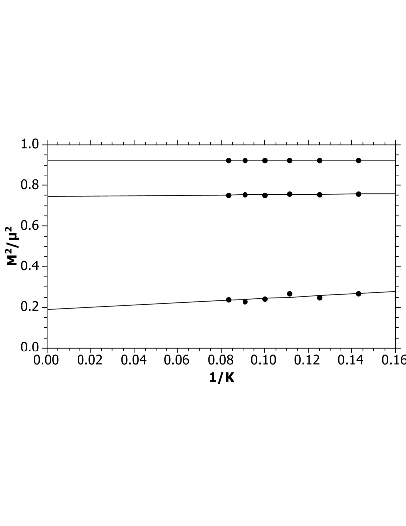
Figure 7: Lowest mass for the odd case as function of the reciprocal of the highest order $K$ of the polynomial included in the five-body Fock sector, for $g=0.5$, 1.0, and 2.0. In the three-body sector, the highest order was 15, and the Fock space was truncated at five constituents. The lines are linear fits extrapolated to infinite order.

Figure 8: Same as Fig. 7, but for the mass renormalization shift $\Delta$ and $g$ values of 0.5, 1.0, and 1.5.

Each extrapolation included an error estimate in the infinite-order intercept, and for all but the initial, top-level extrapolation, subsequent extrapolation was done with contributions weighted by their errors. The last extrapolation then yielded an overall error estimate for the final extrapolated value, and this was used for error bars in the plots of mass values. As the coupling approached the critical value, the errors grew, as would be expected, because higher Fock states become more important for the calculation, leading to a greater dependence on the basis size in higher sectors.

References

- (1) S.-J. Chang, Phys. Rev. D 12, 1071 (1975); 13, 2778 (1976).
- (2) A. Harindranath and J.P. Vary, Phys. Rev. D 36, 1141 (1987).
- (3) S. Rychkov and L.G. Vitale, Phys. Rev. D 91, 085011 (2015).
- (4) D. Lee, and N. Salwen, Phys. Lett. B 503, 223 (2001).
- (5) T. Sugihara, J. High Energy Phys. 05(2004), 007 (2004).
- (6) D. Schaich, and W. Loinaz, Phys. Rev. D 79, 056008 (2009).
- (7) P. Bosetti, B. De Palma, and M. Guagnelli, Phys. Rev. D 92, 034509 (2015).
- (8) A. Milsted, J. Haegeman, and T.J. Osborne, Phys. Rev. D 88, 085030 (2013).
- (9) For reviews of light-cone quantization, see M. Burkardt, Adv. Nucl. Phys. 23, 1 (2002); S.J. Brodsky, H.-C. Pauli, and S.S. Pinsky, Phys. Rep. 301, 299 (1998).
- (10) J.P. Vary et al., Phys. Rev. C 81, 035205 (2010).
- (11) S.S. Chabysheva and J.R. Hiller, Phys. Rev. D 84, 034001 (2011).
- (12) C. Gattringer and C.B. Lang, Quantum Chromodynamics on the Lattice, (Springer, Berlin, 2010); H. Rothe, Lattice Gauge Theories: An Introduction, 4e, (World Scientific, Singapore, 2012).
- (13) C.D. Roberts and A.G. Williams, Prog. Part. Nucl. Phys. 33, 477 (1994); C.D. Roberts and S.M. Schmidt, Prog. Part. Nucl. Phys. 45, S1 (2000); R. Alkofer and L. von Smekal, Phys. Rept. 353, 281 (2001); I. C. Cloet and C. D. Roberts, Prog. Part. Nucl. Phys. 77, 1 (2014).
- (14) P.A.M. Dirac, Rev. Mod. Phys. 21, 392 (1949).
- (15) S.S. Chabysheva and J.R. Hiller, Phys. Rev. E 90, 063310 (2014); S.S. Chabysheva, B. Elliott and J.R. Hiller, Phys. Rev. E 88, 063307 (2013).
- (16) H.-C. Pauli and S.J. Brodsky, Phys. Rev. D 32, 1993 (1985); 32, 2001 (1985).
- (17) J.S. Rozowsky and C.B. Thorn, Phys. Rev. Lett. 85 (2000), 1614; V. T. Kim, G. B. Pivovarov, and J. P. Vary, Phys. Rev. D 69 (2004), 085008; D. Chakrabarti, A. Harindranath, L. Martinovic, and J.P. Vary, Phys. Lett. B 582 (2004), 196; D. Chakrabarti, A. Harindranath, L. Martinovic, G.B. Pivovarov, and J.P. Vary, Phys. Lett. B 617 (2005), 92; D. Chakrabarti, A. Harindranath, and J.P. Vary, Phys. Rev. D 71 (2005), 125012; L. Martinovic, Phys. Rev. D 78, 105009 (2008); S.S. Chabysheva and J.R. Hiller, Ann. Phys. 340, 188 (2014).
- (18) S.S. Chabysheva and J.R. Hiller, Phys. Rev. D 79, 096012 (2009).
- (19) M. Burkardt, Phys. Rev. D 47, 4628 (1993).
- (20) I.S. Gradshteyn, I.M. Ryzhik, Y.V. Geronimus, and M.Y. Tseytlin; A. Jeffrey, D. Zwillinger, and V.H. Moll, eds., Table of Integrals, Series, and Products 8th ed., (Academic Press, New York, 2015).
- (21) S.S. Chabysheva and J.R. Hiller, Phys. Lett. B 711, 417 (2012).
- (22) B. Elliott, S.S. Chabysheva, and J.R. Hiller, Phys. Rev. D 90, 056003 (2014).
- (23) R.J. Perry, A. Harindranath, and K.G. Wilson, Phys. Rev. Lett. 65, 2959 (1990); R.J. Perry and A. Harindranath, Phys. Rev. D 43, 4051 (1991).
- (24) J.R. Hiller and S.J. Brodsky, Phys. Rev. D 59, 016006 (1998).
- (25) V.A. Karmanov, J.-F. Mathiot, and A.V. Smirnov, Phys. Rev. D 77, 085028 (2008); Phys. Rev. D 82, 056010 (2010).
- (26) S.S. Chabysheva and J.R. Hiller, Ann. Phys. 325, 2435 (2010).