Cosmological hydrodynamical simulations of galaxy clusters: X-ray scaling relations and their evolution
Abstract
We analyse cosmological hydrodynamical simulations of galaxy clusters to study the X-ray scaling relations between total masses and observable quantities such as X-ray luminosity, gas mass, X-ray temperature, and . Three sets of simulations are performed with an improved version of the smoothed-particle-hydrodynamics GADGET-3 code. These consider the following: non-radiative gas, star formation and stellar feedback, and the addition of active-galactic-nucleus (AGN) feedback. We select clusters with , mimicking the typical selection of Sunyaev–Zeldovich samples. This permits to have a mass range large enough to enable robust fitting of the relations even at . The results of the analysis show a general agreement with observations. The values of the slope of the mass – gas mass and mass temperature relations at are 10 per cent lower with respect to due to the applied mass selection, in the former case, and to the effect of early merger in the latter. We investigate the impact of the slope variation on the study of the evolution of the normalization. We conclude that cosmological studies through scaling relations should be limited to the redshift range , where we find that the slope, the scatter, and the covariance matrix of the relations are stable. The scaling between mass and is confirmed to be the most robust relation, being almost independent of the gas physics. At higher redshifts, the scaling relations are sensitive to the inclusion of AGNs which influences low-mass systems. The detailed study of these objects will be crucial to evaluate the AGN effect on the ICM.
keywords:
galaxies: clusters: general — galaxies: clusters: intracluster medium — X-ray: galaxy: clusters — methods: numerical1 Introduction
Clusters of galaxies are the largest gravitationally bound structures in our Universe and according to the hierarchical process of structure formation they are the latest to form. Due to these characteristics, they can provide stringent constraints on the cosmological parameters (such as the amplitude of the linear power spectrum, the amount of matter, and that of dark energy) that determine the growth rate of structures (e.g. Borgani and Kravtsov, 2011; Planelles et al., 2015).
In this respect, one of the most powerful cosmological measurements is the evolution of the mass function (Borgani and Guzzo, 2001; Voit, 2005; Vikhlinin et al., 2009; Allen et al., 2011). However, the measurement of cluster masses via X-ray or gravitational lensing is complicated and questioned by the presence of possible biases caused by several factors, such as lack of hydrostatic equilibrium or triaxiality. For this reason, in order to infer masses for a large number of objects, it is preferable to resort to relations between the total mass and some observable quantities that are relatively easy to measure, the so-called mass proxies (Hilton et al., 2012; Takey et al., 2013; Giles et al., 2016). From an observational point of view, these relations need to be calibrated by measuring the total masses, via weak-lensing or X-ray analyses, for a smaller, but optimal, set of galaxy clusters.
In X-ray studies, the most commonly used mass-proxies are the gas mass, , which can be extracted from the surface brightness profile, the temperature, , which is solidly estimated from X-ray spectra with, at least 1000 counts, and their combination, (e.g., Maughan, 2014; Mantz et al., 2016, for recent and detailed studies on X-ray scaling relations). The parameter was first introduced as a mass proxy closely related to the total thermal content of the intracluster medium (ICM) by Kravtsov et al. (2006). In that paper, through the analysis of hydrodynamical simulations, the authors proved the advantages of this quantity as a mass proxy over gas mass and X-ray temperature. Specifically, gas mass and temperature react in opposite directions to any breaking of self-similarity (see Section 3.2) caused, for example, by non-gravitational effects. In the computation of the product of the two quantities, the deviations from the self-similar (SS) behavior compensate each other, keeping the evolution closer to the expected (SS) one. In addition, the relation is characterized by a small scatter. Indeed, the gas mass and temperature respond in opposite ways to the effects of, e.g., mergers and energy feedback from active galactic nuclei (AGN) (Kravtsov et al., 2006; Fabjan et al., 2011). In case of an encounter, the gas mass immediately increases while the temperature, at first, decreases due to the presence of the smaller and thus colder structure (Poole et al., 2007; Rasia et al., 2011). The feedback by AGNs reduces the gas mass by expelling some gas from the core and, at the same time, it heats the ICM. These opposite and compensating responses of the two quantities make their product, , independent of the dynamical state or on the central AGN activity (see, however, Le Brun et al. 2014 for a different conclusion). For all these reasons, has been widely adopted in cosmological applications of galaxy clusters.
Another X-ray measurement frequently represented in the analysis of scaling relations is the X-ray luminosity because it can easily be derived from few tens of net photon counts (e.g. Giles et al., 2017, and references therein). The relation has been historically important because from its first determination it was clear that it provides information on the physics of the cluster core (e.g., Fabian et al., 1994) and on the phenomena of feedback by stars or AGNs (e.g., Markevitch, 1998; Maughan et al., 2012). These connections are also the origin of the large scatter of this relation as well as of the associated relation. Due to this characteristic, the appeal of as mass-proxy is limited. However, the inverted relation, i.e., between the luminosity and the mass (the relation), still plays an important role in establishing the selection function of X-ray surveys (e.g. Nord et al., 2008; Vikhlinin et al., 2009; Allen et al., 2011), since it determines the connection between the survey flux limit and the minimum mass that can be observed at a given redshift.
From this discussion, it is clear that in the past 10-15 yr, scaling relations have been largely studied in observational samples. Up to date, their analysis has rarely been extended beyond (Reichert et al. 2011; Maughan et al. 2012; Giodini et al. 2013). The collection of high-redshift systems will grow thanks to future optical missions like eROSITA111http://www.mpe.mpg.de/eROSITA(Merloni et al., 2012), Euclid222http://www.euclid-ec.org (Laureijs et al., 2011), LSST333http://www.lsst.org(Ivezic et al., 2008), and to millimetric surveys such as SPT-3G (Benson et al., 2014) and CMB-S4. These identify clusters through the small distortions of the cosmic microwave background (CMB) radiation caused by the inverse Compton scattering of the CMB photons that interact with the ICM electrons. The phenomenon, called Sunyaev–Zeldovich (SZ) effect, has already enabled the detection of a good number of objects at (Menanteau et al., 2013; Bleem et al., 2015). Once the clusters will be detected, a possible follow-up will be provided by current or future X-ray observatories, first of all, Athena444http://www.the-athena-x-ray-observatory.eu. The selection functions characterizing the samples from these future surveys are very different one from the others (Weinberg et al., 2013; Ascaso et al., 2017): the SZ-selected samples, such as those of the South Pole Telescope (SPT) or the Atacama Cosmology Telescope (ACT), extend to less massive objects at higher redshifts and, thus, are the most suitable for high-redshift searches. The limiting mass of the mentioned optical surveys, instead, will be almost constant up to and then will grow at earlier epochs. The efficiency of optical detection is, therefore, expected to drop at . Finally, the forecast for eROSITA limits the cluster discovery at because of the dimming of the X-ray emission at large distances.
Over the last decade, the theoretical community has also spent a significant effort in the modelling of scaling relations by taking advantage of hydrodynamical simulations (see Borgani and Kravtsov 2011 for a review). Special attention was dedicated to the effects of feedback from stars (Nagai et al., 2007a) and AGNs (Short and Thomas, 2009; Puchwein et al., 2008; Short et al., 2010; Planelles et al., 2014; Le Brun et al., 2014; Pike et al., 2014; Martizzi et al., 2014; Hahn et al., 2017; Gaspari et al., 2014), to the evolution of the relations up to (Battaglia et al., 2012; Fabjan et al., 2011; Planelles et al., 2017; Le Brun et al., 2016), and to developing a theoretical framework to exploit the simultaneous analysis of multiple signals (Stanek et al., 2010; Evrard et al., 2014). This paper, based on a set of simulations that includes a new model for gas accretion on to supermassive black holes and for the ensuing AGN feedback, and an improved implementation of hydrodynamics, extends the analysis of scaling relations out to in view of what future observational facilities will provide. We particularly focus on the selection function typical of SZ surveys which is demonstrated to be effective in finding high- objects (see Section 2.1).
This work analyses a set of simulations that have been shown to naturally form cool-core (CC) and non-cool-core (NCC) clusters (Rasia et al., 2015). In particular, we have already shown for these simulations that entropy, gas density, temperature, thermal pressure, and metallicity profiles of the two populations of clusters reproduce quite well observational results (Rasia et al., 2015; Planelles et al., 2017; Biffi et al., 2017). For this reason, we expect that in our simulated clusters a balance between the simulated level of radiative cooling, which forms stars, and the included amount of AGN feedback, which heats the gas, is reached as the systems evolve and interact with the cosmological environment. However, although the agreement with observations is remarkable, there still are several limitations affecting the simulations. For example, the processes linked to the stellar population and the BH activity are treated with sub-grid models, and some phenomena, such as kinetic feedback by AGNs, magnetic fields, dust production and disruption, or metal diffusion, are not implemented into the code yet. As specified in Rasia et al. (2015), this model should, therefore, be intended as effective. On the same note, as we will discuss in the next section, our sample is not a volume-complete sample. For this reason, the emphasis of our discussion is directed on the effect of the physics and on the evolutionary trends of the relations rather than on the precise values of the parameters of the best-fitting relations.
The paper is organized as follows: in Section 2, we provide a short description of the simulated sample and motivate our sample selection. Section 3 presents the computation of ICM structural quantities, the mass-proxy relations, the luminosity-based relations, and fitting methods. In Section 4, we examine the validity of our simulated data by comparing to observations at low () and intermediate () redshifts. Section 5 is dedicated to exploring the evolution of scaling relations from to . Finally, a summary of the results and conclusions are given in Section 6.
All the quantities for the scaling relations are evaluated at defined as the radius of the sphere whose mean density is 500 times the critical density of the Universe at the considered redshift. In general, is the mass of the sphere of radius and density times the critical density of the Universe at the proper redshift. The virial radius is expressed accordingly to Bryan and Norman (1998). For our cosmology, at . Throughout the paper, the symbol indicates the decimal logarithm and the uncertainty at 1 on the best-fitting parameters represents the 68.4 per cent confidence maximum-probability interval.
2 Simulations
Our analysis is based on three sets of simulations of galaxy clusters with varying sub-grid physics. These are selected from a parent DM-only cosmological volume of 1 Gpc3 (Bonafede et al., 2011)555We define , where is the Hubble constant. and re-simulated at higher resolution and with the inclusion of baryons. We compute the scaling relations at eight different times corresponding to and .
The re-simulated Lagrangian regions are chosen around the 24 most massive clusters with mass 666Friends-of-Friends (FoF) refers to the algorithm in which a pair of particles are considered to belong in the same group or object (i.e. friends) when their separation distance is smaller than a given linking length . In our simulations, the linking length is equal to 0.16 in unit of the mean separation of Dark-Matter particles. plus 5 isolated groups with . The Lagrangian regions surrounding each cluster are chosen to be large enough that no contaminating low-resolution DM particle is found out to five virial radii from the centre of each cluster. Their particles, identified at redshift , are traced back to redshift , which is about 50 Myr earlier than the starting redshift of the parent DM simulation to ensure the validity of the Zeldovich approximation. The particle number is increased to achieve a better spatial and mass resolution, furthermore, the baryonic component is added. The initial conditions for the re-simulations are produced by a zoomed-initial technique (ZIC, Tormen et al. 1997). We refer to Bonafede et al. (2011) for a full description of the re-simulation technique. The resimulations are carried out with an improved version of the GADGET-3 smoothed-particle-hydrodynamics (SPH) code (Springel, 2005) where we included a number of improvements as described in Beck et al. (2016). In short, these allow the SPH method to perform better in hydrodynamical standard tests including weak and strong shocks, gas mixing, and self-gravitating clouds.
The cosmological setting is a model with cosmological parameters consistent with the WMAP-7 constraints (Komatsu et al. 2011): , , for the primordial spectral index, for the amplitude of the power spectrum of the density fluctuations, and km s-1 Mpc-1 for the Hubble parameter. When comparing our models to observational data – presented in Section 4 – we rescale the latter to the simulated cosmology.
The Plummer-equivalent gravitational softening of the DM particles is set to 3.75 in physical units up to and in comoving units at higher redshifts. The gravitational softening of the gas (), stars (), and black hole particles () are fixed in comoving coordinates at all redshifts. The minimum value of the smoothing lengths is limited to 0.1 per cent of the gravitational softening. For the computation of SPH quantities related to the gas, we employ the Wendland interpolating kernel with neighbours (see Beck et al. 2016 for more details). The mass of the DM particle is and the initial mass of the gas particle is .
We analyse three sets of simulations. These have the same initial condition for the 29 regions, but they differ in the astrophysical processes included. Comparing the results obtained from the three sets allows us to qualitatively assess their origin. Different results among the three samples imply that the scaling relations are affected by the astrophysical phenomena diversely implemented in the three sets. Viceversa, if the results are consistent, then, the behaviour of the scaling relations is determined by gravity, which drives the interactions with the environment and the large-scale structures, and by the hydrodynamical forces that, hence, take place.
In the following, we describe the three sets, tagged as nr, csf, and agn, from the simplest to the most complex:
(i) nr (Non-radiative). These simulations are carried out with the same code used by Beck et al. (2016). The main variations with respect to the standard GADGET code include the following: the choice of a higher order Wendland kernel function; a time-dependent artificial viscosity scheme; a thermal diffusion term (or artificial conduction) that improves the treatment of contact discontinuities and promotes fluid mixing. The performance of this code with respect to other particle- or grid-based codes is described in Sembolini et al. (2016b) and Sembolini et al. (2016a). These works show how the thermodynamical properties of the ICM for the clusters simulated with the improved GADGET version (G3-XArt in those papers) are quite similar to those produced by grid codes, AREPO, and the most modern SPH schemes (Sembolini et al. 2016a).
(ii) csf (Cooling, star formation and stellar feedback). The radiative runs consider metal-dependent radiative cooling rates accordingly to Wiersma et al. (2009), where 15 different elements (H, He, C, Ca, O, N, Ne, Mg, S, Si, Fe, Na, Al, Ar, Ni) are followed; the effect of a uniform UV/X-ray background radiation (Haardt and Madau, 2001); the feedback by supernovae (SN), as originally prescribed by Springel and Hernquist (2003) with a mass loading parameter equal to 2; the chemical model by Tornatore et al. (2007) to account for the metal enrichment from SN II, SN Ia, and asymptotic giant branch (AGB) stars (for further details see Planelles et al. 2014; Biffi et al. 2017). Kinetic feedback from the outflows driven by supernova is included. The wind velocity is set equal to 350 km s-1.
(iii) agn. This set of simulations is the same as the
csf one, but with the addition of AGN feedback. This feedback
channel is modelled following Steinborn et al. (2015), who improved
the original model by Springel et al. (2005). In the
new model, we consider both radiative and mechanical feedback
generated from gas accretion on to black hole, both being released into
the surrounding gas as thermal energy. The radiative and mechanical
efficiencies depend on the (Eddington-limited) accretion rate and the
black hole mass, allowing for a smooth transition between radio- and
quasar-modes. The coupling efficiency between the energy radiated from
the black hole and the gas is expressed though the factor
. In addition, the model separately treats the
accretion of cold gas and hot gas. Only for the accretion of the cold
gas, we boost the Bondi rate by a factor of 100, so as to mimic the
effect of the cold accretion mode, as discussed by
Gaspari et al. (2017).
The thermodynamical and chemodynamical
properties, and the dynamical state of the simulated clusters of this
sample are also presented in Rasia et al. (2015),
Villaescusa-Navarro et al. (2016), Biffi et al. (2016),
Planelles et al. (2017), and Biffi et al. (2017). The
agn simulations of the main clusters of the 29 regions are
presented in Rasia et al. (2015). The entropy and iron
profiles of the CC and NCC populations are shown to agree with observational data. The observed anticorrelation
between the core entropy and core enrichment level is also
reproduced (Biffi et al., 2017). The different behaviour between
the two classes is confirmed in the pressure profiles: in the
central part of the CC systems the pressure is higher by an amount
that reflects the observational gap measured from SPT and Bolocam
data (Planelles et al., 2017). The increase in CC central thermal
pressure is larger than the deepening of the gravitational potential
arising from a more pronounced adiabatic contraction. As a consequence,
the bias in the hydrostatic-equilibrium masses measured in the core
() of CC objects is found to disappear or to be
negligible (Biffi et al., 2016).
2.1 The Sample
The sample includes all the objects in the high-resolution Lagrangian regions with where . The number of clusters in the agn run selected at the redshifts of interest and the corresponding mass range are presented in Fig. 1. In the following we will comment on the most important implications related to the sample selection.

2.1.1 The limitation on 29 Lagrangian regions
The majority of the simulated regions (24 to be precise) are centred around massive clusters. Therefore, we could expect that a good fraction of our smallest objects lies in a particularly rich environment. This condition could influence some of their properties. In particular, these systems might be subject to gas depletion or over-heating. We check whether any of these two conditions are present in our sample by comparing the results of the nr set with those obtained by Le Brun et al. (2016), who analysed a cosmological box. We selected the NR runs to avoid the comparison between samples simulated with different ICM prescriptions. We found that their best-fitting relations are passing through the middle of the distribution of our clusters in both the () and () planes and at both redshifts, and . We conclude that our smallest objects are not particularly gas poor or unusually hot for their mass, and thus are representative of the object population in the lowest mass bins. To further prove this point, we study the behaviour of the five groups at the centre of the remaining Lagrangian regions. These objects do not have a massive cluster in their vicinity and have a small mass, two of them are close to our limiting mass. All five groups are located in the middle of the distribution of our entire sample in all of the runs.
2.1.2 The upper mass limit
Another concern, linked to the restriction of the volume analysed, is connected to the representativeness of our most massive systems at higher redshifts.
The upper mass limit shown in Fig. 1 represents the mass of the most massive system found at each redshift. This value might also be affected by the restriction of our study to 29 Lagrangian regions especially at high redshift. Indeed, in our study, we automatically include all the progenitors of our sample and exclude all objects outside the high-resolution resimulated region. It is expected that most of the progenitors of massive objects are still massive at or above. Although, it might be that a halo considered very massive at stops its growth and remains of about the same mass at (see Fig. 7 in Muldrew et al., 2015). This could happen if the accretion was as fast and intense as to conglomerate into the object most of the surrounding material and to create an under-dense region all around. That cluster, which was one of the most massive ones at high redshift, will become a relatively small object with respect to the entire cluster population at . Because of that, it most likely could be excluded by our selection based on masses. This explains the concern of missing some of the most massive clusters.
To evaluate the extent and consequences of this aspect, we computed the predicted number of clusters above a certain mass at different redshifts by using HMFcalc (Murray et al., 2013). We consider the functional form of the Halo Mass Function proposed by Watson et al. 2013 using the formulation that includes the redshift evolution. We further set the cosmology according to the cosmological parameters of our simulations. We forecast that the parent box, with a volume of (1 Gpc)3, at , , and should have at least four objects with mass , respectively, above , , and . In our sample, above the same mass limits there are three clusters at and and two systems at . Considering the Poisson errors, these numbers are consistent with the expectation.
Therefore, we conclude that even if we are not considering a volume-limited sample at , there is a statistically good representation of massive objects among the clusters selected within the 29 Lagrangian regions. This allows us to study the scaling relations over a sufficiently large mass range, which spans from a factor of 10 at to at .
2.1.3 The lower mass limit and the variation with redshift
The lower mass limit of our selection reproduces the same dependence on as of the SZ-selected clusters (e.g. see fig. 6 from Bleem et al., 2015, for the SPT sample). Our choice is aimed at maximizing the statistical size of our simulated sample and enlarging the mass range in order to robustly derive the scaling relations in single redshift bins.
Indeed, applying to our 29 Lagrangian regions the selection functions typical of X-ray or optical surveys, whose lower mass limits are, respectively, increasing and nearly constant with redshift, would have returned a poor statistics, especially at high redshift. Looking at specific future surveys of clusters, we recall that the limiting mass of the selection function of eROSITA (Borm et al., 2014) rapidly grows with redshift from at to at , while that of Euclid (Sartoris et al., 2016) will be almost constantly equal to from to and will grow afterwards. Considering the rapid decline of the cosmological mass function, these missions will not cover as large mass range as future SZ surveys.
Our high-redshift samples, i.e. at , , and , include 74, 60, and 36 objects, respectively, numbers comparable to studies on local observed scaling relations, and, as previously said, extend in mass by a factor ranging from almost 5, at , to 10, at .
The smallest system at contains more than particles providing good estimates of global quantities. We do not extend the sample to smaller systems, even if we would have obtained numerically robust global measures, because, again, none of the planned missions will reach such small masses.
As we will further discuss in the next sections, our choice will have some impact on the computed evolution of the scaling relations. In fact, our selection excludes at the smallest groups of galaxies, that are known to cause a break of the power-law fitting of the and relations. We will, therefore, model these relations as single power laws, thus avoiding a more complicated parametrization (see, however, the detailed analysis performed by Le Brun et al. 2016). The same benefit is nevertheless not present at high redshifts, when the SZ selection is indeed sampling smaller mass systems, which are affected by a drastic reduction of the gas fraction (Dai et al., 2010). The scaling relations involving the gas mass can still be fitted by a single power law – since less massive objects will be present at but the overall sample population will be different (see Section 5.1).
3 Method of Analysis
3.1 Computing ICM Quantities
In the following, we briefly describe how we compute the relevant quantities from our simulated data sets.
Masses. The total mass, , is calculated by summing the contribution of all the species of particles (dark matter, gas, and stars) within . For the gas mass, , we sum the hot gas component. In the case of multicomponent particles777The gas particles can be multi-phase, carrying information on both the hot and cold gas. The cold phase provides a reservoir for stellar formation., we include all particles containing less than 10 per cent of cold gas, and therefore no star-forming particles. In each region, the mass of the hot gas contained in all the particles with a cold gas fraction larger than 10 per cent is less than 0.01 per cent of the total hot gas of the region, and thus is negligible.
Temperature. We consider both the mass-weighted temperature and the spectroscopic-like temperature (Mazzotta et al., 2004). To compare with observations (Section 4) we consider the same aperture used in the observational samples (), while to derive our results (Section 5) we exclude the contribution of the core, defined as the region within 15 per cent of ().
The mass-weighted temperature is provided by
| (1) |
where and are the hot-gas mass and temperature of the gas particle. The spectroscopic-like temperature is introduced to ease the comparison with X-ray observations and the formula was derived considering the non-flat response of the instruments on board of Chandra and XMM–Newton:
| (2) |
where is the particle gas density (Mazzotta et al., 2004, see also Vikhlinin 2006). For this computation, we used only particles emitting in the X-ray band with keV.
The parameter . As previously said, this parameter is equivalent to the product of the gas mass and the core-excised temperature within and it is a powerful proxy for the total thermal content of the ICM because it is almost insensitive to the physical processes included in simulations (Stanek et al., 2010; Fabjan et al., 2011; Battaglia et al., 2012; Sembolini et al., 2014) and to the dynamical status of the clusters (Poole et al., 2007; Rasia et al., 2011; Kay et al., 2012). is derived from X-ray observations, and therefore we adopt the core-excised spectroscopic-like temperature in its expression:
| (3) |
As specified above, in Section 4 the observational quantities, which we compare to, are available only within the fixed aperture of (Mahdavi et al., 2013, and its erratum), therefore, exclusively in that section and in Figures 2 and 3, we compute without excising the core.
X-ray Luminosity. The bolometric luminosity is computed by summing the contribution of the emissivity, , of all gas particles within the sphere of radius :
| (4) |
where , are number densities of electrons and hydrogen atoms, respectively, is the particle’s volume and is the interpolation of the cooling function pre-calculated in a fine grid of temperatures and metallicities starting from the values of temperature, , and global metallicity, , of each gas particle888We recall that, in our simulations, the ratios of the abundances of the elements such as oxygen or silicon over the iron abundance are typically close to the solar value (Biffi et al., 2017). Furthermore, the influence of boosted single element line does not substantially increase the bolometric luminosity.. The cooling-function tables are created by assuming the APEC model (Smith et al., 2001) in XSPEC and by integrating over the keV energy band.
3.2 The scaling relations and the self-similar prediction
The total mass of a cluster can be related to the various ICM quantities presented in the previous sections through simple power-law models. Kaiser (1986) analytically derived the functional shapes of the expected scaling relations under the assumption of virial equilibrium between the kinetic and thermal energy of a galaxy cluster and its gravitational potential (a recent extension of the formalism is provided in Ettori, 2015). According to this model, called SS, the cluster total mass is the only parameter that defines both thermal and dynamical properties of the ICM (e.g., Giodini et al. 2013 and references therein). Clusters with different mass are simply the scaled-up or -down version of each other. The self-similarity stems from the fact that there is no preferred scale in the problem as gravity and the initial power spectrum are scale-free (or SS). In this context, the total mass is the only variable of the problem. For this reason, the scaling relations are often presented with the mass as independent variable, especially in theoretical and numerical studies. However, from a practical and observational perspective, the scaling relations are adopted to derive the total mass of the clusters once the mass proxy quantities are measured. We will resort to this presentation for all relations linking the total mass to a mass-proxy (, , and ). On the other hand, we will also consider the and relation with the bolometric luminosity as dependent variable because both relations are observationally used to derive the flux limit corresponding to a certain mass or temperature.
In the following, we will describe the mass-proxy relations (1, 2, and 3) and the luminosity-based relations (4 and 5) together with their expected dependence with redshift parametrized as power of valid for a background cosmology (see e.g., Borgani and Kravtsov 2011). Note that in Kaiser (1986), the redshift evolution was modelled in terms of powers of as expected for an Einstein-de-Sitter Universe. In all relations, we treat the normalizations, , as constants, although in general they depend on the internal structure of the system.
(1) The relation. The total mass and the gas mass are linearly related:
| (5) |
without any dependence on redshift.
(2) The relation. The total mass is related to the temperature according to:
| (6) |
(3) The relation. From Eqs. 3, 5, and 6, the self-similar scaling of with cluster mass is given by
| (7) |
(4) and (5) The luminosity relations: and . Assuming thermal bremsstrahlung emission, the bolometric luminosity can be related to the total mass by
| (8) |
where is the gas fraction. Given the expression of the and relations (equations 5 and 6), the self-similar form for the relation is expressed as
| (9) |
and for the relation as
| (10) |
3.3 Fitting Method
| Relation | |||
|---|---|---|---|
| 1 | 0 | ||
| 3/2 | -1 | ||
| 3/5 | -2/5 | ||
| 2 | 1 | ||
| 4/3 | 7/3 |
To study the evolution of the parameters of the scaling relations, we fit them through a generic expression:
| (11) |
can either represent the total mass, , or the X-ray luminosity, . In the first case, is assumed to be one of the mass proxies: , , , . In the second case, stands either for the spectroscopic-like temperature or for the total mass. The value of each pivot point, , is listed in Table 1. These are independent from to facilitate the study of the evolution of the normalization. The values of the pivot points are close to the median values of the variables (, , , , and ) of the entire agn sample that includes the objects from all the redshifts. At first, we fix to the SS expectation values (also listed in Table 1) and we derive and at each independent redshift (Sections 5.1 and 5.2). Later, to study the evolution of the normalization, we let free to vary (Section 5.3).
We used three different algorithms implemented in IDL routines to fit the data. Two of them are robust statistical methods commonly used in recent observational studies (see Sereno, 2016, for a review) while the last method is more appropriate to analyse data from numerical sets where the two variables are independently derived and their calculation does not have any associated error. We found that the best-fitting parameters derived from the three techniques agree within 1 . Therefore, we will show the exact values obtained only from the third method with only the exception of the results in Section 5.3 where we are forced to use the first program (see below). The IDL routines employed are as follows:
(i) linmix_err.pro adopts a Bayesian approach described in Kelly (2007) to investigate the parameter space and to perform the linear regression in logarithmic space. The routine is applied to the single linear regression with , , and the intrinsic scatter as free parameters. This method allows us to treat the intrinsic scatter, , estimated via the method of Monte Carlo Markov Chains, as a free parameter. Exclusively, when we treat as an additional free parameter (Section 5.3), we use the mlinmix_err.pro routine to adopt a fitting function that is not a simple power law.
(ii) bces.pro is a least-squares bisector method (Isobe et al., 1990) that applies a linear regression that accounts for any possible correlation between the errors associated with the two variables and the intrinsic scatter in the data (Akritas and Bershady, 1996).
(iii) robust_linefit.pro (with the bisector flag switched on) uses a two-variable linear regression and does not make any distinction between dependent or independent variables. As the others, it controls the influence of outliers. For all these characteristics, we consider this as the most suitable approach for our analysis. The best-fitting parameters derived with this method and the previous one do not have any error associated. To estimate their uncertainty, we apply a bootstrapping method with iterations. The best-fitting parameters and their uncertainties are the means and standard deviations of the distributions derived from this technique.
4 Comparison between simulated and observed scaling relations
4.1 Observational data sets
In this section, we qualitatively compare our theoretical predictions for the scaling relations to some observational results. For the mass-proxy relations, due to uncertainties associated with the amplitude of the X-ray hydrostatic mass bias derived both in observations (von der Linden et al., 2014; Maughan et al., 2016; Khatri and Gaspari, 2016) and simulations (Nagai et al., 2007b; Rasia et al., 2012; Biffi et al., 2016), we prefer to refer to masses estimated via the gravitational lensing technique. More specifically, we refer to Lieu et al. (2016) and Mahdavi et al. (2013). Nevertheless, we remark that potential biases in weak-lensing mass measurements are also present (Meneghetti et al., 2010; Becker and Kravtsov, 2011; Bahé et al., 2012). Indeed, the weak-lensing masses of the last sample were corrected in a subsequent study from the same group (Hoekstra et al., 2015).
Lieu et al. (2016) performed weak-lensing analysis of 38 clusters out of the 100 brightest clusters of the XXL survey (Pierre et al. 2016) to derive their lensing masses using the Canada–France–Hawaii Telescope Lensing Survey (CFHTLenS, e.g. Heymans et al. 2012; Erben et al. 2013) shear catalogue. The X-ray temperatures of the 38 clusters are measured by the telescope in a central region (within kpc). To compare with them, we also calculated the spectroscopic-like temperature within the same aperture.
The second sample contains 50 galaxy clusters in the redshift range . The optical data are taken from the Canadian Clusters Comparison Project (CCCP; see Mahdavi et al. 2013; Hoekstra et al. 2015), while the X-ray properties are based on the combined data from the Observatory and the telescope. In the following and in the figures, we consider the values taken from the tables provided in the erratum by Mahdavi et al. (2014).
4.2 Comparison to observations at local and intermediate redshifts
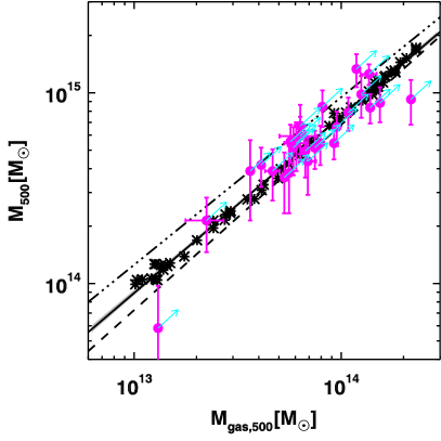
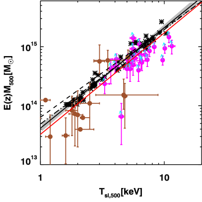
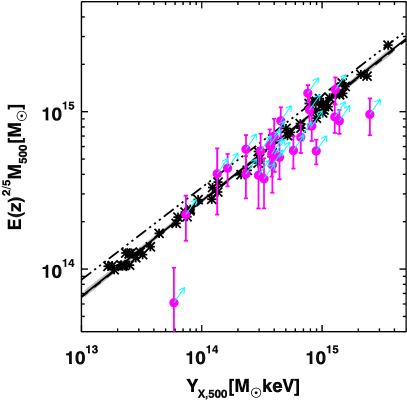
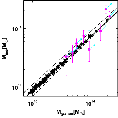
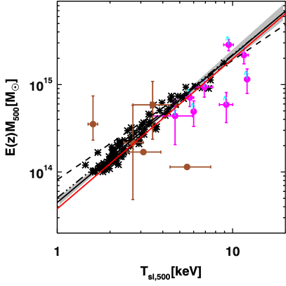
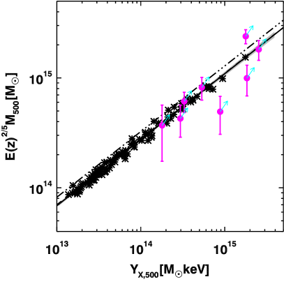
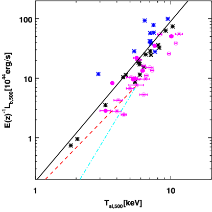
We present the comparison between our agn-simulated scaling relations and those obtained from observational samples. We stress that this comparison can only be qualitative since all samples are differently selected. The simulations at are associated with observed clusters at in Fig. 2, while the simulated set is matched to a sample of objects with redshift between 0.42 and 0.55 with median values equal to 0.5 in Fig. 3. Each figure shows four scaling relations: , , , and . In this Section, all properties are measured within without any core excision in order to be consistent with the observed quantities. For the comparison, the observational measurements of , , and , which depend on , and , respectively, have been rescaled according to the value of the Hubble parameter of the simulation.
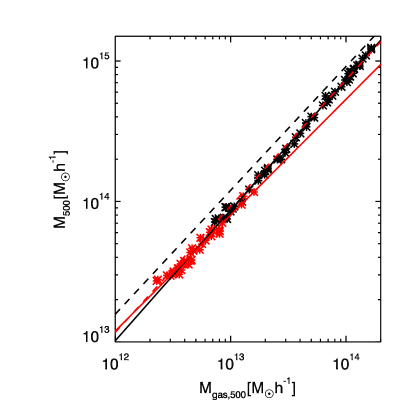
In general, we observe a good consistency between simulations and observations for the three relations , , and , especially considering that the Mahdavi et al. (2013) measurements of the masses should be increased by per cent accordingly to the revised work from the CCCP group (Hoekstra et al., 2015). In the most recent paper, the authors provide new measurements after accounting for several corrections of key sources of systematic errors in the cluster mass estimates. Unfortunately, they did not present the updated values of the X-ray quantities which might change because of the different radius related to the new mass profile. Using our agn sample, we estimate that a variation in mass of 25 per cent corresponds, on average, to an increase of gas mass, temperature, and bolometric luminosity of about 25, , and 5 per cent, respectively. These changes are represented by the cyan arrows in the figures.
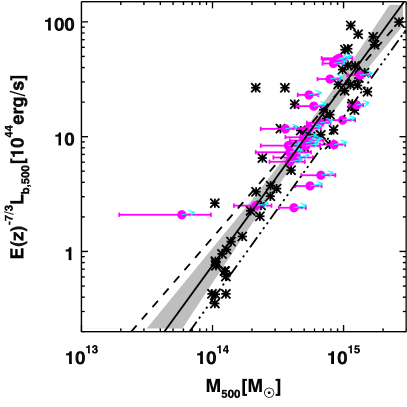
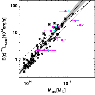
The good agreement in the normalization of the relation assures that the simulated gas fraction is realistic over the mass range investigated. However, our agn–simulated clusters appear to be colder than those at the same mass obtained from observations. At fixed mass, the temperatures of Mahdavi et al. (2013) are higher than our simulated values by about per cent ( per cent) at (). This discrepancy is reduced to 12 per cent once we considered the corrected values of total mass (Hoekstra et al., 2015) and the estimated correction for the temperature. In the low-mass range, we also observed a temperature discrepancy of in comparison to Lieu et al. (2016) at . We recall that the temperature in this work (brown circles in the figures) is measured within an aperture of kpc rather than within . The data points should then be compared with the simulated relation, shown in the figures with a red line. Comparing with this line, we found 1 consistency between our best-fitting relation and that of Lieu et al. (2016)’s. In the luminosity–mass plane, our agn simulated clusters lie in the same region of the observed data. We notice, however, that at fixed mass, some of the observed clusters are less luminous than all our simulated clusters. This leads to an offset of 30 per cent in the normalization. A possible explanation could be an overly-peaked gas distribution in the simulated sample. However, the gas fraction profiles of our simulated clusters are in good agreement with observations (Simionescu et al., 2017) and we believe that this effect, if in place, could play only a minor role. The majority of this discrepancy, instead, is likely due to the different sampling choices, related for example to the dynamical state of the clusters and to a diverse procedural treatment of the simulated and observed data. In our analysis, indeed, we do not mask any sub-clumps present within . For example, we verify that two simulated objects that in Fig. 2 are a factor 6-8 more luminous than the overall (either observed or simulated) population are experiencing a major merger with a substructure that already crossed of the main haloes. The luminosity of these two clusters is, thus, boosted (Torri et al., 2004) by the additional contribution of the large merging system, which would be removed in any observational analysis.
To investigate in a deeper manner the influence of the central regions, we compare the relation measured in the two categories of cool-core and non-cool-core (Fig. 4) clusters. The two simulated classes are taken from Rasia et al. (2015) and refer to the main haloes of the 29 re-simulated regions. The distinction between the two classes was established on the basis of the pseudo-entropy level of the objects, which is derived through the following expression:
| (12) |
where the spectroscopic like temperature, , and the emission measure, , are computed in the region, , and in the region, . We apply the cut of to define CC clusters. Those with larger values are classified as NCC clusters.
Overall, the simulated relation is in line with the observed scaling, in particular in terms of the slope. There is an offset in the normalization of slightly less than 50 per cent, which is mainly produced by the combination of simulated lower temperatures and slightly higher luminosities. Nevertheless, it is reassuring that, as found in observations, the simulated CCs (blue) tend to have larger luminosities than the NCC (black) systems due to a denser core that produces a more peaked surface brightness profile. To illustrate the effect of the physics of the AGN feedback model, we overplot in Fig. 4 the results from very high-resolution ideal hydrodynamical simulations which can isolate the impact of two major modes of AGN feedback (cf. Gaspari et al. 2014), namely tightly self-regulated AGN feedback (dashed red line) and a thermal quasar blast (dashed–dotted cyan line). The self-regulated AGN feedback (typically mediated via chaotic cold accretion on to the super massive black hole, Gaspari and Sa̧dowski 2017) tends to preserve the long-term CC structure, only mildly steepening the cluster ; it has been shown to be crucial to reproduce several properties of hot haloes, including gently quenching cooling flows (e.g., McNamara and Nulsen 2012 for a review). The quasar blast instead promotes a drastic overheating/evacuation (already at the poor cluster regime), raising the cooling time above the Hubble time and rendering most of the low-temperature system NCCs, which is inconsistent with data (e.g., Sun et al. 2009, Hudson et al. 2010, McDonald et al. 2013). In this case, the luminosity is rapidly growing with the temperature (). Our sample never experiences such a steep relation, not even at . The presence of cool cores in combination with a reasonable relation implies that a regulation of the cooling-heating balance is effective in our simulations since the collapse of the systems. Our effective AGN subgrid model seems to be closer to the gentler self-regulated AGN feedback evolution, preventing a strong evacuation of the central gas. We remark that preserving quasi thermal equilibrium of hot haloes, as observed, is a major and difficult constraint to obtain in simulations, which often display either overcooling (e.g., Hahn et al. 2017) or overevacuation (e.g., Puchwein et al. 2008).
5 Evolution of ICM Scaling Relations
In this section, we explore the evolution from up to of the six scaling relations: , , , , , and . We will discuss in more detail the scaling relations involving the gas mass and temperature since all the others are tightly connected to these.
We remind that in this section all the temperatures are obtained excluding the central region ( ). We will comment on the effect of the exclusion/inclusion of the core but we anticipate that excising the core produces a minimal variation. Indeed, the temperature difference is below 1 per cent in our agn sample and below 2 per cent in observational samples (Maughan et al., 2012) once we compare the temperature measured in the entire sphere within or excising the inner core region. Nevertheless, we decided to follow the standard choice, made to avoid the influence of the uncertainties related to the status of the core (i.e., presence of CCs or NCCs) on the evolution study.
We apply the fitting procedures described in Section 3.4 and we use the fitting function expressed by Equation (11), and the pivot points listed in Table 1. The parameter of the evolution, , is here fixed to the SS expectations introduced in Section 3. The results, in terms of best-fitting parameters and 1 uncertainties, are related to the robust_linefit method and are reported in Tables 2 and 3 for all relations, ICM physics treatments, and for different redshifts.
5.1 The Slope
The evolution of the slopes of the scaling relations, , is shown in Fig. 5 for all six scaling relations and ICM physics. For the following discussion, we remind that the expected values of the fitting parameters for the SS predictions are listed in Table 1.
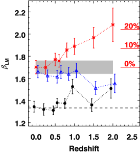
(1) The relation.
We observe that the three
runs produce shallower gas slope than the SS prediction
(). The NR value is mildly lower (2-3 per cent) than the SS
value mostly due to the fact that smaller mass systems can lose a
fraction of their gas as a consequence of violent major encounters.
This finding is not related to the sample selection applied as we
explained in Section 2.1, indeed, also in the non-radiative
cosmological box of Le Brun et al. (2016) they found that the
relation has a slope equal to 1.02, which corresponds to 0.98
once the relation is inverted to be compared with ours. We confirm
previous results from the literature that compared radiative and
non-radiative runs and find that the slope in the radiative runs is
significantly smaller ( per cent) than one
(Stanek et al., 2010; Battaglia et al., 2013) due to the conversion
of part of the hot gas into stars by the process of radiative cooling
which is more efficient in low massive systems.
The relation is approximately constant over time for the nr run (see Table 2) confirming the expectations: the total mass and the gas mass grow simultaneously. Indeed, dark matter and gas increase in mass by the same fraction when the mass growth happens via slow accretion (due to constant ratio between the densities of the gas and DM components in the cluster outskirts, e.g., Rasia et al. 2004) or via major mergers (due to a relatively constant gas fraction in system of comparable mass, e.g., Planelles et al. 2013; Eckert et al. 2016, and reference therein). For this reason, the slope of the nr run is very close to 1 and does not significantly evolve with time.
As for the radiative simulations, the csf set presents a regular shift of the relation towards higher normalization as redshift decreases (see the shift from the red dashed line for clusters to the black dashed line for objects in Fig. 6), but there is no drastic change in the slope value (see also Fig. 5). This is caused by the continuous reduction of the gas content for the active stellar production that consumes some of the hot gas. On the other hand, when the AGN feedback has been effective for some time, it maintains a higher level of hot gas. Clearly, the AGN feedback is able to effectively balance the radiative cooling and thus to prevent the overcooling and the consequent removal of gas from the hot phase, which characterize the csf runs. The impact of AGN feedback, however, depends on the cluster mass, and thus introduces a modification of the slope as we will further discuss in the following.
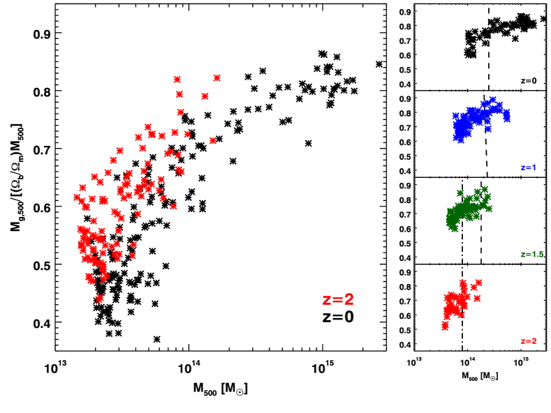
Looking at Fig. 5, we notice that no significant evolution is measurable in the agn runs from to (in agreement with previous analyses by Fabjan et al. 2011 and Battaglia et al. 2013). At , indeed, is just 2.5 per cent lower than at . However, the value of the agn slope, , decreases at and even more at to a maximum difference of with respect to . This discrepancy is statistically robust and significant at more than 2. To explain the origin of this behaviour we refer to Fig. 7 where we show the trend of the baryon fraction with the total mass at different redshifts and thus we enhance both the dependence in time of the relation as well as the impact of the SZ cluster selection which varies with (see Section 2.1). In the large panel, we show all the clusters with mass above at in black and in red. In the smallest panels, we plot the samples considered in this work at four different redshifts: and . As known from observations, the gas fraction is almost constant for masses while it decreases with decreasing total mass, below that limit. This trend seems to be present throughout the cosmic time and not much variation is detected, except a slightly higher value of the gas fraction at the highest redshifts at fixed mass. As previously pointed out, the dependence of the baryon fraction with the cluster total mass is a particular feature generated by the AGN feedback. In its absence, the baryon fraction has a constant value from groups to clusters (e.g., Stanek et al., 2010; Planelles et al., 2013). For this reason, the SZ-like selection does not impact the evolution of the slopes of either the nr or the csf runs. On the other hand, the agn sample is almost entirely on the declining part of the relation, while the local-universe sample contains a large number of clusters that are located in the plateau region. In other words, the slopes of the relations at and are influenced by the mass range covered by the sample of clusters. This depends on the SZ-like selection and it might affect also the current and future SZ analysis. Indeed, the vertical lines in the smallest panels of Fig. 7 approximately show the mass limits of the selection function of SPT and SPT-3G.
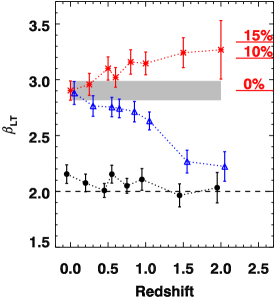
(2) The and relations.
Non-radiative runs show a slope consistent at
1 with the SS-predicted value of for all redshifts
below 1. In the radiative simulations, instead, the efficiency of the
process of radiative cooling, which cools the dense gas to produce
stars, depends on the system mass, being stronger in the low-mass
systems. The removal of this low entropy gas from the hot phase leads
to higher temperatures in groups, and thus to a steeper slope
in the csf and agn runs.
As expected, we do not find a significant difference in the values of the slope of the agn scaling relations obtained by including the core in the computation of the temperatures. The slopes, indeed, are consistent within 1 with those reported in Table 2 and have a maximum difference of 2.5 per cent at and , otherwise they change by less than 1.5 per cent. Most importantly, they present the same trend shown in Fig. 5 and detailed in the following.
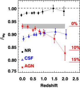
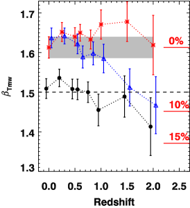
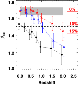
The slopes of both temperature relations, and , drop at high redshifts. The values of at are reduced with respect to the slope by , , and per cent in the nr, csf, and agn runs, respectively. The decrease in the slope is present for all the prescriptions of the ICM physics. This indicates that the origin of the variation is due to macroscopic events, linked to the global evolution of the clusters. The same trend is found in the clusters extracted from the cosmological box (of size Mpc) of the Magneticum simulations999http://c2papcosmosim.srv.lrz.de/map/find. (Dolag et al., 2016; Ragagnin et al., 2017) at redshifts and . As a further confirmation that this finding does not depend on the SZ-like selection, we explore the slope evolution for the relations derived from all objects that at each redshift are above . We find the same result as presented in Fig. 5.
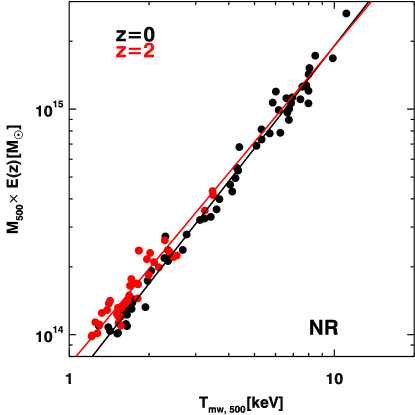
To facilitate the explanation of this result, we plot in Fig. 8 the relation for the nr clusters at and . We chose this comparison, despite its mild variation (less than 10 per cent), to better describe the variation of the thermal content (linked to rather than ) as consequence of gravitational interactions more than of radiative physics. As expected, the kinetic energy of the hot gas is not yet converted in thermal energy in high-redshift clusters, and therefore they typically exhibit a lower value of temperature at fixed total mass, i.e. for the temperatures (red points) are systematically on the left side of the ones (black points). The same result was enlightened in fig. 5 of Le Brun et al. (2016), where they show how the ratio of the kinetic energy over the thermal energy decreases with time considering various mass bins of simulated clusters extracted from a cosmological volume. We confirm the same trend of the energy ratio in our simulations (not shown). The phenomenon is present in the entire mass range but it is less pronounced for the three most massive systems at that, indeed, lie extremely close to the black solid line representing the scaling relation. These three objects have recently experienced a major merger. As a consequence, their mass has doubled (notice the mass separation from the rest of the sample), and their gas has been strongly heated by the induced shocks. To secure that our result was not influenced by the limited number of objects, we verified which fraction, among the highest mass systems in the MUSIC-2 sample101010http://music.ft.uam.es (Sembolini et al., 2013, 2014), has recently experienced a major merger. We found that this condition is verified for 10 systems out of the 11 objects with mass . We conclude that if a system about that mass threshold is already present at it is extremely likely (90% probability accordingly to the MUSIC sample) that it just went through a major merger phase that, generating strong shocks, heats the gas with a temperature enhancement which is greater than the variation of the total mass elevated by the power (see also Rasia et al., 2011). To summarize, we expect that while small clusters are still cold for their potential well, the largest objects are already located in the scaling relation because of shock heating due to minor and major mergers. This causes a shallower slope in the relation. The presence of a significant amount of cold gas in low-mass objects affects more the spectroscopic-like estimate of the temperature that, indeed, shows a stronger evolution.
The change in slope is less prominent in the agn runs. In this circumstance, the gas of the smallest systems at is warmer because of the recent and intense AGN feedback activity. The phenomenon brings the smaller objects closer to the relation reducing the amplitude of the slope evolution in the case, and even cancelling it for the relation.
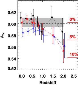
(3) The relation.
All runs at have a
slope close to the predicted SS slope of because of the
opposite deviations of and from their
SS relations as a response to the changes of the ICM
physics. In particular, the nr and agn runs are consistent
within 1 to the SS values while the of the
csf runs is per cent below.
The slope of the relation is constant until and then shows a mild decrease (between 5 and 10 per cent) for the radiative runs consistent with previous results by Sembolini et al. (2014) and by Pike et al. (2014). We notice, also, that the variation of the agn slope between and is less than 2 per cent and the two values are consistent at 1. The origin of this variation can be understood by decomposing the slope into the two slopes of the and (Maughan, 2014):
| (13) |
The complete derivation is presented in the Appendix. The mildness of the deviation is generated by the fact that none of the ICM physics runs present a coincident strong variation in both and . The nr and csf runs have the largest changes in but they have a constant , viceversa, the change in for the agn run is accompanied by the mildest drop of the value. From equation 13, it is also clear why the value of the slope is independent from the ICM prescriptions. Indeed, by comparing the agn and nr results of the slopes on the and relations, we can notice that the agn runs have lower but higher , because in the agn runs the smallest systems, at fixed total mass, have smaller gas mass but higher temperature with respect to the other ICM physics (see also discussion in Fabjan et al. 2011). This feature makes the relation the most suitable for cosmological studies that might include clusters presenting various astrophysical properties (see also Biffi et al., 2014).
(4) and (5) and relations.
Both
radiative runs exhibit significantly steeper
luminosity-temperature and luminosity-mass slopes compared with the SS
values of and , respectively. The deviation is caused by the
removal of dense gas in small clusters and groups due to efficient
radiative cooling (see above).
By including the core, we notice overall steeper slopes. However, the absolute difference in terms of slopes is less than 1 per cent for all redshifts with the exception of where it is below 3 per cent. All the values obtained by including the core are in any case consistent within 1 with those in Table 3.
In the csf runs, the slopes of the and relations respectively decreases by and 6 per cent at with respect to , while for the agn sample the same grow by 12.5 and 22.5 per cent. These changes can be again explained by the decomposition of the luminosity-based relations’ slopes:
| (14) |
| (15) |
In the first case, and carry a similar weight leading to a counterbalance between concurrent changes. In the second case, is the dominant factor, implying a variation whenever this occurs in the relation. Therefore, the steepening of the relation at is also due to the gas depletion within the potential well of small mass systems caused by the gas expulsion caused by the AGN at even higher redshifts.
Another notable feature in the luminosity relations is the separation of the slope values among the three versions of baryonic physics. The slope has a SS behavior for the nr simulations while and increase by and 25 per cent, respectively, in the radiative runs. The change is consistent with the previous argument on the gas fractions: feedback processes reduce the amount of gas in the simulated smallest systems and, thus, their total luminosity, similarly to what happens in real systems. The removal of dense gas in the smallest systems, in the csf sample is more evident at low redshift when the powerful radiative cooling cannot be regulated only by stellar feedback. On the other hand, in the agn runs, the phenomenon is more prominent at high redshifts because of the stronger AGN feedback. The gap between the agn normalization is already well established at implying that at that epoch the stellar and AGN feedback in our simulated Universe already had a significant impact in establishing the energetics of clusters. Indeed, the AGN need to eject the gas from the progenitors of groups and clusters at for getting their baryonic content and ICM properties right at lower redshift (see e.g. McCarthy et al., 2011; Biffi et al., 2017, but see also Pike et al. 2014).
| NR | CSF | AGN | ||||||||||
| z | ||||||||||||
| 0.0 | ||||||||||||
| 0.25 | ||||||||||||
| 0.5 | ||||||||||||
| 0.6 | ||||||||||||
| 0.8 | ||||||||||||
| 1.0 | ||||||||||||
| 1.5 | ||||||||||||
| 2.0 | ||||||||||||
| NR | CSF | AGN | ||||||||||
| z | ||||||||||||
| 0.0 | ||||||||||||
| 0.25 | ||||||||||||
| 0.5 | ||||||||||||
| 0.6 | ||||||||||||
| 0.8 | ||||||||||||
| 1.0 | ||||||||||||
| 1.5 | ||||||||||||
| 2.0 | ||||||||||||
| NR | CSF | AGN | ||||||||||
| z | ||||||||||||
| 0.0 | ||||||||||||
| 0.25 | ||||||||||||
| 0.5 | ||||||||||||
| 0.6 | ||||||||||||
| 0.8 | ||||||||||||
| 1.0 | ||||||||||||
| 1.5 | ||||||||||||
| 2.0 | ||||||||||||
| NR | CSF | AGN | ||||||||||
| z | ||||||||||||
| 0.0 | ||||||||||||
| 0.25 | ||||||||||||
| 0.5 | ||||||||||||
| 0.6 | ||||||||||||
| 0.8 | ||||||||||||
| 1.0 | ||||||||||||
| 1.5 | ||||||||||||
| 2.0 |
| NR | CSF | AGN | ||||||||||
| z | ||||||||||||
| 0.0 | ||||||||||||
| 0.25 | ||||||||||||
| 0.5 | ||||||||||||
| 0.6 | ||||||||||||
| 0.8 | ||||||||||||
| 1.0 | ||||||||||||
| 1.5 | ||||||||||||
| 2.0 | ||||||||||||
| NR | CSF | AGN | ||||||||||
| z | ||||||||||||
| 0.0 | ||||||||||||
| 0.25 | ||||||||||||
| 0.5 | ||||||||||||
| 0.6 | ||||||||||||
| 0.8 | ||||||||||||
| 1.0 | ||||||||||||
| 1.5 | ||||||||||||
| 2.0 |
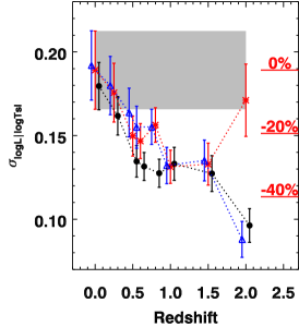
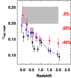
5.2 The Intrinsic Scatter
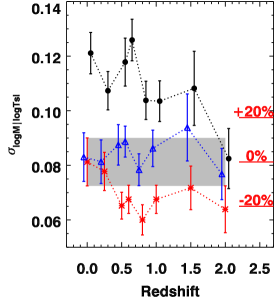
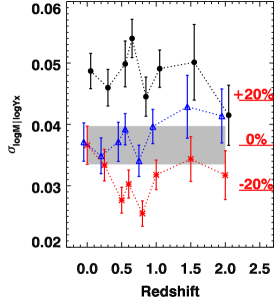
We compute the scatter, , defined as the mass variance in the decimal logarithm at fixed signal () for the mass-proxy relations and as the luminosity variance in the decimal logarithm at fixed and for the remaining relations. Using the same syntax of Equation 11, the scatter can be computed as
| (16) |
where is the number of clusters in the redshift bin and represents either the total mass or the bolometric luminosity of each object. The resulting scatter is fully consistent with the scatter value returned by the routine linmix_err.pro. The two values are, indeed, only a few per cent different between each other, with an absolute maximum variation below 0.01, meaning that this quantity is robustly defined for our samples.
In Fig. 9, we report its evolution for all our scaling relations. In addition, we evaluate the scatter measured at fixed mass or fixed luminosity. Both scatter values can be found in the last two columns for each physics of Tables 2 and 3. As often stressed in the paper, we remind that our analysis focusses on the relative trend of the scatter rather than its absolute calibration. Indeed, the latter might depend on the size of the sample considered. We do not have hundreds of objects as we would expect from selecting all the clusters in the entire cosmological box of 1 Gpc, and therefore we are unavoidably limiting the presence of outliers. The expectation is that the scatter from our sample is biased low. Nevertheless, our goal is to quantify the general behaviour of the scatter, investigating its evolution, and checking its dependence on the ICM physics.
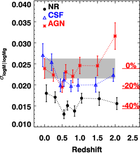
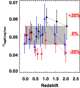
All mass–proxy scaling relations, with the exception of for the nr runs, present a negligible trend with redshift: the scatters at or are consistent within 1 or 1.5 with the scatter. The luminosity-based relations, instead, present a significant variation of the scatter, which decreases with increasing redshift as can be seen in the figure.
The relation always presents the minimum amount of scatter in line with the results from Stanek et al. (2010) and Fabjan et al. (2010). The values are around per cent which are 1.5 times smaller than and a factor of – smaller than the scatter of the two temperatures ( and , respectively). This is not surprising since the value of is consistent with the statistical expectations (Stanek et al., 2010): where the correlation factor between and is not negative.
The increase of 25-50 per cent with redshift of the nr scatter of the scaling relation is most likely generated by the sequence of minor mergers of smaller and colder substructures. Their diffuse gas is efficiently stripped and mixed when the stellar and AGN feedback are present, but it is more resilient to be incorporated to the main cluster ICM in case of the nr simulations (Dolag et al., 2009). The inclusion of the core in the agn runs also increases the scatter of the by 15-20 per cent, while negligible differences (below 3 per cent) are detected for the relation.
The two luminosity-related scaling relations and have the highest intrinsic scatter. They reach 0.2 at and decrease to – at . The largest variation affects the relation. The increase of the scatter in more recent times indicates that the luminosity is sensitive to the entire merger history of the clusters and that the most significant deviations from the global scaling relation originate from recent () massive mergers. A similar trend in the luminosity scatter was recently found by the Weighing the Giants team (Mantz et al., 2016). The variation of the scatter with redshift is an important factor that needs to be considered for cosmological studies. Luckily, the change goes in the direction of reducing, at higher redshift, the Eddington bias caused by the different scattering of objects across the threshold of a flux limited sample (e.g., Stanek et al., 2006; Maughan et al., 2012). Finally, radiative phenomena such as stellar or AGN feedback can also have the effect of diversifying the systems’ luminosity at fixed mass. Indeed, both the csf and agn runs show a 20–30 per cent higher scatter than the nr simulations. The scatter of the agn runs further increases by 20-40 per cent when the core is considered in the computation of the temperature confirming the fragility of this scaling relation since its characterization depends on many factors as already seen in Section 4.
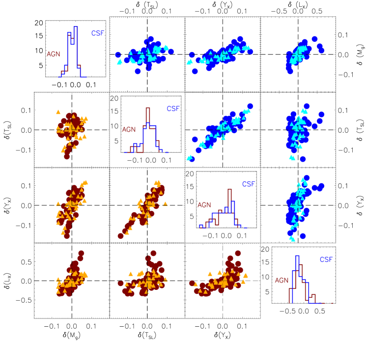
As a second step, we investigated the shape of the deviations of each signal, , from the best-fitting relations at fixed mass and their covariance matrix. In Fig. 10, we report the results for the csf and agn simulations at redshift and , while in Table 4 we also list the coefficients for the nr simulations and for . This analysis allows us to identify the couples of signals with high correlation or anticorrelation. We quantify this measure via the Spearman’s rank coefficient, . In Table 4, we highlight the signal pairs with at a high significance level, i.e. when the null hypothesis probability is less than . These pairs of signals can be jointly used to reduce the mass scatter with respect to the scatter obtained in the individual scaling relations (Stanek et al., 2010; Ettori et al., 2012; Evrard et al., 2014; Wu et al., 2015). The scatter at fixed mass (shown in the diagonal panels) can be accurately described by lognormal distributions (see also Le Brun et al., 2016) at all times.
Regarding the agn physics, we find that all the couples of X-ray quantities present positive correlations at all redshifts with the exception of no correlation found between and at all redshifts and between and at . In addition, we notice that the 0.5 correlation between and at has a 0.2 per cent probability to be obtained by chance, and therefore it is somehow uncertain. The former behaviour is consistent with the already-discussed argument about the different time-scales on the variation of and in reaction to mergers and accretion: since the two quantities increase at subsequent times we do not expect particular correlation. This is particularly true at where no correlation between and is also expected. Indeed, on the one hand, mergers produce an increase of both luminosity and temperature generating a positive correlation between the two deviations. On the other hand, strong AGN bursts, common phenomena at these redshifts, are likely to cause an increase of temperature along with a temporary decrease of luminosity, due to the gas lost as ejected material. This produces a negative correlation. As a confirmation, when the agn are not present the correlation at becomes positive and quite strong, i.e. 0.6 in the nr run and 0.7 in the csf case. The correlation values that we find between and ( and ) at are in good agreement with the value found by Mantz et al. (2016) in a sample containing both relaxed and unrelaxed clusters. In this observational paper, the authors claim a clean separation between the two classes of systems: CC regular systems tend to have higher and than the highly disturbed NCC objects in their sample. In our simulations, we find that the six CC systems that are X-ray regular have, indeed, the largest positive deviation of both quantities.
The parameter shows a strong positive correlation with Spearman’s coefficient with all the parameters considered. Clusters deviate from the mostly due to the changes in their temperature (Rasia et al., 2011) and this is confirmed by the fact that the highest correlation value is that between and . Indeed, is always greater than with the exception of where it still shows a strong correlation with . This result is confirmed even when changing the ICM physics.
We confirm that a combination of the luminosity and temperature () for local clusters as proposed in Ettori (2013) is a good approach to reduce the scatter with respect to the scatters of the individual relations and . In general, the luminosity is well correlated with the other quantities with only few exceptions. A lower level of correlation is found between the luminosity and the temperature in the nr runs and no correlation is detected between the luminosity and the gas mass at higher redshifts. This is most likely related to merging events that significantly boost the luminosity in non-radiative simulations.
The csf and agn runs present similar values of the correlation coefficients beside the mentioned difference at high redshift for the pair and and the associated couple of signals and .
| nr | |||
|---|---|---|---|
| 0.20 (1 ) | 0.50 (3 ) | 0.63 (2 ) | |
| 0.40 (2 ) | 0.61 (1 ) | 0.75 (3 ) | |
| 0.52 (2 ) | 0.42 (8 ) | 0.31 (5 ) | |
| 0.96 (3 ) | 0.98 (0) | 0.96 (2 ) | |
| 0.34 (8 ) | 0.59 (6 ) | 0.59 (7 ) | |
| 0.42 (8 ) | 0.61 (1 ) | 0.57 (1 ) | |
| csf | |||
| 0.33 (9 ) | 0.53 (3 ) | 0.76 (2 ) | |
| 0.72 (4 ) | 0.75 (4 ) | 0.88 (8 ) | |
| 0.73 (4 ) | 0.67 (3 ) | 0.76 (2 ) | |
| 0.87 (2 ) | 0.94 (7 ) | 0.96 (1 ) | |
| 0.40 (2 ) | 0.59 (5 ) | 0.69 (1 ) | |
| 0.65 (2 ) | 0.66 (8 ) | 0.72 (3 ) | |
| agn | |||
| 0.40 (2 ) | 0.24 (4 ) | 0.09 (6 ) | |
| 0.71 (5 ) | 0.68 (2 ) | 0.72 (6 ) | |
| 0.64 (5 ) | 0.62 (3 ) | 0.64 (3 ) | |
| 0.90 (1 ) | 0.84 (3 ) | 0.67 (7 ) | |
| 0.54 (1 ) | 0.52 (2 ) | 0.16 (3 ) | |
| 0.66 (2 ) | 0.72 (6 ) | 0.50 (2 ) |
5.3 The Normalization
The evolution of the normalization is mostly expressed as a power of the factor (see review on scaling-relation evolution by Giodini et al., 2013, and references therein). In other words, the evolution of the normalization is represented as a simple upward or downward shift. In this section, we want to enlighten how this procedure is inaccurate whenever the slope of the considered scaling relation varies with time (Branchesi et al., 2007).
Observationally, we still do not have any indication of evolution of due to the paucity of observed clusters. The situation will improve thanks to the collection of high- data from SPT-3G (Benson et al., 2014) or eROSITA (Giodini et al., 2013). To provide a forecast on the precision that these surveys could reach, there are already ongoing studies that extend local samples by including higher redshift objects. In addition, Bayesian techniques have been developed (see LIRA by Sereno and Ettori 2015a and Sereno 2016 and also Andreon and Hurn 2013). These include a proper treatment for the sample selection (e.g. Sereno and Ettori, 2015a) and the associated selection biases such as the Malmquist and Eddington biases (see Allen et al., 2011, for a discussion). However, the analysis of the data cannot yet be performed in redshift bins, but it, typically, follows two main approaches. Either the slope is computed in a local sample and then fixed to the entire set (e.g. Clerc et al. 2014) or the fit on the scaling relations is simultaneously applied to all objects (e.g. Hilton et al. 2012; Giles et al. 2016).
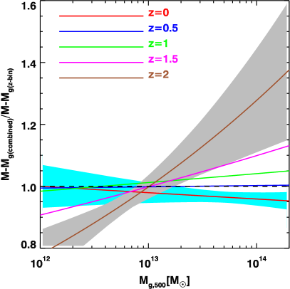
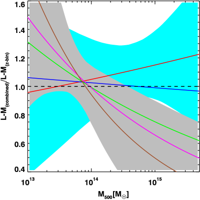
In other words, either method assumes a constant slope. To warn about their application, we focus on the agn and relations because they exhibit the largest slope variation, and therefore they are the best suited to put in evidence a possible misinterpretation of the data. We follow the second observational approach that is the most used and we build a sample that includes the agnsimulated clusters at all redshifts, from to . We fit the combined sample of about 600 objects adopting the equation (11) where the evolution factor , the slope , and the normalization are all free to vary, while is represented by a vector whose length is equal to the number of clusters and each element is computed at the redshift of the corresponding object. The best-fitting parameters and their 1 errors are reported in Table 5.
In Fig.11, we show the differences between this best-fitting relation (of the combined sample) and the relations that we previously presented in Tables 2 and 3 and that were evaluated in single redshift bins. The brown line is for the comparison with the bin and it highlights how much the high- clusters are misrepresented by enforcing a single slope across all redshifts. The most severe differences are present for the relation where an offset affects not only the highest redshift bins but also the local measures. The , whose value is mostly constant up to redshift 1, presents significant changes only at .
For the cases where the slope does not substantially vary with time (in terms of sigma or absolute value) such as , , and , the evolution in their normalization is a well-defined measurement and the usage of a unique fitting function is well justified111111All temperatures are measured after excluding the core region. With the inclusion of the cores, the difference in the normalization, , of the mass-temperature relations is below 2 per cent for both relations ( and ) with the exception of per cent and per cent variation on the normalization of the relation at and , respectively. The differences in the normalization of the relation reach 7 and 10 per cent at and respectively; otherwise they are smaller than 5 per cent. In all circumstances, they are consistent within 1 with the values of Table 3.. In particular, we find that the predicted slope and evolution of both relations are close to the SS expectations (see Table 1) with the slight tendency of less negative evolution than SS in the relation ( versus ) and more positive evolution than SS in the relation ( versus ).
The results for the relation from our agn sample, and , are in line with a positive evolution associated with the slope reported by Giles et al. (2016). This result is, however, in contrast with the measurements of the bolometric luminosity, – erg s-1 of ISCS J1438+3414 at and JKCS041 at by Andreon et al. (2011), of XDCP J0044.0-2033 at by Tozzi et al. (2015), and of IDCS J1426.5+3508 at by Brodwin et al. (2016). If local relations and SS evolution are assumed, all these objects appeared underluminous for their measured temperature ( keV, keV, keV, and keV, respectively) or viceversa hotter for their luminosity. It is difficult to make a significant comparison due to the low number of objects, the large error bars, and the impossibility to evaluate any selection effect. It is, nevertheless, interesting to notice that all these cases are exceptionally massive and almost twice as hot as our most massive clusters at .
6 Comparison with the literature
In this section, we compare our results on the evolution of scaling relations to some previous numerical works after noting that a straightforward comparison is often difficult for the differences in terms of cosmological model, implementation of the ICM physics, and sample selection.
A number of studies have employed simulations to investigate the redshift trend of scaling relations, such as Short et al. (2010), Stanek et al. (2010), Fabjan et al. (2011), Battaglia et al. (2012), Pike et al. (2014), Sembolini et al. (2014), Le Brun et al. (2016), and Barnes et al. (2017).
Our results are consistent with Fabjan et al. (2011) who found no significant redshift trend in the slopes of , , and up to . The samples analysed in that paper were very similar to ours even if we adopted here a more sophisticated implementation of the agn modelling and of the hydrodynamic code.
Planelles et al. (2017) showed that in our sample there is little difference between and . Therefore, the results presented in this paper are also in line with Battaglia et al. (2012), Pike et al. (2014), and Sembolini et al. (2014), who found that the slope remains almost constant up to .
As remarked in Gaspari et al. (2014), AGN feedback is a purely inside-out process affecting primarily the small radii; for massive systems, the binding energy is so large that only the inner core is affected (), thus leaving the integrated properties within essentially unaltered. In the cluster regime, it is thus not surprising that there is no substantial evolution in the global properties. Comparing with Gaspari et al. (2014) models, our dominant AGN feedback appears to be gentle, rather than strong and impulsive as a quasar blast, further limiting major temporal fluctuations.
Further comparing with Pike et al. (2014), we acknowledge an opposite trend with respect to the slope evolution of the relation: while it is decreasing in our case they find a steeper slope at higher redshifts for all physics that they explored including the non-radiative case. This implies that their small mass objects are hotter than ours (at fixed mass); in the paper, the authors suggest that their results might be affected by their sample that was composed by only 30 objects randomly selected to equally populate five logarithm mass bins in the range .
With respect to Le Brun et al. (2016), we already detailed some comparisons regarding the nr case and stressed that we agree with their results. The only exception is the evolution that they show for the relation. In their cosmological box, they also obtain colder groups at with respect to at fixed total mass but they do detect only a small change in the relation slope. This could be due to the position of their most massive systems at that apparently are also colder than their local counterpart. The difference between ours and their results could be ascribed to the hydrodynamical code or even to the way of measuring the spectroscopic-like temperature or a different selection (see below).
It is more interesting, here, to stress similarities and differences between the agn models especially on the relation since all the other relations can be related to this and the already discussed relation. The best-fitting scaling relation proposed by Le Brun et al. (2016) passes through the points of our agn set; however, their conclusions are apparently opposite than ours since they claim an opposite trend for the slope (note that their figure is similar to ours but they consider the relation instead of the one). This seemingly paradox is due to a different choice of sample selection. In that paper, the authors selected all objects with mass above a certain threshold, , which is significantly smaller than our lower limit at any redshift. By including the smallest groups at , the authors are sampling the stable population of clusters together with the population of small groups that exhibit a quickly decline in gas fraction with total mass (see Fig. 7). At , their overall slope is, therefore, shallower than ours, as the smallest-mass systems weight significantly more in number and dominate in the fitting process. Indeed, both their AGN models have while our value of is . At the majority of their objects are characterized by a milder relation because the least massive objects retain more gas than the smallest groups and the most massive objects are not yet formed at those times. On the other hand, in our agn sample we always consider the most massive objects at each redshift, this implies that the mass range selected changes with time. Our sample is mostly on the shallower part of the relation while the opposite is true for the sample.
Concerning the evolution of the normalization, we are consistent with Le Brun et al. (2016) on the positive evolution of the relation, which is caused by the incomplete thermalization of high- clusters. Our result on the positive evolution of the also agrees with the work from Barnes et al. (2017). Finally, our study confirms that there is no significant trend in the intrinsic scatter of the non-luminosity scaling relations as found in most studies in literature (but see Le Brun et al. 2016). For the , Barnes et al. (2017) also found that the scatter in the luminosity decreases towards high redshifts. The similar trend for the , in agreement with our result, is also found in their study, yet less significant.
7 Conclusions
In this paper, we address the evolution of scaling relations in simulated galaxy clusters. Our study is based on an extended set of cosmological hydrodynamic simulations of clusters. The simulations are carried out with the GADGET-3 code with an upgraded implementation of SPH and including both stellar and AGN feedback. We selected all clusters identified within 29 Lagrangian regions above a mass limit whose redshift dependence mimics that of the SPT selection function (Bleem et al., 2015). Our sample of simulated clusters, by construction, is neither volume- nor mass-limited. For this reason, we stress that our results are intended to be read as a discussion of general trends rather than providing as a precise list of fitting parameters for scaling relations and corresponding scatter. We first examine the reliability of our newly performed agn runs by comparing our predictions to those derived from local () and intermediate redshift () observations. Subsequently, we investigate the evolution of six scaling relations: , , , , , and by comparing the agn model with two other parallel runs performed with non-radiative physics or with the inclusion of radiative cooling, star formation, and stellar feedback, but not AGN feedback. We characterize how the features of the scaling relations (namely the slope, intrinsic scatter, and normalization) and the covariance matrix between couples of signals change as a function of redshift. We summarize in the following our main results.
-
•
The scaling relations from simulations at low and intermediate redshifts reproduce reasonably well the observed , , and relations as well as the observed diversity between CC and NCC clusters in the relation. However, our agn model produces lower temperatures than observed resulting in a normalization shift of per cent for the relation in comparison to observations. A shift of 30 per cent is also present in the luminosity mostly due to the sample selection.
-
•
From and , we do not detect any appreciable change of the slopes of the relations with the exclusion of a 4 per cent of the for the nr model and an per cent change of for the nr and csf runs, for the csf and agn simulations and for the agn set).
-
•
At higher redshifts, however, all the relations exhibit some degree of evolution with the only exception being the luminosity relations and the relation of the nr models which remains unchanged. In the agn runs, the gas slope, , at is reduced by per cent with respect to the present-time value. This is caused by the effect of intense high- AGN activity that has more impact on the lowest mass systems, more numerous in the high-redshift bins for the applied SZ-like selection. At , a shallower slope is found also for the relation that declines by per cent with respect to . The evolution of the is not due to the selection, but depends on the fact that the smallest groups have a systematically lower temperature due to their incomplete thermalization at . The decrease of ( per cent) and increase of ( per cent) slopes can be explained by analytically decomposing their slopes in the two contributors: and . Radiative processes reduce the hot gas content by removing the coldest and densest gas to produce stars. The impact is stronger for group-sized objects. This implies that the and relations deviate in different direction from the self-similarity scalings. When combined in the parameter, the SS behaviour is recovered (Kravtsov et al., 2006).
-
•
We do not find any significant redshift trend of the scatter in any of the mass-proxy relations. Consistent with previous theoretical studies, the relation has the smallest scatter. Instead, the scatter of the two luminosity relations, and , is the largest, over the redshift range . The scatter increases with the decrease of redshift enlightening the significant impact on the X-ray luminosity by recent major mergers (Torri et al., 2004). When a merger occurs, the luminosity registers a permanent increase (Rowley et al., 2004). The scatter of all relations can be well described by a lognormal distribution whose widths are mostly constant over the redshift up to .
-
•
The inclusion of the core, defined as the inner sphere within 0.15 , does not significantly influence the best-fitting values of the slopes and normalizations which are consistent within 1 to the respective values obtained in the core-excised sample. The scatter, however, grows by per cent in the relation and by per cent in the relation.
-
•
In the agn run, no correlation is evident between the pair of deviation in and at fixed mass and at all redshift. No correlation is registered also between and at . In all other cases, positive correlations are found with Pearson coefficients always greater than 0.4.
-
•
Regarding the study of the evolution of the normalization, we stress that in situations where the slopes vary with redshift, such as the and in the agn runs, the evolution on the normalization cannot be uniquely established since the trend will depend on the pivotal point used to measure it. Owing to the redshift dependence of slope and normalization of scaling relations, we warn against the fitting with a single relation data for objects distributed over a wide redshift range. On the other hand, we find that the and relations, whose slopes have a milder or no evolution, exhibit a negative and positive evolution of the normalization (respectively, and ) for the redshift range , with values for the evolution parameters in line with recent observational studies and close to the SS predictions.
-
•
Overall, we confirm that the relation evaluated from to is the best suited for cosmological studies for the combination of its properties: in that redshift range, the slope does not vary, the evolution of the normalization can be robustly determined, the scatter is small and constant over time and most importantly the relation is solid, the closest to a SS behaviour, independent from the source of feedback either from star, SN, or AGNs (but see Le Brun et al., 2016, for a different result).
On the basis of our analysis of the intrinsic variations of simulated clusters, we also conclude that pushing the study of the scaling relations to higher redshifts does not seem to be an advantage because the intense AGN activity, peaking at , could have a significant impact and produce deviations from the SS behaviour at redshifts . This cosmic epoch is still almost an unexplored territory where the predictions of higher resolution simulations can help in designing observational strategies for future missions. From an observational perspective, the scaling relations are expected to be calibrated by measuring the mass from weak-lensing analyses (Marrone et al., 2012; Hoekstra et al., 2015; Sereno and Ettori, 2015a; Mantz et al., 2016). However, even if this procedure is not expected to introduce a significant averaged mass bias over a large sample of objects (Meneghetti et al., 2010; Becker and Kravtsov, 2011; Rasia et al., 2012) it will likely enlarge the scatter of the relations (Sereno and Ettori, 2015b) since the lensing mass of single clusters can be both underestimated and overestimated by a considerable amount. Finally, attention will have to be devoted to clusters close to the flux limit threshold (Nord et al., 2008). Certainly, more efforts will need to be dedicated to reducing the uncertainties on the mass calibration down to the few per cent level.
ACKNOWLEDGEMENTS
We are greatly indebted to Volker Springel for giving us access to the developer version of the GADGET3 code; to the entire MUSIC team for sending their simulated data, and to Dolag’s group who built and updates the Magneticum Pathfinder Webportal. We would like to thank Gustavo Yepes, Stefano Ettori, and Mauro Sereno for providing useful discussions and comments. We acknowledge support from the following: the Hungarian Academy of Sciences for the grant Lendület LP2016-11 (NT); PIIF-GA- 2013-627474 (ER); NSF AST-1210973 (ER); ASI Grant 2016-24-H.0 (PM); the Spanish Ministerio de Economía y Competitividad (MINECO) grants AYA2013-48226-C3-2-P and AYA2016-77237-C3-3-P (S.P.); the Generalitat Valenciana, grant GVACOMP2015-227 (SP); the Slovenian Research Agency, research core funding No. P1-0188 (DF); the DFG Cluster of Excellence “Origin and Structure of the Universe” (AMB); the DFG Research Unit 1254 “ Magnetisation of interstellar and intergalactic medium” (AMB); CONICET, FonCyT and SeCyT-UNC, Argentina (CRF); NASA through Einstein PostDoctoral Fellowship Award Number PF5-160137 and Chandra GO7-18121X issued by the Chandra X-ray Observatory Center, which is operated by the SAO for and on behalf of NASA under contract NAS8-03060 (MG). This work is also supported by the PRIN-MIUR 201278X4FL “Evolution of cosmic baryons” funded by the Italian Ministry of Research, by the PRIN-INAF 2012 grant “The Universe in a Box: Multi-scale Simulations of Cosmic Structures”, by the INDARK INFN grant, by the “Consorzio per la Fisica di Trieste”. Simulations were performed using Flux HCP Cluster at the University of Michigan and the Galileo Machine at CINECA with CPU time assigned through ISCRA proposals and an agreement with the University of Trieste. Data, post-processing, and storage have been done on the CINECA facility PICO, granted to us thanks to our expression of interest.
References
- Akritas and Bershady (1996) Akritas M.G., Bershady M.A., 1996, ApJ, 470, 706
- Allen et al. (2011) Allen S.W., Evrard A.E., Mantz A.B., 2011, ARA&A, 49, 409
- Andreon and Hurn (2013) Andreon S., Hurn M., 2013, Statistical Analysis and Data Mining: The ASA Data Science Journal, Vol. 9, Issue 1, p. 15-33, 6, 15
- Andreon et al. (2011) Andreon S., Trinchieri G., Pizzolato F., 2011, MNRAS, 412, 2391
- Ascaso et al. (2017) Ascaso B., Mei S., Bartlett J.G., Benítez N., 2017, MNRAS, 464, 2270
- Bahé et al. (2012) Bahé Y.M., McCarthy I.G., King L.J., 2012, MNRAS, 421, 1073
- Barnes et al. (2017) Barnes D.J., Kay S.T., Henson M.A., McCarthy I.G., Schaye J., Jenkins A., 2017, MNRAS, 465, 213
- Battaglia et al. (2012) Battaglia N., Bond J.R., Pfrommer C., Sievers J.L., 2012, ApJ, 758, 74
- Battaglia et al. (2013) Battaglia N., Bond J.R., Pfrommer C., Sievers J.L., 2013, ApJ, 777, 123
- Beck et al. (2016) Beck A.M., et al., 2016, MNRAS, 455, 2110
- Becker and Kravtsov (2011) Becker M.R., Kravtsov A.V., 2011, ApJ, 740, 25
- Benson et al. (2014) Benson B.A., et al., 2014, in Millimeter, Submillimeter, and Far-Infrared Detectors and Instrumentation for Astronomy VII, vol. 9153 of Proc. SPIE, p. 91531P
- Biffi et al. (2014) Biffi V., Sembolini F., De Petris M., Valdarnini R., Yepes G., Gottlöber S., 2014, MNRAS, 439, 588
- Biffi et al. (2016) Biffi V., et al., 2016, ApJ, 827, 112
- Biffi et al. (2017) Biffi V., et al., 2017, MNRAS, 468, 531
- Bleem et al. (2015) Bleem L.E., et al., 2015, ApJS, 216, 27
- Bonafede et al. (2011) Bonafede A., Dolag K., Stasyszyn F., Murante G., Borgani S., 2011, MNRAS, 418, 2234
- Borgani and Guzzo (2001) Borgani S., Guzzo L., 2001, Nature, 409, 39
- Borgani and Kravtsov (2011) Borgani S., Kravtsov A., 2011, Advanced Science Letters, 4, 204
- Borm et al. (2014) Borm K., Reiprich T.H., Mohammed I., Lovisari L., 2014, A&A, 567, A65
- Branchesi et al. (2007) Branchesi M., Gioia I.M., Fanti C., Fanti R., 2007, A&A, 472, 739
- Brodwin et al. (2016) Brodwin M., McDonald M., Gonzalez A.H., Stanford S.A., Eisenhardt P.R., Stern D., Zeimann G.R., 2016, ApJ, 817, 122
- Bryan and Norman (1998) Bryan G.L., Norman M.L., 1998, ApJ, 495, 80
- Clerc et al. (2014) Clerc N., et al., 2014, MNRAS, 444, 2723
- Dai et al. (2010) Dai X., Bregman J.N., Kochanek C.S., Rasia E., 2010, ApJ, 719, 119
- Dolag et al. (2009) Dolag K., Borgani S., Murante G., Springel V., 2009, MNRAS, 399, 497
- Dolag et al. (2016) Dolag K., Komatsu E., Sunyaev R., 2016, MNRAS, 463, 1797
- Eckert et al. (2016) Eckert D., et al., 2016, A&A, 592, A12
- Erben et al. (2013) Erben T., et al., 2013, MNRAS, 433, 2545
- Ettori (2013) Ettori S., 2013, MNRAS, 435, 1265
- Ettori (2015) Ettori S., 2015, MNRAS, 446, 2629
- Ettori et al. (2012) Ettori S., Rasia E., Fabjan D., Borgani S., Dolag K., 2012, MNRAS, 420, 2058
- Evrard et al. (2014) Evrard A.E., Arnault P., Huterer D., Farahi A., 2014, MNRAS, 441, 3562
- Fabian et al. (1994) Fabian A.C., Crawford C.S., Edge A.C., Mushotzky R.F., 1994, MNRAS, 267, 779
- Fabjan et al. (2010) Fabjan D., Borgani S., Tornatore L., Saro A., Murante G., Dolag K., 2010, MNRAS, 401, 1670
- Fabjan et al. (2011) Fabjan D., Borgani S., Rasia E., Bonafede A., Dolag K., Murante G., Tornatore L., 2011, MNRAS, 416, 801
- Gaspari and Sa̧dowski (2017) Gaspari M., Sa̧dowski A., 2017, ApJ, 837, 149
- Gaspari et al. (2014) Gaspari M., Brighenti F., Temi P., Ettori S., 2014, ApJL, 783, L10
- Gaspari et al. (2017) Gaspari M., Temi P., Brighenti F., 2017, MNRAS, 466, 677
- Giles et al. (2016) Giles P.A., et al., 2016, A&A, 592, A3
- Giles et al. (2017) Giles P.A., et al., 2017, MNRAS, 465, 858
- Giodini et al. (2013) Giodini S., Lovisari L., Pointecouteau E., Ettori S., Reiprich T.H., Hoekstra H., 2013, Space Sci. Rev., 177, 247
- Haardt and Madau (2001) Haardt F., Madau P., 2001, in D.M. Neumann, J.T.V. Tran, eds., Clusters of Galaxies and the High Redshift Universe Observed in X-rays, p. 64
- Hahn et al. (2017) Hahn O., Martizzi D., Wu H.Y., Evrard A.E., Teyssier R., Wechsler R.H., 2017, MNRAS, 470, 166
- Heymans et al. (2012) Heymans C., et al., 2012, MNRAS, 427, 146
- Hilton et al. (2012) Hilton M., et al., 2012, MNRAS, 424, 2086
- Hoekstra et al. (2015) Hoekstra H., Herbonnet R., Muzzin A., Babul A., Mahdavi A., Viola M., Cacciato M., 2015, MNRAS, 449, 685
- Hudson et al. (2010) Hudson D.S., Mittal R., Reiprich T.H., Nulsen P.E.J., Andernach H., Sarazin C.L., 2010, A&A, 513, A37
- Isobe et al. (1990) Isobe T., Feigelson E.D., Akritas M.G., Babu G.J., 1990, ApJ, 364, 104
- Ivezic et al. (2008) Ivezic Z., Tyson J.A., et al. for the LSST Collaboration, 2008, preprint, (arXiv:0805.2366)
- Kaiser (1986) Kaiser N., 1986, MNRAS, 222, 323
- Kay et al. (2012) Kay S.T., Peel M.W., Short C.J., Thomas P.A., Young O.E., Battye R.A., Liddle A.R., Pearce F.R., 2012, MNRAS, 422, 1999
- Kelly (2007) Kelly B.C., 2007, ApJ, 665, 1489
- Khatri and Gaspari (2016) Khatri R., Gaspari M., 2016, MNRAS, 463, 655
- Komatsu et al. (2011) Komatsu E., et al., 2011, ApJS, 192, 18
- Kravtsov et al. (2006) Kravtsov A.V., Vikhlinin A., Nagai D., 2006, ApJ, 650, 128
- Laureijs et al. (2011) Laureijs R., et al., 2011, preprint, (arXiv:1110.3193)
- Le Brun et al. (2014) Le Brun A.M.C., McCarthy I.G., Schaye J., Ponman T.J., 2014, MNRAS, 441, 1270
- Le Brun et al. (2016) Le Brun A.M.C., McCarthy I.G., Schaye J., Ponman T.J., 2016, MNRAS
- Lieu et al. (2016) Lieu M., et al., 2016, A&A, 592, A4
- Mahdavi et al. (2013) Mahdavi A., Hoekstra H., Babul A., Bildfell C., Jeltema T., Henry J.P., 2013, ApJ, 767, 116
- Mahdavi et al. (2014) Mahdavi A., Hoekstra H., Babul A., Bildfell C., Jeltema T., Henry J.P., 2014, ApJ, 794, 175
- Mantz et al. (2016) Mantz A.B., et al., 2016, MNRAS, 463, 3582
- Markevitch (1998) Markevitch M., 1998, ApJ, 504, 27
- Marrone et al. (2012) Marrone D.P., et al., 2012, ApJ, 754, 119
- Martizzi et al. (2014) Martizzi D., Mohammed I., Teyssier R., Moore B., 2014, MNRAS, 440, 2290
- Maughan (2014) Maughan B.J., 2014, MNRAS, 437, 1171
- Maughan et al. (2012) Maughan B.J., Giles P.A., Randall S.W., Jones C., Forman W.R., 2012, MNRAS, 421, 1583
- Maughan et al. (2016) Maughan B.J., Giles P.A., Rines K.J., Diaferio A., Geller M.J., Van Der Pyl N., Bonamente M., 2016, MNRAS, 461, 4182
- Mazzotta et al. (2004) Mazzotta P., Rasia E., Moscardini L., Tormen G., 2004, MNRAS, 354, 10
- McCarthy et al. (2011) McCarthy I.G., Schaye J., Bower R.G., Ponman T.J., Booth C.M., Dalla Vecchia C., Springel V., 2011, MNRAS, 412, 1965
- McDonald et al. (2013) McDonald M., et al., 2013, ApJ, 774, 23
- McNamara and Nulsen (2012) McNamara B.R., Nulsen P.E.J., 2012, New Journal of Physics, 14, 055023
- Menanteau et al. (2013) Menanteau F., et al., 2013, ApJ, 765, 67
- Meneghetti et al. (2010) Meneghetti M., Rasia E., Merten J., Bellagamba F., Ettori S., Mazzotta P., Dolag K., Marri S., 2010, A&A, 514, A93
- Merloni et al. (2012) Merloni A., et al., 2012, preprint, (arXiv:1209.3114)
- Muldrew et al. (2015) Muldrew S.I., Hatch N.A., Cooke E.A., 2015, MNRAS, 452, 2528
- Murray et al. (2013) Murray S.G., Power C., Robotham A.S.G., 2013, Astronomy and Computing, 3, 23
- Nagai et al. (2007a) Nagai D., Kravtsov A.V., Vikhlinin A., 2007a, ApJ, 668, 1
- Nagai et al. (2007b) Nagai D., Vikhlinin A., Kravtsov A.V., 2007b, ApJ, 655, 98
- Nord et al. (2008) Nord B., Stanek R., Rasia E., Evrard A.E., 2008, MNRAS, 383, L10
- Pierre et al. (2016) Pierre M., et al., 2016, A&A, 592, A1
- Pike et al. (2014) Pike S.R., Kay S.T., Newton R.D.A., Thomas P.A., Jenkins A., 2014, MNRAS, 445, 1774
- Planelles et al. (2013) Planelles S., Borgani S., Dolag K., Ettori S., Fabjan D., Murante G., Tornatore L., 2013, MNRAS, 431, 1487
- Planelles et al. (2014) Planelles S., Borgani S., Fabjan D., Killedar M., Murante G., Granato G.L., Ragone-Figueroa C., Dolag K., 2014, MNRAS, 438, 195
- Planelles et al. (2015) Planelles S., Schleicher D.R.G., Bykov A.M., 2015, Space Sci. Rev., 188, 93
- Planelles et al. (2017) Planelles S., et al., 2017, MNRAS, 467, 3827
- Poole et al. (2007) Poole G.B., Babul A., McCarthy I.G., Fardal M.A., Bildfell C.J., Quinn T., Mahdavi A., 2007, MNRAS, 380, 437
- Puchwein et al. (2008) Puchwein E., Sijacki D., Springel V., 2008, ApJL, 687, L53
- Ragagnin et al. (2017) Ragagnin A., Dolag K., Biffi V., Cadolle Bel M., Hammer N.J., Krukau A., Petkova M., Steinborn D., 2017, Astronomy and Computing, 20, 52
- Rasia et al. (2004) Rasia E., Tormen G., Moscardini L., 2004, MNRAS, 351, 237
- Rasia et al. (2011) Rasia E., Mazzotta P., Evrard A., Markevitch M., Dolag K., Meneghetti M., 2011, ApJ, 729, 45
- Rasia et al. (2012) Rasia E., et al., 2012, New Journal of Physics, 14, 055018
- Rasia et al. (2015) Rasia E., et al., 2015, ApJL, 813, L17
- Reichert et al. (2011) Reichert A., Böhringer H., Fassbender R., Mühlegger M., 2011, A&A, 535, A4
- Rowley et al. (2004) Rowley D.R., Thomas P.A., Kay S.T., 2004, MNRAS, 352, 508
- Sartoris et al. (2016) Sartoris B., et al., 2016, MNRAS, 459, 1764
- Sembolini et al. (2013) Sembolini F., Yepes G., De Petris M., Gottlöber S., Lamagna L., Comis B., 2013, MNRAS, 429, 323
- Sembolini et al. (2014) Sembolini F., De Petris M., Yepes G., Foschi E., Lamagna L., Gottlöber S., 2014, MNRAS, 440, 3520
- Sembolini et al. (2016a) Sembolini F., et al., 2016a, MNRAS, 457, 4063
- Sembolini et al. (2016b) Sembolini F., et al., 2016b, MNRAS, 459, 2973
- Sereno (2016) Sereno M., 2016, MNRAS, 455, 2149
- Sereno and Ettori (2015a) Sereno M., Ettori S., 2015a, MNRAS, 450, 3675
- Sereno and Ettori (2015b) Sereno M., Ettori S., 2015b, MNRAS, 450, 3633
- Short and Thomas (2009) Short C.J., Thomas P.A., 2009, ApJ, 704, 915
- Short et al. (2010) Short C.J., Thomas P.A., Young O.E., Pearce F.R., Jenkins A., Muanwong O., 2010, MNRAS, 408, 2213
- Simionescu et al. (2017) Simionescu A., Werner N., Mantz A., Allen S.W., Urban O., 2017, MNRAS, 469, 1476
- Smith et al. (2001) Smith R.K., Brickhouse N.S., Liedahl D.A., Raymond J.C., 2001, ApJL, 556, L91
- Springel (2005) Springel V., 2005, MNRAS, 364, 1105
- Springel and Hernquist (2003) Springel V., Hernquist L., 2003, MNRAS, 339, 289
- Springel et al. (2005) Springel V., Di Matteo T., Hernquist L., 2005, MNRAS, 361, 776
- Stanek et al. (2006) Stanek R., Evrard A.E., Böhringer H., Schuecker P., Nord B., 2006, ApJ, 648, 956
- Stanek et al. (2010) Stanek R., Rasia E., Evrard A.E., Pearce F., Gazzola L., 2010, ApJ, 715, 1508
- Steinborn et al. (2015) Steinborn L.K., Dolag K., Hirschmann M., Prieto M.A., Remus R.S., 2015, MNRAS, 448, 1504
- Sun et al. (2009) Sun M., Voit G.M., Donahue M., Jones C., Forman W., Vikhlinin A., 2009, ApJ, 693, 1142
- Takey et al. (2013) Takey A., Schwope A., Lamer G., 2013, A&A, 558, A75
- Tormen et al. (1997) Tormen G., Bouchet F.R., White S.D.M., 1997, MNRAS, 286, 865
- Tornatore et al. (2007) Tornatore L., Borgani S., Dolag K., Matteucci F., 2007, MNRAS, 382, 1050
- Torri et al. (2004) Torri E., Meneghetti M., Bartelmann M., Moscardini L., Rasia E., Tormen G., 2004, MNRAS, 349, 476
- Tozzi et al. (2015) Tozzi P., et al., 2015, ApJ, 799, 93
- Vikhlinin (2006) Vikhlinin A., 2006, ApJ, 640, 710
- Vikhlinin et al. (2009) Vikhlinin A., et al., 2009, ApJ, 692, 1033
- Villaescusa-Navarro et al. (2016) Villaescusa-Navarro F., et al., 2016, MNRAS, 456, 3553
- Voit (2005) Voit G.M., 2005, Reviews of Modern Physics, 77, 207
- von der Linden et al. (2014) von der Linden A., et al., 2014, MNRAS, 443, 1973
- Watson et al. (2013) Watson W.A., Iliev I.T., D’Aloisio A., Knebe A., Shapiro P.R., Yepes G., 2013, MNRAS, 433, 1230
- Weinberg et al. (2013) Weinberg D.H., Mortonson M.J., Eisenstein D.J., Hirata C., Riess A.G., Rozo E., 2013, Phys. Rep., 530, 87
- Wiersma et al. (2009) Wiersma R.P.C., Schaye J., Theuns T., Dalla Vecchia C., Tornatore L., 2009, MNRAS, 399, 574
- Wu et al. (2015) Wu H.Y., Evrard A.E., Hahn O., Martizzi D., Teyssier R., Wechsler R.H., 2015, MNRAS, 452, 1982
Appendix A Decomposition of the slopes of composite signals
In this section we derive the features of , , and based on the two fundamental relations: and :
| (17) |
| (18) |
The relation. By definition the is the product of gas mass and temperature, and thus
| (19) |
From equations (A1)-(A3), one deduces
| (20) |
Writing in general form
| (21) |
the slope and power of evolution of the are given by
| (22) |
| (23) |
The relation. The general form of is given by
| (24) |
Recalling that is related to the total mass and temperature via equation (8)
| (25) | |||||
In the last derivation we use equation (A1) to rewrite in terms of . In turn, by substituting in terms of via equation (A2) one obtains
| (26) | |||||
By comparing equation (A10) to equation (A8) one deduces
| (27) |
| (28) |
The relation. We define the general form of as
| (29) |
In equation (A9), we rewrite in term of via equation (A2) and obtain
| (30) |
From the last equation we can derive the slope and evolution of the relation given as
| (31) |
| (32) |