Lifted Region-Based Belief Propagation

Abstract

Due to the intractable nature of exact lifted inference, research has recently focused on the discovery of accurate and efficient approximate inference algorithms in Statistical Relational Models (SRMs), such as Lifted First-Order Belief Propagation. FOBP simulates propositional factor graph belief propagation without constructing the ground factor graph by identifying and lifting over redundant message computations. In this work, we propose a generalization of FOBP called Lifted Generalized Belief Propagation, in which both the region structure and the message structure can be lifted. This approach allows more of the inference to be performed intra-region (in the exact inference step of BP), thereby allowing simulation of propagation on a graph structure with larger region scopes and fewer edges, while still maintaining tractability. We demonstrate that the resulting algorithm converges in fewer iterations to more accurate results on a variety of SRMs.

Introduction

Statistical relational models (SRMs) have grown in popularity because of their ability to represent a rich relational structure with underlying uncertainty. However, the discovery of general-purpose, fast, and accurate inference algorithms in SRMs has remained elusive. Exact lifted inference techniques harness symmetries in the relational structure of SRMs in order to perform efficient inference, but the involved structure of many real-world domain problems disallow the use of efficient exact inference. Recent research has focused on discovery of accurate approximate inference algorithms, such as Lifted Sampling techniques (?; ?) and Lifted Belief Propagation (?; ?; ?).

For example, given a model, Lifted First-Order Belief Propagation (FOBP) (?) simulates loopy belief propagation on the corresponding propositional factor graph induced by identifying messages that are provably identical at each iteration of LBP and ’lifting’ over them, namely computing them only once and replacing products of identical messages by their appropriate powers (e.g., $\prod_{i=1}^{n}\phi=(\phi)^{n}$). The resulting approximation is provably equivalent to the approximation obtained by running propositional LBP but with a potentially lower time and space complexity. While FOBP often yields good results in practice, it suffers from the same drawback as LBP; namely, the accuracy of its approximations depends on the structure of the underlying factor graph. In general, loopier factor graphs yield poorer approximations. This problem is exacerbated in relational models, where the underlying factor graphs tend to be densely connected.

Researchers have proposed a myriad of LBP variants in order to improve the algorithm’s efficacy. One significant line of research has focused on the observation that factor graphs with fewer loops tend to converge more often and to better approximations (for example, on tree-structured factor graphs BP yields exact answers, and that factor graphs with a single loop always converge, although to possibly erroneous approximations (?)). One way to reduce the number of loops is to reduce the number of edges in the message passing structure; therefore a large-class of algorithms specify some generalization of the factor graph structure that allows factors to be clustered together into regions (e.g. (?; ?)). These algorithms allow for the exchange of cheap, approximate inference (i.e. inter-cluster message passing) for expensive, exact inference (i.e. intra-cluster variable elimination). The resulting schemes allow the user to trade algorithmic complexity for more likely convergence and better approximation accuracy.

We propose a generalized belief propagation scheme for SRMs. The scheme employs exact lifted inference rules to compactly encode the potential structure at each region, thus admitting regions with much larger factor and variable sets than possible with propositional schemes. Our scheme harnesses the symmetric nature of relational models in order to pass joint messages over groups of exchangeable variables. In conjunction as well as offloading the approximate, inter-cluster inference step of LBP (message passing) into the exact, intra-cluster step of LBP (sum-product inference) whenever efficient, allowing the simulation of propagation on region graphs with larger region scopes and fewer edges while still maintaining tractability. We demonstrate that the resulting algorithm converges in fewer iterations to more accurate results on a variety of relational models.

Background

Markov Logic

Statistical relational modeling languages combine graphical models with elements of first-order logic, by defining template features that apply to whole classes of objects at once. One such simple and powerful language is Markov logic (?). We formally define a Markov Logic Network as follows:

• A Markov Logic Network (MLN) $M$ is a pair $\langle F,C\rangle$, in which $F$ is a set of weighted clauses, $\{\langle f_{1},w_{1}\rangle,\ldots,\langle f_{n},w_{n}\rangle\}$, where $f_{i}$ is a first order clause (all logical variables in $f_{i}$ are assumed to be universally quantified and standardized apart for simplicity) and $w_{i}\in\mathbb{R}$ is its corresponding weight, and $C$ is a list of constraints over the logical variables of each $f_{i}$. We adopt the constraint language similar to that presented in (?), in which each constraint is either a domain constraint (i.e. $x\in\tau_{i}$, where $\tau_{i}$ is an ordered set of constants or objects $\{c_{1},\ldots,c_{n}\}$ called the domain of $x$), an equality constraint (i.e. $x=y$), or an inequality constraint (i.e. $x\neq y$).

Let $V=lvars(F)$, the set of all logical variables in $F$. Then the tuple $\langle V,C\rangle$ defines a constraint satisfaction problem. Let $\Theta$ be the set of solutions to $\langle V,C\rangle$. Then $\{R\theta\mid R\in F,\theta\in\Theta\}$ is the set of ground atoms of $M$, and $\{f_{i}\theta\mid f_{i}\in F,\theta\in\Theta\}$ is the set of ground formulas of $M$. For example, the first-order clause $\forall x\forall y\;S(x)\vee\neg T(y)$ given the constraint $x\neq y$ and constants $\{a_{1},a_{2}\}$ yields the following two ground features: $S(a_{1})\vee\neg T(a_{2})$ and $S(a_{2})\vee\neg T(a_{1})$. Every MLN defines a Markov network with one node per ground atom and one feature per ground formula. The weight of a feature is the weight of the first-order clause that originated it. The probability of a state $x$ in such a network is given by $P(x)=\frac{1}{Z}\exp(\sum_{i}w_{i}g_{i}(x))$, where $w_{i}$ is the weight of the $i$-th (ground) feature, $g_{i}(x)=1$ if the $i$-th feature is true in $x$, and $0$ otherwise.

Generalized Belief Propagation

Loopy Belief propagation (?) is an approximate inference procedure for graphical models. Given a model, the algorithm operates by iteratively passing messages between adjacent nodes on the corresponding factor graph until marginal beliefs converge for all variables in the model (or a bound on the number of iterations is reached). Generalized Belief Propagation (?) is a generalization of the LBP algorithm that operates on an underlying graph structure called a region graph.

• Given a PGM $P=\langle X,F\rangle$, where $X$ is a set of random variables and $F$ is a set of factors, a region graph is a labeled, directed graph $G=(V,E,L)$, in which each vertex $v\in V$ (corresponding to a region) is labeled with a subset of $X$ and a subset of $F$. We denote the label of vertex $v$ by $l(v)\in L$. A directed edge $e\in E$ may exist pointing from vertex $v_{p}$ to vertex $v_{c}$ if $l(v_{c})$ is a subset of $l(v_{p})$.

In the canonical message passing formulation (called the parent-to-child algorithm), each region $R$ has a belief $b_{R}(x_{R})$ given by:

$$b_{R}(x_{R})=\prod_{a\in a_{R}}f_{a}(x_{a})\left(\prod_{P\in P(R)}m_{P\rightarrow R}(x_{R})\right)\\ \left(\prod_{D\in D(R)}\prod_{P^{\prime}\in P(D)\setminus\mathcal{E}(R)}m_{P^{\prime}\rightarrow D}(x_{D})\right)$$ (1)

Here $P(R)$ is the set of regions that are parents to region $R$, $D(R)$ is the set of all regions that are descendants of region $R$, $\mathcal{E}(R)=R\cup D(R)$ is the set of all regions that are descendants of $R$ and also region $R$ itself, and $P(D)\setminus\mathcal{E}(R)$ is the set of all regions that are parents of region $D$ except for region $R$ itself or those regions that are also descendants of region $R$. The message-update rule is derived by insisting on equality between the joint distributions between adjacent nodes.

Exchangeable Normal Form

Our proposed Lifted Generalized Belief Propagation (LGBP) algorithm relies on the exchangeable nature of the ground formulas associated with a lifted formula in order to send and receive compact messages over large groups of variables. As such, the algorithm requires that the input MLN be preprocessed into a format that facilitates construction of these messages. We call it exchangeable normal form, defined formally below:

• Let MLN $M=\langle F,C\rangle.$ Let $G_{i}$ be the set of ground formulas associated with formula $f_{i}\in F$. $M$ is said to be in exchangeable normal form if and only if $\forall g_{j},g_{k}\in G_{i}$, the joint distribution $P(Vars(g_{j}))$ equals $P(Vars(g_{k}))$ subject to renaming of the random variables, where $Vars(g_{i})$ is the set of propositional (random) variables in $g_{i}$.

• Consider the MLN $M$ consisting of the single formula:

  $$\langle S(x)\vee\neg S(y)\vee\neg F(x,y),w\rangle\{x,y\in\{a_{1},a_{2}\}\}$$

  $M$ is not in exchangeable normal form. The ground formulas in which $x=y$ can have a different distribution than those in which $x\neq y$. To see why, note that if $x=y$ the ground formula becomes a tautology, whereas if $x\neq y$, it does not. However, we can rewrite the formula of $M$ as $M^{\prime}$, in which the formula is shattered into two formulas with associated constraints.

  $$\langle S(x_{1})\vee\neg S(y_{1})\vee\neg F_{x=y}(x_{1},y_{1}),w\rangle$$

  $$\langle S(x_{2})\vee\neg S(y_{2})\vee\neg F_{x\neq y}(x_{2},y_{2}),w\rangle$$

  $$\{x_{1},x_{2},y_{1},y_{2}\in\{a_{1},a_{2}\},x_{1}=y_{1},x_{2}\neq y_{2}\}$$

  $M^{\prime}$ is in exchangeable normal form.

Lifted Inference

Lifted inference is a collection of techniques that exploit the symmetries in graphical models in order to efficiently compute the partition function (via sum-product based inference). Since its introduction (?), researchers have developed a variety of algorithms for performing exact lifted inference (e.g. (?; ?; ?; ?)). Each of these algorithms rely on a handful of lifting rules that dictate when and how to perform inference efficiently. We discuss two rules that are common to popular algorithms.

• (Lifted Sum.) Given a model $M$ with set of exchangeable random variables $X$, where $\lvert X\rvert=n,Z(M)=\sum_{k=0}^{n}{n\choose k}Z(M\lvert\{x_{1},\ldots,x_{k}\}=T,\{x_{k+1},\ldots,x_{n}\}=F)$

• (Lifted Product.) Given a model $M$ that is decomposable into a collection of independent subproblems $\{{\bf M_{1}},\ldots,{\bf M_{n}}\},$ where each subproblem $M_{i}\in{\bf M_{i}}$ is identical, the partition function of $M,Z(M)=\prod_{i=1}^{n}Z(M_{i})^{\lvert{\bf M_{i}}\rvert}$

Exact lifted inference can be applied to any PGM, but it is particularly effective on templated models (such as MLNs) because (1) sets of independent and identical subproblems and (2) sets of exchangeable random variables can often be readily identified from the template structure. We can view the heuristic decisions as to which lifting rules to apply during execution on model $M$ as a partially ordered set. Further, because unordered pairs of elements represent the roots of independent subproblems, the ordering defines a rooted tree, which we call a lifted factorization.

• A lifted factorization for model $M$ is a rooted, labeled tree $E_{M}=\langle V,E\rangle$, in which:

  1. each vertex $v\in V$ is labeled by a $k$-arity predicate $R(i_{1},\ldots,i_{k}),$ where $\{i_{1},\ldots,i_{k}\}\in\{C,D,G\}$, where:

     1. $i_{j}=C$ indicates that the inference algorithm performs the lifted sum operation over the set of exchangeable random variables represented by $R\theta,$ where $\theta=\{x_{1}=c_{1},x_{k}=c_{k},x_{j}\in D_{x_{j}}\}$.

     2. $i_{j}=D$ indicates that the inference algorithm has decomposed over the set of logical variables appearing at position $j$ in predicate $R$ in $M$ (lifted product rule), and

     3. $i_{j}=G$ indicates that the inference algorithm grounds the set of logical variables appearing at position $j$ in predicate $R$ in $M$.

  2. each edge $e\in E$ is labeled by a (possibly empty) set of logical variables $X$ that decompose the subproblem represented by the tree below into identical subproblems.

Figure 1: Two lifted factorizations for the MLN $R(x)\vee S(y)$ with $\{x\in\{1,2\},y\in\{1,2\}\}$, and their lifted inference representations.

A lifted factorization is valid for model $M$ if the application of each inference rule over the subtree rooted at each node is valid (i.e. meets the preconditions of the rule). All valid lifted factorizations for $M$ are correct in that they return the same partition function. However, each choice encodes a different factorization of the (unnormalized) joint probability distribution. Therefore, some lifted factorizations yield more efficient inference than others. Further, the joint marginal probability distribution of a set of random variables is only (efficiently) available if they occur on the same path from root to leaf. Hence, different factorizations admit efficient access to the joint distribution over different sets of random variables.

• Consider the MLN $M=R(x)\vee S(y)$ with $\{x\in\{1,2\},y\in\{1,2\}\}$. Figure 1 (left) shows a possible lifted factorization for $M$, which applies the Lifted Sum Rule to $R$, then applies the Lifted Product Rule to $\{y\}$, then applies the Lifted Sum Rule to a single grounding of $S$. This lifted factorization yields a search space with $6$ leaves, which admits efficient access to the joint marginal distribution over sets $\{R(1),R(2),S(1)\}$ or $\{R(1),R(2),S(2)\}$ (which are equivalent up to a renaming of $S$), but not over the full joint distribution $\{R(1),R(2),S(1),S(2)\}$. Figure 1 (right) does not apply the lifted product rule, yielding a (larger) lifted search space with $9$ leaves, which admits efficient access to the joint marginal distribution over all subsets of the random variables $\{R(1),R(2),S(1),S(2)\}$.

• Given a MLN $M$ with ground atoms $A_{M}$ and an associated valid lifted factorization $E$, define $JD(M,E)=\{V\mid V\subseteq A_{M},P(V)$ can be accessed efficiently under lifted factorization $E\}$.

Lifted Generalized Belief Propagation

Figure 2: Three types of simulated region graphs for the model $R(x)\vee S(y),R(x)\vee T(z),$ with domain sizes $\Delta_{x}=\Delta_{y}=\Delta_{z}=\{1\ldots 10\}$. Light grey rectangles represent ground factors. Light grey circles represent ground atoms. Dark grey rectangle represent lifted factors. Dark grey circles represent lifted atoms.

Given a model $M$, FOBP (?) takes advantage of redundant messages in order to simulate the message passing procedure on the factor graph of $M$ without explicitly constructing the factor graph. We refer to this kind of lifting operation as message-based lifting. Our new scheme, Lifted Generalized Belief Propagation (LGBP) improves on this algorithm in two ways. First, LGBP harnesses lifted inference rules in order to compactly represent large sets of factors and variables within a cluster whenever it is efficient. We refer to this kind of lifting operation as region-based lifting. Second, wherever it is possible LGBP uses a lifted representation of the messages themselves; this representation allows message passing over the joint distribution of collections of exchangeable atoms rather than over multiple copies of singleton atoms.

• Figure 2 depicts three variants of simulated region graphs for the MLN $R(x)\vee S(y),R(x)\vee T(z)$, with constraint set $x\in\{a_{1},\ldots a_{10}\},y\in\{b_{1},\ldots b_{10}\},z\in\{c_{1},\ldots,c_{10}\}$. Figure 2 (left) depicts the propositional factor graph (which FOBP simulates). Figure 2 (middle) depicts the region graph in which all factors are lifted (via region-based lifting), but messages are still passed over ground variables (via message-based lifting). Figure 2 (right) depicts a region graph in which the factors and messages are lifted (i.e. all groundings of each formula in the MLN appear within the same cluster, and the clusters communicate through a single message containing the joint distribution over $\{R(1)\ldots R(10)\}$). In this case the simulated region graph is a tree; hence, inference is exact.

In particular, if the complexity of propositional region graph BP is $O(n\exp(w))$ where $n$ is the number of messages and $w$ is the maximum number of random variables in each ground region (the complexity of inference in each region is exponential in $w$), message-based lifting reduces $n$ while region-based lifting reduces $w$.

Lifted Region Graphs

Propositional GBP operates on a region graph. A region graph is a directed, acyclic, labeled graph, in which each label defines (1) the scope of variables at a region and (2) the set of potential functions at a region. FOBP operates on a lifted network, which is a template that defines a ground factor graph upon which LBP is simulated. LGBP requires a structure which combines these two definitions; it operates on a templated graph structure that encodes additional information about the lifting operations occurring both within a region and between adjacent regions.

Lifted Region Nodes

A lifted region node is a template that defines the lifted inference procedure over a set of random variables. We begin with some definitions:

• Let MLN $M=\langle F,C\rangle$. Let $V=lvars(F)$. Let $V_{g}\subseteq V$. Let $\Theta$ be the set of consistent evaluations of the CSP $\langle V,C\rangle$. Define $\Theta_{V_{g}}$ as the restriction of $\Theta$ to the variables in $V_{g}$, i.e. $\{\theta_{V_{g}}\mid\theta\in\Theta\}$. A partial grounding of $M$ with respect to $V_{g}$ is the MLN $M^{\prime}=\langle F,C\cup\theta_{v_{g}}\rangle.$

Theorem 1.

Let MLN $M=\langle F,C\rangle$ be in exchangeable normal form. Let $V_{g}\subseteq lvars(F)$. Then every partial grounding of $M$ with respect to $V_{g}$ represents an identical joint probability distribution up to a renaming of variables.

Theorem 1 follows immediately from the definition of Exchangeable Normal Form. In propositional GBP, each region $R$ is labeled by (1) a set of factors $F$, and (2) a set of random variables $X$ such that $\forall\phi\in F,Scope(\phi)\subseteq X.$ At each lifted region $r$, LGBP requires additional information about (1) how the joint distribution at $r$ is encoded (to exploit region based symmetries), and (2) how the node is templated in the ground region graph (to exploit message based symmetries).

• A Lifted Region is a triple $r=\langle M_{r},$ $V_{g},$ $E_{r_{g}}\rangle$, where $M_{r}=\langle F_{r},C_{r}\rangle$ is a MLN in exchangeable normal form, $V_{g}\subseteq lvars(F_{r})$, $M_{r_{g}}$ is a partial grounding of $M_{r}$ with respect to $V_{g}$, and $E_{r_{g}}$ is a lifted factorization such that $\forall$ ground formulas $g$ of $M_{r_{g}}$, $\exists V\in JD(M_{r_{g}},E_{r_{g}})$ such that $Atoms(g)\subseteq V$.

For notational convenience, we assume that the set of formula at each lifted region contains all the predicates appearing in $E_{r_{g}}$. These predicates can always be added as singleton formula with zero weights. If $M_{r_{g}}$ is the set of partial groundings of $M_{r}$ with respect to $V_{g}$, then the lifted region $r$ represents $\lvert M_{r_{g}}\rvert$ ground regions in the propositional region graph that LGBP simulates at inference time. Thus, the sets $V_{g}$ and $V\setminus V_{g}$ represent the sets of logical variables over which we perform inference via message-based lifting and region-based lifting respectively.

Lifted Region Edges

In LGBP, the distribution at each region is represented by some factorization $E_{r_{g}}$ rather than as a flat table (as in proposition GBP). This additional structure complicates the parent-child relationship in two ways. First, it is only possible to extract messages over collections of ground atoms $JD(E_{r_{g}}).$ Second, whenever possible, the joint marginal over the group of exchangeable variables of the form $R(x_{1},\ldots,x_{k})$ is ’lifted’ into the space of $O(n)$ parameters. These ‘lifted‘ messages are only compatible if the encoding is the same in each region. Formally:

• A lifted region $r_{p}=\langle M_{r_{p}},$ $V_{p_{g}},$ $E_{r_{p_{g}}}\rangle$ is marginal compatible with lifted region $r_{c}=\langle M_{r_{c}},$ $V_{c_{g}},$ $E_{r_{c_{g}}}\rangle$ on lifted atom $R$ if and only if (1) $R(p_{1},\ldots,p_{k})\in E_{r_{p_{g}}}$, (2) $R(c_{1},\ldots,c_{k})\in E_{r_{c_{g}}}$, and (3) $\forall i\in\{1\ldots k\},c_{i}=C\rightarrow p_{i}=C$.

• A lifted region $r_{p}=\langle M_{r_{p}},$ $V_{p_{g}},$ $E_{r_{p_{g}}}\rangle$ is message compatible with lifted region $r_{c}=\langle M_{r_{c}},$ $V_{c_{g}},$ $E_{r_{c_{g}}}\rangle$ if and only if (1) $\forall R\in E_{r_{c_{g}}},r_{p}$ and $r_{c}$ are marginal compatible on $R$, (2) $E_{r_{c_{g}}}$ is a path graph, and (3) the set of lifted atoms $\{R\mid R\in E_{r_{c_{g}}}\}$ all occur on a single path in $E_{r_{p_{g}}}$.

• A lifted region edge is a pair $\langle r_{p},r_{c}\rangle$, where $r_{p}$ is a parent region, $r_{c}$ is a child region, and $r_{p}$ is message compatible with $r_{c}$.

The above definitions insure that for $r_{p}$ and $r_{c}$ to pass messages, all of the random variables represented by a grounding of $r_{c}$ are jointly accessible in the factorization of $r_{c}$.

Lifted Region Graph Definition

• A Lifted Region Graph is a pair $\langle R,E\rangle$, where $R$ is a set of lifted regions and $E$ is a set of lifted edges.

Figure 3: A lifted region graph for the MLN $\{R(x)\vee S(y),S(y)\vee T(z),R(x)\vee T(z)\}$, and it corresponding simulated region graph

• Figure 3 represents a possible Lifted Region Graph for the MLN $\{R(x)\vee S(y),S(y)\vee T(z),R(x)\vee T(z)\}$. Each region represents all the groundings of a single formula from the MLN; each formula is factorized by counting over the first predicate and decomposing over the second predicate. Each occurrence of lifted atom $R$ is counted over; therefore, regions containing $R$ communicate via a joint message over all groundings of $R$. Each occurrence of lifted atom $T$ is decomposed upon; hence the factorization at each region does not have access to the joint marginal over $T$. Messages are passed over each grounding of $T$. Lifted atom $S$ is counted over in one region and decomposed over in another region. These message formats are incompatible. We reconcile the incompatibility by defaulting to communication via a third level region node connecting the incompatible $S$ nodes via ground messages.

The Simulated Region Graph

Each lifted region graph $R_{l}$ corresponds to a unique ground region graph $R_{g}$ upon which the LGBP algorithm simulates propagation. Given a lifted region graph $R_{l}$, we can construct the corresponding ground region graph $R_{g}$ in a straightforward manner.

For each lifted region $r_{i}=\langle\langle F_{i},C_{i}\rangle,V_{ig},E_{r_{i}g}\rangle\in R_{L}$, construct the set of vertices and labels for each ground region it represents. $r_{i}$ represents a ground region for each assignment to all variables in $V_{ig}$ consistent with constraint set $C_{i}$. Let $\Theta_{r_{i}}=Sols(\langle V_{ig},C_{i}\rangle)$. Let $\theta_{r_{ij}}\in\Theta_{r_{i}}$ be the partial groundings of $r_{i}$ with respect to variable set $V_{ig}$. Let $V_{i}=lvars(F_{i})$. Define $Labels(r_{i})=\{\langle A_{g}(\theta_{r_{ij}}),F_{g}((\theta_{r_{ij}})\rangle\mid\theta_{r_{ij}}\in\Theta_{r_{i}}\}$, where $A_{g}(\theta_{r_{ij}})=\{R\theta\lvert R\in F_{i},\theta\in Sols(\langle V_{i},C_{i}\cup\theta_{r_{ij}}\rangle)$ is the set of ground atoms of $M_{r_{i}}$ corresponding to $\theta_{r_{ij}}$, and $F_{g}((\theta_{r_{ij}})=\{f_{i}\theta\mid f_{i}\in F_{i},\theta\in Sols(\langle V_{i},C_{i}\cup\theta_{r_{ij}}\rangle)\}$ is the set of ground formula of $\langle F_{i},C_{i}\rangle$ corresponding to $\theta_{r_{ij}}$.

We define the edge set of $R_{g}$ as follows. For each lifted edge $\langle r_{i},r_{k}\rangle\in R_{l}$ compute the set $E=\{(v_{ij},v_{kl})\mid$ $\langle X_{ij},F_{ij}\rangle$ $\in Labels(r_{i}),$ $\langle X_{kl},F_{kl}\rangle$ $\in Labels(r_{k})$, $X_{ij}\cap X_{kl}\neq\emptyset\}.$ The ground region graph $R_{g}$ is defined as the $3$-tuple $\langle V,E,L\rangle$, where $L=\{l_{ij}\mid\forall i,l_{ij}\in Labels(r_{i})\}$ and $V=\{v_{ij}\lvert\forall i,l_{ij}\in Labels(r_{i})\}$. A lifted region graph is valid if and only if its corresponding ground region graph is valid.

Theorem 2.

Let $M$ be an MLN. Let $M_{g}=\langle X,F\rangle$ be the Markov network corresponding to $M$. A lifted region graph $R_{l}$ is valid w.r.t $M$ iff its corresponding ground region graph $R_{g}=\langle V,E,L\rangle$ is valid w.r.t. $M_{g}$. A ground region graph is valid if it obeys the running intersection property, which states that $\forall v_{1},v_{2}\in V,x\in l(v_{1})\wedge x\in l(v_{2})\rightarrow\exists v_{3}\in V\ni x\in l(v_{3})\wedge v_{3}\in\mathcal{E}(v_{1})\wedge v_{3}\in\mathcal{E}(v_{2})$.

Statistics over the Simulated Region Graph

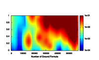
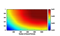
Figure 4: Row 1: Random Tractable MLNs, Row 2: FSPC MLN, Left column: ground formula, ground messages, Middle Column: lifted formula, ground messages, Right Column: lifted formula, lifted messages

The LGBP propagation algorithm only requires statistics about the number of identical messages send during message passing. Specifically, the message-update rule requires the following quantities:

1. $G_{P}(r,r_{p},R_{l})$ - the number of copies of $\langle r_{p},r\rangle\in R_{l}$ directed into a single copy of $r$ from all copies of $r_{p}$ in $R_{g}$.

2. $G_{D}(r,r_{d},R_{l})$ - the number of copies of $r_{d}$ that are descendants of a single copy of $r$ in $R_{g}$.

3. $G_{\mathcal{E}}(r,r_{d},r_{d_{p}})$ - Given lifted region nodes $r,r_{d},r_{d_{p}}$ where: (a) $r_{d}$ is a descendant of $r$ in $R_{l}$, (b) $r_{d_{p}}$ is a parent of $r_{d}$ in $R_{l}$, (c) $v_{r}\in R_{g}$ is a single copy of $r$, and (d) $v_{d_{r}}\in R_{g}$ is a single copy of $r_{d}$, $G_{\mathcal{E}}(r,r_{d},r_{d_{p}})$ is the number of copies of $r_{d_{p}}$ in $R_{g}$ (excluding $v_{r}$) that are parents of $v_{d_{r}}\in R_{g}$ but not descendants of $v_{r}\in R_{g}$.

Each of these quantities can be computed (via formulation as a CSP) without explicitly constructing the ground region graph. We omit the derivation due to space constraints.

Message Passing

We present a lifted version of the parent-to-child algorithm. Each lifted region $r$ has a belief given by $b_{r}(x_{r})=$

$$\prod_{f_{i}\in M_{r}}f_{i}\left(\prod_{r_{p}\in P(r)}m_{r_{p}\rightarrow r}^{G_{P}(r,r_{p},R_{l})}\right)\\ \left(\prod_{r_{d}\in D(r)}\left(\prod_{r^{\prime}_{p}\in P(r_{d})}m_{r^{\prime}_{p}\rightarrow r_{d}}^{G_{\mathcal{E}}(r,r_{d},r_{d_{p}},R_{l})}\right)^{G_{D}(r,r_{d},R_{l})}\right)$$ (2)

Here $P(r)$ is the set of lifted regions that are parents to lifted region $r$ and $D(r)$ is the set of all lifted regions that are descendants of lifted region $r$. The message-update rule for $m_{r_{p}\rightarrow r}$ is obtained by setting the beliefs at regions $r$ and $r_{p}$ to be equal over their message variables, and is given by $m_{r_{p}\rightarrow r}(x_{R})=$

$$\frac{\sum_{x_{P\setminus R}}b_{p}(x_{r})}{\left(\prod_{f_{i}\in M_{r}}f_{i}\right)\left(m_{r_{p}\rightarrow r}^{G_{P}(r,r_{p})-1}\right)\left(\prod_{r_{p}^{\prime}\in P^{\prime}(r,r_{p})}m_{r_{p}^{\prime}\rightarrow r}^{G_{P}(r,r_{p}^{\prime})}\right)}$$ (3)

where $P^{\prime}(r,r_{p})$ is the set of lifted regions that are parents of $r$ in $R_{l}$ excluding $r_{p}$.

Intra-Region Inference and Region Graph Construction

Each message $m_{r_{p}\rightarrow r}(x_{R})$ is computed in the parent region, $r_{p}=\langle M_{p},V_{pg},E_{r_{p}g}\rangle$ by running inference over the lifted factorization of a single grounding of $r_{p}$ given by $E_{r_{p}g}$. Inference is handled via any exact lifted inference algorithm (?; ?; ?; ?).

LGBP is a general method that works on any valid lifted region graph. A natural construction method is to heuristically grouping formulas based on the cost of lifted inference and then apply either (1) the variational cluster method (?) or (2) a mini-bucket based scheme (?) over the intersections of efficiently available sets of marginals.

Related Work

Lifting LBP relies on the observation that the factor graph structure gives rise to message-level symmetries when applied to SRMs (?). Both FOBP (?) and Counting Belief Propagation (?) propose algorithms to exploit these message-level symmetries. FOBP presents an iterative algorithm for shattering a MLN and a set of evidence into a lifted factor graph upon which messages are split into groups guaranteed to be identical on every iteration. CBP compresses a propositional factor graph by identifying identical messages and lifting over them. LGBP differs from both of these algorithms in that they perform the intra-cluster exact inference step on the propositional level, while LBGP can exploit symmetries present in each region as well as the structure of the messages being passed.

The Lifted RCR algorithm (LRCR) (?) lifts the propositional RCR algorithm (?). The RCR algorithm is a generalization of GBP in which equality constraints between random variables in different potentials are relaxed, these relaxations are compensated for (e.g. via message passing), and then some constraints are recovered, based on a heuristic. LRCR extends this framework to lifted models. Like LGBP, LRCR uses lifted inference to allow dramatically larger scopes at each region. However, LRCR still performs the ‘compensate‘ step by passing messages over the marginals of single ground variables. LGBP goes one step further; when possible it passes compact messages over the joint distribution of exchangeable variables, thus yielding a region with fewer edges.

More recently, researchers have introduced symmetry-exploiting techniques that permit formulation of the approximate inference task as an efficient optimization problem These methods admit a reparameterization SRM inference over a reduced variable space; the problem can then be solved by standard LP techniques for MAP inference (?) and by variational methods for marginal inference (?; ?).

Experimental Results

We conduct two sets of experiments. We focus on models which are amenable to exact inference so that we can compare accuracy of different message passing structures.

Random Tractable Models

We generated 1000 sets of 15 first-order clauses, $\{KB_{1},\ldots,KB_{1000}\}$. Each clause is of the form $x\vee y\vee z$, where $x,y,z$ are randomly selected from the set $\{R_{1}(x_{1}),\ldots,R_{15}(x_{15})\}$. For each $KB_{i},$ variance $\sigma\in\{0.0,0.1,\ldots,1.0\},$ and domain size $d\in\{1,\ldots,20\}$, we generate an MLN by assigning the domain of all variables in $KB_{i}$ to $\{1,\ldots,d\}$ and assigning each clause in $KB_{i}$ a weight sampled from $\mathcal{N}(0,\sigma)$.

For each randomly generated MLN, we construct three lifted region graphs. All region graphs place a single lifted formula in each top level region. The first region graph grounds the top level formula and passes messages over ground variables, similar to FOBP. The second region graph builds a lifted factorization of all ground formulas in each top level cluster, but passes messages over ground variables. The third region graph builds a lifted factorization of each cluster, and communicates via joint messages over exchangeable atoms when the structure allows. For each model, we compute the true marginals over each lifted atom, and then compute the KL-divergence of these (single variable) marginals from those returned by LGBP. Figure 4(top) shows KL-divergence as a function of variance and domain size for each structure. The results show that the lifted region graph structure returns accurate results for a significantly larger range of domain size and variance than either of the other structures.

Friends, Smokers, Parents, Cancer MLN Results

The second experimental setup mirrors the first; however all 1000 runs of the algorithm are performed on the same model, a complication of the Friends and Smokers MLN:

$$\langle Smokes(x)\wedge Friends(x,y)\rightarrow Smokes(y)\rangle$$

$$\langle Smokes(x)\rightarrow Cancer(x)\rangle$$

$$\langle Cancer(y)\wedge ParentOf(y,x)\rightarrow Cancer(x)\rangle$$

$$\langle Smokes(y)\wedge ParentOf(x,y)\rightarrow Smokes(x)\rangle$$

We also added formulas for each singleton atom. Again we randomly generated weights as per the procedure detailed for random models, and we ran the algorithm 1000 times on the same three types of region graphs. Figure 4(bottom) shows KL-divergence as a function of variance and domain size for each algorithm. Figure 4 demonstrates that while FOBP can yield quite accurate results in some cases, it is not resilient to large variance in formula weights, and that increasing the domain size can further exacerbate its accuracy. We observed that FOBP region graph structure generally takes more iterations than either of the other region graph structures, and often fails to converge for even moderately diverse weights. Clustering groundings of the same formula offers a significant improvement in both convergence and accuracy of the returned results. We observed that the addition of joint message passing requires slightly more iterations, but will converge to superior results on a wider variety of models.

Conclusions and Future Work

For message-passing based inference methods in PGMs, one strategy for realizing accurate approximations is to reduce the number of edges in the message-passing structure. By exploiting techniques for exact lifted inference, we have extended this strategy to SRMs. We have presented a Lifted Generalized Belief Propagation algorithm and demonstrated that the algorithm improves the overall accuracy of the approximation on a number of models. For future work, our first goal is to develop a lifted region graph construction algorithm that clusters formulas into top-level regions such that (1) the complexity of inference at each cluster is bounded, and (2) the number of messages in the model is minimized. Second, we aim to employ the LGBP algorithm for efficient weight learning over large and complicated models. Third, we aim to generalize inference over the lifted region graph structure to algorithms using lifted variational inference principles (?).

Acknowledgements

This research was funded by the Defense Advanced Research Projects Agency (DARPA) Probabilistic Programming for Advanced Machine Learning (PPAML) Program under Air Force Research Laboratory (AFRL) prime contract no. FA8750-14-C-0005.

References

- [Bui, Huynh, and Riedel 2013] Bui, H.; Huynh, T.; and Riedel, S. 2013. Automorphism groups of graphical models and lifted variational inference. In Proceedings of the Twenty-Nineth Conference on Uncertainty in Artificial Intelligence, 132–141.
- [Bui, Huynh, and Sontag 2014] Bui, H. H.; Huynh, T. N.; and Sontag, D. 2014. Lifted tree-reweighted variational inference. In Proceedings of the Thirtieth Conference on Uncertainty in Artificial Intelligence (UAI-14).
- [Choi and Darwiche 2010] Choi, A., and Darwiche, A. 2010. Relax, Compensate and Then Recover. volume 6797 of Lecture Notes in Computer Science, 167–180. Springer.
- [de Salvo Braz 2007] de Salvo Braz, R. 2007. Lifted First-Order Probabilistic Inference. Ph.D. Dissertation, University of Illinois, Urbana-Champaign, IL.
- [Dechter, Kask, and Mateescu 2002] Dechter, R.; Kask, K.; and Mateescu, R. 2002. Iterative join-graph propagation. In Proceedings of the Eighteenth conference on Uncertainty in artificial intelligence, 128–136.
- [Gogate and Domingos 2011] Gogate, V., and Domingos, P. 2011. Probabilistic Theorem Proving. In Proceedings of the Twenty-Seventh Conference on Uncertainty in Artificial Intelligence, 256–265.
- [Gogate, Jha, and Venugopal 2012] Gogate, V.; Jha, A.; and Venugopal, D. 2012. Advances in Lifted Importance Sampling. In Proceedings of the Twenty-Sixth AAAI Conference on Artificial Intelligence.
- [Jaimovich, Meshi, and Friedman 2012] Jaimovich, A.; Meshi, O.; and Friedman, N. 2012. Template based inference in symmetric relational markov random fields. arXiv preprint arXiv:1206.5276.
- [Kersting, Ahmadi, and Natarajan 2009] Kersting, K.; Ahmadi, B.; and Natarajan, S. 2009. Counting Belief Propagation. In Proceedings of the Twenty-Fifth Conference on Uncertainty in Artificial Intelligence, 277–284.
- [Kikuchi 1951] Kikuchi, R. 1951. A theory of cooperative phenomena. Physical review 81(6):988.
- [Mittal et al. 2015] Mittal, H.; Mahajan, A.; Gogate, V.; and Singla, P. 2015. Lifted inference rules with constraints. In Advances in Neural Information Processing Systems, 3501–3509.
- [Mladenov and Kersting 2015] Mladenov, M., and Kersting, K. 2015. Equitable partitions of concave free energies. Proc. of UAI-15.
- [Mladenov, Globerson, and Kersting 2014] Mladenov, M.; Globerson, A.; and Kersting, K. 2014. Lifted message passing as reparametrization of graphical models. In Proc. of UAI, 603–612.
- [Pearl 1988] Pearl, J. 1988. Probabilistic Reasoning in Intelligent Systems: Networks of Plausible Inference. San Francisco, CA: Morgan Kaufmann.
- [Poole 2003] Poole, D. 2003. First-Order Probabilistic Inference. In Proceedings of the 18th International Joint Conference on Artificial Intelligence, 985–991.
- [Richardson and Domingos 2006] Richardson, M., and Domingos, P. 2006. Markov logic networks. Machine learning 62(1-2):107–136.
- [Singla and Domingos 2008] Singla, P., and Domingos, P. 2008. Lifted First-Order Belief Propagation. In Proceedings of the Twenty-Third AAAI Conference on Artificial Intelligence, 1094–1099.
- [Smith and Gogate 2015] Smith, D., and Gogate, V. 2015. Bounding the cost of search-based lifted inference. In Advances in Neural Information Processing Systems, 946–954.
- [Van den Broeck et al. 2011] Van den Broeck, G.; Taghipour, N.; Meert, W.; Davis, J.; and De Raedt, L. 2011. Lifted Probabilistic Inference by First-Order Knowledge Compilation. In Proceedings of the 22nd International Joint Conference on Artificial Intelligence, 2178–2185.
- [Van den Broeck, Choi, and Darwiche 2012] Van den Broeck, G.; Choi, A.; and Darwiche, A. 2012. Lifted relax, compensate and then recover: From approximate to exact lifted probabilistic inference. In Proceedings of the Twenty-Eigth Conference on Uncertainty in Artificial Intelligence.
- [Venugopal and Gogate 2012] Venugopal, D., and Gogate, V. 2012. On lifting the gibbs sampling algorithm. In Proceedings of the Twenty-Sixth Annual Conference on Neural Information Processing Systems (NIPS), 1664–1672.
- [Weiss 2000] Weiss, Y. 2000. Correctness of local probability propagation in graphical models with loops. Neural computation 12(1):1–41.
- [Yedidia, Freeman, and Weiss 2005] Yedidia, J.; Freeman, W.; and Weiss, Y. 2005. Constructing free-energy approximations and generalized belief propagation algorithms. Information Theory, IEEE Transactions on 51(7):2282–2312.