Abstract

The task of aggregating and denoising crowd-labeled data has gained increased significance with the advent of crowdsourcing platforms and massive datasets. We propose a permutation-based model for crowd labeled data that is a significant generalization of the classical Dawid-Skene model, and introduce a new error metric by which to compare different estimators. We derive global minimax rates for the permutation-based model that are sharp up to logarithmic factors, and match the minimax lower bounds derived under the simpler Dawid-Skene model. We then design two computationally-efficient estimators: the WAN estimator for the setting where the ordering of workers in terms of their abilities is approximately known, and the OBI-WAN estimator where that is not known. For each of these estimators, we provide non-asymptotic bounds on their performance. We conduct synthetic simulations and experiments on real-world crowdsourcing data, and the experimental results corroborate our theoretical findings.

1 Introduction

Recent years have witnessed a surge of interest in the use of crowdsourcing for labeling massive datasets. Expert labels are often difficult or expensive to obtain at scale, and crowdsourcing platforms allow for the collection of labels from a large number of low-cost workers. This paradigm, while enabling several new applications of machine learning, also introduces some key challenges: first, low-cost workers are often non-experts and the labels they produce can be quite noisy, and second, data collected in this fashion has a high amount of heterogeneity with significant differences in the quality of labels across workers and tasks. Thus, it is important to develop realistic models and scalable algorithms for aggregating and drawing meaningful inferences from the noisy labels obtained via crowdsourcing.

This paper focuses on objective labeling tasks involving binary choices, meaning that each question or task is associated with a single correct binary answer or label. There is a vast literature on the problem of estimation from noisy crowdsourced labels (e.g., [39, 33, 22, 21, 15, 28, 14, 5, 48, 13]). The bulk of this past work is based on the classical Dawid-Skene model [6], in which each worker $i$ is associated with a single scalar parameter $q^{\mbox{\tiny DS}}_{i}\in[0,1]$, and it is assumed that the probability that worker $i$ answers any question $j$ correctly is given by the same scalar $q^{\mbox{\tiny DS}}_{i}$. Thus, the Dawid-Skene model imposes a homogeneity condition on the questions, one which is often not satisfied in practical applications where some questions may be more difficult than others. We note that the original model by Dawid and Skene [6] also allows for asymmetric errors across different classes. In this paper, we focus on the setting with symmetric error probabilities, that has popularly come to be known as the “one-coin Dawid-Skene model”, and has been the focus of much of past literature [22, 21, 15, 5]. Both the asymmetric and symmetric models, however, are governed by restrictive parameter-based assumptions and assume homogeneity of questions.

Accordingly, in this paper, we propose and analyze a more general permutation-based model that allows the noise in the answer to depend on the particular question-worker pair. Within the context of such models, we propose and analyze a variety of estimation algorithms. One possible metric for analysis is the Hamming error, and there is a large body of past work [22, 21, 15, 14, 5, 48, 13] that provide sufficient conditions that guarantee zero Hamming error—meaning that every question is answered correctly—with high probability. Although the Hamming error can be suitable for the analysis of Dawid-Skene style models, we argue in the sequel that it is less appropriate for the heterogenous settings studied in this paper. Instead, when tasks have heterogenous difficulties, it is more natural to use a weighted metric that also accounts for the underlying difficulty of the tasks. Concretely, an estimator should be penalized less for making an error on a question that is intrinsically more difficult. In this paper, we introduce and provide analysis under such a difficulty-weighted error metric.

From a high-level perspective, the contributions of this paper can be summarized as follows:

• We introduce a new “permutation-based” model for crowd-labeled data, which is considerably richer than the popular Dawid-Skene class of models.

• In order to incorporate the richness in the model, we introduce a new difficulty-weighted loss that extends the popular Hamming loss. We prove non-asymptotic upper and lower bounds on the global minimax error under the difficulty-weighted loss, sharp up to logarithmic factors, for estimation under the permutation-based model. These bounds match those under the Dawid-Skene model up to logarithmic factors.

• We propose a computationally-efficient estimator, termed the WAN estimator, for the setting where an approximate ordering of the workers in terms of their abilities is known. We show that under the permutation-based model, this estimator has strong guarantees for the 0-1 loss and also achieves the global minimax limits (up to logarithmic factors) for the difficulty-reweighted loss.

• We provide a computationally-efficient estimator, termed the OBI-WAN estimator, when no prior information about the workers is known. This estimator achieves strong guarantees for the 0-1 loss under the Dawid-Skene model and an intermediate model, and simultaneously also has guarantees over the much richer permutation-based model thereby establishing its robustness to model specification.

• We conduct synthetic simulations as well as real-world experiments using data from the Amazon Mechanical Turk crowdsourcing platform. These experiments reveal a strong performance of the OBI-WAN estimator in practice.

The remainder of this paper is organized as follows. In Section 2, we provide some background, setup the problems we address in this paper, and provide an overview of related literature. Section 3 is devoted to our main results. We present numerical simulations and real-world experiments in Section 4. We present proofs of the claimed theoretical results in Section 5. We conclude the paper with a discussion of future research directions in Section 6.

2 Background and model formulation

We begin with some background on existing crowd-labeling models, followed by an introduction to our proposed models; we conclude with a discussion of related work.

2.1 Observation model

Consider a crowdsourcing system that consists of $n$ workers and $d$ questions. We assume every question has two possible answers, denoted by $\{-1,+1\}$, of which exactly one is correct. We let $x^{*}\in\{-1,1\}^{d}$ denote the binary vector of correct answers to all $d$ questions. We model the question-answering via an unknown matrix ${Q}^{*}\in[0,1]^{n\times d}$ whose $(i,j)^{th}$ entry, ${Q}^{*}_{ij}$, represents the probability that worker $i$ answers question $j$ correctly. Otherwise, with probability $1-{Q}^{*}_{ij}$, worker $i$ gives the incorrect answer to question $j$. For future reference, note that the (one-coin) Dawid-Skene model involves a special case of such a matrix, namely one of the form ${Q}^{*}=q^{\mbox{\tiny DS}}1^{T}$, where the vector $q^{\mbox{\tiny DS}}\in[0,1]^{n}$ corresponds to the vector of correctness probabilities, with a single scalar associated with each worker.

We denote the response of worker $i$ to question $j$ by a variable $Y_{ij}\in\{-1,0,1\}$, where we set $Y_{ij}=0$ if worker $i$ is not asked question $j$, and set $Y_{ij}$ to the answer (either $-1$ or $1$) provided by the worker otherwise. We also assume that worker $i$ is asked question $j$ with probability $p_{\mathrm{obs}}\in[0,1]$, independently for every pair $(i,j)\in[n]\times[d]$, and that a worker is never asked the same question twice. We also make the standard assumption that given the values of $x^{*}$ and ${Q}^{*}$, the entries of $Y$ are all mutually independent. In summary, we observe a matrix $Y$ which has independent entries distributed as

$$Y_{ij}=\begin{cases}x^{*}_{j}&\qquad\mbox{with probability $p_{\mathrm{obs}}\;{Q}^{*}_{ij}$}\\ -x^{*}_{j}&\qquad\mbox{with probability $p_{\mathrm{obs}}\;(1-{Q}^{*}_{ij})$}\\ 0&\qquad\mbox{with probability $(1-p_{\mathrm{obs}})$.}\end{cases}$$

Given this random matrix $Y$, our goal is to estimate the binary vector $x^{*}\in\{-1,1\}^{d}$ of true labels.

Obtaining non-trivial guarantees for this problem requires that some structure be imposed on the probability matrix ${Q}^{*}$. The Dawid-Skene model is one form of such structure: it requires that the probability matrix ${Q}^{*}$ be rank one, with identical columns all equal to $q^{\mbox{\tiny DS}}\in\mathbb{R}^{n}$. As noted previously, this structural assumption on ${Q}^{*}$ is very strong. It assumes that each worker has a fixed probability of answering a question correctly, and is likely to be violated in settings where some questions are more difficult than others.

Accordingly, in this paper, we study a more general permutation-based model of the following form. We assume that there are two underlying orderings, both of which are unknown to us: first, a permutation $\pi^{*}:[n]\rightarrow[n]$ that orders the $n$ workers in terms of their (latent) abilities, and second, a permutation $\sigma^{*}:[d]\rightarrow[d]$ that orders the $d$ questions with respect to their (latent) difficulties. In terms of these permutations, we assume that the probability matrix ${Q}^{*}$ obeys the following conditions:

• Worker monotonicity: For every pair of workers $i$ and $i^{\prime}$ such that $\pi^{*}(i)<\pi^{*}(i^{\prime})$ and every question $j$, we have ${Q}^{*}_{ij}\geq{Q}^{*}_{i^{\prime}j}$.

• Question monotonicity: For every pair of questions $j$ and $j^{\prime}$ such that $\sigma^{*}(j)<\sigma^{*}(j^{\prime})$ and every worker $i$, we have ${Q}^{*}_{ij}\geq{Q}^{*}_{ij^{\prime}}$.

In other words, the permutation-based model assumes the existence of a permutation of the rows and columns such that each row and each column of the permuted matrix ${Q}^{*}$ has non-increasing entries. The rank of the resulting matrix is allowed to be as large as $\min\{n,d\}$. It is straightforward to verify that the Dawid-Skene model corresponds to a particular type of such probability matrices, restricted to have identical columns.

In summary, we let $\mathbb{C}_{\mbox{\scalebox{0.8}{{Perm}}}}$ denote the set of all possible values of matrix ${Q}^{*}$ under the proposed permutation-based model, that is,

$$\mathbb{C}_{\mbox{\scalebox{0.8}{{Perm}}}}:\,=\big{\{}Q\in[0,1]^{n\times d}\mid (\pi,\sigma)$$ there exist permutations such that

$$\mbox{ question \& worker monotonicity hold}\big{\}}.$$

For future reference, we also use

$$\mathbb{C}_{\mbox{\scalebox{0.8}{{DS}}}}:\,=\big{\{}Q\in\mathbb{C}_{\mbox{\scalebox{0.8}{{Perm}}}}\mid Q=q^{\mbox{\tiny DS}}1^{T}\mbox{ for some $q^{\mbox{\tiny DS}}\in[0,1]^{n}$}\big{\}},$$

to denote the subset of such matrices that are realizable under the Dawid-Skene assumption.

It should be noted that none of these models are identifiable without further constraints. For instance, changing $x^{*}$ to $-x^{*}$ and ${Q}^{*}$ to $(11^{T}-{Q}^{*})$ does not change the distribution of the observation matrix $Y$. In the context of the Dawid-Skene model, several papers [22, 21, 14, 48] have resolved this issue by requiring that $\frac{1}{n}\sum_{i=1}^{n}q^{\mbox{\tiny DS}}_{i}\geq{\frac{1}{2}}+\mu$ for some constant value $\mu>0$. Although this condition resolves the lack of identifiability, the underlying assumption—namely that every question is answerable by a subset of the workers—can be violated in practice. In particular, one frequently encounters questions that are too difficult to answer by any of the hired workers, and for which the worker’s answers are near uniformly random (e.g., see the papers [8, 38]). On the other hand, empirical observations also show that workers in crowdsourcing platforms, as opposed to being adversarial in nature, at worst provide random answers to labeling tasks [47, 8, 12, 11]. On this basis, for certain results in the paper, we will consider the regime:

$${Q}^{*}_{ij}\geq{\frac{1}{2}}\qquad\forall i\in[n],j\in[d].$$ (R1)

Note that neither the condition (R1) nor the condition $\frac{1}{n}\sum_{i=1}^{n}q^{\mbox{\tiny DS}}_{i}\geq{\frac{1}{2}}+\mu$ from past literature dominate one another.

2.2 Evaluating estimators

In this section, we introduce the criteria used to evaluate estimators in this paper. In formal terms, an estimator $\widehat{x}$ is a measurable function that maps any observation matrix $Y$ to a vector in the Boolean hypercube $\{-1,1\}^{d}$. The most popular way of assessing the performance of such an estimator is in terms of its (normalized) Hamming error

$$d_{\mbox{\tiny{H}}}({\widehat{x}},{x^{*}}):\,=\frac{1}{d}\sum_{j=1}^{d}\mathbf{1}\{\widehat{x}_{j}\neq x^{*}_{j}\},\vspace{-.1cm}$$ (1)

where $\mathbf{1}\{\widehat{x}_{j}\neq x^{*}_{j}\}$ denotes a binary indicator which takes the value $1$ if $\widehat{x}_{j}\neq x^{*}_{j}$, and $0$ otherwise. A potential deficiency of the Hamming error is that it places a uniform weight on each question. As mentioned earlier, there are applications of crowdsourcing in which some subset of the questions are very difficult, and no hired worker can answer reliably. In such settings, any estimator will have an inflated Hamming error, not due to any particular deficiencies of the estimator, but rather due to the intrinsic hardness of the assigned collection of questions. This error inflation will obscure possible differences between estimators.

Our goal in choosing an appropriate loss function is to allow for evaluation and comparison of various estimators. Thus, with the aforementioned issue in mind, we an alternative error measure that weights the Hamming error with the difficulty of each task. A more general class of error measures takes the form

$$\mathcal{L}_{{Q}^{*}}(\widehat{x},x^{*})=\frac{1}{d}\sum_{j=1}^{d}\mathbf{1}\{\widehat{x}_{j}\neq x^{*}_{j}\}\Psi({Q}^{*}_{1j},\ldots,{Q}^{*}_{nj}),$$ (2)

for some function $\Psi\!:\![0,1]^{n}\rightarrow\mathbb{R}_{+}$ which captures the difficulty of estimating the answer to a question.

The ${Q}^{*}$-loss:

In order to choose a suitable function $\Psi$, we note that past work on the Dawid-Skene model [22, 21, 15, 14, 5] has shown that the quantity

$$\frac{1}{n}\sum_{i=1}^{n}(2q^{\mbox{\tiny DS}}_{i}-1)^{2},$$ (3)

popularly known as the collective intelligence of the crowd, is central to characterizing the overall difficulty of the crowd-sourcing problem under the Dawid-Skene assumption. A natural generalization, then, is to consider the weights

$$\Psi({Q}^{*}_{1j},\ldots,{Q}^{*}_{nj}) =\frac{1}{n}\sum_{i=1}^{n}\big{(}2{Q}^{*}_{ij}-1\big{)}^{2}\qquad\mbox{for each task $j\in[d]$,}$$ (4a)

which characterizes the difficulty of task $$j {Q}^{*}$$ for a given collection of workers. This choice gives rise to the -loss function

$$\mathcal{L}_{{Q}^{*}}(\widehat{x},x^{*}) :\,=\frac{1}{d}\sum_{j=1}^{d}\Big{(}\mathbf{1}\{\widehat{x}_{j}\neq x^{*}_{j}\}\;\frac{1}{n}\sum_{i=1}^{n}(2{Q}^{*}_{ij}-1)^{2}\Big{)}$$ (4b)

$$=\frac{1}{dn}|\!|\!|({Q}^{*}-\frac{1}{2}11^{T})\;\operatorname{diag}(\widehat{x}-x^{*})|\!|\!|_{{\mbox{\tiny{F}}}}^{2},$$ (4c)

where $\operatorname{diag}(\widehat{x}-x^{*})$ denotes the matrix in $\mathbb{R}^{d\times d}$ whose diagonal entries are given by the vector $\widehat{x}-x^{*}$. Note that under the Dawid-Skene model (in which ${Q}^{*}=q^{\mbox{\tiny DS}}1^{T}$), this loss function reduces to

$$\mathcal{L}_{{Q}^{*}}(\widehat{x},x^{*})=\Big{(}\frac{1}{n}\sum_{i=1}^{n}(2q^{\mbox{\tiny DS}}_{i}-1)^{2}\Big{)}\;\underbrace{\Big{(}\frac{1}{d}\sum_{j=1}^{d}\mathbf{1}\{\widehat{x}_{j}\neq x^{*}_{j}\}\Big{)}}_{d_{\mbox{\tiny{H}}}({\widehat{x}},{x^{*}})},$$ (5)

corresponding to the normalized Hamming error rescaled by the collective intelligence.

For future reference, let us summarize some properties of the function $\mathcal{L}_{{Q}^{*}}$: (a) it is symmetric in its arguments $(x^{*},\widehat{x})$, and satisfies the triangle inequality; (b) it takes values in the interval $[0,1]$; and (c) if for every question $j\in[d]$, there exists a worker $\ell\in[n]$ such that ${Q}^{*}_{\ell j}\neq{\frac{1}{2}}$, then $\mathcal{L}_{{Q}^{*}}$ defines a metric; if not, it defines a pseudo-metric.

Regime of interest:

In this paper, we focus on understanding the minimax risk as well as the risk of various computationally efficient estimators. We work in a non-asymptotic framework where we are interested in evaluating the risk in terms of the triplet $(n,d,p_{\mathrm{obs}})$. We assume that $p_{\mathrm{obs}}\geq\frac{1}{n}$, which ensures that on average, at least one worker answers any question. We also operate in the regime $d\geq n$, which is commonplace in practical applications. Indeed, as also noted in earlier works [48], typical medium or large-scale crowdsourcing tasks employ tens to hundreds of workers, while the number of questions is on the order of hundreds to many thousands. We assume that the value of $p_{\mathrm{obs}}$ is known. This is a mild assumption since it is straightforward to estimate $p_{\mathrm{obs}}$ very accurately using its empirical expectation. We encompass the aforementioned conditions as the regime:

$$p_{\mathrm{obs}}\geq\frac{1}{n}\quad\mbox{and}\quad d\geq n.$$ (R2)

2.3 Related work

Having set up our model and notation, let us now relate it to past work in the area. For the problem of crowd labeling, the Dawid-Skene model [6] is the dominant paradigm, and has been widely studied [22, 21, 15, 28, 14, 5, 48]. Some papers have studied models that generalize the Dawid-Skene model. In a recent work, Khetan and Oh [23] analyze an extension of the Dawid-Skene model where a vector $\widetilde{q}\in\mathbb{R}^{n}$, capturing the abilities of the workers, is supplemented with a second vector ${h}^{*}\in[0,1]^{d}$, and the likelihood of worker $i$ correctly answering question $j$ is set as $\widetilde{q}_{i}(1-{h}^{*}_{j}+(1-\widetilde{q}_{i}){h}^{*}_{j})$. Although this model now has $(n+d)$ parameters instead of just $n$ as in the Dawid-Skene model, it retains parametric-type assumptions. Each worker and each question is described by a single parameter, and in this model the probability of correctness takes a specific form governed by these parameters. In contrast, in the permutation-based model each worker-question pair is described by a single parameter. Our permutation-based model forms a strict superset of this class. Zhou et al. [50, 49] propose a model based on a certain minimax entropy principle, whereas Whitehill et al. [46] propose a parameter-based model that also incorporates question difficulties. However, the algorithms proposed in these papers [50, 49, 46] have yet to be rigorously analyzed.

In this paper, we introduce a class of models that are considerably more flexible than the Dawid-Skene model, as well as a novel algorithm for estimation in such models, which we equip with some theoretical guarantees. The present paper also introduces another new algorithm for the setting in which an ordering of the workers in terms of their abilities is approximately known, for instance, based on some initial test. To be clear, the results of this paper have some limitations as compared to past work on the Dawid-Skene model, and we hope that these limitations will be removed in future work on the permutation-based model. Concretely, while the present paper addresses the setting of binary labels with symmetric error probabilities, several of these prior works also address settings with more than two classes, and where the probability of error of a worker may be asymmetric across the classes. The results presented in this paper have logarithmic factor gaps, that is, the ‘optimal’ results are optimal up to logarithmic factors, as stated throughout the paper. For the Dawid-Skene model, particularly under sparse observations, the past works [22, 21, 14, 48, 23] have results with sharper logarithmic factors. Finally, the guarantees provided in past results have error exponents that adapt to the underlying signal, whereas ours do not.

A related problem in the context of crowdsourcing is to estimate pairwise outcome probabilities from pairwise comparison data. In our past work [34, 35], we have considered this problem under an assumption of “strong stochastic transitivity (SST)”, which is a regularity condition related to the permutation-based model of this paper. Accordingly, parts of our proofs make use of metric entropy calculations from this past work. Unlike our previous work, the current paper involves an unknown set of labels, as well as a significantly different observation model: in particular, the observed data couples the unknown matrix ${Q}^{*}$ with the unknown labels. Moreover, rather than estimating the unknown probabilities ${Q}^{*}$, our primary goal in this paper is to estimate these underlying labels, for which significantly different algorithmic ideas and proof techniques are required.

Finally, the problem of aggregating labels of crowdsourcing workers is conceptually similar to that of combining classifiers in an unsupervised context, each solving multiple classification problems [32, 19]. Our work has implications for this line of research as well.

3 Main results

We now turn to the statement of our main results. We use $c$, $c_{\scalebox{0.5}{\mbox{\!U}}}$, $c_{\scalebox{0.5}{\mbox{\!L}}}$, $c_{\scalebox{0.5}{\mbox{\!0}}}$, $c_{\scalebox{0.5}{\mbox{\!H}}}$ to denote positive universal constants that are independent of all other problem parameters. Recall that the ${Q}^{*}$-loss takes values in the interval $[0,1]$.

3.1 Minimax risk for estimation under the permutation-based model

We begin by proving sharp upper and lower bounds on the minimax risk for the permutation-based model $\mathbb{C}_{\mbox{\scalebox{0.8}{{Perm}}}}$. The upper bound is obtained via an analysis of the following least squares estimator

$$(\widetilde{x}_{\mbox{\tiny{LS}}},\widetilde{Q}_{\mbox{\tiny{LS}}})\in\operatornamewithlimits{arg~{}min}\limits_{x\in\{-1,1\}^{d},\ Q\in\mathbb{C}_{\mbox{\scalebox{0.8}{{Perm}}}}}|\!|\!|p_{\mathrm{obs}}^{-1}\;Y-(2Q-11^{T})\;\operatorname{diag}(x)|\!|\!|_{{\mbox{\tiny{F}}}}^{2}.$$ (6)

In order to provide some intuition for this estimator, one can show (see the proof of Theorem 1(a) for details) that the unknowns $x^{*}$ and ${Q}^{*}$ are related to the mean of the observed matrix $Y$ via the equality $\mathbb{E}[Y]=p_{\mathrm{obs}}(2{Q}^{*}-11^{T})\;\operatorname{diag}(x^{*})$. Consequently, the estimate $(\widetilde{x}_{\mbox{\tiny{LS}}},\widetilde{Q}_{\mbox{\tiny{LS}}})$ computed via the program (6) equals the true solution $(x^{*},{Q}^{*})$ when $Y$ is replaced by its population version.

We do not know of a computationally efficient way to solve the optimization problem (6). Despite this computational issue, our statistical analysis of this estimator serves to provide a benchmark for comparing other computationally-efficient estimators, to be discussed in the sequel. The following theoretical guarantees hold in the regime (R1)$\cap$(R2):

Theorem 1.

(a) For any binary vector $x^{*}\in\{-1,1\}^{d}$ and any matrix ${Q}^{*}\in\mathbb{C}_{\mbox{\scalebox{0.8}{{Perm}}}}$, the least squares estimator $\widetilde{x}_{\mbox{\tiny{LS}}}$ has error at most

$$\mathcal{L}_{{Q}^{*}}(\widetilde{x}_{\mbox{\tiny{LS}}},x^{*})\leq c_{\scalebox{0.5}{\mbox{\!U}}}\frac{1}{np_{\mathrm{obs}}}(\log d)^{2},$$ (7a)

with probability at least $$1-e^{-c_{\scalebox{0.5}{\mbox{\!H}}}d\log(dn)} \widetilde{Q}\in\mathbb{C}_{\mbox{\scalebox{0.8}{{DS}}}} \widehat{x} \widetilde{Q}$$.
(b) There exists a matrix such that any estimator (which may even know the value of ) has error at least

$$\sup\limits_{x^{*}\in\{-1,1\}^{d}}\mathbb{E}[\mathcal{L}_{\widetilde{Q}}(\widehat{x},x^{*})]\geq c_{\scalebox{0.5}{\mbox{\!L}}}\frac{1}{np_{\mathrm{obs}}}.$$ (7b)

We provide the this theorem in Sections 5.1 and 5.2. As a consequence of this result, we see that in terms of the (global) minimax risk under the ${Q}^{*}$-loss, there is only a polylogarithmic factor difference between the Dawid-Skene and the permutation-based models, despite the permutation-based model being considerably richer.

We note that while the upper bound of Theorem 1(a) is quite involved, the lower bound of Theorem 1(b) is a straightforward result of a simple “worst case” construction. This suggests that the global minimax error be augmented with an investigation of local minimax errors under various subclasses of $\mathbb{C}_{\mbox{\scalebox{0.8}{{Perm}}}}$ and various notions and values of the signal to noise ratio, which we leave as important future work.

The least squares estimator analyzed above also yields an accurate estimate of the probability matrix ${Q}^{*}$ in the Frobenius norm, useful in settings where the calibration of workers or questions might be of interest. Again, this result holds in the regime (R1)$\cap$(R2):

Corollary 1.

(a) For any $x^{*}\in\{-1,1\}^{d}$ and any ${Q}^{*}\in\mathbb{C}_{\mbox{\scalebox{0.8}{{Perm}}}}$,, the least squares estimate $\widetilde{Q}_{\mbox{\tiny{LS}}}$ has error at most

$$\frac{1}{dn}|\!|\!|\widetilde{Q}_{\mbox{\tiny{LS}}}-{Q}^{*}|\!|\!|_{{\mbox{\tiny{F}}}}^{2}\leq c_{\scalebox{0.5}{\mbox{\!U}}}\frac{1}{np_{\mathrm{obs}}}\log^{2}d,$$ (8a)

with probability at least $$1-e^{-c_{\scalebox{0.5}{\mbox{\!H}}}d\log(dn)} x^{*}\in\{-1,1\}^{d} \widehat{Q} x^{*}$$.
(b) Conversely, for any answer vector , any estimator (which is allowed to know the value of ) has error at least

$$\sup\limits_{{Q}^{*}\in\mathbb{C}_{\mbox{\scalebox{0.8}{{Perm}}}}}\mathbb{E}[\frac{1}{dn}|\!|\!|\widehat{Q}-{Q}^{*}|\!|\!|_{{\mbox{\tiny{F}}}}^{2}]\geq c_{\scalebox{0.5}{\mbox{\!L}}}\frac{1}{np_{\mathrm{obs}}}.$$ (8b)

Please see Sections 5.3 and 5.4 for the proof of this corollary.

We do not know if there exist computationally-efficient estimators that can achieve the upper bound on the sample complexity established in Theorem 1 over the entire permutation-based model class. In the following sections, we design and analyze polynomial-time estimators that have interesting (but suboptimal) guarantees over the permutation-based model and also useful guarantees over popular subclasses of the permutation-based model.

3.2 The WAN estimator: When workers’ ordering is (approximately) known

Several organizations employ crowdsourcing workers only after a thorough testing and calibration process. Motivated by this fact, we now turn to the study of the setting in which the workers are calibrated, in the sense that it is known how they are ordered in terms of their respective abilities. More formally, recall from Section 2.1 that any matrix ${Q}^{*}\in\mathbb{C}_{\mbox{\scalebox{0.8}{{Perm}}}}$ is associated with two permutations: a permutation of the workers in terms of their abilities, and a permutation of the questions in terms of their difficulty. In this section, we assume that the permutation of the workers is (approximately) known to the estimation algorithm. Note that the estimator does not know the permutation of the questions, nor does it know the values of the entries of ${Q}^{*}$.

Given a permutation $\pi$ of the workers, our estimator consists of two steps, which we refer to as Windowing and Aggregating Naïvely, respectively, and accordingly term the procedure as the WAN estimator:

• Step $1$ (Windowing): Compute the integer

  $$k_{\mbox{\scalebox{0.5}{WAN}}}\in\operatornamewithlimits{arg~{}max}_{k\in\{p_{\mathrm{obs}}^{-1}\log^{1.5}(dn),\ldots,n\}}~{}~{}~{}\sum_{j\in[d]}\mathbf{1}\Big{\{}\big{|}\sum_{i\in[k]}Y_{\pi^{-1}(i)j}\big{|}\geq\sqrt{kp_{\mathrm{obs}}\log^{1.5}(dn)}\Big{\}},$$ (9a)

  where ties in the argmax are broken arbitrarily.

• Step 2 (Aggregating Naïvely): Set $\widehat{x}_{\mbox{\scalebox{0.5}{WAN}}}(\pi)$ as a majority vote of the best $k_{\mbox{\scalebox{0.5}{WAN}}}$ workers—that is

  $$[\widehat{x}_{\mbox{\scalebox{0.5}{WAN}}}(\pi)]_{j}\in\operatornamewithlimits{arg~{}max}_{b\in\{-1,1\}}~{}~{}~{}\sum_{i=1}^{k_{\mbox{\scalebox{0.5}{WAN}}}}\mathbf{1}\{Y_{\pi^{-1}(i)j}=b\}\qquad\mbox{for every $j\in[d]$}.$$ (9b)

The windowing step finds a value $k_{\mbox{\scalebox{0.5}{WAN}}}$ such that the answers of the best $k_{\mbox{\scalebox{0.5}{WAN}}}$ workers to most questions are significantly biased towards one of the options, thereby indicating that these workers are knowledgeable—or at least, are in agreement with each other. The second step then simply takes a majority vote of this set of the best $k_{\mbox{\scalebox{0.5}{WAN}}}$ workers. We remark that it is important to choose an appropriate value of $k_{\mbox{\scalebox{0.5}{WAN}}}$ (as done in Step 1), since an overly large value could include many random workers, thereby increasing the noise in the input to the second step; on the flip side, choosing too small a value could eliminate too much of the “signal”. Both steps can be carried out in time $\mathcal{O}(nd)$.

For the case when $\pi$ is an approximate ordering, we now establish a bound on the error of the WAN estimator. For every $j\in[d]$, let ${Q}^{*}_{j}$ denote the $j^{th}$ column of ${Q}^{*}$; for any ordering $\pi$ of the workers, $Q^{\pi}_{j}$ denote the vector obtained by permuting the entries of ${Q}^{*}_{j}$ in the order given by $\pi$, that is, with the first entry of $Q^{\pi}_{j}$ corresponding to the best worker according to $\pi$, and so on. Also recall the notation $\pi^{*}$ representing the true permutation of the workers in terms of their actual abilities. As with all of our theoretical, results, the following claim holds in the regime (R1)$\cap$(R2):

Theorem 2.

For any matrix ${Q}^{*}\in\mathbb{C}_{\mbox{\scalebox{0.8}{{Perm}}}}$ and any binary vector $x^{*}\in\{-1,1\}^{d}$, suppose that the WAN estimator is provided with the permutation $\pi$ of workers. Consider the subset of the questions given by

$$J :\,=\Big{\{}j\!\in\![d]\mid\exists k_{j}\geq\frac{\log^{1.5}(dn)}{p_{\mathrm{obs}}}\mbox{~{}~{}s.t.~{}~{}}\sum_{i=1}^{k_{j}}({Q}^{*}_{\pi^{-1}(i)j}-{\frac{1}{2}})\geq\frac{3}{4}\sqrt{\frac{k_{j}}{p_{\mathrm{obs}}}\log^{1.5}(dn)}\!\Big{\}}.$$ (10a)

Then the WAN estimator correctly estimates the labels of all questions in set $$J$$ with high probability:

$$\mathbb{P}\Big{(}[\widehat{x}_{\mbox{\scalebox{0.5}{WAN}}}(\pi)]_{j}=x^{*}_{j}~{}~{}~{}\mbox{for all $j\in J$}\Big{)} \geq 1-e^{-c_{\scalebox{0.5}{\mbox{\!H}}}\log^{1.5}(dn)}.$$ (10b)

We provide the proof of Theorem 2 in Section 5.5. At a high level, the theorem says that all questions that have some reasonable signal are estimated correctly by the WAN estimator. To gain intuition behind the notion of signal in (10a), let us consider $p_{\mathrm{obs}}=1$ and consider the majority voting algorithm (that is, taking a majority vote over all $n$ workers). A straightforward application of Hoeffding’s inequality yields that for any question $j\in[d]$, the condition $\sum_{i=1}^{n}({Q}^{*}_{ij}-\frac{1}{2})=\widetilde{\Omega}(\sqrt{n})$ is sufficient for the majority voting estimator to estimate $x^{*}_{j}$ correctly (with high probability). Furthermore, in the appendix, we also show that there exist matrices ${Q}^{*}$ where this condition is also necessary. Theorem 2 says that the WAN algorithm can estimate a question correctly if there exists some subset of “top” workers (according to $\pi$), such that this condition for majority voting applies when restricted to only the answers from these workers.

While Theorem 2 (as well as other results in the sequel) focuses on exact recovery with high probability, we note that alternatively directly bounding the expected Hamming error may yield guarantees that go beyond what is captured in this result. We leave this interesting problem for future work.

Theorem 2 has an immediate corollary, one which provides guarantees on the WAN estimator in terms of certain norms of the matrix ${Q}^{*}$ which may be more interpretable, and also provides a guarantee on the ${Q}^{*}$-loss incurred by the WAN estimator. Again, these results hold in the regime (R1)$\cap$(R2).

Corollary 2.

For any matrix $${Q}^{*}\in\mathbb{C}_{\mbox{\scalebox{0.8}{{Perm}}}} x^{*}\in\{-1,1\}^{d} \pi j\in[d]$$ and any binary vector , suppose that the WAN estimator is provided with the permutation of workers. Then for every question such that

$$\|{Q}^{*}_{j}-{\frac{1}{2}}\|_{2}^{2}\geq\frac{5\log^{2.5}(dn)}{p_{\mathrm{obs}}},\quad\mbox{and}\quad\|Q^{\pi}_{j}-Q^{\pi^{*}}_{j}\|_{2}\leq\frac{\|{Q}^{*}_{j}-{\frac{1}{2}}\|_{2}}{\sqrt{9\log(dn)}},$$ (11a)

we have

$$\mathbb{P}([\widehat{x}_{\mbox{\scalebox{0.5}{WAN}}}(\pi)]_{j}=x^{*}_{j})\geq 1-e^{-c_{\scalebox{0.5}{\mbox{\!H}}}\log^{1.5}(dn)}.$$ (11b)

Consequently, if $$\pi 1-e^{-c_{\scalebox{0.5}{\mbox{\!H}}}^{\prime}\log^{1.5}(dn)}$$ is the correct permutation of the workers, then with probability at least , we have

$$\mathcal{L}_{{Q}^{*}}(\widehat{x}_{\mbox{\scalebox{0.5}{WAN}}}(\pi),x^{*})\leq c_{\scalebox{0.5}{\mbox{\!U}}}\frac{1}{np_{\mathrm{obs}}}\log^{2.5}d.$$ (11c)

Please see Section 5.6 for the proof of Corollary 2.

The conditions (11a) required for the result of Corollary 2 are sharp up to logarithmic factors in the following sense. The required approximation guarantee $\|Q^{\pi}_{j}-Q^{\pi^{*}}_{j}\|_{2}\leq\frac{\|{Q}^{*}_{j}-{\frac{1}{2}}\|_{2}}{\sqrt{9\log(dn)}}$, if weakened to $\|Q^{\pi}_{j}-Q^{\pi^{*}}_{j}\|_{2}\leq 2\|{Q}^{*}_{j}-{\frac{1}{2}}\|_{2}$, would allow for any arbitrary permutation $\pi$. This is because every permutation $\pi$ satisfies $\|Q^{\pi}_{j}-Q^{\pi^{*}}_{j}\|_{2}\leq\|Q^{\pi}_{j}-{\frac{1}{2}}\|_{2}+\|Q^{\pi^{*}}_{j}-{\frac{1}{2}}\|_{2}=2\|{Q}^{*}_{j}-{\frac{1}{2}}\|_{2}$. Secondly, there exist constants $c_{0}>0$ and $c_{\scalebox{0.5}{\mbox{\!L}}}>0$ such that if one were guaranteed a lower bound of only $\frac{c_{0}}{p_{\mathrm{obs}}}$ on $\|{Q}^{*}_{j}-{\frac{1}{2}}\|_{2}^{2}$ instead of the stated condition of $\frac{5\log^{2.5}(dn)}{p_{\mathrm{obs}}}$, then there exists a ${Q}^{*}\in\mathbb{C}_{\mbox{\scalebox{0.8}{{DS}}}}$ satisfying this weaker condition such that any estimator $\widehat{x}$ incurs an error at least $\mathbb{P}(\widehat{x}_{j}\neq x^{*}_{j})\geq c_{\scalebox{0.5}{\mbox{\!L}}}$. Furthermore, this lower bound holds not only when the ordering of workers is exactly known, but even when the entire matrix ${Q}^{*}$ is known. The proof for this claim follows from the construction in the proof of Theorem 1(b).

At this point, we recall from Theorem 1(b) the lower bound on the estimation error in the ${Q}^{*}$-loss for any estimator. This lower bound applies to estimators that know not only the ordering of the workers, but also the entire matrix ${Q}^{*}$. This lower bound matches the upper bound (11c) of Corollary 2, and the two results in conjunction imply that the bound (11c) is sharp up to logarithmic factors.

We conclude this section with a key insight obtained from our analysis of the WAN estimator.

Remark 1 (Insight for unknown worker ordering problem).

The aforementioned results for the WAN algorithm have the following useful implication for the setting when the ordering of workers is unknown, under either of the models $\mathbb{C}_{\mbox{\scalebox{0.8}{{DS}}}}$ or $\mathbb{C}_{\mbox{\scalebox{0.8}{{Perm}}}}$. For any matrix ${Q}^{*}\in\mathbb{C}_{\mbox{\scalebox{0.8}{{Perm}}}}$, there exists a set of workers $S_{{Q}^{*}}\subseteq[n]$ such that the majority vote of the answers of the workers in $S_{{Q}^{*}}$ incurs a small risk. Consequently, it suffices to design an estimator that identifies a set of good workers and computes a majority vote of their answers. The estimator need not attempt to infer the values of the entries of ${Q}^{*}$, as is otherwise required, for instance, to compute maximum likelihood estimates.

The estimator proposed in the next section is based on the observation in Remark 1.

3.3 The OBI-WAN estimator

In this section, we return to the setting where the ordering of the workers is unknown. We begin by presenting a computationally efficient estimator.

Our proposed estimator operates in two steps. The first step performs an Ordering Based on Inner-products (OBI), that is, computes an ordering of the workers based on an inner product with the data. The second step calls upon the WAN estimator from Section 3.2 with this ordering. We thus term our proposed estimator as the OBI-WAN estimator, $\widehat{x}_{\mbox{\scalebox{0.5}{OBI-WAN}}}$. In order to make its description precise, we augment the notation of the WAN estimator $\widehat{x}_{\mbox{\scalebox{0.5}{WAN}}}(\pi)$ to let $\widehat{x}_{\mbox{\scalebox{0.5}{WAN}}}(\pi,Y)$ to denote the estimate given by $\widehat{x}_{\mbox{\scalebox{0.5}{WAN}}}(\pi)$ operating on $Y$ when given the permutation $\pi$ of workers.

An important technical issue is that re-using the observe data $Y$ to both determine an appropriate ordering of workers as well as to estimate the desired answers, results in a violation of important independence assumptions. We resolve this difficulty by partitioning the set of questions into two sets, and using the ordering estimated from one set to estimate the desired answers for the other set and vice versa. We provide a careful error analysis for this partitioning-based estimator in the sequel. In more precise terms, the OBI-WAN estimator $\widehat{x}_{\mbox{\scalebox{0.5}{OBI-WAN}}}$ is defined by the following three steps:

• Step $0$ (preliminary): Split the set of $d$ questions into two sets, $T_{0}$ and $T_{1}$, with every question assigned to one of the two sets uniformly at random. Let $Y_{0}$ and $Y_{1}$ denote the corresponding submatrices of $Y$, containing the columns of $Y$ associated to questions in $T_{0}$ and $T_{1}$ respectively.

• Step $1$ (OBI): For $\ell\in\{0,1\}$, let

  $$u_{\ell}\in\operatornamewithlimits{arg~{}max}_{\|u\|_{2}=1}\|Y_{\ell}^{T}u\|_{2}$$

  denote the top eigenvector of $Y_{\ell}Y_{\ell}^{T}$; in order to resolve the global sign ambiguity of eigenvectors, we choose the global sign so that $\sum_{i\in[n]}[u_{\ell}]_{i}^{2}\mathbf{1}\{[u_{\ell}]_{i}>0\}\geq\sum_{i\in[n]}[u_{\ell}]_{i}^{2}\mathbf{1}\{[u_{\ell}]_{i}<0\}$. Let $\pi_{\ell}$ be the permutation of the $n$ workers in order of the respective entries of $u_{\ell}$ (with ties broken arbitrarily).

• Step $2$ (WAN): Compute the quantities

  $$\widehat{x}_{\mbox{\scalebox{0.5}{OBI-WAN}}}(T_{0}):\,=\widehat{x}_{\mbox{\scalebox{0.5}{WAN}}}(Y_{0},\pi_{1}),\quad\mbox{and}\quad\widehat{x}_{\mbox{\scalebox{0.5}{OBI-WAN}}}(T_{1}):\,=\widehat{x}_{\mbox{\scalebox{0.5}{WAN}}}(Y_{1},\pi_{0}),$$

  corresponding to estimates of the answers for questions in the sets $T_{0}$ and $T_{1}$, respectively.

This completes the description of the OBI-WAN algorithm.

We note that with regard to the use of the singular vectors of the observed data in the OBI step, previous works [22, 15, 32, 48, 19] also use singular vectors to estimate properties of the underlying parameters in crowdsourcing. In these previous works, this step is motivated by the fact that the spectrum of the population matrix $\mathbb{E}[YY^{T}]$ (or its mean-centered counterpart), can be related to the parameters that underlie the model.

In the next three subsections, we provide guarantees for our OBI-WAN estimator under three model classes. Importantly, the guarantees for OBI-WAN hold simultaneously for all model classes, and the estimator does not know the true class to which the data actually belongs.

3.3.1 Guarantees for OBI-WAN under an intermediate model

In addition to the Dawid-Skene and the permutation-based models introduced earlier, we study the estimation problem in an intermediate model that lies between these two models. This intermediate model introduces a parameter ${h}^{*}_{j}\in[0,1]$ that captures the difficulty of each question $j\in[d]$, along with parameters $\widetilde{q}\in\mathbb{R}^{n}$ associated with the workers as in the Dawid-Skene model. Under this intermediate model, the probability that worker $i\in[n]$ correctly answers question $j\in[d]$ (when the worker is asked the question) is given by

$$\mathbb{P}(Y_{ij}=x^{*}_{j})=\widetilde{q}_{i}(1-{h}^{*}_{j})+{\frac{1}{2}}\;{h}^{*}_{j},~{}~{}~{}\forall~{}(i,j)~{}\mathrm{such~{}that}~{}Y_{ij}\neq 0.$$ (12)

Intuitively, the parameter ${h}^{*}_{j}$ corresponds to the difficulty of question $j$. When ${h}^{*}_{j}=1$, the worker is purely stochastic and provides random guesses, while for smaller values of ${h}^{*}_{j}$ the worker is more likely to provide a correct answer.

This modeling assumption leads to the class

$$\mathbb{C}_{\mbox{\scalebox{0.8}{Int}}}:\,=\left\{Q=\widetilde{q}(1-h)^{T}+{\frac{1}{2}}\;1h^{T}\mid\mbox{for some }\widetilde{q}\in[0,\>1]^{n},~{}h\in[0,1]^{d}\right\}.$$

Note that we have the nested relation $\mathbb{C}_{\mbox{\scalebox{0.8}{{DS}}}}\subset\mathbb{C}_{\mbox{\scalebox{0.8}{Int}}}$; the Dawid-Skene model is a special case of $\mathbb{C}_{\mbox{\scalebox{0.8}{Int}}}$ corresponding to $h=0$. In the regime (R1), we further have $\mathbb{C}_{\mbox{\scalebox{0.8}{{DS}}}}\subset\mathbb{C}_{\mbox{\scalebox{0.8}{Int}}}\subset\mathbb{C}_{\mbox{\scalebox{0.8}{{Perm}}}}$.

Up to a bijective transformation of the parameters, the model (12) is identical to a recent model proposed independently by Khetan and Oh [23], where the probability of a correct answer is assumed to be $\widetilde{q}_{i}(1-{h}^{*}_{j})+(1-\widetilde{q}_{i}){h}^{*}_{j}$. The two models however arise from different conceptual motivations: Khetan and Oh consider the probability of correctness as a convex combination of the worker’s behavior $\widetilde{q}_{i}$ and the opposite behavior $(1-\widetilde{q}_{i})$, whereas our consideration of rarity of adversarial behavior leads to the probability of correctness set as a convex combination of the worker’s behavior $\widetilde{q}_{i}$ and random responses ${\frac{1}{2}}$.

We now provide exact-recovery guarantees for the OBI-WAN estimator under this intermediate model. As with our other results, the following theorem applies to the regime (R1)$\cap$(R2):

Theorem 3.

Consider any binary vector $x^{*}\in\{-1,1\}^{d}$ and any matrix ${Q}^{*}\in\mathbb{C}_{\mbox{\scalebox{0.8}{Int}}}$ associated with vectors $(\widetilde{q},h)$ satisfying $\|\widetilde{q}-{\frac{1}{2}}\|_{2}^{2}\|1-{h}^{*}\|_{2}^{2}\geq{\frac{\widetilde{c}d\log^{2.5}(dn)}{p_{\mathrm{obs}}}}$ for a large enough constant $\widetilde{c}$. Then for every question $j\in[d]$ such that

$$(1-{h}^{*}_{j})^{2}\|\widetilde{q}-{\frac{1}{2}}\|_{2}^{2}\geq\frac{5\log^{2.5}(dn)}{p_{\mathrm{obs}}},$$ (13a)

we have

$$\mathbb{P}([\widehat{x}_{\mbox{\scalebox{0.5}{OBI-WAN}}}]_{j}=x^{*}_{j})\geq 1-e^{-c_{\scalebox{0.5}{\mbox{\!H}}}\log^{1.5}(dn)}.$$ (13b)

Please see Section 5.7 for the proof of this theorem. See also Theorem 4 in the sequel, which provides a matching lower bound (up to logarithmic factors) for the special case of ${h}^{*}=0$.

We now provide some intuition about the OBI part of the OBI-WAN estimator, and we do so in the context of Theorem 3. For simplicity in this explanation, let us ignore the sample splitting step (Step 0) of the OBI-WAN algorithm and assume the OBI step (Step 1) is applied to the entire observed data $Y$. Then under the model $\mathbb{C}_{\mbox{\scalebox{0.8}{Int}}}$, we can rewrite the observation matrix as $Y=p_{\mathrm{obs}}(2\widetilde{q}-1)(1-h)^{T}\operatorname{diag}(x^{*})+W$, where $W$ is a “noise” matrix and $p_{\mathrm{obs}}(2\widetilde{q}-1)(1-h)^{T}\operatorname{diag}(x^{*})$ is the “signal” in the observed data. In this representation, the signal is a matrix of rank one, its top left singular vector equals $2\widetilde{q}-1$ (up to a scaling), and the “magnitude of the signal” is $|\!|\!|p_{\mathrm{obs}}(2\widetilde{q}-1)(1-h)^{T}\operatorname{diag}(x^{*})|\!|\!|_{{\mbox{\tiny{op}}}}=p_{\mathrm{obs}}\|2\widetilde{q}-1\|_{2}\|1-h\|_{2}$. Furthermore, we show in the proof of Theorem 3 that the “magnitude of the noise” is bounded as $|\!|\!|W|\!|\!|_{{\mbox{\tiny{op}}}}\leq c\sqrt{dp_{\mathrm{obs}}\ \mbox{polylog}(dn)}$ with high probability. Consequently when the magnitude of signal exceeds the noise (condition stated in the beginning of Theorem 3), the top left singular vector of $Y$ approximately captures the ordering of entries in $(2\widetilde{q}-1)$ that represent the worker abilities.

The following corollary now upper bounds the ${Q}^{*}$-loss for the OBI-WAN estimator under the intermediate model in the regime (R1)$\cap$(R2):

Corollary 3.

For any ${Q}^{*}\in\mathbb{C}_{\mbox{\scalebox{0.8}{Int}}}$ and any vector $x^{*}\in\{-1,1\}^{d}$, the estimate $\widehat{x}_{\mbox{\scalebox{0.5}{OBI-WAN}}}$ has error at most

$$\mathcal{L}_{{Q}^{*}}(\widehat{x}_{\mbox{\scalebox{0.5}{OBI-WAN}}},x^{*})\leq c_{\scalebox{0.5}{\mbox{\!U}}}\frac{1}{np_{\mathrm{obs}}}\log^{2.5}d,$$ (14)

with probability at least $1-e^{-c_{\scalebox{0.5}{\mbox{\!H}}}\log^{1.5}(dn)}$.

Please see Section 5.8 for the proof of this corollary. A comparison with the lower bound of Theorem 1(b) reveals that the bound (14) is tight up to logarithmic factors.

3.3.2 Guarantees for OBI-WAN under the Dawid-Skene model

In this section, we present results relating the performance of the OBI-WAN estimator under the Dawid-Skene model. Unlike the rest of the paper, in this section the simplicity of the model allows us to generalize in another direction: handling adversarial workers, that is, not being restricted to regime (R1) and allowing $q^{\mbox{\tiny DS}}_{i}<{\frac{1}{2}}$ for some workers $i\in[n]$.

We introduce some additional notation. For the vector $q^{\mbox{\tiny DS}}\in[0,1]^{n}$, we define two associated vectors $q^{\mbox{\tiny DS$+$}},q^{\mbox{\tiny DS$-$}}\in[0,1]^{n}$ as $q^{\mbox{\tiny DS$+$}}_{i}=\max\{q^{\mbox{\tiny DS}}_{i},{\frac{1}{2}}\}$ and $q^{\mbox{\tiny DS$-$}}_{i}=\min\{q^{\mbox{\tiny DS}}_{i},{\frac{1}{2}}\}$ for every $i\in[n]$. Then we have $(q^{\mbox{\tiny DS}}-{\frac{1}{2}})=(q^{\mbox{\tiny DS$+$}}-{\frac{1}{2}})+(q^{\mbox{\tiny DS$-$}}-{\frac{1}{2}})$, with $q^{\mbox{\tiny DS$+$}}$ representing normal workers and $q^{\mbox{\tiny DS$-$}}$ representing adversarial workers who are more inclined to provide incorrect answers. The following result holds in the regime (R2):

Theorem 4.

Consider any Dawid-Skene matrix of the form ${Q}^{*}=q^{\mbox{\tiny DS}}1^{T}$ for some $q^{\mbox{\tiny DS}}\in[0,1]^{n}$. Then:

1. If $\|q^{\mbox{\tiny DS$+$}}-{\frac{1}{2}}\|_{2}\geq\|q^{\mbox{\tiny DS$-$}}-{\frac{1}{2}}\|_{2}+\sqrt{\frac{4\log^{2.5}(dn)}{p_{\mathrm{obs}}}}$ and $(q^{\mbox{\tiny DS}}-{\frac{1}{2}})^{T}1\geq 0$, then for any $x^{*}\in\{-1,1\}^{d}$, the OBI-WAN estimator satisfies

   $$\mathbb{P}(\widehat{x}_{\mbox{\scalebox{0.5}{OBI-WAN}}}\;=\;x^{*})\geq 1-e^{-c_{\scalebox{0.5}{\mbox{\!H}}}\log^{1.5}(dn)}.$$ (15a)

2. Conversely, there exists a positive universal constant $c$ such that for any $q^{\mbox{\tiny DS}}\in[\frac{1}{10},\frac{9}{10}]^{n}$ with $\|q^{\mbox{\tiny DS}}-{\frac{1}{2}}\|_{2}\leq\sqrt{\frac{c}{p_{\mathrm{obs}}}}$, any estimator $\widehat{x}$ has (normalized) Hamming error at least

   $$\sup_{x^{*}\in\{-1,1\}^{d}}\mathbb{E}\big{[}\sum_{i=1}^{d}\frac{1}{d}\mathbf{1}\{\widehat{x}_{i}\neq x^{*}_{i}\}\big{]}\geq\frac{1}{10}.$$ (15b)

The proofs of the two parts of Theorem 4 are provided in Sections 5.9 and 5.10.

A couple of remarks are in order. For the following discussion, consider the two mild conditions $\|q^{\mbox{\tiny DS$+$}}-{\frac{1}{2}}\|_{2}\geq 1.01\|q^{\mbox{\tiny DS$-$}}-{\frac{1}{2}}\|_{2}$ and $(q^{\mbox{\tiny DS}}-{\frac{1}{2}})^{T}1>0$. We claim that under these mild conditions, the OBI-WAN estimator is optimal up to logarithmic factors. To see this, first observe that the lower bound in Theorem 4(b) implies that for any non-trivial recovery guarantee to hold, it must be the case that $\|q^{\mbox{\tiny DS}}-{\frac{1}{2}}\|_{2}>\sqrt{\frac{c}{p_{\mathrm{obs}}}}$ for some positive universal constant $c$. Now suppose that $\|q^{\mbox{\tiny DS}}-{\frac{1}{2}}\|_{2}>\sqrt{\frac{c^{\prime}\log^{2.5}(dn)}{p_{\mathrm{obs}}}}$ for a large enough positive constant $c^{\prime}$; observe that this condition is only a logarithmic factor away from the necessary condition. Then under the mild aforementioned conditions, we have $\|q^{\mbox{\tiny DS$+$}}-{\frac{1}{2}}\|_{2}\geq\|q^{\mbox{\tiny DS$-$}}-{\frac{1}{2}}\|_{2}+\sqrt{\frac{4\log^{2.5}(dn)}{p_{\mathrm{obs}}}}$. Part (a) of Theorem 4 then guarantees that the OBI-WAN estimator recovers the true answers $x^{*}$ with high probability.

Secondly, an application of Theorem 4 is to the setting that has been the focus of our paper, where we have no adversarial workers. In this case, we have $q^{\mbox{\tiny DS$-$}}=0$ and $q^{\mbox{\tiny DS$+$}}=q^{\mbox{\tiny DS}}$, and the upper and lower bounds match upto a logarithmic factor. The upper bound shows that when $\|q^{\mbox{\tiny DS}}-{\frac{1}{2}}\|_{2}\geq\sqrt{\frac{4\log^{2.5}(dn)}{p_{\mathrm{obs}}}}$, the Hamming error is vanishingly small, whereas the lower bound shows that there is a universal constant $c$ such that the Hamming error is essentially as large as possible when $\|q^{\mbox{\tiny DS}}-{\frac{1}{2}}\|_{2}\leq\sqrt{\frac{c}{p_{\mathrm{obs}}}}$.

3.3.3 Guarantees for OBI-WAN under the permutation-based model

The previous two subsections provided strong guarantees for OBI-WAN for exact recovery and the ${Q}^{*}$-loss under the Dawid-Skene and intermediate models. A natural question that arises then is how robust is OBI-WAN to mismatches with respect to the Dawid-Skene and intermediate models. We analyze OBI-WAN under the considerably richer permutation-based model class in this section.

Proposition 1.

Consider any matrix ${Q}^{*}\in\mathbb{C}_{\mbox{\scalebox{0.8}{{Perm}}}}$ and any binary vector $x^{*}\in\{-1,1\}^{d}$. For every question $j\in[d]$ that such that

$$\sum_{i=1}^{n}({Q}^{*}_{ij}-{\frac{1}{2}})\geq\frac{3}{4}\sqrt{\frac{n}{p_{\mathrm{obs}}}\log^{1.5}(dn)},$$ (16a)

the OBI-WAN estimator satisfies

$$\mathbb{P}([\widehat{x}_{\mbox{\scalebox{0.5}{OBI-WAN}}}]_{j}=x^{*}_{j}) \geq 1-e^{-c_{\scalebox{0.5}{\mbox{\!H}}}\log^{1.5}(dn)}.$$ (16b)

Consequently for any ${Q}^{*}\in\mathbb{C}_{\mbox{\scalebox{0.8}{{Perm}}}}$ and any $x^{*}\in\{-1,1\}^{d}$, with probability at least $1-e^{-c_{\scalebox{0.5}{\mbox{\!H}}}\log^{1.5}(dn)}$, the estimator incurs a ${Q}^{*}$-loss of at most

$$\mathcal{L}_{{Q}^{*}}(\widehat{x}_{\mbox{\scalebox{0.5}{OBI-WAN}}},x^{*})\leq c_{\scalebox{0.5}{\mbox{\!U}}}\frac{1}{\sqrt{np_{\mathrm{obs}}}}\log d.$$ (17)

See Section 5.11 for the proof of this result.

It is well known that the majority voting estimator is highly robust to model specification (see, for instance, the discussion in [14, Section 4.2]); this robustness perhaps underlies its popularity in practice. In the appendix, we show that the majority voting estimator achieves a rate $\Omega(\frac{1}{\sqrt{np_{\mathrm{obs}}}})$ in terms of the ${Q}^{*}$-loss in the worst case over the permutation-based model. Thus the guarantee (17) for OBI-WAN matches the lower bound for majority voting. However, importantly, in addition to this guarantee over $\mathbb{C}_{\mbox{\scalebox{0.8}{{Perm}}}}$, the OBI-WAN estimator simultaneously also achieves the strong exact recovery and ${Q}^{*}$-loss guarantees of Theorem 3, Corollary 3, and Theorem 4 over the simpler models $\mathbb{C}_{\mbox{\scalebox{0.8}{Int}}}$ and $\mathbb{C}_{\mbox{\scalebox{0.8}{{DS}}}}$.

4 Experiments

In this section, we report the results of a suite of experiments, on both synthetic and real-world data, so as to evaluate the OBI-WAN estimator which was introduced in Section 3.3. We compare OBI-WAN to the Spectral-EM estimator due to Zhang et al. [48], which to the best of our knowledge, has the strongest established guarantees in the literature. For the Spectral-EM estimator, we used an implementation provided by the authors of the paper [48]. The code for the OBI-WAN estimator as well as the constituent WAN estimator is freely available on the first author’s website.

4.1 Simulations

We first conduct synthetic simulations to evaluate various aspects of the algorithms. We conduct six sets of simulations as detailed below. The results from our simulations are plotted in Figure 1. The plots in the six panels (a) through (f) of the figure are discussed below.

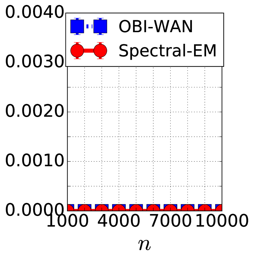
((a)) Easy

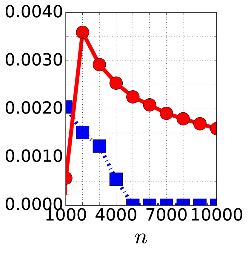
((b)) Few smart

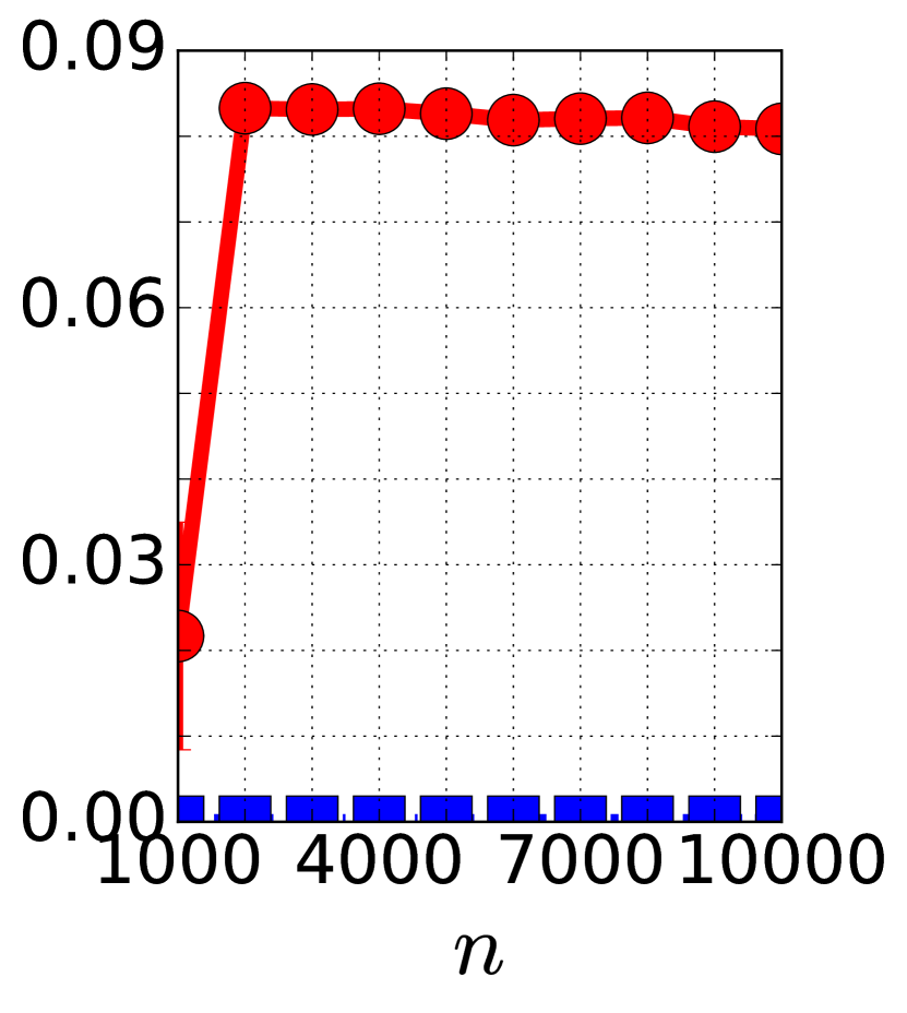
((c)) Adversarial

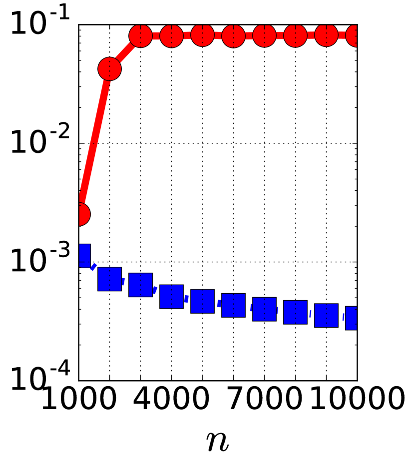
((d)) In $\mathbb{C}_{\mbox{\scalebox{0.8}{{Perm}}}}\backslash\mathbb{C}_{\mbox{\scalebox{0.8}{Int}}}$

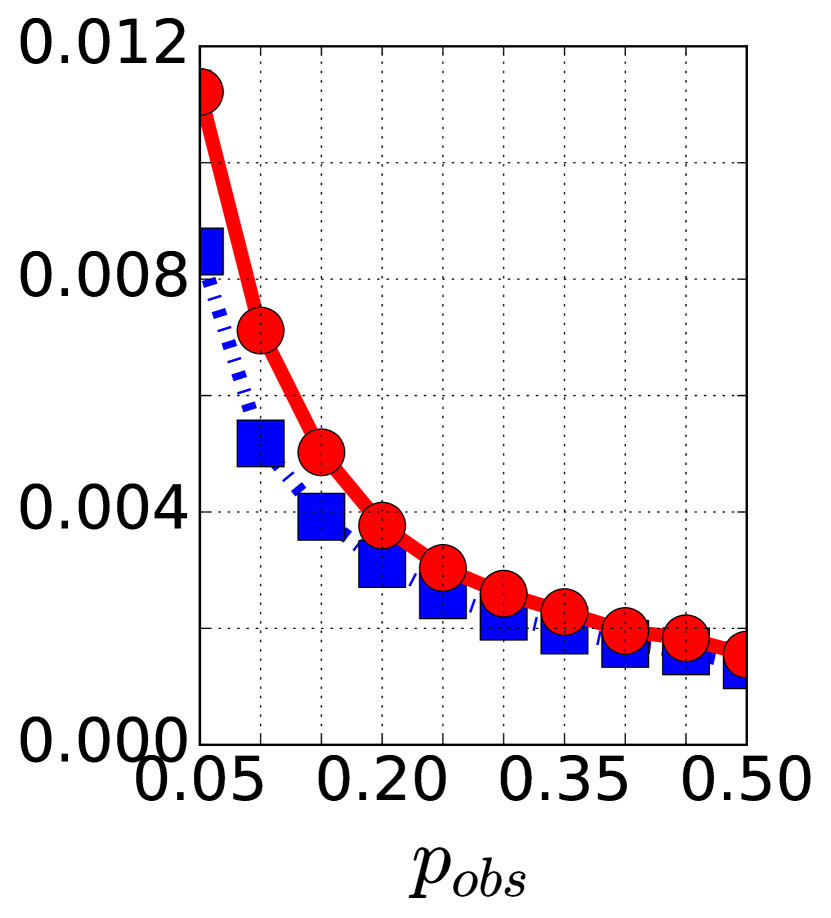
((e)) Minimax lower bound

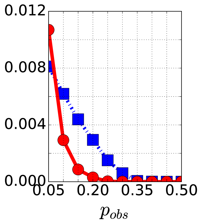
((f)) Super sparse

Figure 1: Results from numerical simulations comparing the Spectral-EM algorithm (circular markers) with OBI-WAN (square markers). The plots in panels (a)-(d) measure the ${Q}^{*}$-loss as a function of $n$, and the plots in panels (e)-(f) measure the ${Q}^{*}$-loss as a function of $p_{\mathrm{obs}}$. Each point is an average of over $20$ trials. Recall that when ${Q}^{*}$ follows the Dawid-Skene model, as in panels (a)-(c), (e)-(f), the Hamming error is proportional to the ${Q}^{*}$-loss. Also note that the Y-axis of panel (d) is plotted on a logarithmic scale.

1. Easy: ${Q}^{*}=q^{\mbox{\tiny DS}}1^{T}\in\mathbb{C}_{\mbox{\scalebox{0.8}{{DS}}}}$ where $q^{\mbox{\tiny DS}}_{i}=\frac{9}{10}$ if $i<\frac{n}{2}$, and $q^{\mbox{\tiny DS}}_{i}={\frac{1}{2}}$ otherwise. The parameter $n$ is varied, and the regime of operation is $(d=n,\;p_{\mathrm{obs}}=1)$. In this setting, both estimators correctly recover $x^{*}$.

2. Few smart: ${Q}^{*}=q^{\mbox{\tiny DS}}1^{T}\in\mathbb{C}_{\mbox{\scalebox{0.8}{{DS}}}}$ where $q^{\mbox{\tiny DS}}_{i}=\frac{9}{10}$ if $i<\sqrt{n}$, and $q^{\mbox{\tiny DS}}_{i}=\frac{1}{2}$ otherwise. The parameter $n$ is varied, and the regime of operation $(d=n,\;p_{\mathrm{obs}}=1)$. Even though the data is drawn from the Dawid-Skene model, the error of Spectral-EM is much higher than that of the OBI-WAN estimator. Recall that the OBI-WAN estimator has guarantees of recovery over the entire Dawid-Skene class, unlike the estimators in prior literature.

3. Adversarial: ${Q}^{*}=q^{\mbox{\tiny DS}}1^{T}\in\mathbb{C}_{\mbox{\scalebox{0.8}{{DS}}}}$ where $q^{\mbox{\tiny DS}}_{i}=\frac{9}{10}$ if $i<\frac{n}{4}+\sqrt{n}$, $q^{\mbox{\tiny DS}}_{i}=\frac{1}{10}$ if $i>\frac{3n}{4}$, and $q^{\mbox{\tiny DS}}_{i}=\frac{1}{2}$ otherwise. The parameter $n$ is varied, and the regime of operation is $(d=n,\;p_{\mathrm{obs}}=1)$. This set of simulations moves beyond the assumption that the entries of ${Q}^{*}$ are lower bounded by $\frac{1}{2}$, and allows for adversarial workers. The OBI-WAN estimator is successful in such a setting as well.

4. In $\mathbb{C}_{\mbox{\scalebox{0.8}{{Perm}}}}$ but outside $\mathbb{C}_{\mbox{\scalebox{0.8}{Int}}}$: ${Q}^{*}_{ij}=\frac{9}{10}$ if $(i<\sqrt{n}$ or $j<\frac{d}{2})$, and ${Q}^{*}_{ij}=\frac{1}{2}$ otherwise. The parameter $n$ is varied, and the regime of operation is $(d=n,\;p_{\mathrm{obs}}=1)$. Here we have ${Q}^{*}\in\mathbb{C}_{\mbox{\scalebox{0.8}{{Perm}}}}\backslash\mathbb{C}_{\mbox{\scalebox{0.8}{Int}}}$. The ${Q}^{*}$-loss incurred by the OBI-WAN estimator decays as $\frac{1}{\sqrt{n}}$, whereas the ${Q}^{*}$-loss of Spectral-EM remains a constant.

5. Minimax lower bound: ${Q}^{*}=q^{\mbox{\tiny DS}}1^{T}\in\mathbb{C}_{\mbox{\scalebox{0.8}{{DS}}}}$ where $q^{\mbox{\tiny DS}}_{i}=\frac{9}{10}$ if $i\leq\frac{5}{p_{\mathrm{obs}}}$ and $q^{\mbox{\tiny DS}}_{i}=\frac{1}{2}$ otherwise. The parameter $p_{\mathrm{obs}}$ is varied, and the regime of operation is $(d=1000,\;n=1000)$. This setting is the cause of the minimax lower bound of Theorem 1(b). The error of both estimators, in this case, behaves in an almost identical manner with a scaling of $\frac{1}{p_{\mathrm{obs}}}$.

6. Super sparse: ${Q}^{*}=q^{\mbox{\tiny DS}}1^{T}\in\mathbb{C}_{\mbox{\scalebox{0.8}{{DS}}}}$ where $q^{\mbox{\tiny DS}}_{i}=\frac{9}{10}$ if $i\leq\frac{n}{10}$ and $q^{\mbox{\tiny DS}}_{i}={\frac{1}{2}}$ otherwise. The parameter $p_{\mathrm{obs}}$ is varied, and the regime of operation is $(d=1000,\;n=1000)$. We see that the OBI-WAN estimator incurs a relatively higher error when data is very sparse — more generally, we have observed a higher error when $p_{\mathrm{obs}}=o(\frac{\log^{2}(dn)}{n})$, and this gap is also reflected in our upper bounds for the OBI-WAN estimator in Theorem 3(a) and Theorem 4(a) that are loose by precisely a polylogarithmic factor as compared to the associated lower bounds.

The relative benefits and disadvantages of of the proposed OBI-WAN estimator, as observed from the simulations, may be summarized as follows. In terms of limitations, the error of OBI-WAN is higher than prior works when $p_{\mathrm{obs}}$ is small (as observed in the super-sparse case) or when $n$ and $d$ are small (for instance, less than $200$). On the positive side, the simulations reveal that the OBI-WAN estimator leads to accurate estimates in a variety of settings, providing guarantees over the $\mathbb{C}_{\mbox{\scalebox{0.8}{{DS}}}}$ and $\mathbb{C}_{\mbox{\scalebox{0.8}{Int}}}$ classes, and demonstrating significant robustness in more general settings in comparison to the best known estimator in the literature.

4.2 Real-world crowdsourcing data

In this section we describe a set of six experiments conducted using real-world data from the Amazon Mechanical Turk crowdsourcing platform, ranging from visual recognition to knowledge elicitation. The experiments involved more than 200 workers in total. In each experiment, workers are asked to answer a number of questions, an we then employ statistical aggregation algorithms to estimate the ground truth answers. The results of these experiments are shown in Figure 2. As before, we compare the OBI-WAN estimator with the Spectral-EM estimator [48].

(Normalized) Hamming error

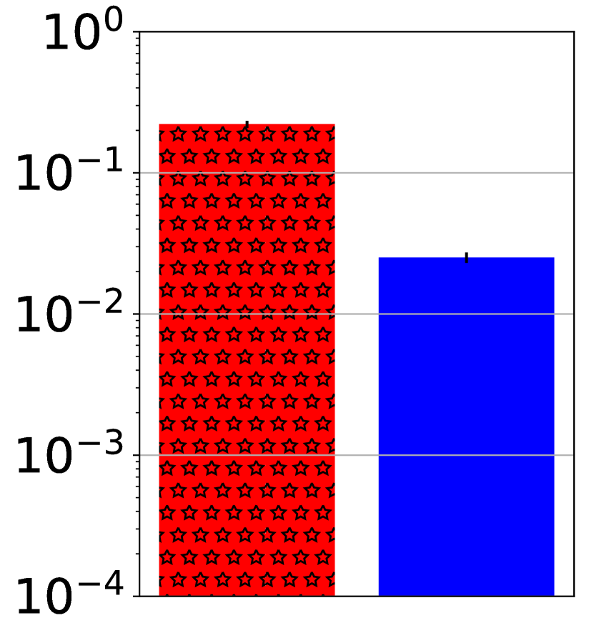
((a)) Dysplasia

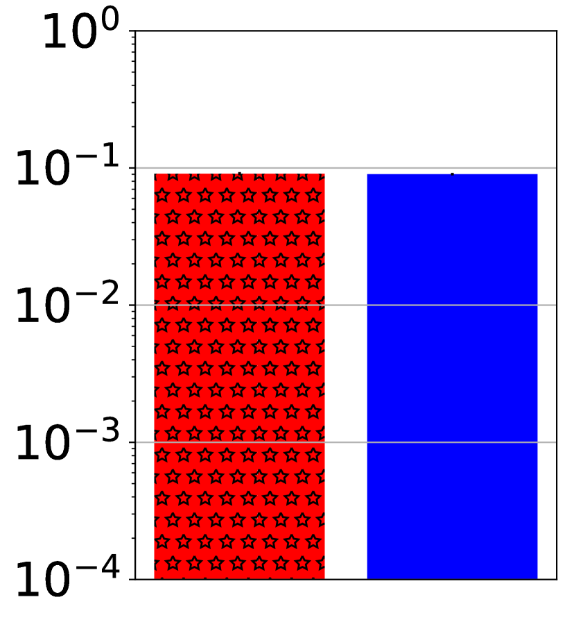
((b)) Bridges

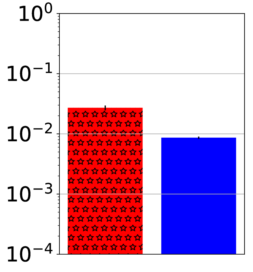
((c)) Dogs

(Normalized) Hamming error

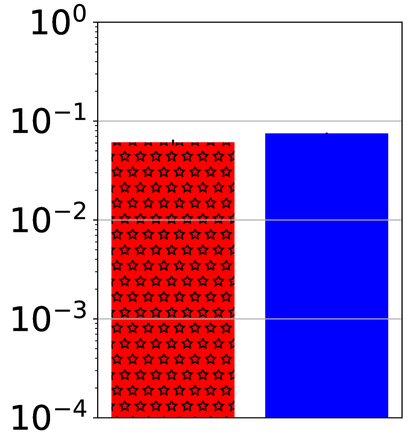
((d)) Flags

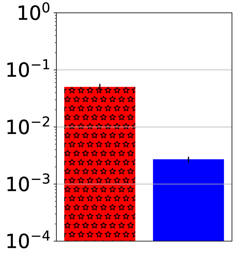
((e)) People

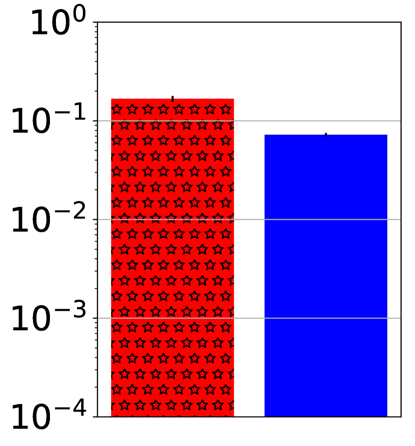
((f)) Textures

Figure 2: Results from experiments on the Amazon Mechanical Turk crowdsourcing platform comparing the Spectral-EM algorithm (left bars) with OBI-WAN (right bars). The y-axes of the plots are on a logarithmic scale and represent the Hamming error normalized by the number of questions (lower is better).

We now describe more details regarding the experiments. The error bars in each figure represent the standard error of the mean. The plots and error bars shown in each figure are obtained via 300 iterations per experiment of subsampling the worker’s answers with $p_{\mathrm{obs}}=1/3$ and executing the two algorithms on the subsampled data.

(2(a)) Dysplasia

The experiment was based on 48 pictures of (biological) cells to workers. They had to classify each image as either “Mild dysplasia” where the ratio of the nucleus’ area to cytoplasm’s area is less than 33%, or as “severe dysplasia” where the ratio of the nucleus’ area to cytoplasm’s area is more than 33%. The images and the ground truth were obtained from the DTU/Herlev Pap Smear Database 2005 [20]. We collected responses from a total of 41 workers from Amazon Mechanical Turk, and Figure 2(a) depicts the results of this experiment. The data is freely available for download on the first author’s website.

(2(b)) Bridges

The experiment was based on 21 images of bridges, and the task for any worker was to classify each image as either the golden bridge or not. The data for this experiment was collected in past work [38] from a total of 35 workers from Amazon Mechanical Turk. Figure 2(b) depicts the results from this data.

(2(c)) Dogs

The experiment comprised 85 images of dogs (from [24, 7]), and each worker was asked to identify the breed of each dog from ten provided options. The data was collected in past work [38] from a total of 35 workers from Amazon Mechanical Turk. The data is converted to binary choice form by choosing one breed uniformly at random in each iteration and considering a binary-choice task of identifying whether or not the dogs belong to this breed. Figure 2(c) plots the results of the experiments.

(2(d)) Flags

In this experiment, each worker was shown a series of 126 flags. Each question required the worker to identify if a displayed flag belonged to a place in Africa, Asia/Oceania, Europe, or neither of these. We use the data collected in the past work [38] which contains responses of 35 workers to all of the questions. We convert this data into binary choice format in the same manner as the dogs experiment above. Finally, we plot the results from this experiment in Figure 2(d).

(2(e)) People

In this experiment, the names of 20 personalities were provided and the worker were asked to classify whether they were ever the President of the USA, President of India, Prime Minister of Canada, or neither of these. Responses from 35 workers were collected in past work [38], and we convert this data to binary choice as per the aforementioned procedure. Figure 2(e) plots the results of this experiment.

(2(f)) Textures

As a final experiment, we evaluated the performance of the algorithms on workers’ classification of textures. Specifically, workers were asked to classify 24 images from the dataset [26, Dataset 1: Textured surfaces] into one of eight possible textures. We use the responses of the workers collected in [38], with a conversion to binary-choice as described above. The aggregate results from executing the two algorithms are depicted in Figure 2(f).

All in all, the experiments reveal that OBI-WAN compares favorably to Spectral-EM.

5 Proofs

In this section, we present the proofs of main theoretical results. In the proofs, we use $c$, $c_{1}$, $c^{\prime}$ etc. to denote positive universal constants, and ignore floors and ceilings unless critical to the proof. We assume that $n$ and $d$ are greater than some universal constants; the case of smaller values of these parameters are then directly implied by only changing the constant prefactors.

5.1 Proof of Theorem 1(a): Minimax upper bound

We begin by proving the minimax upper bound stated in part (a) of Theorem 1. The proof is divided into two parts, where in the first part, we obtain an upper bound on the error term $|\!|\!|(2{Q}^{*}-11^{T})\operatorname{diag}(x^{*})-(2\widetilde{Q}_{\mbox{\tiny{LS}}}-11^{T})\operatorname{diag}(\widetilde{x}_{\mbox{\tiny{LS}}})|\!|\!|_{{\mbox{\tiny{F}}}}^{2}$, following which we convert this bound to one on $\mathcal{L}_{{Q}^{*}}(x^{*},\widetilde{x}_{\mbox{\tiny{LS}}})$. follows along the lines of the proof of our previous work [34, Theorem 1(a)]. In relation of our present problem, one can think of the setting of [34] as that of estimating the matrix $(2{Q}^{*}-11^{T})$ when the value of $x^{*}$ is known. The primary additional challenge in the first part of the present proof is to accommodate the additional uncertainty about $x^{*}$.

We begin with the first part of the proof, where we bound the error in estimating the product term $(2{Q}^{*}-11^{T})\operatorname{diag}(x^{*})$. Let us rewrite our observation model in a “linearized” fashion that is convenient for subsequent analysis. In particular, let us define a random matrix $W\in\mathbb{R}^{n\times d}$ with entries independently drawn from the distribution

$$W_{ij}=\begin{cases}1-p_{\mathrm{obs}}(2{Q}^{*}_{ij}-1)x^{*}_{j}&~{}~{}~{}\mbox{w.p.~{}~{}~{}}p_{\mathrm{obs}}\Big{(}{Q}^{*}_{ij}\big{(}\frac{1+x^{*}_{j}}{2}\big{)}+(1-{Q}^{*}_{ij})\big{(}\frac{1-x^{*}_{j}}{2}\big{)}\Big{)}\\ -1-p_{\mathrm{obs}}(2{Q}^{*}_{ij}-1)x^{*}_{j}&~{}~{}~{}\mbox{w.p.~{}~{}~{}}p_{\mathrm{obs}}\Big{(}{Q}^{*}_{ij}\big{(}\frac{1-x^{*}_{j}}{2}\big{)}+(1-{Q}^{*}_{ij})\big{(}\frac{1+x^{*}_{j}}{2}\big{)}\Big{)}\\ -p_{\mathrm{obs}}(2{Q}^{*}_{ij}-1)x^{*}_{j}&~{}~{}~{}\mbox{w.p.~{}~{}~{}}1-p_{\mathrm{obs}},\end{cases}$$ (18)

where “w.p.” is a shorthand for “with probability”. One can verify that $\mathbb{E}[W]=0$, every entry of $W$ is bounded by $2$ in absolute value, and moreover that our observed matrix $Y$ can be written in the form

$$\frac{1}{p_{\mathrm{obs}}}Y=(2{Q}^{*}-11^{T})\;\operatorname{diag}(x^{*})+\frac{1}{p_{\mathrm{obs}}}W.$$ (19)

Let $\Pi_{n}$ denote the set of all permutations of the $n$ workers, and let $\Sigma_{d}$ denote the set of all permutations of the $d$ questions. For any pair of permutations $(\pi,\sigma)\in\Pi_{n}\times\Sigma_{d}$, define the set

$$\mathbb{C}_{\mbox{\scalebox{0.8}{{Perm}}}}(\pi,\sigma):\,=\Big{\{}Q\in[0,1]^{n\times d}\mid Q_{ij}\geq Q_{i^{\prime}j^{\prime}}\mbox{ whenever }$$

$$\pi(i)\leq\pi(i^{\prime})\mbox{ and }\sigma(j)\leq\sigma(j^{\prime})\Big{\}},$$

corresponding to the subset of $\mathbb{C}_{\mbox{\scalebox{0.8}{{Perm}}}}$ consisting of matrices that are faithful to the permutations $\pi$ and $\sigma$. For any fixed $x\in\{-1,1\}^{d}$, $\pi\in\Pi_{n}$ and $\sigma\in\Sigma_{d}$, define the matrix

$$\widetilde{Q}(\pi,\sigma,x) \in\operatornamewithlimits{arg~{}min}\limits_{Q\in\mathbb{C}_{\mbox{\scalebox{0.8}{{Perm}}}}(\pi,\sigma)}\mathcal{C}(Q,x),$$

$$\mbox{ where}\quad\mathcal{C}(Q,x) :\,=|\!|\!|\frac{1}{p_{\mathrm{obs}}}Y-(2Q-11^{T})\operatorname{diag}(x)|\!|\!|_{{\mbox{\tiny{F}}}}^{2}.$$

Using this notation, we can rewrite the least squares estimator (6) in the compact form

$$(\widetilde{x}_{\mbox{\tiny{LS}}},\widetilde{\pi}_{\mbox{\tiny{LS}}},\widetilde{\sigma}_{\mbox{\tiny{LS}}})\in\operatornamewithlimits{arg~{}min}\limits_{\begin{subarray}{c}(\pi,\sigma)\in\Pi_{n}\times\Sigma_{d}\\ x\in\{-1,1\}^{d}\end{subarray}}\mathcal{C}(\widetilde{Q}(\pi,\sigma,x),x),\quad\mbox{and}\quad\widetilde{Q}_{\mbox{\tiny{LS}}}=\widetilde{Q}(\widetilde{\pi}_{\mbox{\tiny{LS}}},\widetilde{\sigma}_{\mbox{\tiny{LS}}},\widetilde{x}_{\mbox{\tiny{LS}}}).$$

For the purposes of analysis, let us define the set

$${\cal P}:\,=\Big{\{}(\pi,\sigma,x)\in\Pi_{n}\times\Sigma_{d}\times\{-1,1\}^{d}\mid\mathcal{C}(\widetilde{Q}(\pi,\sigma,x),x)\leq\mathcal{C}({Q}^{*},x^{*})\Big{\}}.$$ (20)

With this set-up, we claim that it is sufficient to show the following: fix a triplet $(\pi,\sigma,x)\in{\cal P}$, for this fixed triplet there is a universal constant $c_{1}$ such that

$$\mathbb{P}\big{(}|\!|\!|(2\widetilde{Q}(\pi,\sigma,x)-11^{T})\operatorname{diag}(x-x^{*})|\!|\!|_{{\mbox{\tiny{F}}}}^{2}\leq c_{1}\frac{d}{p_{\mathrm{obs}}}\log^{2}d\big{)}\geq 1-e^{-4d\log(dn)}.$$ (21)

Given this bound, since the cardinality of the set ${\cal P}$ is upper bounded by $e^{3d\log d}$ (since $d\geq n$), a union bound over all these permutations applied to (21) yields

$$\mathbb{P}\big{(}\max_{(\pi,\sigma,x)\in{\cal P}}|\!|\!|(2\widetilde{Q}(\pi,\sigma,x)-11^{T})\operatorname{diag}(x-x^{*})|\!|\!|_{{\mbox{\tiny{F}}}}^{2}\leq c_{1}\frac{d\log^{2}d}{p_{\mathrm{obs}}}\big{)}\geq 1-e^{-d\log(dn)}.$$

The set ${\cal P}$ is guaranteed to be non-empty since the true permutations $\pi^{*}$ and $\sigma^{*}$ corresponding to ${Q}^{*}$ and the true answer $x^{*}$ always lie in ${\cal P}$, and consequently, the above tail bound yields the claimed result.

The remainder of our analysis is devoted to proving the bound (21). Given any triplet $(\pi,\sigma,x)\in{\cal P}$, we define the matrices

$$V^{*}:\,=(2{Q}^{*}-11^{T})\;\operatorname{diag}(x^{*}),~{}~{}\mbox{and}~{}~{}\widetilde{V}(\pi,\sigma,x):\,=(2\widetilde{Q}(\pi,\sigma,x)-11^{T})\;\operatorname{diag}(x).$$

Henceforth, for brevity, we refer to the matrix $\widetilde{V}(\pi,\sigma,x)$ simply as $\widetilde{V}$ and the matrix $\widetilde{Q}(\pi,\sigma,x)$ simply as $\widetilde{Q}$, since the values of the associated quantities $(\pi,\sigma,x)$ are fixed and clear from context.

Since $(\pi,\sigma,x)\in\mathcal{P}$, the definition of set $\mathcal{P}$ in (20) yields the inequality

$$|\!|\!|\frac{1}{p_{\mathrm{obs}}}Y-(2\widetilde{Q}(\pi,\sigma,x)-11^{T})\operatorname{diag}(x)|\!|\!|_{{\mbox{\tiny{F}}}}^{2}\leq|\!|\!|\frac{1}{p_{\mathrm{obs}}}Y-(2Q^{*}-11^{T})\operatorname{diag}(x^{*})|\!|\!|_{{\mbox{\tiny{F}}}}^{2}.$$

Substituting the expression $\frac{1}{p_{\mathrm{obs}}}Y=(2{Q}^{*}-11^{T})\operatorname{diag}(x^{*})+\frac{1}{p_{\mathrm{obs}}}W$ from (19), we obtain the relations

$$|\!|\!| (2{Q}^{*}-11^{T})\operatorname{diag}(x^{*})+\frac{1}{p_{\mathrm{obs}}}W-(2\widetilde{Q}(\pi,\sigma,x)-11^{T})\operatorname{diag}(x)|\!|\!|_{{\mbox{\tiny{F}}}}^{2}$$

$$\leq|\!|\!|(2{Q}^{*}-11^{T})\operatorname{diag}(x^{*})+\frac{1}{p_{\mathrm{obs}}}W-(2Q^{*}-11^{T})\operatorname{diag}(x^{*})|\!|\!|_{{\mbox{\tiny{F}}}}^{2}=|\!|\!|\frac{1}{p_{\mathrm{obs}}}W|\!|\!|_{{\mbox{\tiny{F}}}}^{2}.$$

Using the expansion $(a+b)^{2}=a^{2}+b^{2}+2ab$, and substituting the expressions for $V^{*}$ and $\widetilde{V}$, we obtain following basic inequality

$${\frac{1}{2}}|\!|\!|V^{*}-\widetilde{V}|\!|\!|_{{\mbox{\tiny{F}}}}^{2}\leq\frac{1}{p_{\mathrm{obs}}}\langle\!\langle{\widetilde{V}-V^{*}},\;{W}\rangle\!\rangle.$$ (22)

The following lemma uses this inequality to obtain an upper bound on the quantity ${\frac{1}{2}}|\!|\!|V^{*}-\widetilde{V}|\!|\!|_{{\mbox{\tiny{F}}}}^{2}$.

Lemma 1.

There exists a universal constant $c_{1}>0$ such that

$$\mathbb{P}\Big{(}|\!|\!|V^{*}-\widetilde{V}|\!|\!|_{{\mbox{\tiny{F}}}}^{2}\leq c_{1}\frac{d\log^{2}d}{p_{\mathrm{obs}}}\Big{)}\geq 1-e^{-4d\log(dn)}.$$ (23)

See Section 5.1.1 for the proof of this lemma. This completes the first part of the proof.

In the second part of the proof, we now convert our bound (23) on the Frobenius norm $|\!|\!|V^{*}-\widetilde{V}|\!|\!|_{{\mbox{\tiny{F}}}}$ into one on the error in estimating $x^{*}$ under the ${Q}^{*}$-loss. The following lemma is useful for this conversion:

Lemma 2.

For any pair of matrices $A_{1},A_{2}\in\mathbb{R}_{+}^{n\times d}$ and any pair of vectors $v_{1},v_{2}\in\{-1,1\}^{d}$, we have

$$|\!|\!|A_{1}\;\operatorname{diag}(v_{1}-v_{2})|\!|\!|_{{\mbox{\tiny{F}}}}^{2}\leq 4|\!|\!|A_{1}\;\operatorname{diag}(v_{1})-A_{2}\;\operatorname{diag}(v_{2})|\!|\!|_{{\mbox{\tiny{F}}}}^{2}.$$ (24)

See Section 5.1.2 for the proof of this claim.

Recall our assumption that every entry of the matrices ${Q}^{*}$ and $\widetilde{Q}$ is at least ${\frac{1}{2}}$. Consequently, we can apply Lemma 2 with $A_{1}=({Q}^{*}-{\frac{1}{2}}11^{T})$, $A_{2}=(\widetilde{Q}-{\frac{1}{2}}11^{T})$, $v_{1}=x^{*}$ and $v_{2}=x$ to obtain the inequality

$$|\!|\!|({Q}^{*}-{\frac{1}{2}}11^{T})\operatorname{diag}(x^{*}-x)|\!|\!|_{{\mbox{\tiny{F}}}}^{2} \leq 4|\!|\!|({Q}^{*}-{\frac{1}{2}}11^{T})\operatorname{diag}(x^{*})\!-\!(\widetilde{Q}-{\frac{1}{2}}11^{T})\operatorname{diag}(\widehat{x})|\!|\!|_{{\mbox{\tiny{F}}}}^{2}$$

$$=4|\!|\!|V^{*}-\widetilde{V}|\!|\!|_{{\mbox{\tiny{F}}}}^{2}.$$ (25)

Coupled with Lemma 1, this bound yields the desired result (21).

5.1.1 Proof of Lemma 1

Our proof of this lemma closely follows along the lines of the proof of a related result in our past work [34]. Denote the error in the estimate as $\widehat{\Delta}:\,=\widetilde{V}-V^{*}$. Then from the inequality (22), have

$$\frac{1}{2}|\!|\!|\widehat{\Delta}|\!|\!|_{{\mbox{\tiny{F}}}}^{2} \leq\frac{1}{p_{\mathrm{obs}}}\langle\!\langle{W},\;{\widehat{\Delta}}\rangle\!\rangle.$$ (26)

For the quadruplet $(\pi,\sigma,x,V^{*})$ under consideration, define the set

$$\mathbb{V}_{\mbox{\scalebox{0.5}{{DIFF}}}}(\pi,\sigma,x,V^{*}):\,=\Big{\{}\alpha(V-V^{*})\mid V=(2Q-11^{T})\operatorname{diag}(x),$$

$$Q\in\mathbb{C}_{\mbox{\scalebox{0.8}{{Perm}}}}(\pi,\sigma),\ \alpha\in[0,1]\Big{\}}.$$

Since the terms $\pi$, $\sigma$, $x$ and $V^{*}$ are fixed for the purposes of this proof, we will use the abbreviated notation $\mathbb{V}_{\mbox{\scalebox{0.5}{{DIFF}}}}$ for $\mathbb{V}_{\mbox{\scalebox{0.5}{{DIFF}}}}(\pi,\sigma,x,V^{*})$.

For each choice of radius $t>0$, define the random variable

$$Z(t) :\,=\sup_{\begin{subarray}{c}D\in\mathbb{V}_{\mbox{\scalebox{0.5}{{DIFF}}}},\\ |\!|\!|D|\!|\!|_{{\mbox{\tiny{F}}}}\leq t\end{subarray}}~{}~{}\frac{1}{p_{\mathrm{obs}}}\langle\!\langle{D},\;{W}\rangle\!\rangle.$$ (27a)

Using the basic inequality (26), the Frobenius norm error $$|\!|\!|\widehat{\Delta}|\!|\!|_{{\mbox{\tiny{F}}}}$$ then satisfies the bound

$$\frac{1}{2}|\!|\!|\widehat{\Delta}|\!|\!|_{{\mbox{\tiny{F}}}}^{2} \leq\frac{1}{p_{\mathrm{obs}}}\langle\!\langle{W},\;{\widehat{\Delta}}\rangle\!\rangle\;\leq\;Z\big{(}|\!|\!|\widehat{\Delta}|\!|\!|_{{\mbox{\tiny{F}}}}\big{)}.$$ (27b)

Thus, in order to obtain a high probability bound, we need to understand the behavior of the random quantity $$Z(t)$$.

One can verify that the set $\mathbb{V}_{\mbox{\scalebox{0.5}{{DIFF}}}}$ is star-shaped, meaning that $\alpha D\in\mathbb{V}_{\mbox{\scalebox{0.5}{{DIFF}}}}$ for every $\alpha\in[0,1]$ and every $D\in\mathbb{V}_{\mbox{\scalebox{0.5}{{DIFF}}}}$. Using this star-shaped property, we are guaranteed that there is a non-empty set of scalars $\delta_{0}>0$ satisfying the critical inequality

$$\mathbb{E}[Z(\delta_{0})] \leq\frac{\delta_{0}^{2}}{2}.$$ (27c)

Our interest is in an upper bound to the smallest (strictly) positive solution $\delta_{0}$ to the critical inequality (27c), and moreover, our goal is to show that for every $t\geq\delta_{0}$, we have $|\!|\!|\widehat{\Delta}|\!|\!|_{{\mbox{\tiny{F}}}}\leq c\sqrt{t\delta_{0}}$ with high probability.

Define a “bad” event

$$\mathcal{A}_{t} :\,=\Big{\{}\exists\Delta\in\mathbb{V}_{\mbox{\scalebox{0.5}{{DIFF}}}}\mid|\!|\!|\Delta|\!|\!|_{{\mbox{\tiny{F}}}}\geq\sqrt{t\delta_{0}}\quad\mbox{and}\quad\frac{1}{p_{\mathrm{obs}}}\langle\!\langle{\Delta},\;{W}\rangle\!\rangle\geq 2|\!|\!|\Delta|\!|\!|_{{\mbox{\tiny{F}}}}\sqrt{t\delta_{0}}\Big{\}}.$$ (28)

Now suppose the event $\mathcal{A}_{t}$ is true for some $t\geq\delta_{0}$, and let $\Delta_{0}\in\mathbb{V}_{\mbox{\scalebox{0.5}{{DIFF}}}}$ be a matrix that satisfies the two conditions required for $\mathcal{A}_{t}$ to occur. Furthermore, since $\mathbb{V}_{\mbox{\scalebox{0.5}{{DIFF}}}}$ is star-shaped, the function $Z(t)$ grows at most linearly in $t$. Consequently whenever event $\mathcal{A}_{t}$ is true, we have $|\!|\!|\Delta_{0}|\!|\!|_{{\mbox{\tiny{F}}}}\geq\delta_{0}$ and hence

$$Z(\delta_{0})\geq\frac{\delta_{0}}{|\!|\!|\Delta_{0}|\!|\!|_{{\mbox{\tiny{F}}}}}Z(|\!|\!|\Delta_{0}|\!|\!|_{{\mbox{\tiny{F}}}})\stackrel{{\scriptstyle(i)}}{{\geq}}\frac{\delta_{0}}{|\!|\!|\Delta_{0}|\!|\!|_{{\mbox{\tiny{F}}}}}\frac{1}{p_{\mathrm{obs}}}\langle\!\langle{\Delta_{0}},\;{W}\rangle\!\rangle\stackrel{{\scriptstyle(ii)}}{{\geq}}2\delta_{0}\sqrt{t\delta_{0}},$$

where inequality $(i)$ follows from the definition of function $Z$ and inequality $(ii)$ uses the second condition in the definition of event $\mathcal{A}_{t}$. As a consequence, we obtain the following bound on the probabilities of the associated events

$$\mathbb{P}[\mathcal{A}_{t}]\leq\mathbb{P}[Z(\delta_{0})\geq 2\delta_{0}\sqrt{t\delta_{0}}]\qquad\mbox{for all $t\geq\delta_{0}$.}$$

The following lemma helps control the behavior of the random variable $Z(\delta_{0})$.

Lemma 3.

For any $\delta>0$, the mean of $Z(\delta)$ is upper bounded as

$$\mathbb{E}[Z(\delta)]\leq c_{1}\frac{n+d}{p_{\mathrm{obs}}}\log^{2}(nd),$$ (29a)

and for every $$u>0$$, its tail probability is bounded as

$$\mathbb{P}\Big{(}Z(\delta)>\mathbb{E}[Z(\delta)]+u\Big{)}\leq\exp\Big{(}\frac{-c_{2}u^{2}p_{\mathrm{obs}}}{\delta^{2}+\mathbb{E}[Z(\delta)]+u}\Big{)},$$ (29b)

where $c_{1}$ and $c_{2}$ are positive universal constants.

See Section 5.1.3 for the proof of this lemma.

Setting $u=\delta_{0}\sqrt{t\delta_{0}}$ in the tail bound (29b), we find that

$$\mathbb{P}\big{(}Z(\delta_{0})>\mathbb{E}[Z(\delta_{0})]\!+\!\delta_{0}\sqrt{t\delta_{0}}\big{)}\leq\exp\!\Big{(}\frac{-c_{2}(\delta_{0}\sqrt{t\delta_{0}})^{2}p_{\mathrm{obs}}}{\delta_{0}^{2}+\mathbb{E}[Z(\delta_{0})]+\delta_{0}\sqrt{t\delta_{0}}}\Big{)},~{}\mbox{for all $t\!>\!0$.}$$

By the definition of $\delta_{0}$ in (27c), we have $\mathbb{E}[Z(\delta_{0})]\leq\delta_{0}^{2}\leq\delta_{0}\sqrt{t\delta_{0}}$ for any $t\geq\delta_{0}$, and with these relations we obtain the bound

$$\mathbb{P}[\mathcal{A}_{t}] \leq\mathbb{P}[Z(\delta_{0})\geq 2\delta_{0}\sqrt{t\delta_{0}}\big{]}\;\leq\;\exp\big{(}-\frac{c_{2}}{3}\delta_{0}\sqrt{t\delta_{0}}p_{\mathrm{obs}}\big{)},\quad\mbox{for all $t\geq\delta_{0}$.}$$

Consequently, either $|\!|\!|\widehat{\Delta}|\!|\!|_{{\mbox{\tiny{F}}}}\leq\sqrt{t\delta_{0}}$, or we have $|\!|\!|\widehat{\Delta}|\!|\!|_{{\mbox{\tiny{F}}}}>\sqrt{t\delta_{0}}$. In the latter case, conditioning on the complement $\mathcal{A}_{t}^{c}$, our basic inequality implies that $\frac{1}{2}|\!|\!|\widehat{\Delta}|\!|\!|_{{\mbox{\tiny{F}}}}^{2}\leq 2|\!|\!|\widehat{\Delta}|\!|\!|_{{\mbox{\tiny{F}}}}\sqrt{t\delta_{0}}$ and hence $|\!|\!|\widehat{\Delta}|\!|\!|_{{\mbox{\tiny{F}}}}\leq 4\sqrt{t\delta_{0}}$. Putting together the pieces yields that

$$\mathbb{P}\big{(}|\!|\!|\widehat{\Delta}|\!|\!|_{{\mbox{\tiny{F}}}}\leq 4\sqrt{t\delta_{0}}\big{)}\geq 1-\exp\big{(}-\frac{c_{2}}{3}\delta_{0}\sqrt{t\delta_{0}}p_{\mathrm{obs}}\big{)},\qquad\mbox{valid for all $t\geq\delta_{0}$.}$$ (30)

Finally, from the bound on the expected value of $Z(t)$ in Lemma 3, we see that the critical inequality (27c) is satisfied for $\delta_{0}=\sqrt{\frac{2c_{1}(n+d)}{p_{\mathrm{obs}}}}\log(nd)$. Setting $t=\delta_{0}=\sqrt{\frac{2c_{1}(n+d)}{p_{\mathrm{obs}}}}\log(nd)$ in equation (30) yields the claimed result.

5.1.2 Proof of Lemma 2

Consider any four scalars $a_{1}\geq 0,a_{2}\geq 0,b_{1}\in\{-1,1\}$ and $b_{2}\in\{-1,1\}$. If $b_{1}=b_{2}$ then

$$(a_{1}b_{1}-a_{1}b_{2})^{2}=0\leq(a_{1}b_{1}-a_{2}b_{2})^{2}.$$

Otherwise we have $b_{1}=-b_{2}$. In this case, since $a_{1}$ and $a_{2}$ have the same sign,

$$(a_{1}b_{1}-a_{2}b_{2})^{2}\geq(a_{1}b_{1})^{2}=\frac{1}{4}(a_{1}b_{1}-a_{1}b_{2})^{2}.$$

The two results above in conjunction yield the inequality $(a_{1}(b_{1}-b_{2}))^{2}\leq 4(a_{1}b_{1}-a_{2}b_{2})^{2}$. Applying the above argument to each entry of the matrices $A_{1}\operatorname{diag}(v_{1}-v_{2})$ and $(A_{1}\operatorname{diag}(v_{1})-A_{2}\operatorname{diag}(v_{2}))$ yields the claim.

5.1.3 Proof of Lemma 3

We need to prove the upper bound (29a) on the mean, as well as the tail bound (29b).

Upper bounding the mean:

We upper bound the mean by using Dudley’s entropy integral, as well as some auxiliary results on metric entropy. Given a set $\mathbb{C}$ equipped with a metric $\rho$ and a tolerance parameter $\epsilon\geq 0$, we let $\log N(\epsilon,\mathbb{C},\rho)$ denote the $\epsilon$-metric entropy of the class $\mathbb{C}$ in the metric $\rho$.

With this notation, the truncated form of Dudley’s entropy integral inequality yields

$$\mathbb{E}[Z(\delta)] \leq\frac{c}{p_{\mathrm{obs}}}\;\Big{\{}d^{-8}+\int_{\frac{1}{2}d^{-9}}^{2\sqrt{nd}}\sqrt{\log N(\epsilon,\mathbb{V}_{\mbox{\scalebox{0.5}{{DIFF}}}},|\!|\!|.|\!|\!|_{{\mbox{\tiny{F}}}})}(\Delta\epsilon)\Big{\}}.$$ (31)

The upper limit of $2\sqrt{nd}$ in the integration is due to the fact $|\!|\!|D|\!|\!|_{{\mbox{\tiny{F}}}}\leq 2\sqrt{nd}$ for every $D\in\mathbb{V}_{\mbox{\scalebox{0.5}{{DIFF}}}}$.

It is known [34] that the metric entropy of the set $\mathbb{V}_{\mbox{\scalebox{0.5}{{DIFF}}}}$ is upper bounded as

$$\log N(\epsilon,\mathbb{V}_{\mbox{\scalebox{0.5}{{DIFF}}}},|\!|\!|.|\!|\!|_{{\mbox{\tiny{F}}}}) \leq 8\frac{\max\{n,d\}^{2}}{\epsilon^{2}}\big{(}\log\frac{\max\{n,d\}}{\epsilon}\big{)}^{2}\qquad\mbox{for each $\epsilon>0$.}$$

Combining this upper bound with the Dudley entropy integral (31), and observing that the integration has $\epsilon\geq{\frac{1}{2}}d^{-9}$, the claimed upper bound (29a) follows.

Bounding the tail probability of $Z(\delta)$:

In order to establish the claimed tail bound (29b), we use a Bernstein-type bound on the supremum of empirical processes due to Klein and Rio [25, Theorem 1.1c]. In particular, this result applies to a random variable of the form $X^{\dagger}=\sup_{v\in\mathcal{V}}\langle X,\,v\rangle$, where $X=(X_{1},\ldots,X_{m})$ is a vector of independent random variables taking values in $[-1,1]$, and $\mathcal{V}$ is some subset of $[-1,1]^{m}$. Their theorem guarantees that for any $t>0$,

$$\mathbb{P}\big{(}X^{\dagger}>\mathbb{E}[X^{\dagger}]+t\big{)}\leq\exp\Biggr{(}\frac{-t^{2}}{2\sup\limits_{v\in\mathcal{V}}\mathbb{E}[\langle v,\,X\rangle^{2}]+4\mathbb{E}[X^{\dagger}]+3t}\Biggr{)}.$$ (32)

In our setting, we apply this tail bound with the choices

$$X={\frac{1}{2}}W,\quad\mbox{and}\quad X^{\dagger}={\frac{1}{2}}\sup_{\begin{subarray}{c}D\in\mathbb{V}_{\mbox{\scalebox{0.5}{{DIFF}}}},\\ |\!|\!|D|\!|\!|_{{\mbox{\tiny{F}}}}\leq\delta\end{subarray}}~{}\langle\!\langle{D},\;{W}\rangle\!\rangle={\frac{1}{2}}p_{\mathrm{obs}}Z(\delta).$$

The entries of the matrix $W$ are independently distributed with a mean of zero and a variance of at most $4p_{\mathrm{obs}}$, and are bounded in absolute value by $2$. As a result, we have $\mathbb{E}[\langle\!\langle{D},\;{W}\rangle\!\rangle^{2}]\leq 4p_{\mathrm{obs}}|\!|\!|D|\!|\!|_{{\mbox{\tiny{F}}}}^{2}\leq 4p_{\mathrm{obs}}\delta^{2}$ for every $D\in\mathbb{V}_{\mbox{\scalebox{0.5}{{DIFF}}}}$. With these assignments, inequality (32) guarantees that

$$\mathbb{P}\big{(}p_{\mathrm{obs}}Z(\delta)>p_{\mathrm{obs}}\mathbb{E}[Z(\delta)]+p_{\mathrm{obs}}u\big{)}\leq\exp\Big{(} \frac{-(up_{\mathrm{obs}})^{2}}{2p_{\mathrm{obs}}\delta^{2}+2p_{\mathrm{obs}}\mathbb{E}[Z(\delta)]+3up_{\mathrm{obs}}}\Big{)},$$

for all $u>0$, and some algebraic simplifications yield the claimed result.

5.2 Proof of Theorem 1(b): Minimax lower bound

We now turn to the proof of the minimax lower bound. For a numerical constant $\delta\in(0,\frac{1}{4})$ whose precise value is determined later, define the vector $q^{\mbox{\tiny DS}}\in[0,1]^{n}$ with entries

$$q^{\mbox{\tiny DS}}_{i}=\begin{cases}{\frac{1}{2}}+\delta&\qquad\mbox{if $i\leq\frac{1}{p_{\mathrm{obs}}}$}\\ {\frac{1}{2}}&\qquad\mbox{otherwise}.\end{cases}$$ (33)

Set the probability matrix ${Q}^{*}\in[0,1]^{n\times d}$ as ${Q}^{*}=q^{\mbox{\tiny DS}}1^{T}$. Observe that we then have ${Q}^{*}\in\mathbb{C}_{\mbox{\scalebox{0.8}{{DS}}}}$. One may assume that the matrix ${Q}^{*}$ is known to the estimator under consideration.

The Gilbert-Varshamov bound [16, 43] guarantees that for a universal constant $c>0$, there is a collection $\beta=\exp(cd)$ binary vectors—that is, a collection of vectors $\{x^{1},\ldots,x^{\beta}\}$ all belonging to the Boolean hypercube $\{-1,1\}^{d}$—such that the normalized Hamming distance (1) between any pair of vectors in this set is lower bounded as

$$d_{\mbox{\tiny{H}}}(x^{\ell},x^{\ell^{\prime}})\geq\frac{1}{10},\qquad\mbox{for every $\ell,\ell^{\prime}\in[\beta]$.}$$

For each $\ell\in[\beta]$, let $\mathbb{P}^{\ell}$ denote the probability distribution of $Y$ induced by setting $x^{*}=x^{\ell}$. For the choice of ${Q}^{*}$ specified in (33), following some algebra, we obtain a upper bound on the Kullback-Leibler divergence between any pair of distributions from this collection as

$$D_{\mathrm{KL}}(\mathbb{P}^{\ell}\|\mathbb{P}^{\ell^{\prime}})\leq c^{\prime}d\delta^{2}\qquad\mbox{for every $\ell\neq\ell^{\prime}\in[\beta]$},$$

for another constant $c^{\prime}>0$. Combining the above observations with Fano’s inequality [3] yields that any estimator $\widehat{x}$ has expected normalized Hamming error lower bounded as

$$\mathbb{E}[d_{\mbox{\tiny{H}}}(\widehat{x},x^{*})]\geq\frac{1}{20}\Big{(}1-\frac{c^{\prime}d\delta^{2}+\log 2}{\log\beta}\Big{)}.$$

Consequently, for the choice of ${Q}^{*}$ given by (33), the ${Q}^{*}$-loss is lower bounded as

$$\mathbb{E}[\mathcal{L}_{{Q}^{*}}(\widehat{x},x^{*})]=\frac{4\delta^{2}}{p_{\mathrm{obs}}}\frac{\mathbb{E}[d_{\mbox{\tiny{H}}}(\widehat{x},x^{*})]}{n}\geq\frac{4\delta^{2}}{20np_{\mathrm{obs}}}\Big{(}1-\frac{c^{\prime}d\delta^{2}+\log 2}{cd}\Big{)}\stackrel{{\scriptstyle(i)}}{{\geq}}\frac{c^{\prime\prime}}{np_{\mathrm{obs}}},$$

for some constant $c^{\prime\prime}>0$ as claimed. Here inequality (i) follows by setting $\delta$ to be a sufficiently small positive constant (depending on the values of $c^{\prime}$ and $c^{\prime\prime}$).

5.3 Proof of Corollary 1(a)

In the proof of Theorem 1(a), we showed that there is a constant $c_{1}>0$ such that

$$|\!|\!|(2{Q}^{*}-11^{T})x^{*}-(2\widetilde{Q}_{\mbox{\tiny{LS}}}-11^{T})\widetilde{x}_{\mbox{\tiny{LS}}}|\!|\!|_{{\mbox{\tiny{F}}}}^{2}\leq c_{1}\frac{d}{p_{\mathrm{obs}}}\log^{2}d,$$

with probability at least $1-e^{-d\log(dn)}$. Since all entries of the matrices $2{Q}^{*}-11^{T}$ and $2\widetilde{Q}_{\mbox{\tiny{LS}}}-11^{T}$ are non-negative, and since every entry of the vectors $x^{*}$ and $\widetilde{x}_{\mbox{\tiny{LS}}}$ lies in $\{-1,1\}$, some algebra yields the bound

$$\big{(}(2{Q}^{*}_{ij}-1)-(2[\widetilde{Q}_{\mbox{\tiny{LS}}}]_{ij}-1)\big{)}^{2}\leq\big{(}(2{Q}^{*}_{ij}-1)x^{*}_{j}-(2[\widetilde{Q}_{\mbox{\tiny{LS}}}]_{ij}-1)[\widetilde{x}_{\mbox{\tiny{LS}}}]_{j}\big{)}^{2},$$

for every $i\in[n],\;j\in[d]$. Combining these inequalities yields the claimed bound.

5.4 Proof of Corollary 1(b)

We begin by constructing a set, of cardinality $\beta$, of possible matrices ${Q}^{*}$, for some integer $\beta>1$, and subsequently we show that it is hard to identify the true matrix if drawn from this set. We begin by defining a $\beta$-sized collection of vectors $\{h^{1},\ldots,h^{\beta}\}$, all contained in the set $[{\frac{1}{2}},1]^{d}$, as follows. The Gilbert-Varshamov bound [16, 43] guarantees a constant $c\in(0,1)$ such that there exists set of $\beta=\exp(cd)$ vectors, $v^{1},\ldots,v^{\beta}\in\{-1,1\}^{d}$ with the property that the normalized Hamming distance (1) between any pair of these vectors is lower bounded as

$$d_{\mbox{\tiny{H}}}(v^{\ell},v^{\ell^{\prime}})\geq\frac{1}{10},\qquad\mbox{for every $\ell,\ell^{\prime}\in[\beta]$}.$$

Fixing some $\delta\in(0,\frac{1}{4})$, let us define, for each $\ell\in[\beta]$, the vector $h^{\ell}\in\mathbb{R}^{d}$ with entries

$$[h^{\ell}]_{j} :\,=\begin{cases}{\frac{1}{2}}+\delta&\quad\mbox{if }[v^{\ell}]_{j}=1\\ {\frac{1}{2}}&\quad\mbox{otherwise}.\end{cases}$$

For each $\ell\in[\beta]$, define the matrix $Q^{\ell}=1(h^{\ell})^{T}$, and let $\mathbb{P}^{\ell}$ denote the probability distribution of the observed data $Y$ induced by setting ${Q}^{*}=Q^{\ell}$ and $x^{*}=1$. Since the entries of $Y$ are all independent, some algebra leads to the following upper bound on the Kullback-Leibler divergence between any pair of distributions from this collection:

$$D_{\mathrm{KL}}(\mathbb{P}^{\ell}\|\mathbb{P}^{\ell^{\prime}})\leq 4p_{\mathrm{obs}}nd\delta^{2}\qquad\mbox{for every $\ell\neq\ell^{\prime}\in[\beta]$}.$$

Moreover, some simple calculation shows that the squared Frobenius norm distance between any two matrices in this collection is lower bounded as

$$|\!|\!|Q^{\ell}-Q^{\ell^{\prime}}|\!|\!|_{{\mbox{\tiny{F}}}}^{2}\geq\frac{1}{10}dn\delta^{2}\qquad\mbox{for every $\ell\neq\ell^{\prime}\in[\beta]$}.$$

Combining the above observations with Fano’s inequality [3] yields that any estimator $\widehat{Q}$ for ${Q}^{*}$ has mean squared error lower bounded as

$$\mathbb{E}[|\!|\!|{Q}^{*}-\widehat{Q}|\!|\!|_{{\mbox{\tiny{F}}}}^{2}]\geq\frac{1}{20}dn\delta^{2}\Big{(}1-\frac{4p_{\mathrm{obs}}dn\delta^{2}+\log 2}{\log\beta}\Big{)}\geq c^{\prime}\frac{d}{p_{\mathrm{obs}}},$$

where we have set $\delta^{2}=\frac{c^{\prime\prime}}{p_{\mathrm{obs}}n}$ for a small enough positive constant $c^{\prime\prime}$, where $c^{\prime}$ is another positive constant whose value may depend only on $c$ and $c^{\prime\prime}$.

5.5 Proof of Theorem 2: WAN under the permutation-based model

Observe that the windowing step of the WAN estimator identifies a group of $k_{\mbox{\scalebox{0.5}{WAN}}}$ workers such that their aggregate responses towards questions are biased (towards either answer $\{-1,1\}$) by at least $\sqrt{k_{\mbox{\scalebox{0.5}{WAN}}}p_{\mathrm{obs}}\log^{1.5}(dn)}$. We first derive three properties associated with having such a bias. These properties involve function $\gamma_{\pi}:[n]\times[d]\times\{-1,1\}\rightarrow\mathbb{R}$, where $\gamma_{\pi}(k,j,x)$ represents the amount of bias in the responses of the top $k\in[n]$ workers for question $j\in[d]$ towards the answer $x\in\{-1,1\}$:

$$\gamma_{\pi}(k,j,x):\,=\sum_{i=1}^{k}(\mathbf{1}\{Y_{\pi^{-1}(i)j}=x\}-\mathbf{1}\{Y_{\pi^{-1}(i)j}=-x\})=x\sum_{i=1}^{k}Y_{\pi^{-1}(i)j}.$$

A straightforward application of the Bernstein inequality [2], using the fact that the entries of the observed matrix $Y$ are all independent, with moments bounded as

$$\mathbb{E}[Y_{ij}]=2p_{\mathrm{obs}}({Q}^{*}_{ij}-{\frac{1}{2}})x^{*}_{j},\quad\mbox{and}\quad\mathbb{E}[Y_{ij}^{2}]=p_{\mathrm{obs}},$$

ensures that all three properties stated below are satisfied with probability at least $1-e^{c\log^{1.5}(dn)}$ for every question $j\in[d]$ and every $k\in\{p_{\mathrm{obs}}^{-1}\log^{1.5}(dn),\ldots,n\}$. For the remainder of the proof we work conditioned on the event where the following properties hold:

1. Sufficient condition for bias towards correct answer: If $\sum_{i=1}^{k}({Q}^{*}_{\pi^{-1}(i)j}-{\frac{1}{2}})\geq\frac{3}{4}\sqrt{\frac{k\log^{1.5}(dn)}{p_{\mathrm{obs}}}}$, then $\gamma_{\pi}(k,j,x^{*}_{j})\geq\sqrt{kp_{\mathrm{obs}}\log^{1.5}(dn)}$.

2. Necessary condition for bias towards any answer $x\in\{-1,1\}$: $\gamma_{\pi}(k,j,x)\geq\sqrt{kp_{\mathrm{obs}}\log^{1.5}(dn)}$ only if $x=x^{*}_{j}$ and $\sum_{i=1}^{k}({Q}^{*}_{\pi^{-1}(i)j}-{\frac{1}{2}})\geq\frac{1}{4}\sqrt{\frac{k\log^{1.5}(dn)}{p_{\mathrm{obs}}}}$.

3. Sufficient condition for aggregate to be correct: If $\sum_{i=1}^{k}({Q}^{*}_{\pi^{-1}(i)j}-{\frac{1}{2}})\geq\frac{1}{4}\sqrt{\frac{k\log^{1.5}(dn)}{p_{\mathrm{obs}}}}$, then $\gamma_{\pi}(k,j,x^{*}_{j})>0$.

We now show that when these three properties hold, for any question $j_{0}\in J$, we must have that $[\widehat{x}_{\mbox{\scalebox{0.5}{WAN}}}(\pi)]_{j_{0}}=x^{*}_{j_{0}}$. In particular, we do so by exihibiting a question that is at least as hard as $j_{0}$ on which the WAN estimator is definitely correct, and use the above properties to conclude that it therefore must also be correct on the question $j_{0}$.

Recall that by the definition (10a) of $J$, for any question $j_{0}\in J$, it must be the case that there exists a $k_{j_{0}}\geq p_{\mathrm{obs}}^{-1}\log^{1.5}(dn)$ such that

$$\sum_{i=1}^{k_{j_{0}}}({Q}^{*}_{\pi^{-1}(i)j}-{\frac{1}{2}})\geq\frac{3}{4}\sqrt{\frac{k_{j_{0}}}{p_{\mathrm{obs}}}\log^{1.5}(dn)}.$$ (34)

We define an associated set $J_{0}$ as the set of questions that are at least as easy as question $j_{0}$ according to the underlying permutation $\sigma^{*}$, that is,

$$J_{0}:\,=\{j\in[d]\mid\sigma^{*}(j)\leq\sigma^{*}(j_{0})\}.$$

By the monotonicity of the columns of ${Q}^{*}$, every question in $J_{0}$ also satisfies condition (34). For each positive integer $k$, define the set

$$J(k) :\,=\Big{\{}j\in[d]\Big{|}\gamma_{\pi}(k,j,x)\geq\sqrt{kp_{\mathrm{obs}}\log^{1.5}(dn)}\mbox{~{}~{}~{}for some~{}~{}}x\in\{-1,1\}\Big{\}}.$$

Property (P1) ensures that every question in the set $J_{0}$ is also in the set $J(k_{j_{0}})$. We then have

$$|J(k_{\mbox{\scalebox{0.5}{WAN}}})|\stackrel{{\scriptstyle(i)}}{{\geq}}|J(k_{j_{0}})|\geq|J_{0}|,$$

where step (i) uses the optimality of $k_{\mbox{\scalebox{0.5}{WAN}}}$ for the optimization problem in equation (9a). Given this, there are two possibilities: either (1) we have the equality $J(k_{\mbox{\scalebox{0.5}{WAN}}})=J_{0}$, or (2) the set $J(k_{\mbox{\scalebox{0.5}{WAN}}})$ contains some question not in the set $J_{0}$. We address each of these possibilities in turn.

Case 1: It suffices to observe by Properties (P1)–(P3), that the aggregate of the top $k_{\mbox{\scalebox{0.5}{WAN}}}$ workers is correct on every question in the set $J(k_{\mbox{\scalebox{0.5}{WAN}}})$ and this implies that it must be the case that $[\widehat{x}_{\mbox{\scalebox{0.5}{WAN}}}(\pi)]_{j_{0}}=x^{*}_{j_{0}}$ as desired.

Case 2: In this case, there is some question $j^{\prime}\notin J_{0}$ such that $\gamma_{\pi}(k_{\mbox{\scalebox{0.5}{WAN}}},j,x)\geq\sqrt{k_{\mbox{\scalebox{0.5}{WAN}}}p_{\mathrm{obs}}\log^{1.5}(dn)}$ for some $x\in\{-1,1\}$. Property (P2) guarantees that $\sum_{i=1}^{k_{\mbox{\scalebox{0.5}{WAN}}}}({Q}^{*}_{\pi^{-1}(i)j^{\prime}}-{\frac{1}{2}})\geq\frac{1}{4}\sqrt{\frac{k_{\mbox{\scalebox{0.5}{WAN}}}\log^{1.5}(dn)}{p_{\mathrm{obs}}}}$ and that $x=x^{*}_{j}$. Now, since every question easier than $j_{0}$ is in the set $J_{0}$, question $j^{\prime}$ must be more difficult than $j_{0}$, which implies that

$$\sum_{i=1}^{k_{\mbox{\scalebox{0.5}{WAN}}}}({Q}^{*}_{\pi^{-1}(i)j_{0}}-{\frac{1}{2}})\geq\frac{1}{4}\sqrt{\frac{k_{\mbox{\scalebox{0.5}{WAN}}}\log^{1.5}(dn)}{p_{\mathrm{obs}}}}.$$

Applying Property (P3), we can then conclude that $[\widehat{x}_{\mbox{\scalebox{0.5}{WAN}}}(\pi)]_{j_{0}}=x^{*}_{j_{0}}$ as desired.

5.6 Proof of Corollary 2

Theorem 2 guarantees that the WAN estimator correctly answers all questions that have some reasonable signal. Note that the set (10a) is defined in terms of the $\ell_{1}$-norm of subvectors of columns of ${Q}^{*}-{\frac{1}{2}}$, whereas the conditions

$$\|{Q}^{*}_{j}-{\frac{1}{2}}\|_{2}^{2}\geq\frac{5\log^{2.5}(dn)}{p_{\mathrm{obs}}}\quad\mbox{and}\quad\|Q^{\pi}_{j}-Q^{\pi^{*}}_{j}\|_{2}\leq\frac{\|{Q}^{*}_{j}-{\frac{1}{2}}\|_{2}}{\sqrt{9\log(dn)}}$$ (35)

in the theorem claim are in terms of the $\ell_{2}$-norm of the columns of ${Q}^{*}$. The following lemma allows us to connect the $\ell_{1}$ and $\ell_{2}$-norm constraints for any vector in a general class.

Lemma 4.

For any vector $v\in[0,1]^{n}$ such that $v_{1}\geq\ldots\geq v_{n}$, there must be some $\alpha\geq\lceil{\frac{1}{2}}\|v\|_{2}^{2}\rceil$ such that

$$\sum_{i=1}^{\alpha}v_{i}\geq\sqrt{\frac{\alpha\|v\|_{2}^{2}}{2\log n}}.$$ (36)

See Section 5.6.1 for the proof of this lemma.

We now complete the proof of the theorem. We may assume without loss of generality that the rows of ${Q}^{*}$ are ordered to be non-decreasing downwards along any column, that is, that $\pi^{*}$ is the identity permutation. Consider any question $j\in[d]$ for which the permutation $\pi$ satisfies the bounds (35). For any $\ell\in[n]$, let $g_{\ell}\in\mathbb{R}^{n}$ denote a vector with ones in its first $\ell$ positions and zeros elsewhere. The Cauchy-Schwarz inequality implies that $(Q^{\pi}_{j}-{\frac{1}{2}})^{T}g_{\ell}\geq({Q}^{*}_{j}-{\frac{1}{2}})^{T}g_{\ell}-\sqrt{\ell}\|Q^{\pi}_{j}-{Q}^{*}_{j}\|_{2}$. By applying Lemma 4 to the vector ${Q}^{*}_{j}-{\frac{1}{2}}$, we are guaranteed the existence of some value $k\geq\frac{5\log^{2.5}(dn)}{2p_{\mathrm{obs}}}$ such that $({Q}^{*}_{j}-{\frac{1}{2}})^{T}g_{k}\geq\|{Q}^{*}_{j}-{\frac{1}{2}}\|_{2}\sqrt{\frac{k}{2\log n}}$. Consequently, we have the lower bound

$$(Q^{\pi}_{j}-{\frac{1}{2}})^{T}g_{k} \;\geq\;\|{Q}^{*}_{j}-{\frac{1}{2}}\|_{2}\sqrt{\frac{k}{2\log n}}-\sqrt{k}\|Q^{\pi}_{j}-{Q}^{*}_{j}\|_{2}$$

$$\;\stackrel{{\scriptstyle(i)}}{{\geq}}\;.37\|{Q}^{*}_{j}-{\frac{1}{2}}\|_{2}\sqrt{\frac{k}{\log(dn)}}\;\stackrel{{\scriptstyle(ii)}}{{\geq}}\;\frac{3}{4}\sqrt{\frac{k}{p_{\mathrm{obs}}}\log^{1.5}(dn)},$$

where inequalities (i) and (ii) follow from conditions (35). Consequently, we can apply Theorem 2 for every such question $j$, thereby yielding the result (11b).

Finally, the claimed result (11c) on the ${Q}^{*}$-loss under the correct permutation is obtained by considering a zero error (with high probability) for all questions $j\in[d]$ for which $\|{Q}^{*}_{j}-{\frac{1}{2}}\|_{2}^{2}\geq\frac{5\log^{2.5}(dn)}{p_{\mathrm{obs}}}$ and where each of the remaining (at most $d$) questions contribute a ${Q}^{*}$-loss of at most $\frac{5\log^{2.5}(dn)}{ndp_{\mathrm{obs}}}$.

5.6.1 Proof of Lemma 4

We partition the proof into two cases depending on the value of $\|v\|_{2}^{2}$.

Case 1: First, suppose that ${\frac{1}{2}}\|v\|_{2}^{2}\geq e$. In this case, we proceed via proof by contradiction. If the claim were false, then we would have

$$\sqrt{\frac{\alpha\|v\|_{2}^{2}}{2\log n}}>\sum_{i=1}^{\alpha}v_{i}\geq\alpha v_{\alpha}\qquad\mbox{for every $\alpha\geq\lceil{\frac{1}{2}}\|v\|_{2}^{2}\rceil$.}$$

It would then follow that

$$\sum_{i=1}^{n}v_{i}^{2}\;=\;\sum_{i=1}^{\lceil{\frac{1}{2}}\|v\|_{2}^{2}\rceil-1}v_{i}^{2}+\sum_{i=\lceil{\frac{1}{2}}\|v\|_{2}^{2}\rceil}^{n}v_{i}^{2}\; \stackrel{{\scriptstyle\mathrm{(i)}}}{{\leq}}\;\lceil{\frac{1}{2}}\|v\|_{2}^{2}\rceil-1+\sum_{i=\lceil{\frac{1}{2}}\|v\|_{2}^{2}\rceil}^{n}v_{i}^{2}$$

$$<\;{\frac{1}{2}}\|v\|_{2}^{2}\;\,+\sum_{i=\lceil{\frac{1}{2}}\|v\|_{2}^{2}\rceil}^{n}\frac{\|v\|_{2}^{2}}{2i\log n},$$

where step (i) uses the fact that $v_{i}\in[0,1]$. Using the standard bound $\sum_{i=a}^{b}\frac{1}{i}\leq\log(\frac{eb}{a})$ and the assumption $\lceil{\frac{1}{2}}\|v\|_{2}^{2}\rceil\geq e$, we find that

$${\frac{1}{2}}\|v\|_{2}^{2}\;\,+\sum_{i=\lceil{\frac{1}{2}}\|v\|_{2}^{2}\rceil}^{n}\frac{\|v\|_{2}^{2}}{2i\log n}\leq\|v\|_{2}^{2}.$$

The resulting chain of inequalities contradicts the definition of $\|v\|_{2}^{2}$.

Case 2: Otherwise, we may assume that ${\frac{1}{2}}\|v\|_{2}^{2}<e$. Observe that the case $v=0$ trivially satisfies the claim with $\alpha=1$, and hence we restrict attention to non-zero vectors. Define a vector $v^{\prime}\in[0,1]^{n}$ as

$$v^{\prime}=\frac{1}{v_{1}}v.$$

We first prove the claim of the lemma for the vector $v^{\prime}$, that is, we prove that there exists some value $\alpha\geq\lceil{\frac{1}{2}}\|v^{\prime}\|_{2}^{2}\rceil$ such that

$$\sum_{i=1}^{\alpha}v^{\prime}_{i}\geq\sqrt{\frac{\alpha\|v^{\prime}\|_{2}^{2}}{2\log n}}.$$ (37)

Observe that $1=v^{\prime}_{1}\geq\cdots\geq v^{\prime}_{n}\geq 0$. If ${\frac{1}{2}}\|v^{\prime}\|_{2}^{2}\geq e$, then our claim (37) is proved via the analysis of Case 1 above. Otherwise, we have that ${\frac{1}{2}}\|v^{\prime}\|_{2}^{2}\leq e$ and $v^{\prime}_{1}=1$. Setting $\alpha=1$, we obtain the inequalities

$$\sum_{i=1}^{\alpha}v^{\prime}_{i}=1\mbox{\quad and \quad}\sqrt{\frac{\alpha\|v^{\prime}\|_{2}^{2}}{2\log n}}\leq 1,$$

where we have used the assumption that $n$ is large enough (concretely, $n\geq 16$). We have thus proved the bound (37), and it remains to translate this bound on $v^{\prime}$ to an analogous bound on the vector $v$. Observe that since $v_{1}\leq 1$, we have the relation $\|v^{\prime}\|_{2}\geq\|v\|_{2}$. Using the same value of $\alpha$ as that derived for vector $v^{\prime}$, we then obtain from (37) that this value $\alpha\geq\lceil{\frac{1}{2}}\|v^{\prime}\|_{2}^{2}\rceil\geq\lceil{\frac{1}{2}}\|v\|_{2}^{2}\rceil$ satisfies

$$v_{1}\sum_{i=1}^{\alpha}v^{\prime}_{i}\geq v_{1}\sqrt{\frac{\alpha\|v^{\prime}\|_{2}^{2}}{2\log n}},$$

which establishes the claim.

5.7 Proof of Theorem 3: OBI-WAN under the intermediate model

To simplify notation, let us define the vector $r^{*}:\,=\widetilde{q}-{\frac{1}{2}}$. Note that the value of the constant $\widetilde{c}$ in the statement of the theorem is specified later in the proof via equation (44) in Lemma 5.

Our proof of this case is divided into three parts, each corresponding to one of the three steps in the OBI-WAN algorithm. The first step is to derive certain properties of the split of the questions. The second step is to derive approximation-guarantees on the outcome of the OBI step. The third and final step is to show that this approximation guarantee ensures that the output of the WAN estimator meets the claimed error guarantee.

Step 1: Analyzing the split

Our first step is to exhibit a useful property of the split of the questions—namely, that with high probability, the questions in the two sets $T_{0}$ and $T_{1}$ have a similar total difficulty.

The random sets $(T_{0},T_{1})$ chosen in the first step can be obtained as follows: first generate an i.i.d. sequence $\{\epsilon_{j}\}_{j=1}^{d}$ of equiprobable $\{0,1\}$ variables, and then set $T_{\ell}:\,=\{j\in[d]\,\mid\epsilon_{j}=\ell\}$ for $\ell\in\{0,1\}$. Note that we have $\mathbb{E}[\sum_{j\in[d]}(1-{h}^{*}_{j})^{2}\epsilon_{j}]=\frac{1}{2}\|1-{h}^{*}\|_{2}^{2}$, and $\mathbb{E}[\sum_{j\in[d]}((1-{h}^{*}_{j})^{2}\epsilon_{j})^{2}]=\frac{1}{2}\sum_{j\in[d]}(1-{h}^{*}_{j})^{4}\leq\frac{1}{2}\|1-{h}^{*}\|_{2}^{2}$. Applying Bernstein’s inequality then guarantees that

$$\mathbb{P}\big{(}\sum_{j\in T_{\ell}}(1-{h}^{*}_{j})^{2}>\frac{2}{3}\|1-{h}^{*}\|_{2}^{2}\big{)}\leq\exp\big{(}-c\|1-{h}^{*}\|_{2}^{2}\big{)}\qquad\mbox{for each $\ell\in\{0,1\}$},$$

where $c$ is a positive universal constant. We are thus guaranteed that

$$\frac{1}{3}\|1-{h}^{*}\|_{2}^{2}\leq\sum_{j\in T_{\ell}}(1-{h}^{*}_{j})^{2}\leq\frac{2}{3}\|1-{h}^{*}\|_{2}^{2}\qquad\mbox{for both $\ell\in\{1,2\}$},$$ (38)

with probability at least $1-e^{-c\widetilde{c}\frac{\log^{2.5}d}{p_{\mathrm{obs}}}}$, where we have used the fact that $\|1-{h}^{*}\|_{2}^{2}\geq\frac{\widetilde{c}d\log^{2.5}d}{p_{\mathrm{obs}}\|r^{*}\|_{2}^{2}}\geq\frac{\widetilde{c}\log^{2.5}d}{p_{\mathrm{obs}}}$. Now define the error event

$$\mathcal{E} :\,=\Big{\{}\mathcal{L}_{{Q}^{*}}(\widehat{x}_{\mbox{\scalebox{0.5}{OBI-WAN}}},x^{*})>\frac{6\widetilde{c}\log^{2.5}d}{np_{\mathrm{obs}}}\Big{\}}.$$

Combining the sandwich relation (38) with the union bound, we find that

$$\mathbb{P}(\mathcal{E}) =\!\sum\limits_{\mbox{\small partitions }\widetilde{T}_{0},\widetilde{T}_{1}}\mathbb{P}(\mathcal{E}\mid T_{0}=\widetilde{T}_{0},T_{1}=\widetilde{T}_{1})\mathbb{P}(T_{0}=\widetilde{T}_{0},T_{1}=\widetilde{T}_{1})$$

$$\leq\!\sum\limits_{\begin{subarray}{c}\mbox{\small partitions }\widetilde{T}_{0},\widetilde{T}_{1}\\ \mbox{\small satisfying}~{}\eqref{EqnHardnessSplit}\end{subarray}}\!\mathbb{P}(\mathcal{E}\mid T_{0}=\widetilde{T}_{0},T_{1}=\widetilde{T}_{1})\mathbb{P}(T_{0}=\widetilde{T}_{0},T_{1}=\widetilde{T}_{1})+e^{-c\widetilde{c}\frac{\log^{2.5}d}{p_{\mathrm{obs}}}}.$$

Consequently, in the rest of the proof we consider any partition $(\widetilde{T}_{0},\widetilde{T}_{1})$ that satisfies the sandwich bound (38) and derive an upper bound on the error conditioned on this partition. In other words, it suffices to prove the following bound for any partition $(\widetilde{T}_{0},\widetilde{T}_{1})$ satisfying (38):

$$\mathbb{P}(\mathcal{E}\mid T_{0}=\widetilde{T}_{0},T_{1}=\widetilde{T}_{1})\leq e^{-c^{\prime}\log^{1.5}(dn)},$$ (39)

for some positive universal constant $c^{\prime}$ whose value may depend only on $\widetilde{c}$. We note that conditioned on the partition $(\widetilde{T}_{0},\widetilde{T}_{1})$, and for any fixed values of ${Q}^{*}$ and $x^{*}$, the responses of the workers to the questions in one set are statistically independent of the responses in the other set. Consequently, we describe the proof for any one of the two partitions, and the overall result is implied by a union bound of the error guarantees for the two partitions. We use the notation $\ell$ to denote either one of the two partitions in the sequel, that is, $\ell\in\{0,1\}$.

Step 2: Guarantees for the OBI step

Assume without loss of generality that the rows of the matrix ${Q}^{*}$ are ordered according to the abilities of the corresponding workers, that is, the entries of $\widetilde{q}$ are arranged in a non-increasing order. Recall that $\pi_{\ell}$ denotes the permutation of the workers in order of their respective values in $u_{\ell}$. Let $\widetilde{r}_{\ell}\in\mathbb{R}^{n}$ denote the vector obtained by permuting the entries of $r^{*}$ in the order given by $\pi_{\ell}$. Thus the entries of $\widetilde{r}_{\ell}$ are identical to those of $r^{*}$ up to a permutation; the ordering of the entries of $\widetilde{r}_{\ell}$ is identical to the ordering of the entries of $u_{\ell}$. The following lemma—central for the proof of this theorem—establishes a relation between these vectors. The proof of this lemma combines matrix perturbation theory with some careful algebraic arguments.

Lemma 5.

Suppose that condition (47) holds for a sufficiently large constant $\widetilde{c}>0$. Then for any split $(T_{0},T_{1})$ satisfying the relation (38), we have

$$\mathbb{P}\Big{(}\|\widetilde{r}_{\ell}-r^{*}\|_{2}^{2}>\frac{\|r^{*}\|_{2}^{2}}{9\log(dn)}\Big{)} \leq e^{-c\log^{1.5}d}.$$ (40)

See Section 5.7.1 for the proof of this lemma.

At this point, we are now ready to apply the bound for the WAN estimator from Corollary 2.

Step 3: Guarantees for the WAN step

Recall that for any choice of index $\ell\in\{0,1\}$, the OBI step operates on the set $T_{\ell}$ of questions, and the WAN step operates on the alternate set $T_{1-\ell}$. Consequently, conditioned on the partition $(\widetilde{T}_{0},\widetilde{T}_{1})$, the outcomes $Y_{1-\ell}$ of the comparisons in set $(1-\ell)$ are statistically independent of the permutation $\pi_{\ell}$ obtained from set $\ell$ in the OBI step.

Consider any question $j\in T_{1-\ell}$ that satisfies the inequality $\|(1-{h}^{*}_{j})r^{*}\|_{2}^{2}\geq\frac{5\log^{2.5}(dn)}{p_{\mathrm{obs}}}$. We now claim that this question $j$ satisfies the pair of conditions (11a) required by the statement of Corollary 2. First observe that $(1-{h}^{*}_{j})r^{*}$ is simply the $j^{th}$ column of the matrix $({Q}^{*}-{\frac{1}{2}})$, we have $\|{Q}^{*}_{j}-{\frac{1}{2}}\|_{2}^{2}\geq\frac{5\log^{2.5}(dn)}{p_{\mathrm{obs}}}$. The first condition in (11a) is thus satisfied.

In order to establish the second condition, observe that a rescaling of the inequality (40) by the non-negative scalar $(1-{h}^{*}_{j})$ yields the bound

$$\|(1-{h}^{*}_{j})\widetilde{r}_{\ell}-(1-{h}^{*}_{j})r^{*}\|_{2}^{2}\leq\frac{\|(1-{h}^{*}_{j})r^{*}\|_{2}^{2}}{9\log(dn)}\quad\mbox{ for every $j\in T_{1-\ell}$}.$$ (41)

Recall our notational assumption that the entries of $\widetilde{q}$ (and hence the rows of ${Q}^{*}$) are arranged in order of the workers’ abilities, and that $Q^{\pi}$ is a matrix obtained by permuting the rows of ${Q}^{*}$ according to a given permutation $\pi$. Also observe that the vector $(1-{h}^{*}_{j})\widetilde{r}_{\ell}$ equals the $j^{th}$ column of $(Q^{\pi_{\ell}}-{\frac{1}{2}})$, where $\pi_{\ell}$ is the permutation of the workers obtained from the OBI step. Consequently, the approximation guarantee (41) implies that $\|Q^{\pi_{\ell}}_{j}-{Q}^{*}_{j}\|_{2}\leq\frac{\|{Q}^{*}_{j}\|_{2}}{\sqrt{9\log(dn)}}$. Thus the second condition in equation (11a) is also satisfied for the question $j$ under consideration.

This allows us to apply the result of Corollary 2 for the WAN step, which yields that this question $j$ is decoded correctly with a probability at least $1-e^{-c\log^{1.5}(dn)}$, for some positive constant $c$. This argument holds for every question $j$ satisfying $\|(1-{h}^{*}_{j})r^{*}\|_{2}^{2}\geq\frac{5\log^{2.5}(dn)}{p_{\mathrm{obs}}}$, and applying the union bound shows that all these questions are decoded correctly with high probability.

5.7.1 Proof of Lemma 5

The proof of this lemma consists of three main steps:

1. First, we show that $u_{\ell}$ is a good approximation for the vector of worker abilities $r^{*}$ up to a global sign.

2. We then show that the global sign is correctly identified with high probability.

3. The final step in the proof is to convert this guarantee to one on the permutation induced by $u_{\ell}$.

Step 1

We first show that the vector $u_{\ell}$ approximates $r^{*}$ up to a global sign. Assume without loss of generality that $x^{*}_{j}=1$ for every question $j\in[d]$. As in the proof of Theorem 1(a), we begin by rewriting the model in a “linearized” fashion which is convenient for our analysis. Let ${Q}^{*}_{0}$ and ${Q}^{*}_{1}$ denote the submatrices of ${Q}^{*}$ obtained by splitting its columns according to the sets $T_{0}$ and $T_{1}$. Then we have for $\ell\in\{0,1\}$,

$$\frac{1}{p_{\mathrm{obs}}}Y_{\ell}=(2{Q}^{*}_{\ell}-11^{T})\;\operatorname{diag}(x^{*})+\frac{1}{p_{\mathrm{obs}}}W_{\ell},$$ (42)

where conditioned on $T_{0}$ and $T_{1}$, the noise matrices $W_{0},W_{1}\in\mathbb{R}^{n\times d}$ have entries independently drawn from the distribution (18). One can verify that the entries of $W_{0}$ and $W_{1}$ have a mean of zero, second moment upper bounded by $4p_{\mathrm{obs}}$, and their absolute values are upper bounded by $2$.

We now require a standard result on the perturbation of eigenvectors of symmetric matrices [42]. Consider a symmetric and positive semidefinite matrix $M\in\mathbb{R}^{d\times d}$, a second symmetric matrix $\Delta M\in\mathbb{R}^{d\times d}$, and let $\widetilde{M}=M+\Delta M$. Let $v\in\mathbb{R}^{d}$ be an eigenvector associated to the largest eigenvalue of $M$. Likewise define $\widetilde{v}\in\mathbb{R}^{d}$ as an eigenvector associated to the largest eigenvalue of $\widetilde{M}$. Then we are guaranteed [42] that

$$\min\{\|\widetilde{v}-v\|_{2},\|\widetilde{v}+v\|_{2}\}\leq\frac{2|\!|\!|\Delta M|\!|\!|_{{\mbox{\tiny{op}}}}}{\max\{\lambda_{1}(M)-\lambda_{2}(M)-2|\!|\!|\Delta M|\!|\!|_{{\mbox{\tiny{op}}}},0\}},$$ (43)

where $\lambda_{1}(M)$ and $\lambda_{2}(M)$ denote the largest and second largest eigenvalues of $M$, respectively.

In order to apply the bound (43), we define the matrix $R^{*}_{\ell}:\,={Q}^{*}_{\ell}-{\frac{1}{2}}11^{T}$, as well as the matrices

$$\widetilde{M}:\,=\frac{1}{p_{\mathrm{obs}}^{2}}Y_{\ell}Y_{\ell}^{T},\quad M=4R^{*}_{\ell}(R^{*}_{\ell})^{T},\quad\mbox{and}\quad$$

$$\Delta M:\,=\frac{2}{p_{\mathrm{obs}}}W_{\ell}(R^{*}_{\ell})^{T}+\frac{2}{p_{\mathrm{obs}}}R^{*}_{\ell}W_{\ell}^{T}+\frac{1}{p_{\mathrm{obs}}^{2}}W_{\ell}W_{\ell}^{T}.$$

Using our linearized observation model (42), it is straightforward to verify that these choices satisfy the condition $\widetilde{M}=M+\Delta M$, so that the bound (43) can be applied.

Recall that for any matrix ${Q}^{*}\in\mathbb{C}_{\mbox{\scalebox{0.8}{Int}}}$, we have ${Q}^{*}=\widetilde{q}(1-{h}^{*})^{T}+{\frac{1}{2}}({h}^{*})^{T}$ for some vectors $\widetilde{q}\in[{\frac{1}{2}},1]^{n}$ and ${h}^{*}\in[0,1]^{d}$. Also recall our definition of the associated quantity $r^{*}\in[0,{\frac{1}{2}}]^{n}$ as $r^{*}=\widetilde{q}-{\frac{1}{2}}$. We denote the magnitude of the vector $r^{*}$ as $\rho:\,=\|r^{*}\|_{2}$.

With the notation introduced above, we are ready to apply the bound (43). First observe that the matrix $R^{*}_{\ell}$ has a rank of one, and consequently $|\!|\!|R^{*}_{\ell}|\!|\!|_{{\mbox{\tiny{op}}}}=\rho\sqrt{\sum_{j\in T_{\ell}}(1-{h}^{*}_{j})^{2}}$. Conditioned on the bound (38), we obtain

$$\sqrt{\frac{1}{3}}\rho\|1-{h}^{*}\|_{2}\leq|\!|\!|R^{*}_{\ell}|\!|\!|_{{\mbox{\tiny{op}}}}\leq\sqrt{\frac{2}{3}}\rho\|1-{h}^{*}\|_{2}.$$

Moreover, the entries of the matrix $W_{\ell}$ are independent, zero-mean, and have a second moment upper bounded by $4p_{\mathrm{obs}}$. Consequently, known results on random matrices [1, Remark 3.13] guarantee that

$$|\!|\!|W_{\ell}|\!|\!|_{{\mbox{\tiny{op}}}}\leq c\sqrt{\max\{d,n\}p_{\mathrm{obs}}\log^{1.5}d}\leq c\sqrt{dp_{\mathrm{obs}}\log^{1.5}d},$$

with probability at least $1-e^{-c\log^{1.5}d}$, where we have used the fact that $d\geq n$ and $p_{\mathrm{obs}}\geq\frac{1}{n}$. These inequalities, in turn, imply that the top eigenvalue of $M$ is lower bounded as $\lambda_{1}(M)=|\!|\!|R^{*}|\!|\!|_{{\mbox{\tiny{op}}}}^{2}\geq\frac{1}{3}\rho^{2}\|1-{h}^{*}\|_{2}^{2}$, the second eigenvalue vanishes (that is, $\lambda_{2}(M)=0$), and moreover that

$$|\!|\!|\Delta M|\!|\!|_{{\mbox{\tiny{op}}}} \leq\frac{2}{p_{\mathrm{obs}}}|\!|\!|R^{*}|\!|\!|_{{\mbox{\tiny{op}}}}|\!|\!|W|\!|\!|_{{\mbox{\tiny{op}}}}+\frac{1}{p_{\mathrm{obs}}^{2}}|\!|\!|W|\!|\!|_{{\mbox{\tiny{op}}}}^{2}$$

$$\leq c^{\prime}\frac{\sqrt{d\log^{1.5}d}}{p_{\mathrm{obs}}}(\rho\|1-{h}^{*}\|_{2}\sqrt{p_{\mathrm{obs}}}+\sqrt{d\log^{1.5}d}).$$

Recall the lower bound $\rho\|1-{h}^{*}\|_{2}\geq\sqrt{\frac{\widetilde{c}d\log^{2.5}d}{p_{\mathrm{obs}}}}$, assumed in the statement of the lemma. Using these facts and doing some algebra, we find that with probability at least $1-e^{-c\log^{1.5}d}$, for any pair of sets $T_{0}$ and $T_{1}$ satisfying (38), we have the bound

$$\min\{\|u_{\ell}-\frac{1}{\rho}r^{*}\|_{2}^{2},\|u_{\ell}+\frac{1}{\rho}r^{*}\|_{2}^{2}\}\leq\frac{1}{36}\frac{1}{\rho^{2}\|1-{h}^{*}_{j}\|_{2}^{2}}\frac{d\log^{1.5}d}{p_{\mathrm{obs}}},$$ (44)

where the prefactor $\frac{1}{36}$ is obtained by setting the constant $\widetilde{c}>20$ to a large enough value.

Step 2

We now verify that the global sign is correctly identified. Recall our selection

$$\sum_{j=1}^{n}[u_{\ell}]_{j}^{2}\mathbf{1}\{[u_{\ell}]_{j}>0\}\geq\sum_{j=1}^{n}[u_{\ell}]_{j}^{2}\mathbf{1}\{[u_{\ell}]_{j}<0\}.$$

Since every entry of the vector $r^{*}$ is non-negative, we have the inequality

$$\|u_{\ell}+\frac{1}{\rho}r^{*}\|_{2}^{2}\geq\sum_{j=1}^{n}[u_{\ell}]_{j}^{2}\mathbf{1}\{[u_{\ell}]_{j}>0\}\geq\sum_{j=1}^{n}[u_{\ell}]_{j}^{2}\mathbf{1}\{[u_{\ell}]_{j}<0\},$$

and consequently,

$$\|u_{\ell}+\frac{1}{\rho}r^{*}\|_{2}^{2}\geq{\frac{1}{2}}\|u_{\ell}\|_{2}^{2}.$$ (45a)

On the other hand, a version of the triangle inequality yields

$$2\|u_{\ell}\|_{2}^{2}+2\|u_{\ell}+\frac{1}{\rho}r^{*}\|_{2}^{2}\geq\|\frac{1}{\rho}r^{*}\|_{2}^{2}=1$$ (45b)

Now suppose that $$\|u_{\ell}-\frac{1}{\rho}r^{*}\|_{2}^{2}\geq\|u_{\ell}+\frac{1}{\rho}r^{*}\|_{2}^{2}$$. Then from our earlier result (44), we have the bound

$$\|u_{\ell}+\frac{1}{\rho}r^{*}\|_{2}^{2}\leq\frac{d\log^{1.5}d}{36\rho^{2}\|1-{h}^{*}\|_{2}^{2}p_{\mathrm{obs}}},$$ (45c)

with probability at least $1-e^{-c\log^{1.5}(dn)}$. Putting together the inequalities (45a), (45b) and (45c) and rearranging some terms yields the inequality

$$\rho^{2}\|1-{h}^{*}\|_{2}^{2}\leq\frac{d\log^{1.5}d}{9p_{\mathrm{obs}}}.$$

This requirement contradicts our initial assumption $\rho^{2}\|1-{h}^{*}\|_{2}^{2}\geq\frac{\widetilde{c}d\log^{2.5}d}{p_{\mathrm{obs}}}$, with $\widetilde{c}>20$, thereby proving that $\|u_{\ell}-\frac{1}{\rho}r^{*}\|_{2}^{2}<\|u_{\ell}+\frac{1}{\rho}r^{*}\|_{2}^{2}$. Substituting this inequality into equation (44) yields the bound

$$\|u_{\ell}-\frac{1}{\rho}r^{*}\|_{2}^{2}\leq\frac{1}{36\rho^{2}\|1-{h}^{*}_{j}\|_{2}^{2}}\frac{d\log^{1.5}d}{p_{\mathrm{obs}}}.$$ (46)

Step 3

The final step of this proof is to convert the approximation guarantee (46) on $u_{\ell}$ to an approximation guarantee on the vector $\widetilde{r}_{\ell}$ (which, recall, is a permutation of $r^{*}$ according to the permutation induced by $u_{\ell}$). An additional lemma is useful for this step:

Lemma 6.

For any $\ell\in\{0,1\}$, we have $\|\widetilde{r}_{\ell}-r^{*}\|_{2}\leq 2\|\rho u_{\ell}-r^{*}\|_{2}$.

See Section 5.7.2 for the proof of this claim.

Combining Lemma 6 with the inequality (46) yields that for any choice of the set $T_{0}$ and $T_{1}$ satisfying the condition (38), with probability at least $1-e^{-c\log^{1.5}d}$, we have

$$\|\widetilde{r}_{\ell}-r^{*}\|_{2}^{2}\;\leq\;\frac{1}{18\|1-{h}^{*}\|_{2}^{2}}\frac{d\log^{1.5}d}{p_{\mathrm{obs}}}\;\stackrel{{\scriptstyle(i)}}{{\leq}}\;\frac{\|r^{*}\|_{2}^{2}}{18\log(dn)}.$$

Here, inequality (i) follows from our earlier assumption that $\|r^{*}\|_{2}\|1-{h}^{*}\|_{2}\geq\sqrt{\frac{\widetilde{c}d\log^{2.5}d}{p_{\mathrm{obs}}}}$ with $\widetilde{c}>20$.

5.7.2 Proof of Lemma 6

Recall that the two vectors $\widetilde{r}_{\ell}$ and $r^{*}$ are identical up to a permutation. Now suppose $\widetilde{r}_{\ell}\neq r^{*}$. Then there must exist some position $i\in[n-1]$ such that $[r^{*}]_{i}<[r^{*}]_{i+1}$ and $[\widetilde{r}_{\ell}]_{i}\geq[\widetilde{r}_{\ell}]_{i+1}$. Define the vector $\widetilde{r}^{\prime}$ obtained by interchanging the entries in positions $i$ and $(i+1)$ in $r^{*}$. The difference $\Delta:\,=\|\widetilde{r}^{\prime}-\rho u_{\ell}\|_{2}^{2}-\|r^{*}-\rho u_{\ell}\|_{2}^{2}$ then can be bounded as

$$\Delta =([\widetilde{r}^{\prime}]_{i}\!-\!\rho[u_{\ell}]_{i})^{2}+([\widetilde{r}^{\prime}]_{i+1}\!-\!\rho[u_{\ell}]_{i+1})^{2}-([r^{*}]_{i}\!-\!\rho[u_{\ell}]_{i})^{2}-([r^{*}]_{i+1}\!-\!\rho[u_{\ell}]_{i+1})^{2}$$

$$=([r^{*}]_{i+1}\!-\!\rho[u_{\ell}]_{i})^{2}+([r^{*}]_{i}\!-\!\rho[u_{\ell}]_{i+1})^{2}-([r^{*}]_{i}\!-\!\rho[u_{\ell}]_{i})^{2}-([r^{*}]_{i+1}\!-\!\rho[u_{\ell}]_{i+1})^{2}$$

$$=2\rho([r^{*}]_{i+1}-[r^{*}]_{i})([u_{\ell}]_{i+1}-[u_{\ell}]_{i})$$

$$\leq 0,$$

where the final inequality uses the fact that the ordering of the entries in the two vectors $\widetilde{r}_{\ell}$ and $u_{\ell}$ are identical, which in turn implies that $[u_{\ell}]_{i}\geq[u_{\ell}]_{i+1}$. We have thus shown an interchange of the entries $i$ and $(i+1)$ in $r^{*}$, which brings it closer to the permutation of $\widetilde{r}_{\ell}$, cannot increase the distance to the vector $\rho u_{\ell}$. A recursive application of this argument leads to the inequality $\|\widetilde{r}_{\ell}-\rho u_{\ell}\|_{2}\leq\|r^{*}-\rho u_{\ell}\|_{2}$. Applying the triangle inequality then yields

$$\|\widetilde{r}_{\ell}-r^{*}\|_{2}\leq\|\widetilde{r}_{\ell}-\rho u_{\ell}\|_{2}+\|\rho u_{\ell}-r^{*}\|_{2}\leq 2\|\rho u_{\ell}-r^{*}\|_{2},$$

as claimed.

5.8 Proof of Corollary 3

First suppose the matrix ${Q}^{*}$ satisfies the condition

$$\|\widetilde{q}-{\frac{1}{2}}\|_{2}\|1-{h}^{*}\|_{2}\geq\sqrt{\frac{\widetilde{c}d\log^{2.5}(dn)}{p_{\mathrm{obs}}}}$$ (47)

for a large enough constant $\widetilde{c}$ whose value is determined by the result of Theorem 3. Applying the result of Theorem 3, we obtain that every question $j$ satisfying $(1-{h}^{*}_{j})^{2}\|\widetilde{q}-{\frac{1}{2}}\|_{2}^{2}\geq\frac{5\log^{2.5}(dn)}{p_{\mathrm{obs}}}$ is decoded correctly with a probability at least $1-e^{-c\log^{1.5}(dn)}$. The total contribution from the remaining questions to the ${Q}^{*}$-loss is at most $\frac{5\log^{2.5}(dn)}{p_{\mathrm{obs}}n}$. A union bound over all questions and both values of $\ell\in\{0,1\}$ then yields the claim that the aggregate ${Q}^{*}$-loss is at most $\frac{5\log^{2.5}(dn)}{p_{\mathrm{obs}}n}$ with probability at least $1-e^{-c^{\prime}\log^{1.5}(dn)}$, for some positive constant $c^{\prime}$, as claimed in (39).

Otherwise, suppose that condition (47) is violated. Then for any arbitrary $\widehat{x}\in\{-1,1\}^{d}$, we have

$$\mathcal{L}_{{Q}^{*}}(\widehat{x},x^{*}) \leq\frac{1}{dn}\|\widetilde{q}-{\frac{1}{2}}\|_{2}^{2}\|1-{h}^{*}\|_{2}^{2}\leq\frac{6\widetilde{c}\log^{2.5}d}{np_{\mathrm{obs}}},$$

as claimed, where we have made use of the fact that $d\geq n$.

5.9 Proof of Theorem 4(a): OBI-WAN under the Dawid-Skene model

Throughout the proof, we make use the notation previously introduced in the proof of Theorem 3(a). As in this same proof, we condition on some choice of $T_{0}$ and $T_{1}$ that satisfies (38). The proof of this theorem follows the same structure as the proof of Theorem 3(a) and the lemmas within it. However, we must make additional arguments in order to account for adversarial workers. In the remainder of the proof, we consider any $\ell\in\{0,1\}$, and then apply the union bound across both values of $\ell$.

Our proof consists of the three steps:

1. We first show that the vector $u_{\ell}$ is a good approximation to $(q^{\mbox{\tiny DS}}-{\frac{1}{2}})$ up to a global sign.

2. Second, we show that the global sign of $r^{*}$ is indeed recovered correctly.

3. Third, we establish guarantees on the performance of the WAN estimator for our setting.

We work through each of these steps in turn.

Step 1

We first show that the vector $u_{\ell}$ is a good approximation to $q^{\mbox{\tiny DS}}-{\frac{1}{2}}$ up to a global sign. When ${Q}^{*}=q^{\mbox{\tiny DS}}1^{T}$, we can set the vector ${h}^{*}=0$ in the proof of Theorem 3(a). We also have $r^{*}=q^{\mbox{\tiny DS}}-{\frac{1}{2}}$. With these assignments, the the arguments up to equation (44) in Lemma 5 continue to apply even for the present setting where $q^{\mbox{\tiny DS}}\in[0,1]^{n}$. From these arguments, we obtain the following approximation guarantee (44) on recovering $r^{*}$ up to a global sign:

$$\min\{\|u_{\ell}-\frac{1}{\rho}r^{*}\|_{2}^{2},\|u_{\ell}+\frac{1}{\rho}r^{*}\|_{2}^{2}\}\leq\frac{1}{36}\frac{1}{\rho^{2}}\frac{\log^{1.5}d}{p_{\mathrm{obs}}},$$ (48)

with probability at least $1-e^{-c\log^{1.5}d}$.

Step 2

The next step of the proof is to show that the global sign of $r^{*}$ is indeed recovered correctly. Define two pairs of vectors $\{u^{+}_{\ell},\;u^{-}_{\ell}\}$ and $\{r^{*+}_{\ell},\;r^{*-}_{\ell}\}$, all lying in the unit cube $[0,1]^{n}$, with entries

$$[u^{+}_{\ell}]_{i}:\,=\max\{[u^{+}_{\ell}]_{i},0\}\quad \mbox{and}\quad[u^{-}_{\ell}]_{i}:\,=\min\{[u^{-}_{\ell}]_{i},0\}\quad\mbox{for every $i\in[n]$; }$$

$$[r^{*+}_{\ell}]_{i}:\,=\max\{[r^{*+}_{\ell}]_{i},0\},\quad \mbox{and}\quad[r^{*-}_{\ell}]_{i}:\,=\min\{[r^{*-}_{\ell}]_{i},0\}\quad\mbox{for every $i\in[n]$.}$$

From the conditions assumed in the statement of the theorem, we have $\|r^{*+}\|_{2}\geq\|r^{*-}\|_{2}+\sqrt{\frac{4\log^{2.5}(dn)}{p_{\mathrm{obs}}}}$, whereas from the choice of $u$ in the OBI-WAN estimator, we have $\|u^{+}\|_{2}\geq\|u^{-}\|_{2}$. One can also verify that

$$\|u_{\ell}+\frac{1}{\rho}r^{*}\|_{2}^{2}\geq\|u^{+}_{\ell}+\frac{1}{\rho}r^{*-}\|_{2}^{2}+\|u^{-}_{\ell}+\frac{1}{\rho}r^{*+}\|_{2}^{2}.$$ (49a)

Now suppose that $$\|\frac{1}{\rho}r^{*+}\|_{2}\geq\|u^{-}_{\ell}\|_{2}+\sqrt{\frac{\log^{2.5}(dn)}{\rho^{2}p_{\mathrm{obs}}}}$$. Then from the triangle inequality, we obtain the bound

$$\|u^{-}_{\ell}+\frac{1}{\rho}r^{*+}\|_{2}\;\geq\;\|\frac{1}{\rho}r^{*+}\|_{2}-\|u^{-}_{\ell}\|_{2}\;\geq\;\sqrt{\frac{\log^{2.5}(dn)}{\rho^{2}p_{\mathrm{obs}}}}.$$ (49b)

Otherwise we have that $$\|\frac{1}{\rho}r^{*+}\|_{2}<\|u^{-}_{\ell}\|_{2}+\sqrt{\frac{\log^{2.5}(dn)}{\rho^{2}p_{\mathrm{obs}}}}$$. In this case, we have

$$\|u^{+}_{\ell}+\frac{1}{\rho}r^{*-}\|_{2}\geq\|u^{+}_{\ell}\|_{2}-\|\frac{1}{\rho}r^{*-}\|_{2} \geq\|u^{-}_{\ell}\|_{2}-\|\frac{1}{\rho}r^{*+}\|_{2}+2\sqrt{\frac{\log^{2.5}(dn)}{\rho^{2}p_{\mathrm{obs}}}}$$

$$\geq\sqrt{\frac{\log^{2.5}(dn)}{\rho^{2}p_{\mathrm{obs}}}}.$$ (49c)

Putting together the conditions (49a), (49b) and (49), we obtain the bound $\|u_{\ell}+\frac{1}{\rho}r^{*}\|_{2}^{2}\geq\frac{\log^{2.5}(dn)}{\rho^{2}p_{\mathrm{obs}}}$. In conjunction with the result of equation (48), this bound guarantees the correct detection of the global sign, that is, $\|u_{\ell}-\frac{1}{\rho}r^{*}\|_{2}^{2}\leq\frac{1}{36}\frac{1}{\rho^{2}}\frac{\log^{1.5}d}{p_{\mathrm{obs}}}$. The deterministic inequality afforded by Lemma 6 then guarantees that

$$\|\widetilde{r}_{\ell}-r^{*}\|_{2}^{2}\leq\frac{1}{18}\frac{\log^{1.5}d}{p_{\mathrm{obs}}},$$ (50)

and this completes the analysis of the OBI part of the estimator.

Step 3

In the third step, we establish guarantees on the performance of the WAN estimator for our setting. Recall that since the WAN estimator uses the permutation given by $\widetilde{r}_{\ell}$ and with this permutation, acts on the observation $Y_{1-\ell}$ of the other set of questions, the noise $W_{1-\ell}$ is statistically independent of the choice of $\widetilde{r}_{\ell}$, when conditioned on the split $(T_{0},T_{1})$. Assume without loss of generality that $x^{*}=1$ and that the rows of ${Q}^{*}$ are arranged according to the worker abilities, meaning that $q^{\mbox{\tiny DS}}_{i}\geq q^{\mbox{\tiny DS}}_{i^{\prime}}$ for every $i<i^{\prime}$, or in other words, $r^{*}_{i}\geq r^{*}_{i^{\prime}}$ for every $i<i^{\prime}$. Recall our earlier notation of $g_{k}\in\{0,1\}^{n}$ denoting a vector with ones in its first $k$ positions and zeros elsewhere.

Now from the proof of Theorem 2 the following two properties ensure that the WAN estimator decodes every question correctly with probability at least $1-e^{-c\log^{1.5}(dn)}$: (i) There exists some value $k\geq p_{\mathrm{obs}}^{-1}\log^{1.5}(dn)$ such that $\langle\widetilde{r}_{\ell},\,g_{k}\rangle\geq\frac{3}{4}\sqrt{\frac{k\log^{1.5}(dn)}{p_{\mathrm{obs}}}}$, and (ii) for every $k\in[n]$, it must be that $\langle\widetilde{r}_{\ell},\,g_{k}\rangle>-\frac{1}{4}\sqrt{\frac{k\log^{1.5}(dn)}{p_{\mathrm{obs}}}}$. Let us first address property (i). Lemma 4 guarantees the existence of some value $k\geq\lceil{\frac{1}{2}}\|r^{*}\|_{2}^{2}\rceil$ such that

$$\langle r^{*+},\,g_{k}\rangle\geq\frac{\sqrt{k}\|r^{*+}\|_{2}}{\sqrt{\log(dn)}}.$$

If there exist multiple such values of $k$, then choose the smallest such value. Since the vector $r^{*}$ has its entries arranged in order, and since $\|r^{*+}\|_{2}\geq\|r^{*-}\|_{2}$, we obtain the following relations for this chosen value of $k$:

$$\langle r^{*},\,g_{k}\rangle=(r^{*+})^{T}g_{k}\geq\frac{\sqrt{k}\|r^{*+}\|_{2}}{\sqrt{\log(dn)}}\geq\frac{\|r^{*}\|_{2}}{2}\sqrt{\frac{k}{\log(dn)}}\geq\sqrt{\frac{\log^{2.5}(dn)}{p_{\mathrm{obs}}}\frac{k}{\log(dn)}}.$$

The Cauchy-Schwarz inequality then implies

$$\langle\widetilde{r}_{\ell},\,g_{k}\rangle\geq\langle r^{*},\,g_{k}\rangle-\sqrt{k}\|\widetilde{r}_{\ell}-r^{*}\|_{2}\stackrel{{\scriptstyle(i)}}{{\geq}}\frac{3}{4}\sqrt{\frac{k\log^{1.5}(dn)}{p_{\mathrm{obs}}}},$$

where the inequality (i) also uses our earlier bound (50), thereby proving the first property. Now towards the second property, we use the condition $\langle r^{*},\,1\rangle\geq 0$. Since the entries of $r^{*}$ are arranged in order, we have $\langle r^{*},\,g_{k}\rangle\geq 0$ for every $k\in[n]$. Applying the Cauchy-Schwarz inequality yields

$$\langle\widetilde{r}_{\ell},\,g_{k}\rangle\geq\langle r^{*},\,g_{k}\rangle-\sqrt{k}\|\widetilde{r}_{\ell}-r^{*}\|_{2}\stackrel{{\scriptstyle(ii)}}{{>}}-\frac{1}{4}\sqrt{\frac{k\log^{1.5}(dn)}{p_{\mathrm{obs}}}},$$

where the inequality (ii) also uses our earlier bound (50), thereby proving the second property. This argument completes the proof of part (a).

5.10 Proof of Theorem 4(b): Converse result under the Dawid-Skene model

The Gilbert-Varshamov bound [16, 43] guarantees existence of a set of $\beta$ vectors, $x^{1},\ldots,x^{\beta}\in\{-1,1\}^{d}$ such that the normalized Hamming distance (1) between any pair of vectors in this set is lower bounded as $d_{\mbox{\tiny{H}}}(x^{\ell},x^{\ell^{\prime}})\geq 0.25,\qquad\mbox{for every $\ell,\ell^{\prime}\in[\beta]$}$, where $\beta=\exp(c_{1}d)$ for some constant $c_{1}>0$. For each $\ell\in[\beta]$, let $\mathbb{P}^{\ell}$ denote the probability distribution of $Y$ induced by setting $x^{*}=x^{\ell}$. When ${Q}^{*}=q^{\mbox{\tiny DS}}1^{T}$ for some $q^{\mbox{\tiny DS}}\in[\frac{1}{10},\frac{9}{10}]^{n}$, we have an upper bound on the Kullback-Leibler divergence between any pair of distributions $\ell\neq\ell^{\prime}\in[\beta]$ as $D_{\mathrm{KL}}(\mathbb{P}^{\ell}\|\mathbb{P}^{\ell^{\prime}})\;\leq 25\;p_{\mathrm{obs}}d\;\|q^{\mbox{\tiny DS}}-{\frac{1}{2}}\|_{2}^{2}\;\leq\;25cd$, where we have used the assumption $\|q^{\mbox{\tiny DS}}-{\frac{1}{2}}\|_{2}^{2}\leq\frac{c}{p_{\mathrm{obs}}}$. Putting the above observations together into Fano’s inequality [3] yields a lower bound on the expected value of the normalized Hamming error (1) for any estimator $\widehat{x}$ as:

$$\mathbb{E}[d_{\mbox{\tiny{H}}}(\widehat{x},x^{*})]\geq\frac{1}{8}\Big{(}1-\frac{25cd+\log 2}{c_{1}d}\Big{)}\stackrel{{\scriptstyle(i)}}{{\geq}}\frac{1}{10},$$

as claimed, where inequality (i) results from setting the value of $c$ as a small enough positive constant.

5.11 Proof of Proposition 1: OBI-WAN under the permutation-based model

First, suppose that $p_{\mathrm{obs}}<\frac{\log^{1.5}(dn)}{n}$. Then the condition (16a) is not satisfied for any question, and hence the first part of the claim is trivially (vacuously) true. In this case, we also have

$$\mathcal{L}_{{Q}^{*}}(\widehat{x}_{\mbox{\scalebox{0.5}{OBI-WAN}}},x^{*})\leq 1\leq\frac{1}{\sqrt{np_{\mathrm{obs}}}}\log(dn),$$

due to which the second claim also follows immediately.

Otherwise, we may assume that $p_{\mathrm{obs}}\geq\frac{\log^{1.5}(dn)}{n}$. For any index $\ell\in\{0,1\}$, consider an arbitrary permutation $\pi_{\ell}$. Observe that conditioned on the split $(T_{0},T_{1})$, the data $Y_{1-\ell}$ is independent of the choice of the permutation $\pi_{\ell}$. Now consider any question $j\in T_{1-\ell}$ that satisfies (16a). We then apply Theorem 2 with the parameter $k_{j}=n$ in (10a), and note that the permutation $\pi$ specified in the statement of Theorem 2 does not matter when $k_{j}=n$ . This result guarantees that our estimator satisfies $\mathbb{P}([\widehat{x}_{\mbox{\scalebox{0.5}{OBI-WAN}}}]_{j}=x^{*}_{j})\geq 1-e^{-c\log^{1.5}(dn)}$. A union bound over all questions $j\in[d]$ satisfying condition (16a) implies that all of these questions are decoded correctly with probability at least $1-e^{-c^{\prime}\log^{1.5}(dn)}$. Furthermore, all remaining questions can contribute a total of at most $\frac{3}{2}\frac{1}{\sqrt{np_{\mathrm{obs}}}}\log(dn)$ to the ${Q}^{*}$-loss. This yields the second part of the claim.

6 Discussion

We propose a new permutation-based model for crowdsourced labeling which is considerably more general than the popular Dawid-Skene model, provide a computationally-efficient algorithm “OBI-WAN”, and associated statistical guarantees and empirical evaluations. We hope that the desirable features of the permutation-based model will encourage researchers and practitioners to further build on the permutation-based core of this model.

This work gives rise to several open problems that are theoretically challenging and of interest to practitioners.

• The problem of establishing optimal minimax risk under the permutation-based model for computationally-efficient estimators remains open, and is related to several problems [34, 10, 36] involving permutations that have an unresolved difference in the computationally efficient and inefficient rates. It is of interest to reduce this gap in the future, possibly building on recent work [29, 27] on rates of computationally-efficient algorithms for permutation-based models.

• In addition to the global minimax error, and it is of interest to obtain sharp bounds on adaptivity to the underlying noise levels under various models. Such adaptive bounds are obtained for the Dawid-Skene and intermediate models in the papers [22, 48, 13, 23].

• It will be useful to extend the proposed permutation-based model and associated algorithms to more general settings in crowdsourcing such as a fixed design setup (i.e., where each worker answers a fixed, given subset of questions), questions with more than two choices, and with asymmetric error probabilities of workers (two-coin Dawid-Skene model).

• Our results are loose by logarithmic factors. In the future, it will be of interest to tighten this gap, possibly via new results on the law of iterative logarithm in non-asymptotic regimes such as [4], and alongside understand its relation with such gaps in other problems involving shape-constrained estimation [17].

Finally, there are many other problem settings involving estimation from noisy (as well as biased and subjective) labelers, such as in peer review [40, 44, 31, 41, 45], and it is of interest to see whether permutation-based models and associated techniques can play a useful role in these applications.

Acknowledgements

This work was partially supported by Office of Naval Research MURI grant DOD-002888, Air Force Office of Scientific Research Grant AFOSR-FA9550-14-1-001, Office of Naval Research grant ONR-N00014, National Science Foundation Grants CIF: 31712-23800, CRII: CIF: 1755656, and CIF: 1763734. The work of NBS was also supported in part by a Microsoft Research PhD fellowship.

We thank the authors of the paper [48] for sharing their implementation of their Spectral-EM algorithm.

Appendix: Analysis of the majority voting estimator

In this section, we analyze the majority voting estimator, given by

$$[\widetilde{x}_{\mbox{\tiny{MV}}}]_{j}\in\operatornamewithlimits{arg~{}max}\limits_{b\in\{-1,1\}}\sum_{i=1}^{n}\mathbf{1}\{Y_{ij}=b\}\mbox{\qquad for every $j\in[d]$}.$$

Here we use $\mathbf{1}\{\cdot\}$ to denote the indicator function.

The following theorem provides bounds on the risk of majority voting under the ${Q}^{*}$-semimetric loss in the regime of interest (R2).

Proposition 2.

For the majority vote estimator, the risk over the Dawid-Skene class is lower bounded as

$$\sup_{x^{*}\in\{-1,1\}^{d}}\sup_{{Q}^{*}\in\mathbb{C}_{\mbox{\scalebox{0.8}{{DS}}}}}\mathbb{E}[\mathcal{L}_{{Q}^{*}}(\widetilde{x}_{\mbox{\tiny{MV}}},x^{*})]\geq c_{\scalebox{0.5}{\mbox{\!L}}}\frac{1}{\sqrt{np_{\mathrm{obs}}}},$$ (51)

for some positive constant $c_{\scalebox{0.5}{\mbox{\!L}}}$.

A comparison of the bound (51) with the results of Theorem 1, Theorem 3(a) and Theorem 4 shows that the majority voting estimator is suboptimal in terms of the sample complexity. Since this suboptimality holds for the (smaller) Dawid-Skene model class, it also holds for the (larger) intermediate model class, as well as the permutation-based model class.

The remainder of this section is devoted to the proof of this claim.

Proof of Proposition 2

We begin with a lower bound due to Feller [9] (see also [30, Theorem 7.3.1]) on the tail probability of a sum of independent random variables.

Lemma 7 (Feller).

There exist positive universal constants $c_{1}$ and $c_{2}$ such that for any set of independent random variables $X_{1},\ldots,X_{n}$ satisfying $\mathbb{E}[X_{i}]=0$ and $|X_{i}|\leq M$ for every $i\in[n]$, if $\sum_{i=1}^{n}\mathbb{E}[(X_{i})^{2}]\geq c_{1}$ then

$$\mathbb{P}\big{(}\sum_{i=1}^{n}X_{i}>t\big{)}\geq c_{2}\exp\Big{(}\frac{-t^{2}}{12\sum_{i=1}^{n}\mathbb{E}[(X_{i})^{2}]}\Big{)},$$

for every $t\in[0,\frac{\sum_{i=1}^{n}\mathbb{E}[(X_{i})^{2}]}{M^{2}\sqrt{c_{1}}}]$.

In what follows, we use Lemma 7 to derive the claimed lower bound on the error incurred by the majority voting algorithm. To this end, let $S\subset[n]$ denote the set of some $|S|=\sqrt{\frac{n}{2p_{\mathrm{obs}}}}$ workers. Consider the following value of matrix ${Q}^{*}$:

$${Q}^{*}_{ij}=\begin{cases}1&\qquad\mbox{if $i\in S$}\\ {\frac{1}{2}}&\qquad\mbox{otherwise}.\end{cases}$$

Then for any question $j\in[d]$, we have $\sum_{i=1}^{n}(2{Q}^{*}_{ij}-1)^{2}=\sqrt{\frac{n}{2p_{\mathrm{obs}}}}$.

Now suppose that $x^{*}_{j}=-1$ for every question $j\in[d]$. Then for every $i\in S$, the observations are distributed as

$$Y_{ij}=\begin{cases}0&\qquad\mbox{with probability $1-p_{\mathrm{obs}}$}\\ -1&\qquad\mbox{with probability $p_{\mathrm{obs}}$,}\end{cases}$$

and for every $i\notin S$, as

$$Y_{ij}=\begin{cases}0&\qquad\mbox{with probability $1-p_{\mathrm{obs}}$}\\ -1&\qquad\mbox{with probability $0.5p_{\mathrm{obs}}$}\\ 1&\qquad\mbox{with probability $0.5p_{\mathrm{obs}}$.}\end{cases}$$

Consider any question $j\in[d]$. Then in this setting, the majority voting estimator incorrectly estimates the value of $x^{*}_{j}$ when $\sum_{i=1}^{n}Y_{ij}>0$. We now use Lemma 7 to obtain a lower bound on the probability of the occurrence of this event. Some simple algebra yields

$$\sum_{i=1}^{n}\mathbb{E}[Y_{ij}]=-|S|p_{\mathrm{obs}}\qquad\mbox{and}\qquad\sum_{i=1}^{n}\mathbb{E}[(Y_{ij})^{2}]=np_{\mathrm{obs}}.$$

In order to satisfy the conditions required by the lemma, we assume that $np_{\mathrm{obs}}>c_{1}$. Note that this condition makes the problem strictly easier than the condition $np_{\mathrm{obs}}\geq 1$ assumed otherwise, and affects the lower bounds by at most a constant factor $c_{1}$. An application of Lemma 7 with $t=-\sum_{i=1}^{n}\mathbb{E}[Y_{ij}]=|S|p_{\mathrm{obs}}$ now yields

$$\mathbb{P}(\sum_{i=1}^{n}Y_{ij}>0)\geq c_{2}\exp\Big{(}\frac{-|S|^{2}p_{\mathrm{obs}}^{2}}{12np_{\mathrm{obs}}}\Big{)}\stackrel{{\scriptstyle(i)}}{{\geq}}c^{\prime},$$

for some constant $c^{\prime}>0$ that may depend only on $c_{1}$ and $c_{2}$, where inequality $(i)$ is a consequence of the choice $|S|=\sqrt{\frac{n}{2p_{\mathrm{obs}}}}$.

Now that we have established a constant-valued lower bound on the probability of error in the estimation of $x^{*}_{j}$ for every $j\in[d]$, for the value of ${Q}^{*}$ under consideration, we have

$$\mathbb{P}([\widetilde{x}_{\mbox{\tiny{MV}}}]_{j}\neq x^{*}_{j})\sum_{i=1}^{n}({Q}^{*}_{ij}-{\frac{1}{2}})^{2}\geq\sqrt{\frac{n}{2p_{\mathrm{obs}}}}c^{\prime},$$

and consequently $\mathbb{E}[\mathcal{L}_{{Q}^{*}}(\widetilde{x}_{\mbox{\tiny{MV}}},x^{*})]\geq\frac{c^{\prime}}{\sqrt{2np_{\mathrm{obs}}}}$, as claimed.

References

- [1] A. S. Bandeira, R. Van Handel, et al. Sharp nonasymptotic bounds on the norm of random matrices with independent entries. The Annals of Probability, 44(4):2479–2506, 2016.
- [2] S. Bernstein. On a modification of Chebyshev’s inequality and of the error formula of Laplace. Ann. Sci. Inst. Sav. Ukraine, Sect. Math, 1(4):38–49, 1924.
- [3] T. M. Cover and J. A. Thomas. Elements of information theory. John Wiley & Sons, 2012.
- [4] A. Dalalyan, N. Schreuder, and V.-E. Brunel. A nonasymptotic law of iterated logarithm for general m-estimators. In International Conference on Artificial Intelligence and Statistics, pages 1331–1341, 2020.
- [5] N. Dalvi, A. Dasgupta, R. Kumar, and V. Rastogi. Aggregating crowdsourced binary ratings. In Conference on World Wide Web, pages 285–294, 2013.
- [6] A. Dawid and A. Skene. Maximum likelihood estimation of observer error-rates using the EM algorithm. Applied Statistics, pages 20–28, 1979.
- [7] J. Deng, W. Dong, R. Socher, L.-J. Li, K. Li, and L. Fei-Fei. Imagenet: A large-scale hierarchical image database. In IEEE Conference on Computer Vision and Pattern Recognition, 2009, pages 248–255. IEEE, 2009.
- [8] C. Eickhoff and A. de Vries. How crowdsourcable is your task. In Crowdsourcing for search and data mining, 2011.
- [9] W. Feller. Generalization of a probability limit theorem of Cramér. Transactions of the American Mathematical Society, 54(3):361–372, 1943.
- [10] N. Flammarion, C. Mao, and P. Rigollet. Optimal rates of statistical seriation. Bernoulli, 25(1):623–653, 2019.
- [11] U. Gadiraju, B. Fetahu, and R. Kawase. Training workers for improving performance in crowdsourcing microtasks. In Design for Teaching and Learning in a Networked World. 2015.
- [12] U. Gadiraju, R. Kawase, S. Dietze, and G. Demartini. Understanding malicious behavior in crowdsourcing platforms: The case of online surveys. In ACM Conference on Human Factors in Computing Systems, 2015.
- [13] C. Gao, Y. Lu, and D. Zhou. Exact exponent in optimal rates for crowdsourcing. In International Conference on Machine Learning (ICML), 2016.
- [14] C. Gao and D. Zhou. Minimax optimal convergence rates for estimating ground truth from crowdsourced labels. arXiv preprint arXiv:1310.5764, 2013.
- [15] A. Ghosh, S. Kale, and P. McAfee. Who moderates the moderators?: Crowdsourcing abuse detection in user-generated content. In ACM conference on Electronic commerce, 2011.
- [16] E. N. Gilbert. A comparison of signalling alphabets. Bell System Technical Journal, 31(3):504–522, 1952.
- [17] Q. Han. Global empirical risk minimizers with” shape constraints” are rate optimal in general dimensions. arXiv preprint arXiv:1905.12823, 2019.
- [18] R. Heckel, N. B. Shah, K. Ramchandran, M. J. Wainwright, et al. Active ranking from pairwise comparisons and when parametric assumptions do not help. The Annals of Statistics, 47(6):3099–3126, 2019.
- [19] A. Jaffe, B. Nadler, and Y. Kluger. Estimating the accuracies of multiple classifiers without labeled data. In Artificial Intelligence and Statistics, pages 407–415, 2015.
- [20] J. Jantzen, J. Norup, G. Dounias, and B. Bjerregaard. Pap-smear benchmark data for pattern classification. Nature inspired Smart Information Systems (NiSIS 2005), pages 1–9, 2005.
- [21] D. Karger, S. Oh, and D. Shah. Budget-optimal crowdsourcing using low-rank matrix approximations. In Annual Allerton Conference on Communication, Control, and Computing, 2011.
- [22] D. Karger, S. Oh, and D. Shah. Iterative learning for reliable crowdsourcing systems. In Advances in neural information processing systems, 2011.
- [23] A. Khetan and S. Oh. Achieving budget-optimality with adaptive schemes in crowdsourcing. Advances in Neural Information Processing Systems, 29:4844–4852, 2016.
- [24] A. Khosla, N. Jayadevaprakash, B. Yao, and L. Fei-Fei. Novel dataset for fine-grained image categorization. In First Workshop on Fine-Grained Visual Categorization, IEEE Conference on Computer Vision and Pattern Recognition, Colorado Springs, CO, June 2011.
- [25] T. Klein and E. Rio. Concentration around the mean for maxima of empirical processes. The Annals of Probability, 33(3):1060–1077, 2005.
- [26] S. Lazebnik, C. Schmid, and J. Ponce. A sparse texture representation using local affine regions. IEEE Transactions on Pattern Analysis and Machine Intelligence, 27(8):1265–1278, 2005.
- [27] A. Liu and A. Moitra. Better algorithms for estimating non-parametric models in crowd-sourcing and rank aggregation. In Conference On Learning Theory, 2020.
- [28] Q. Liu, J. Peng, and A. T. Ihler. Variational inference for crowdsourcing. In Advances in Neural Information Processing Systems, pages 692–700, 2012.
- [29] C. Mao, A. Pananjady, and M. J. Wainwright. Breaking the 1/sqrt n barrier: Faster rates for permutation-based models in polynomial time. In Conference On Learning Theory, pages 2037–2042, 2018.
- [30] J. Matoušek and J. Vondrák. The probabilistic method. Lecture Notes, Department of Applied Mathematics, Charles University, Prague, 2001.
- [31] R. Noothigattu, N. Shah, and A. Procaccia. Loss functions, axioms, and peer review. In ICML Workshop on Incentives in Machine Learning, July 2020.
- [32] F. Parisi, F. Strino, B. Nadler, and Y. Kluger. Ranking and combining multiple predictors without labeled data. Proceedings of the National Academy of Sciences, 111(4):1253–1258, 2014.
- [33] V. C. Raykar, S. Yu, L. H. Zhao, G. H. Valadez, C. Florin, L. Bogoni, and L. Moy. Learning from crowds. The Journal of Machine Learning Research, 99:1297–1322, 2010.
- [34] N. B. Shah, S. Balakrishnan, A. Guntuboyina, and M. J. Wainwright. Stochastically transitive models for pairwise comparisons: Statistical and computational issues. IEEE Transactions on Information Theory, 63(2):934–959, 2017.
- [35] N. B. Shah, S. Balakrishnan, and M. J. Wainwright. Feeling the Bern: Adaptive estimators for bernoulli probabilities of pairwise comparisons. IEEE Transactions on Information Theory, 2019.
- [36] N. B. Shah, S. Balakrishnan, and M. J. Wainwright. Low permutation-rank matrices: Structural properties and noisy completion. Journal of Machine Learning Research, 2019.
- [37] N. B. Shah and M. J. Wainwright. Simple, robust and optimal ranking from pairwise comparisons. Journal of Machine Learning Research, 2018.
- [38] N. B. Shah and D. Zhou. Double or nothing: multiplicative incentive mechanisms for crowdsourcing. The Journal of Machine Learning Research, 17(1):5725–5776, 2016.
- [39] V. S. Sheng, F. Provost, and P. G. Ipeirotis. Get another label? improving data quality and data mining using multiple, noisy labelers. In Proceedings of the 14th ACM SIGKDD international conference on Knowledge discovery and data mining, pages 614–622. ACM, 2008.
- [40] I. Stelmakh, N. Shah, and A. Singh. On testing for biases in peer review. In NeurIPS, 2019.
- [41] I. Stelmakh, N. Shah, and A. Singh. PeerReview4All: Fair and accurate reviewer assignment in peer review. In Conference on Algorithmic Learning Theory (ALT), 2019.
- [42] G. Stewart and J.-G. Sun. Matrix perturbation theory, 1990.
- [43] R. Varshamov. Estimate of the number of signals in error correcting codes. In Dokl. Akad. Nauk SSSR, 1957.
- [44] J. Wang and N. B. Shah. Your 2 is my 1, your 3 is my 9: Handling arbitrary miscalibrations in ratings. In AAMAS, 2019.
- [45] J. Wang, I. Stelmakh, Y. Wei, and N. Shah. Debiasing evaluations that are biased by evaluations. In AAAI, 2021.
- [46] J. Whitehill, T.-f. Wu, J. Bergsma, J. R. Movellan, and P. L. Ruvolo. Whose vote should count more: Optimal integration of labels from labelers of unknown expertise. In Advances in neural information processing systems, pages 2035–2043, 2009.
- [47] M.-C. Yuen, I. King, and K.-S. Leung. A survey of crowdsourcing systems. In IEEE Inernational Conference on Social Computing, 2011.
- [48] Y. Zhang, X. Chen, D. Zhou, and M. I. Jordan. Spectral methods meet em: A provably optimal algorithm for crowdsourcing. The Journal of Machine Learning Research, 17(1):3537–3580, 2016.
- [49] D. Zhou, Q. Liu, J. C. Platt, C. Meek, and N. B. Shah. Regularized minimax conditional entropy for crowdsourcing. arXiv preprint arXiv:1503.07240, 2015.
- [50] D. Zhou, J. Platt, S. Basu, and Y. Mao. Learning from the wisdom of crowds by minimax entropy. In Advances in Neural Information Processing Systems 25, pages 2204–2212, 2012.