Eigenvalue inequalities and absence of threshold resonances for waveguide junctions

Abstract.

Let $\Lambda\subset\mathbb{R}^{d}$ be a domain consisting of several cylinders attached to a bounded center. One says that $\Lambda$ admits a threshold resonance if there exists a non-trivial bounded function $u$ solving $-\Delta u=\nu u$ in $\Lambda$ and vanishing at the boundary, where $\nu$ is the bottom of the essential spectrum of the Dirichlet Laplacian in $\Lambda$. We give a sufficient condition for the absence of threshold resonances in terms of the Laplacian eigenvalues on the center. The proof is elementary and is based on the min-max principle. Some two- and three-dimensional examples and applications to the study of Laplacians on thin networks are discussed.

1. Introduction

Let $\Lambda\subset\mathbb{R}^{d}$, $d\geq 2$, be a connected Lipschitz domain which can be represented as a family of several half-infinite cylinders attached to a bounded domain. More precisely, we assume that there exist bounded connected Lipschitz domains $\omega_{j}\subset\mathbb{R}^{d-1}$, called cross-sections, and $n$ non-intersecting half-infinite cylinders $B_{1},\dots,B_{n}\subset\Lambda$, isometric respectively to $\mathbb{R}_{+}\times\omega_{j}$, $\mathbb{R}_{+}:=(0,+\infty)$, such that $\Lambda$ coincides with the union $B_{1}\mathop{\cup}\dots\mathop{\cup}B_{n}$ outside a compact set, see Figure 1(a). The cylinders $B_{j}$ will be called branches, the connected bounded domain $C:=\Lambda\setminus\overline{\mathstrut B_{1}\mathop{\cup}\dots\mathop{\cup}B_{n}}$ will be called center, and we assume that the boundary of $C$ is Lipschitz too. We call such a domain $\Lambda$ a star waveguide. Remark that the choice of a center in not unique: any center can be enlarged by including finite pieces of the branches, see Figure 1(b).

In the present work, we would like to establish some elementary conditions guaranteeing the non-existence of non-trivial bounded solutions to

$$-\Delta u=\nu u\text{ in $\Lambda$ },\quad u=0\text{ at $\partial\Lambda$},$$ (1)

where $\nu$ is the bottom of the essential spectrum of the Dirichlet Laplacian $-\Delta^{\Lambda}_{D}$ acting in $L^{2}(\Lambda)$. It is standard to see that $\nu=\min\nu_{j}$, where $\nu_{j}$ is the lowest Dirichlet eigenvalue of the cross-section $\omega_{j}$, and the spectrum of $-\Delta^{\Lambda}_{D}$ consists of the semi-axis $[\nu,\infty)$ and of a finite family of discrete eigenvalues $\lambda_{j}(-\Delta^{\Lambda}_{D})$, $j\in\big{\{}1,\dots,N(\Lambda)\big{\}}$, while the case $N(\Lambda)=0$ (no discrete eigenvalues) is possible. As shown e.g. in [19, Theorem 4], a non-trivial bounded solution of (1) exists iff the resolvent $z\mapsto(-\Delta^{\Lambda}_{D}-z)^{-1}$ has a pole at $z=\nu$, and in that case we say that $\Lambda$ admits a threshold resonance.

(a)	(b)

Figure 1. (a) An example of a star waveguide $\Lambda$ with three branches and a dark-shaded center. (b) An alternative choice of a center.

The study of threshold resonances is motivated, in particular, by the analysis of Dirichlet Laplacians in systems of thin tubes collapsing onto a graph. Namely, for a small $\varepsilon>0$, consider a domain $\Omega_{\varepsilon}\subset\mathbb{R}^{d}$ composed of finitely many cylinders (”edges”) $B_{j,\varepsilon}$ isometric to $I_{j}\times(\varepsilon\omega)$ with $I_{j}:=(0,\ell_{j})$, $\ell_{j}\in\mathbb{R}_{+}$, $j\in\{1,\dots,J\}$, connected to a ”network” through some bounded Lipschitz domains (”vertices”) $C_{k,\varepsilon}$, see Figure 2(a). (The case of nonidentical cross-sections is also possible but the formulations become more complicated.) We assume that the vertices $C_{k,\varepsilon}$ are isometric to $\varepsilon C_{k}$, where the domains $C_{k}$ are $\varepsilon$-independent, $k\in\{1,\dots,K\}$, and that the pieces are glued together in such a way that if one considers a vertex $C_{k,\varepsilon}$ and extends the attached edges to infinity, then one obtains a domain isometric to $\varepsilon\Lambda_{k}$, where $\Lambda_{k}$ is an $\varepsilon$-independent star waveguide whose center is $C_{k}$.

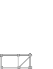
(a)	(b)

Figure 2. (a) An example of a domain $\Omega_{\varepsilon}$. The vertex parts are dark-shaded. (b) The associated one-dimensional skeleton $X$.

Denote by $-\Delta^{\Omega_{\varepsilon}}_{D}$ the Dirichlet Laplacian in $\Omega_{\varepsilon}$. In various applications, one is interested in the asymptotics of its eigenvalues $\lambda_{m}(-\Delta^{\Omega_{\varepsilon}}_{D})$ as $\varepsilon$ tends to $0$, see e.g. the monographs [11, 25] and the reviews [15, 17]. As the domain $\Omega_{\varepsilon}$ collapses onto it one-dimensional skeleton $X$ composed from the intervals $I_{j}$ coupled at the vertices, see Figure 2(b), one may expect that the eigenvalue asymptotics might be determined by some effective operator acting on the functions defined on $X$. The results obtained by several authors, see e.g. [14, 19], can be informally summarized as follows. Consider the star waveguides $\Lambda_{k}$ associated to each vertex as described above, the associated Dirichlet Laplacians $-\Delta^{\Lambda_{k}}_{D}$ and their discrete eigenvalues $\lambda_{j}(-\Delta^{\Lambda}_{D})$, $j\in\{1,\dots,N(\Lambda_{k})\}$, $k\in\{1,\dots,K\}$, then the bottom of the essential spectrum is exactly the first Dirichlet eigenvalue $\nu$ of the cross-section $\omega$, and the following holds as $\varepsilon$ tends to $0$: there exists $N\geq N(\Lambda_{1})+\dots+N(\Lambda_{K})$ such that

• for $m\in\{1,\dots,N\}$ there holds

  $$\lambda_{m}(-\Delta^{\Omega_{\varepsilon}}_{D})=\dfrac{a_{m}}{\varepsilon^{2}}+\mathcal{O}(e^{-c_{m}/\varepsilon})\text{ with $a_{m}\in(0,\nu]$ and $c_{m}>0$},$$

• for any $m\geq 1$ there holds

  $$\lambda_{N+m}(-\Delta^{\Omega_{\varepsilon}}_{D})=\dfrac{\nu}{\varepsilon^{2}}+\mu_{m}+\mathcal{O}(\varepsilon),$$

  where $\mu_{m}$ are the eigenvalues of the self-adjoint operator $L$ in $\bigoplus_{j=1}^{J}L^{2}(0,\ell_{j})$ acting as $(f_{j})\mapsto(-f^{\prime\prime}_{j})$ with suitable self-adjoint boundary conditions determined by the scattering matrices of $-\Delta^{\Lambda_{k}}_{D}$ at the energy $\nu$.

The operator $L$, which is the so-called quantum graph laplacian on $X$ [4, 25], represents the sought ”effective operator”, and the associated boundary conditions describe the way how the branches of the network interact through the vertices in the limit $\varepsilon\to 0$. An exact formulation, including the case of non-identical cross-sections, is presented in [14, Theorems 2 and 3], but is is quite complicated and needs a number of precise definitions, and finding the boundary conditions for $L$ is a non-trivial transcendental problem, but the whole construction admits an important particular case giving the following simple result, see [14, Section 8] and [19, Theorem 7]:

Proposition 1.

Assume that none of $\Lambda_{k}$ admits a threshold resonance, then:

• Denote $N:=N(\Lambda_{1})+\dots+N(\Lambda_{K})$ and let $a_{1},\dots,a_{N}$ be the eigenvalues $\lambda_{j}(-\Delta^{\Lambda_{k}}_{D})$, $j\in\{1,\dots,N(\Lambda_{k})\}$, $k\in\{1,\dots,K\}$, enumerated in the non-decreasing order, then for $m\in\{1,\dots,N\}$ there holds, with some $c_{m}>0$,

  $$\lambda_{m}(-\Delta^{\Omega_{\varepsilon}}_{D})=\dfrac{a_{m}}{\varepsilon^{2}}+\mathcal{O}(e^{-c_{m}/\varepsilon})\quad\text{as $\varepsilon$ tends to $0$},$$

• for any $m\geq 1$ there holds

  $$\lambda_{N+m}(-\Delta^{\Omega_{\varepsilon}}_{D})=\dfrac{\nu}{\varepsilon^{2}}+\mu_{m}+\mathcal{O}(\varepsilon)\quad\text{as $\varepsilon$ tends to $0$},$$

  where $\mu_{m}$ is the $m$th eigenvalue of $D_{1}\mathop{\oplus}\dots\oplus D_{J}$, with $D_{j}$ being the Dirichlet Laplacian on $(0,\ell_{j})$.

In other words, in the absence of threshold resonances the effective operator $L$ is decoupled. Numerous papers claimed that the assumptions of Proposition 1 are generically satisfied, i.e. are true for “almost any” star waveguide, which is supported by various analytical arguments, see e.g. [10, 14, 15, 19]. Nevertheless, there are only few results guaranteeing the non-existence of a threshold resonance for an explicitly given configuration. In fact, the only explicitly formulated condition we are aware of is the one appearing e.g. in [14, Theorem 25], which applies to the above star waveguide $\Lambda$:

Proposition 2.

Let $C$ be a center of $\Lambda$. Denote by $-\Delta^{C}_{DN}$ the Laplacian in $L^{2}(C)$ with the Dirichlet boundary condition at $\partial C\mathop{\cap}\partial\Lambda$ and with the Neumann boundary condition at the remaining part of the boundary (e.g. on the dash lines in Figure 1). If one has the strict inequality

$$\lambda_{1}(-\Delta^{C}_{DN})>\nu,$$ (2)

then $\Lambda$ has no threshold resonance.

Recall that, by the min-max principle, for any $j\in\{1,\dots,N(\Lambda)\}$ there holds

$$\lambda_{j}(-\Delta^{\Lambda}_{D})\geq\lambda_{j}(-\Delta^{C}_{DN}).$$ (3)

Therefore, in the situation of Proposition 2 the operator $-\Delta^{\Lambda}_{D}$ has no discrete eigenvalues, i.e. $N(\Lambda)=0$, and its spectrum is $[\nu,+\infty)$. In particular, if one has a network $\Omega_{\varepsilon}$ of the above type and such that the star waveguide associated with each vertex satisfies the assumptions of Proposition 2, then the result of Proposition 1 takes a simpler form, as one simply has $N=0$. One should remark that this particular case of Proposition 1 was initially proved in [24] in a direct way, without explicit link to the threshold resonances. The condition (2) is usually interpreted as the smallness of the center of the star waveguide with respect to the thickness of the branches. This situation is quite special, and it is generally expected that deformed waveguides of constant width have discrete eigenvalues [7, 12, 13, 18, 20].

Recently, some specific star waveguide configurations in two and three dimensions were studied in [2, 21, 22], and the absence of threshold resonances was shown. One should remark that, in all the cases considered, the condition (2) is not satisfied, and a non-empty discrete spectrum is present. The aim of the present paper is to state explicitly the main condition used in the constructions of [2, 21, 22] and then to show how it can be applied to the analysis of more general geometric configurations. Our main contribution is as follows:

Theorem 3.

Let $C$ be a center of $\Lambda$ and $-\Delta^{C}_{DN}$ be as in Proposition 2. If

$$\lambda_{N(\Lambda)+1}(-\Delta^{C}_{DN})>\nu,$$ (4)

then $\Lambda$ has no threshold resonance.

As noted above, Proposition 2 is a special case of Theorem 3 with $N(\Lambda)=0$. For further references, let us state explicitly another obvious but important corollary corresponding to $N(\Lambda)=1$, which is essentially the condition used in [2, 21, 22]:

Corollary 4.

If the discrete spectrum $-\Delta^{\Lambda}_{D}$ is non-empty and for some center $C$ one has $\lambda_{2}(-\Delta^{C}_{DN})>\nu$, then $-\Delta^{\Lambda}_{D}$ has a single discrete eigenvalue and no threshold resonance.

The proof of Theorem 3 is given in the following section, and it is quite elementary. We show first, using an explicit construction of test functions, that the presence of a threshold resonance gives rise to additional eigenvalues if one perturbs the Dirichlet Laplacian in $\Lambda$ by a negative potential. Then we show that such a behavior contradicts the assumption (4). In fact, a similar scheme was used in [21, 22] but with a different type of perturbation. Our choice of a potential perturbation allows for a more straightforward use of the min-max principle, and the resulting proof appears to be less technical.

In Section 3 we present several explicit examples in two and three dimensions in which the assumptions of Theorem 3 can be verified. Remark that the example given in subsection 3.5 is not covered by Corollary 4.

We remark at last that the Dirichlet boundary condition at the boundary of $\Lambda$ is only taken as an example, it can be replaced by some others such as Robin or mixed ones. Note that for the Neumann boundary condition one always has $\nu=0$, and there is a threshold resonance corresponding to the constant solutions of $-\Delta u=0$. In this case one always has $N(\Lambda)=0$, the operator $-\Delta^{C}_{DN}$ should be replaced by the Neumann Laplacian on $C$, whose first eigenvalue is $0=\nu$, and Eq. (4) is never satisfied.

2. Proof of Theorem 3

The proof is by assuming the opposite. We first show (Lemma 5) that if $\Lambda$ has a threshold resonance, then any perturbation of some class produces an additional eigenvalue, which is done by constructing a family of suitable test functions. On the other hand, in Lemma 8 we show that under the assumption (4) one can construct a perturbation of this class producing no new eigenvalues, which gives the result.

Recall that for a set $A$ we denote by $1_{A}$ its indicator function, which is defined by $1_{A}(x)=1$ for $x\in A$ and $1_{A}(x)=0$ otherwise.

2.1. Perturbations producing additional eigenvalues

This subsection is devoted to the proof of the following assertion.

Lemma 5.

Assume that $\Lambda$ has a threshold resonance. Let $\Omega\subset\Lambda$ be a non-empty bounded open set, then for any $\gamma>0$ the perturbed operator $-\Delta^{\Lambda}_{D}-\gamma 1_{\Omega}$ has at least $N(\Lambda)+1$ eigenvalues in $(-\infty,\nu)$.

The perturbation is compactly supported and does not change the essential spectrum, and by the min-max principle it is sufficient to find a $\big{(}N(\Lambda)+1\big{)}$-dimensional subspace $V\subset H^{1}_{0}(\Lambda)$ with

$$\sup_{v\in V\setminus\{0\}}\dfrac{\|\nabla v\|^{2}_{L^{2}(\Lambda)}-\gamma\|v\|^{2}_{L^{2}(\Omega)}}{\|v\|^{2}_{L^{2}(\Lambda)}}<\nu.$$ (5)

By assumption, there exists a non-zero bounded solution $u_{0}$ of (1). Denote for brevity $N:=N(\Lambda)$ and $\lambda_{j}:=\lambda_{j}(-\Delta^{\Lambda}_{D})$, $j\in\{1,\dots,N\}$, and choose an associated orthonormal family of eigenfunctions $u_{j}$ of $-\Delta^{\Lambda}_{D}$,

$$\langle u_{j},u_{k}\rangle_{L^{2}(\Lambda)}=\delta_{jk},\quad-\Delta u_{j}=\lambda_{j}u_{j},\quad j\in\{1,\dots,N\}.$$ (6)

Note that the functions $u_{0},\dots,u_{N}$ are smooth in $\Lambda$ due to the elliptic regularity. Let us emphasize another simple property:

Lemma 6.

The functions $u_{0},\dots,u_{N}$ are linearly independent on any non-empty open subset of $\Lambda$.

Proof.

Assume the opposite, i.e. that there exist a non-empty open subset $U\subset\Lambda$ and $\xi=(\xi_{0},\dots,\xi_{N})\in\mathbb{R}^{N+1}\setminus\{0\}$ such that

$$\sum\nolimits_{j=0}^{N}\xi_{j}u_{j}=0\text{ in }U.$$ (7)

Denote $\lambda_{0}:=\nu$ and $\Sigma:=\{\lambda_{0},\dots,\lambda_{N}\big{\}}$, pick any $\lambda\in\Sigma$ and apply successively the differential expressions $(-\Delta-\mu)$ with all $\mu\in\Sigma\setminus\{\lambda\}$ to Eq. (7). We arrive at

$$\Big{(}\prod_{\mu\in\Sigma\setminus\{\lambda\}}(\lambda-\mu)\Big{)}v_{\lambda}=0\text{ in }U,\quad v_{\lambda}:=\sum\nolimits_{j:\,\lambda_{j}=\lambda}\xi_{j}u_{j},$$

and the function $v_{\lambda}$ must vanish in $U$. On the other hand, it satisfies $-\Delta v_{\lambda}=\lambda v_{\lambda}$ in $\Lambda$, hence, $v_{\lambda}\equiv 0$ in $\Lambda$ due to the unique continuation principle. In particular, for $\lambda=\lambda_{0}=\nu$ we obtain $\xi_{0}u_{0}=0$ in $\Lambda$, and $\xi_{0}=0$ as $u_{0}$ is not identically zero. For $\lambda=\lambda_{k}$ with $k\neq 0$ we arrive at

$$\sum\nolimits_{j:\,\lambda_{j}=\lambda_{k}}\xi_{j}u_{j}=0\text{ in }\Lambda,$$

implying $\xi_{j}=0$ for all $j$ with $\lambda_{j}=\lambda_{k}$, as the family $(u_{1},\dots,u_{n})$ is orthonormal. Therefore, $\xi_{j}=0$ for all $j\in\{0,\dots,N\}$, which is in contradiction with $\xi\neq 0$. ∎

Let us pick a $C^{\infty}$ cut-off function $\chi:\mathbb{R}\to[0,1]$ with $\chi(r)=1$ for $r\leq 1$ and $\chi(r)=0$ for $r\geq 2$, and define $\varphi:\Lambda\to\mathbb{R}$ by $\varphi(x)=\chi\big{(}|x|/R\big{)}$ with some $R>R_{0}$, where $R_{0}$ is sufficiently large to have $\varphi=1$ on $\Omega$. Now set

$$v_{0}:=\varphi u_{0},\quad v_{j}=u_{j},\quad j\in\{1,\dots,N\}.$$

Lemma 7.

The functions $v_{0},\dots,v_{N}$ are linearly independent in $L^{2}(\Lambda)$ for any $R>R_{0}$.

Proof.

By construction, the functions are in $L^{2}(\Lambda)$. Furthermore, one has $v_{j}=u_{j}$ in $\Omega$ for $R>R_{0}$, and the result follows from Lemma 6. ∎

Now we are going to show the inequality (5) for $V:=\operatorname{span}(v_{0},\dots,v_{N})$ with a large $R$. It is sufficient to show that

$$\sup_{\xi\in\mathbb{R}^{n+1},\,|\xi|=1}\bigg{(}\Big{\|}\sum\nolimits_{j=0}^{N}\xi_{j}\nabla v_{j}\Big{\|}^{2}_{L^{2}(\Lambda)}-\nu\Big{\|}\sum\nolimits_{j=0}^{N}\xi_{j}v_{j}\Big{\|}^{2}_{L^{2}(\Lambda)}-\gamma\Big{\|}\sum\nolimits_{j=0}^{N}\xi_{j}v_{j}\Big{\|}^{2}_{L^{2}(\Omega)}\bigg{)}\\ \equiv\sup_{\xi\in\mathbb{R}^{n+1},\,|\xi|=1}\big{\langle}\xi,(A-\gamma B)\xi\big{\rangle}_{\mathbb{R}^{n+1}}<0,$$ (8)

with $A=(a_{jk})$, $B=(b_{jk})$,

$$a_{jk}:=\int_{\Lambda}\nabla v_{j}\cdot\nabla v_{k}\mathrm{d}x-\nu\int_{\Lambda}v_{j}v_{k}\mathrm{d}x,\quad b_{jk}:=\int_{\Omega}v_{j}v_{k}\mathrm{d}x,\quad j,k\in\{0,\dots,N\}.$$

More precisely, the coefficients of $A$ are

$$a_{00} =\int_{\Lambda}|\nabla(\varphi u_{0})\big{|}^{2}\,\mathrm{d}x-\nu\int_{\Lambda}(\varphi u_{0})^{2}\,\mathrm{d}x,$$

$$a_{j0} =a_{0j}=\int_{\Lambda}\nabla(\varphi u_{0})\cdot\nabla u_{j}\,\mathrm{d}x-\nu\int_{\Lambda}\varphi u_{0}u_{j}\,\mathrm{d}x,\quad j\in\{1,\dots,N\big{\}},$$

$$a_{jk} =(\lambda_{j}-\nu)\delta_{jk},\quad j,k\in\{1,\dots,N\big{\}}.$$

To estimate $a_{00}$ we remark that

$$\int_{\Lambda}|\nabla(\varphi u_{0})\big{|}^{2}\,\mathrm{d}x=\int_{\Lambda}|\nabla\varphi|^{2}u_{0}^{2}\,\mathrm{d}x+\int_{\Lambda}\varphi^{2}|\nabla u_{0}|^{2}\,\mathrm{d}x+2\int_{\Lambda}\varphi u_{0}\nabla\varphi\cdot\nabla u_{0}\,\mathrm{d}x,$$

and an integration by parts gives

$$2\int_{\Lambda}\varphi u_{0}\nabla\varphi\cdot\nabla u_{0}\,\mathrm{d}x=\int_{\Lambda}\nabla(\varphi^{2})\cdot\big{(}u_{0}\nabla u_{0})\,\mathrm{d}x=-\int_{\Lambda}\varphi^{2}\nabla\cdot(u_{0}\nabla u_{0})\,\mathrm{d}x\\ =-\int_{\Lambda}\varphi^{2}|\nabla u_{0}|^{2}\mathrm{d}x+\int_{\Lambda}\varphi^{2}(-\Delta u_{0})u_{0}\,\mathrm{d}x=-\int_{\Lambda}\varphi^{2}|\nabla u_{0}|^{2}\mathrm{d}x+\nu\int_{\Lambda}\varphi^{2}u_{0}^{2}\,\mathrm{d}x,$$

resulting in

$$a_{00}=\int_{\Lambda}|\nabla\varphi|^{2}u_{0}^{2}\,\mathrm{d}x.$$

For large $R$ there holds $\|\nabla\varphi\|_{\infty}\leq R^{-1}\|\chi^{\prime}\|_{\infty}=\mathcal{O}(R^{-1})$, and the volume of $\Lambda\mathop{\cap}\operatorname{supp}\nabla\varphi$ is $\mathcal{O}(R)$. Hence, due to the boundedness of $u_{0}$ there holds $a_{00}=\mathcal{O}(R^{-1})$ as $R\to+\infty$.

To estimate $a_{j0}$ with $j\neq 0$ we remark first that

$$\int_{\Lambda}\nabla(\varphi u_{0})\cdot\nabla u_{j}\,\mathrm{d}x =-\int_{\Lambda}\Delta(\varphi u_{0})u_{j}\,\mathrm{d}x$$

$$=\int_{\Lambda}(-\Delta\varphi)u_{0}u_{j}\,\mathrm{d}x-2\int(u_{j}\nabla\varphi)\cdot\nabla u_{0}\,\mathrm{d}x+\int_{\Lambda}\varphi(-\Delta u_{0})u_{j}\,\mathrm{d}x$$

$$=\int_{\Lambda}(-\Delta\varphi)u_{0}u_{j}\,\mathrm{d}x+2\int_{\Lambda}u_{0}\nabla\cdot(u_{j}\nabla\varphi)\,\mathrm{d}x+\nu\int_{\Lambda}\varphi u_{0}u_{j}\,\mathrm{d}x$$

$$=\int_{\Lambda}(\Delta\varphi)u_{0}u_{j}\,\mathrm{d}x+2\int_{\Lambda}u_{0}\nabla u_{j}\cdot\nabla\varphi\,\mathrm{d}x+\nu\int_{\Lambda}\varphi u_{0}u_{j}\,\mathrm{d}x,$$

hence,

$$a_{j0}=a_{0j}=\int_{\Lambda}(\Delta\varphi)u_{0}u_{j}\,\mathrm{d}x+2\int_{\Lambda}u_{0}\nabla u_{j}\cdot\nabla\varphi\,\mathrm{d}x.$$

We estimate, using the Cauchy-Schwarz inequality,

$$\bigg{|}\int_{\Lambda}u_{0}\nabla u_{j}\cdot\nabla\varphi\,\mathrm{d}x\bigg{|}\leq\int_{\Lambda}|\nabla u_{j}|\cdot|u_{0}\nabla\varphi|\,\mathrm{d}x\\ \leq\sqrt{\int_{\Lambda}|\nabla u_{j}|^{2}\,\mathrm{d}x}\cdot\sqrt{\int_{\Lambda}|\nabla\varphi|^{2}u_{0}^{2}\,\mathrm{d}x}=\mathcal{O}\Big{(}\dfrac{1}{\sqrt{R}}\Big{)},\quad R\to+\infty.$$

Due to

$$\Delta\varphi(x)=\dfrac{1}{R^{2}}\,\chi^{\prime\prime}\Big{(}\dfrac{|x|}{R}\Big{)}+\dfrac{d-1}{|x|}\,\dfrac{1}{R}\,\chi^{\prime}\Big{(}\dfrac{|x|}{R}\Big{)}$$

one has $\|\Delta\varphi\|_{\infty}=\mathcal{O}(R^{-1})$ for large $R$. At the same time, the volume of $\Lambda\mathop{\cap}\operatorname{supp}(\Delta\varphi)$ is $\mathcal{O}(R)$ and $u_{0}$ is bounded, therefore,

$$\bigg{|}\int_{\Lambda}(\Delta\varphi)u_{0}u_{j}\,\mathrm{d}x\bigg{|}\leq\sqrt{\int_{\Lambda}(\Delta\varphi)^{2}u_{0}^{2}\,\mathrm{d}x}\cdot\sqrt{\int_{\Lambda}u_{j}^{2}\,\mathrm{d}x}=\mathcal{O}\Big{(}\dfrac{1}{\sqrt{R}}\Big{)},$$

hence, $a_{j0}=a_{0j}=\mathcal{O}(R^{-\frac{1}{2}})$ as $R\to+\infty$ for $j\in\{1,\dots,N\big{\}}$, and,

$$A=\operatorname{diag}(0,\lambda_{1}-\nu,\dots,\lambda_{N}-\nu)+\mathcal{O}(R^{-\frac{1}{2}}),\quad R\to+\infty.$$

In particular, for a suitable $a>0$ there holds

$$\sup_{\xi\in\mathbb{R}^{n+1},\,|\xi|=1}\langle\xi,A\xi\rangle_{\mathbb{R}^{n+1}}\leq aR^{-\frac{1}{2}}\text{ for }R\to+\infty.$$ (9)

To estimate $B$ we remark that for $R>R_{0}$ one has $v_{j}=u_{j}$ in $\Omega$, and

$$b_{jk}=\int_{\Omega}u_{j}\,u_{k}\mathrm{d}x,\quad j,k\in\{0,\dots,N\}.$$

Hence, due to the compactness of the unit ball of $\mathbb{R}^{n+1}$ and to Lemma 6 there holds

$$\inf_{\xi\in\mathbb{R}^{n+1},\,|\xi|=1}\langle\xi,B\xi\rangle_{\mathbb{R}^{n+1}}=\inf_{\xi\in\mathbb{R}^{n+1},\,|\xi|=1}\Big{\|}\sum\nolimits_{j=0}^{N}\xi_{j}u_{j}\Big{\|}_{L^{2}(\Omega)}^{2}=:b>0.$$ (10)

The combination of (9) and (10) gives

$$\sup_{\xi\in\mathbb{R}^{n+1},\,|\xi|=1}\big{\langle}\xi,(A-\gamma B)\xi\big{\rangle}_{\mathbb{R}^{n+1}}\leq aR^{-\frac{1}{2}}-\gamma b<0\text{ for }R\to+\infty,$$

and the substitution into (8) concludes the proof.

2.2. Perturbations producing no eigenvalues

Lemma 8.

Assume that the inequality (4) is satisfied, then for sufficiently small $\gamma>0$ the operator $-\Delta^{\Lambda}_{D}-\gamma 1_{C}$ has exactly $N(\Lambda)$ eigenvalues in $(0,\nu)$.

Proof.

The perturbation potential is non-positive and with a compact support, hence, it does not change the essential spectrum and one has at least $N=N(\Lambda)$ eigenvalues in $(0,\nu)$. Assume that there exists an $(N+1)$th eigenvalue, then by the min-max principle it should satisfy $\lambda_{N+1}(-\Delta^{\Lambda}_{D}-\gamma 1_{C})\geq\lambda_{N+1}(A)$, where $A$ in the operator $-\Delta-\gamma 1_{C}$ in $L^{2}(\Lambda)$ with the Dirichlet boundary condition at $\partial\Lambda$ and an additional Neumann boundary condition at the both sides of $\partial C\mathop{\cap}\partial\Lambda$. The operator $A$ is unitarily equivalent to $(-\Delta^{C}_{DN}-\gamma)\oplus A_{1}\dots\oplus A_{n}$, where each $A_{j}$ is the Laplacian in $L^{2}(\mathbb{R}_{+}\times\omega_{j})$ with the Dirichlet boundary condition at $(\partial\omega_{j})\times\mathbb{R}_{+}$ and with the Neumann boundary condition at $\omega_{j}\times\{0\}$, and by the separation of variables one has $\operatorname{spec}(A_{j})=[\nu_{j},+\infty)$ and $A_{j}\geq\nu$. Therefore, $\lambda_{N+1}(A)=\lambda_{N+1}(-\Delta^{C}_{DN}-\gamma)=\lambda_{N+1}(-\Delta^{C}_{DN})-\gamma$, and $\lambda_{N+1}(-\Delta^{\Lambda}_{D}-\gamma 1_{C})\geq\lambda_{N+1}(-\Delta^{C}_{DN})-\gamma$. By (4), for sufficiently small $\gamma$ the right-hand side is still greater than $\nu$, while the left-hand side is strictly less than $\nu$, which is a contradiction. ∎

3. Examples

Due to a large number of possible examples, cf. [20], we restrict our attention to the configurations for which either a particularly explicit result or an improvement of previous studies can be presented.

3.1. Rounded corner

As one of the simplest examples one can consider the configuration $\Lambda$ consisting of two copies of the half-strip $\mathbb{R}_{+}\times(0,1)$ attached to the flat sides of a circular sector $C$ of unit radius and of opening $\alpha\in(0,\pi)$, see Figure 3(a). In the polar coordinates $(r,\theta)$ one has $C:=\big{\{}(r,\theta):r\in(0,1),\,\theta\in(0,\alpha)\big{\}}$. The cross-section is $\omega=(0,1)$ with $\nu=\pi^{2}$.

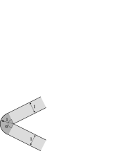
(a)

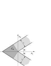
(b)

Figure 3. (a) Waveguide with a rounded corner. The center $C$ is dark-shaded. (b) Broken waveguide $\Lambda_{\alpha}$ with a dark-shaded center $C_{\alpha}$.

Proposition 9.

For any $\alpha\in(0,\pi)$, the operator $-\Delta^{\Lambda}_{D}$ has a single discrete eigenvalue and no threshold resonance.

Proof.

The existence of at least one eigenvalue follows from the general results for curved waveguides of constant width [13]. The associated operator $-\Delta^{C}_{DN}$ admits a separation of variables in polar coordinates, and the eigenvalues are the numbers $\lambda_{n,k}:=\big{(}j_{\frac{\pi n}{\alpha},k}\big{)}^{2}$, $n\in\mathbb{N}\mathop{\cup}\{0\}$, $k\in\mathbb{N}$, where $j_{s,k}$ is the $k$th zero of the Bessel function $J_{s}$. Recall, see e.g. [16], that we have the inequalities $j_{s,k}>s+k\pi-\frac{1}{2}$ for $s>\frac{1}{2}$ and $j_{s,k}>s+k\pi-\frac{\pi}{2}+\frac{1}{2}$ for $s>-\frac{1}{2}$, and it follows that $\lambda_{n,k}>\nu$ for $(n,k)\neq(0,1)$. As the lowest eigenvalue $\lambda_{0,1}$ is simple, the result follows by Corollary 4. ∎

3.2. Broken waveguide

Consider the domain

$$\Lambda_{\alpha}=\Big{\{}(x_{1},x_{2}):\dfrac{\cos\alpha}{\sin\alpha}\,|x_{2}|-\dfrac{1}{\sin\alpha}<x_{1}<\dfrac{\cos\alpha}{\sin\alpha}|x_{2}|\Big{\}},\quad\alpha\in\Big{(}0,\frac{\pi}{2}\Big{)}.$$

The domain can be considered as two copies of the half-strip $\mathbb{R}_{+}\times(0,1)$ attached to a quadrangle $C_{\alpha}$ having a symmetry axis, see Figure 3(b). As in the previous example, $\nu=\pi^{2}$. It is known since a long time, cf. [1], that the discrete spectrum is always non-empty, that each discrete eigenvalue is monotonically increasing with respect to $\alpha$, that the number of the eigenvalues increases infinitely as $\alpha$ approaches $0$, and the eigenvalue asymptotics for small $\alpha$ is computed in [9]. A very detailed discussion can be found in [8]. We would like to improve the existing results as follows.

Proposition 10.

For $\alpha\in\big{(}\arctan\frac{\sqrt{3}}{4},\frac{\pi}{2}\big{)}$ the operator $-\Delta^{\Lambda_{\alpha}}_{D}$ has a single discrete eigenvalue and no threshold resonance.

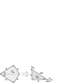
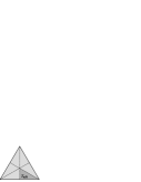
(a)	(b)

Figure 4. (a) The quadrangle $C_{\alpha}$ and the triangle $T_{\alpha}$. The symbols $D/N$ correspond to the Dirichlet/Neumann boundary condition. (b) The equilaterial triangle $\Omega$.

Proof.

In view of Corollary 4 it is sufficient to show that $\lambda_{2}(-\Delta^{C_{\alpha}}_{DN})>\pi^{2}$ for $\alpha$ in the interval indicated. The decomposition of $C_{\alpha}$ with respect to the horizontal symmetry axis shows that $-\Delta^{C_{\alpha}}_{DN}$ is unitarily equivalent to $A^{D}_{\alpha}\oplus A^{N}_{\alpha}$, where $A^{D/N}_{\alpha}$ are the Laplacians on the right-angled triangle $T_{\alpha}:=\big{\{}(x_{1},x_{1}):\,0<x_{2}<1-x_{1}\tan\alpha\big{\}}$ with the Dirichlet boundary condition on the bottom side, with the Neumann boundary condition on the left side and with the Dirichlet/Neumann boundary condition on the hypotenuse, see Figure 4(a). Denote

$$U:=\big{\{}u\in C^{\infty}(\overline{T_{\alpha}}):u(x_{1},x_{2})=0\text{ for $x_{1}=0$ or $x_{2}=1-x_{1}\tan\alpha$}\big{\}},$$

then $\lambda_{1}(A^{D}_{\alpha})=\inf_{u\in U\setminus\{0\}}\|\nabla u\|^{2}_{L^{2}(T_{\alpha})}/\|u\|^{2}_{L^{2}(T_{\alpha})}$. Furthermore, for $u\in U$ we have the one-dimensional inequalities

$$\int_{T_{\alpha}}\Big{(}\dfrac{\partial u}{\partial x_{1}}\Big{)}^{2}\mathrm{d}x =\int_{0}^{1}\int_{0}^{(1-x_{2})\cot\alpha}\Big{(}\dfrac{\partial u}{\partial x_{1}}\Big{)}^{2}\mathrm{d}x_{1}\,\mathrm{d}x_{2}$$

$$\geq\int_{0}^{1}\dfrac{\pi^{2}}{4(1-x_{2})^{2}\cot^{2}\alpha}\int_{0}^{(1-x_{2})\cot\alpha}u(x_{1},x_{2})^{2}\mathrm{d}x_{1}\,\mathrm{d}x_{2},$$

$$\int_{T_{\alpha}}\Big{(}\dfrac{\partial u}{\partial x_{2}}\Big{)}^{2}\mathrm{d}x =\int_{0}^{\cot\alpha}\int_{0}^{1-x_{1}\tan\alpha}\Big{(}\dfrac{\partial u}{\partial x_{2}}\Big{)}^{2}\mathrm{d}x_{2}\,\mathrm{d}x_{1}$$

$$\geq\int_{0}^{\cot\alpha}\dfrac{\pi^{2}}{(1-x_{1}\tan\alpha)^{2}}\int_{0}^{1-x_{1}\tan\alpha}u(x_{1},x_{2})^{2}\mathrm{d}x_{2}\,\mathrm{d}x_{1},$$

hence,

$$\|\nabla u\|^{2}_{L^{2}(T_{\alpha})}\geq\pi^{2}\int_{T_{\alpha}}\bigg{[}\dfrac{\tan^{2}\alpha}{4(1-x_{2})^{2}}+\dfrac{1}{(1-x_{1}\tan\alpha)^{2}}\bigg{]}\,u^{2}\,\mathrm{d}x\geq\pi^{2}\Big{(}\dfrac{1}{4}\,\tan^{2}\alpha+1\Big{)}\|u\|^{2}_{L^{2}(T_{\alpha})}.$$

Therefore, $A^{D}_{\alpha}>\pi^{2}$ for any $\alpha$, and it remains to find a condition guaranteeing that $\lambda_{2}(A^{N}_{\alpha})>\pi^{2}$.

Let us study now the operator $A^{N}_{\frac{\pi}{6}}$. Remark that any eigenfunction of $A^{N}_{\frac{\pi}{6}}$ can be extended, using the symmetries with respect to the Neumann sides, to a Dirichlet eigenfunction of the equilaterial triangle $\Omega$ with side length $2\sqrt{3}$, see Figure 4(b). Therefore, for any $k\in\mathbb{N}$ we have $\lambda_{k}(A^{N}_{\frac{\pi}{6}})\geq\lambda_{k}(-\Delta^{\Omega}_{D,s})$, where $-\Delta^{\Omega}_{D,s}$ is the restriction of the Dirichlet Laplacian $-\Delta^{\Omega}_{D}$ in $\Omega$ to the functions satisfying the Dirichlet boundary conditions, symmetric with respect to the medians and invariant under the rotations by $\frac{2\pi}{3}$ around the center of the triangle. Recall that the eigenvalues and the eigenfunctions of the Dirichlet Laplacian on the equilateral triangles are known explicitly, see e.g. [26], and the eigenvalues of $-\Delta^{\Omega}_{D}$ are the numbers

$$\mu_{m,n}=\dfrac{4\pi^{2}}{27}\big{(}m^{2}+mn+n^{2}),\quad(m,n)\in\mathbb{N}\times\mathbb{N}.$$

The eigenfunction corresponding to the first eigenvalue $\mu_{1,1}$ belongs to the domain of $-\Delta^{\Omega}_{D,s}$, hence, $\lambda_{1}(-\Delta^{\Omega}_{D,s})=\frac{4\pi^{2}}{9}$. On the other hand, one has $\lambda_{2}(-\Delta^{\Omega}_{D})=\lambda_{3}(-\Delta^{\Omega}_{D})=\mu_{1,2}\equiv\mu_{2,1}$, but no associated eigenfunction has the required symmetries: there is just one eigenfunction symmetric with respect to one of medians, but it is not rotationally invariant. Hence, $\lambda_{2}(A^{N}_{\pi/6})\geq\lambda_{2}(-\Delta^{\Omega}_{D,s})\geq\lambda_{4}(-\Delta^{\Omega}_{D})=\mu_{2,2}=\frac{16\pi^{2}}{9}>\pi^{2}$.

Note that the map $\Phi_{\alpha,\beta}:L^{2}(T_{\alpha})\to L^{2}(T_{\beta})$ given by

$$\big{(}\Phi_{\alpha,\beta}u\big{)}(x_{1},x_{2})=u\Big{(}\dfrac{\cot\alpha}{\cot\beta}x_{1},x_{2}\Big{)}$$

is bijective from the form domain of $A^{N}_{\alpha}$ to that of $A^{N}_{\beta}$, and

$$\dfrac{\|\nabla\Phi_{\alpha,\beta}u\|^{2}_{L^{2}(T_{\beta})}}{\|\Phi_{\alpha,\beta}u\|^{2}_{L^{2}(T_{\beta})}}=\dfrac{\displaystyle\int_{T_{\alpha}}\bigg{[}\Big{(}\dfrac{\tan\beta}{\tan\alpha}\Big{)}^{2}\Big{(}\dfrac{\partial u}{\partial x_{1}}\Big{)}^{2}+\Big{(}\dfrac{\partial u}{\partial x_{2}}\Big{)}^{2}\bigg{]}\mathrm{d}x}{\|u\|_{L^{2}(T_{\alpha})}},$$

and it follows by the min-max principle that

$$\lambda_{k}(A^{N}_{\beta})\geq\min\bigg{\{}\Big{(}\dfrac{\tan\beta}{\tan\alpha}\Big{)}^{2},1\bigg{\}}\lambda_{k}(A^{N}_{\alpha}),\quad\quad k\in\mathbb{N}.$$ (11)

Hence, for $\alpha\geq\frac{\pi}{6}$ we obtain $\lambda_{2}(A^{N}_{\alpha})\geq\lambda_{2}(A^{N}_{\frac{\pi}{6}})>\pi^{2}$, while for $\alpha<\frac{\pi}{6}$ we arrive at

$$\lambda_{2}(A^{N}_{\alpha})\geq\Big{(}\dfrac{\sqrt{3}}{\cot\alpha}\Big{)}^{2}\lambda_{2}(A^{N}_{\frac{\pi}{6}})=\dfrac{16\pi^{2}}{3}\,\tan^{2}\alpha,$$

and $\lambda_{2}(A^{N}_{\alpha})>\pi^{2}$ for $\tan\alpha>\frac{\sqrt{3}}{4}$. ∎

Remark that our lower bound $\arctan\frac{\sqrt{3}}{4}\simeq 0.409\simeq 23.4^{\circ}$ for the existence of a unique discrete eigenvalue improves the previously known value $\arctan\sqrt{0.4}\simeq 0.564\simeq 32.3^{\circ}$ obtained in [23]. Anyway, our estimate is not expected to be optimal: the numerical simulations [18, 23] suggest that the second eigenvalue appears for $\alpha\simeq 0.242\simeq 13.7^{\circ}$.

Note that in this specific example a more detailed result can obtained using the monotonicity of the eigenvalues with respect to the angle. Namely, denote $\mathcal{N}(\alpha):=N(\Lambda_{\alpha})$ the number of the discrete eigenvalues, the function $\mathcal{N}$ is then piecewise constant and non-increasing, and $\mathcal{N}(\alpha)$ tends to $\infty$ as $\alpha$ approaches $0$. Hence, there exists an infinite sequence $\frac{\pi}{2}=\alpha_{0}>\alpha_{1}>\alpha_{2}>\dots$ such that $\mathcal{N}$ is constant on each interval $[\alpha_{n},\alpha_{n-1})$ but has a jump at each $\alpha_{n}$, $n\in\mathbb{N}$, and $\alpha_{1}\leq\arctan\frac{\sqrt{3}}{4}$ by Proposition 10. A modification of the proof of Theorem 3 presented in Appendix A gives then the following result:

Proposition 11.

Assume that $\Lambda_{\alpha}$ admits a threshold resonance for some $\alpha\in\big{(}0,\frac{\pi}{2}\big{)}$, then the counting function $\mathcal{N}$ has a jump at $\alpha$.

In other words, there is just a discrete (but infinite) family of critical angles for which the existence of threshold resonances is possible. Remark that such a picture is typical for problems with threshold resonances, cf. [27], and it appears in other problems governed by geometric parameters, see e.g. [5, 6, 21].

3.3. T- and Y-junctions

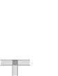
(a)

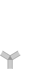
(b)

Figure 5. (a) $T$-shaped waveguide $\Lambda_{T}$. (b) $Y$-shaped waveguide $\Lambda_{Y}$.

The $T$-junction $\Lambda_{T}$ represents three copies of the half-strip $\mathbb{R}_{+}\times(0,1)$ attached to three sides of a unit square, while the $Y$-junction $\Lambda_{Y}$ is obtained from three copies of the same half-strip attached to the three sides of an equalateral triangle of unit side length, see Figure 5, and the absense of threshold resonances for the two configurations was already obtained in [21, 22]. For illustrative purposes, let us repeat the respective constructions. For the both cases we have $\nu=\pi^{2}$, and the presence of the discrete spectrum follows from the domain monotonicity by comparing with the broken waveguides (see subsection 3.2) with $\alpha=\frac{\pi}{4}$ for $\Lambda_{T}$ and $\alpha=\frac{\pi}{3}$ for $\Lambda_{Y}$. For $\Lambda_{T}$, the operator $-\Delta^{C}_{DN}$ is the Laplacian on the unit square with the Dirichlet boundary condition on one side and the Neumann boundary condition on the other three sides. The separation of variables shows that $\lambda_{2}(-\Delta^{C}_{DN})=\frac{5\pi^{2}}{4}>\nu$, and Corollary 4 gives the result. For $\Lambda_{Y}$, the operator $-\Delta^{C}_{DN}$ is the Neumann Laplacian in the equilateral triangle of unit side length, and its second eigenvalue is $\frac{16\pi^{2}}{9}>\nu$, see [26], and we are again in the situation of Corollary 4.

Using a construction similar to the one used in the proof of Proposition 10 one can consider a more general class of domains starting either with $\Lambda_{T}$ or with $\Lambda_{Y}$. Namely, for $\theta\in\mathbb{R}$ denote by $L_{\theta}$ the ray $\mathbb{R}_{+}(\cos\theta,\sin\theta)$. For $\alpha\in(0,\frac{\pi}{2}]$ consider the union of three rays $Y_{\alpha}:=L_{-\frac{\pi}{2}}\mathop{\cup}L_{\frac{\pi}{2}-\alpha}\mathop{\cup}L_{\frac{\pi}{2}+\alpha}$ and denote by $\Lambda_{Y,\alpha}$ its $\frac{1}{2}$-neighborhood, see Figure 6. Remark that for $\alpha=\frac{\pi}{3}$ and $\alpha=\frac{\pi}{2}$ we obtain respectively the above sets $\Lambda_{Y}$ and $\Lambda_{T}$.

Proposition 12.

Denote $\alpha_{1}:=\arccos(\sqrt{13}-3)\simeq 52,7^{\circ}$ and $\alpha_{2}:=\arctan\frac{4}{\sqrt{3}}\simeq 66,6^{\circ}$, then for $\alpha\in(\alpha_{1},\alpha_{2})$ the Dirichlet Laplacian in $\Lambda_{Y,\alpha}$ has a unique discrete eigenvalue and no threshold resonance.

Proof.

We are going to apply Corollary 4 again. The existence of a non-empty discrete spectrum follows again by comparing with the broken waveguides. To study the eigenvalues $\lambda_{2}(-\Delta^{C}_{DN})$ we distinguish between the cases $\alpha<\frac{\pi}{3}$ and $\alpha>\frac{\pi}{3}$.

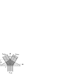
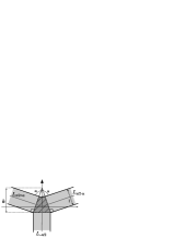
(a)	(b)

Figure 6. The domain $\Lambda_{Y,\alpha}$ for (a) $\alpha<\frac{\pi}{3}$ and (b) $\alpha>\frac{\pi}{3}$. The center $C$ is dark-shaded and the triangle $M$ is hatched.

Let $\alpha<\frac{\pi}{3}$, then the smallest possible center $C$ is a convex pentagon. By extending the three sides at which the Neumann boundary condition for $-\Delta^{C}_{DN}$ is imposed we obtain an isosceles triangle $M$ with the base length $l$ and the height $h$ given by

$$l=\dfrac{(2-\cos\alpha)\cos\alpha}{\sin^{2}\alpha},\quad h=\dfrac{2-\cos\alpha}{2\sin\alpha},$$

see Figure 6(a), and by the min-max principle we have the inequality $\lambda_{k}(-\Delta^{C}_{DN})\geq\lambda_{k}(-\Delta^{M}_{N})$, $k\in\mathbb{N}$, where $-\Delta^{M}_{N}$ is the Neumann Laplacian in $M$. Remark that $\frac{l}{h}=2\cot\alpha>\frac{2}{\sqrt{3}}$, while the last value is the base/height ratio for the equilateral triangles. Therefore, by applying the contraction with the coefficient $\sqrt{3}\cot\alpha$ along the $x_{1}$-axis we obtain an equilaterial triangle $\Omega$ of height $h$, and, similarly to (11), one has

$$\lambda_{k}(-\Delta^{M}_{N})\geq\Big{(}\dfrac{1}{\sqrt{3}\cot\alpha}\Big{)}^{2}\lambda_{k}(-\Delta^{\Omega}_{N}),\quad k\in\mathbb{N}.$$

As $\lambda_{2}(-\Delta^{\Omega}_{N})=\frac{4\pi^{2}}{3h^{2}}$, see [26], we arrive at

$$\lambda_{2}(-\Delta^{C}_{DN})\geq\dfrac{16\pi^{2}\sin^{4}\alpha}{9\cos^{2}\alpha(2-\cos\alpha)^{2}}=:\lambda(\alpha),$$

and solving the inequality $\lambda(\alpha)>\pi^{2}$ gives the sought lower bound for $\alpha$.

Now let $\alpha>\frac{\pi}{3}$, then the smallest possible center $C$ is a concave pentagon, and extending the Neumann sides one obtains an isosceles triangle $M$ with a unit base and the height $h=\frac{1}{2}\tan\alpha>\frac{\sqrt{3}}{2}$, and the contraction along the $x_{2}$ axis with the coefficient $\frac{1}{\sqrt{3}}\,\tan\alpha$ transforms $M$ into an equilateral triangle $\Omega_{0}$ of unit side length. As in (11) we have then

$$\lambda_{2}(-\Delta^{C}_{DN})\geq\lambda_{2}(-\Delta^{M}_{N})\geq\Big{(}\dfrac{\sqrt{3}}{\tan\alpha}\Big{)}^{2}\lambda_{2}(-\Delta^{\Omega_{0}}_{N})=\dfrac{16\pi^{2}}{3\tan^{2}\alpha},$$

and $\lambda_{2}(-\Delta^{C}_{DN})>\pi^{2}$ for $\tan\alpha<\frac{4}{\sqrt{3}}$, which gives the upper bound. ∎

3.4. Crossing strips

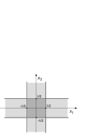
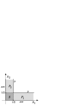
(a)	(b)

Figure 7. (a) The domain $\Lambda_{\times}$ with a dark-shaded center. (b) The domain $\Pi$ decomposed into the square $S$ and two half-infinite strips $P_{1}$ and $P_{2}$.

Consider the domain $\Lambda_{\times}:=\big{(}(-\frac{1}{2},\frac{1}{2})\times\mathbb{R}\big{)}\mathop{\cup}\big{(}\mathbb{R}\times(-\frac{1}{2},\frac{1}{2})\big{)}$, see Figure 7(a). It can be viewed as four copies on the half-infinite strip $(0,1)\times\mathbb{R}_{+}$ attached to the four sides of a unit square, and we have again $\nu=\pi^{2}$.

Proposition 13.

The Dirichlet Laplacian in $\Lambda_{\times}$ has a single discrete eigenvalue and no threshold resonance.

The rest of the subsection is dedicated to the proof. As in the preceding examples, the existence of discrete eigenvalues follows by comparing with broken waveguides. Remark that the operator $-\Delta^{C}_{DN}$ is simply the Neumann Laplacian on the unit square, and its second eigenvalue is $\pi^{2}=\nu$, and $-\Delta^{\Lambda}_{D}$ cannot have more than one discrete eigenvalue due to (3). On the other hand, as the strict inequality $\lambda_{2}(-\Delta^{C}_{DN})>\nu$ is not satisfied, the absence of threshold resonances does not follow directly from Corollary 4. We are going to show that the arguments can be modified in order to cover $\Lambda_{\times}$.

Assume by contradiction that there is a non-trivial bounded solution $w$ to $-\Delta w=\pi^{2}w$ in $\Lambda_{\times}$ vanishing at the boundary. For $j,k\in\{0,1\}$ consider the functions $w_{jk}$ defined by

$$w_{jk}(x_{1},x_{2})=w(x_{1},x_{2})+(-1)^{j}w(-x_{1},x_{2})+(-1)^{k}w(x_{1},-x_{2})+(-1)^{j+k}w(-x_{1},-x_{2}).$$

Each of these four functions is a bounded solution to $-\Delta u=\pi^{2}u$ in the domain $\Pi:=\big{(}(0,\frac{1}{2})\times\mathbb{R}_{+}\big{)}\mathop{\cup}\big{(}\mathbb{R}_{+}\times(0,\frac{1}{2})\big{)}$, see Figure 7(b), vanishing at $\partial\Lambda_{\times}\mathop{\cap}\partial\Pi$ and satisfying the following boundary conditions at the remaining part of the boundary:

$$(j,k)=(0,0): \text{ Neumann on }\{0\}\times\mathbb{R}_{+}\text{ and }\mathbb{R}_{+}\times\{0\},$$ (12)

$$(j,k)=(1,0): \text{ Dirichlet on }\{0\}\times\mathbb{R}_{+}\text{ and Neumann on }\mathbb{R}_{+}\times\{0\},$$

$$(j,k)=(0,1): \text{ Neumann on }\{0\}\times\mathbb{R}_{+}\text{ and Dirichlet on }\mathbb{R}_{+}\times\{0\},$$

$$(j,k)=(1,1): \text{ Dirichlet on }\{0\}\times\mathbb{R}_{+}\text{ and }\mathbb{R}_{+}\times\{0\}.$$

Furthermore, at least one of $w_{jk}$ is not identically zero. Let $A_{jk}$ be the Laplacian in $L^{2}(\Pi)$ with the Dirichlet boundary condition at $\partial\Lambda_{\times}\mathop{\cap}\partial\Pi$ and with the boundary conditions (12) on $\partial\Pi\setminus\partial\Lambda_{\times}$ and denote by $N_{jk}$ the number of discrete eigenvalues of $A_{jk}$ in $(0,\pi^{2})$. The Dirichlet Laplacian in $\Lambda_{\times}$ is then unitarily equivalent to the direct sum of $A_{jk}$, and one has $\sum_{j,k=0}^{1}N_{jk}=N(\Lambda_{\times})=1$. Proceeding literally as in Lemma 5 one proves the following assertion:

Lemma 14.

If $w_{jk}$ is not identically zero, then for any non-empty bounded open subset $\Omega$ of $\Pi$ and any $\gamma>0$ the operator $A_{jk}-\gamma 1_{\Omega}$ has at least $N_{jk}+1$ eigenvalues in $(0,\pi^{2})$.

In addition, denote by $A^{N}_{jk}$ the Laplacian in $L^{2}(\Pi)$ with the same boundary condition as $A_{jk}$ and an additional Neumann boundary condition at the lines $x_{1}=\frac{1}{2}$ and $x_{2}=\frac{1}{2}$, i.e. on the dash lines in Figure 7(b), then $A_{jk}\geq A^{N}_{jk}$. Furthermore, $A^{N}_{jk}=M^{0}_{jk}\oplus M^{1}_{jk}\oplus M^{2}_{jk}$, where $M^{0}_{jk}$, $M^{1}_{jk}$, $M^{2}_{jk}$ are Laplacians with suitable boundary conditions in respectively the square $S:=(0,\frac{1}{2})^{2}$ and the half-strips $P_{1}:=(\frac{1}{2},\infty)\times(0,\frac{1}{2})$ and $P_{2}:=(0,\frac{1}{2})\times(\frac{1}{2},\infty)$, and each $M^{s}_{jk}$ admits a separation of variables. Due to the inequality $A_{jk}-\gamma 1_{\Omega}\geq A^{N}_{jk}-\gamma 1_{\Omega}$ it is sufficient to construct, for each combination $(j,k)$, an non-empty bounded open set $\Omega_{jk}\subset\Pi$ such that

$$A^{N}_{jk}-\gamma 1_{\Omega_{jk}} N_{jk} (0,\pi^{2}) \gamma>0$$ has exactly eigenvalues in as is sufficiently small. (13)

Let $(j,k)=(1,1)$, then $M^{0}_{11}\geq 2\pi^{2}$, $M^{1}_{11}\simeq M^{2}_{11}\geq 4\pi^{2}$, and $A^{N}_{11}\geq 2\pi^{2}$, hence, $N_{11}=0$. Therefore, any $\Omega_{11}\subset\Pi$ satisfies (13). For $(j,k)=(1,0)$ we have $M^{0}_{10}\geq\pi^{2}$, $M^{1}_{10}\geq\pi^{2}$, $M^{2}_{10}\geq 4\pi^{2}$, $N_{10}=0$ and Eq. (13) is satisfied for any $\Omega_{10}\subset P_{2}$. In the same way, $N_{01}=0$, and Eq. (13) holds for $(j,k)=(0,1)$ with any $\Omega_{01}\subset P_{1}$. Finally, for $(j,k)=(0,0)$ we have $N_{11}=0$, $M^{1}_{00}\simeq M^{2}_{00}\geq\pi^{2}$ and $\lambda_{2}(M^{0}_{00})=4\pi^{2}>\pi^{2}$. Therefore, Eq. (13) holds with $\Omega_{00}=S$.

The combination of Lemma 14 with (13) gives Proposition 13.

3.5. Configuration with several discrete eigenvalues

The main difficulty in the use of Theorem 3 is that it requires the exact knowledge of the quantity $N(\Lambda)$. The analysis of the preceding examples was covered by Corollary 4 due to the equality $N(\Lambda)=1$. Let us give an example of a configuration $\Lambda$ with $N(\Lambda)=2$ for which the application of Theorem 3 is still possible.

For $a>0$ and $b>2$, denote $\Pi_{a,b}:=(0,a)\times(0,b)$. Let $\Lambda\equiv\Lambda_{a,b}$ be the star waveguide obtained by attaching two copies of the half-strip $\mathbb{R}_{+}\times(0,1)$ to a side of length $b$ of $\Pi_{a,b}$, see Figure 8(a). The exact position of the two branches along the side is not important, they are only assumed non-intersecting. We have obviously $\nu=\pi^{2}$.

Take as a center $C:=\Pi_{a,b}$. Let $A$ be the Laplacian in $\Pi_{a,b}$ with the Neumann boundary condition on a side of length $b$ and with the Dirichlet boundary conditions on the other three sides. Furthermore, let $B$ be the Dirichlet Laplacian in $\Pi_{a,b}$. Using the min-max principle we have then the following observations:

• if for some $j\in\mathbb{N}$ one has $\lambda_{j}(B)<\nu$, then $N(\Lambda)\geq j$,

• for any $j\in\big{\{}1,\dots,N(\Lambda)\big{\}}$ one has $\lambda_{j}(A)\leq\lambda_{j}(-\Delta^{\Lambda}_{D})\leq\lambda_{j}(B)$,

• for any $j\in\mathbb{N}$ one has $\lambda_{j}(A)\leq\lambda_{j}(-\Delta^{C}_{DN})$,

and a simple application of Theorem 3 gives the following assertion:

Lemma 15.

If for some $n\in\mathbb{N}$ one has the strict inequalities $\lambda_{n}(A)<\nu<\lambda_{n+1}(A)$ and $\lambda_{n}(B)<\nu$, then $N(\Lambda)=n$ and $\Lambda$ has no threshold resonance.

The operators $A$ and $B$ admit a separation of variables, and their eigenvalues are the numbers

$$\mu_{m,n}(A): =\pi^{2}\Big{(}\dfrac{(2m-1)^{2}}{4a^{2}}+\dfrac{n^{2}}{b^{2}}\Big{)}, m,n\in\mathbb{N},$$

$$\mu_{m,n}(B): =\pi^{2}\Big{(}\dfrac{m^{2}}{a^{2}}+\dfrac{n^{2}}{b^{2}}\Big{)}, m,n\in\mathbb{N},$$

respectively, enumerated in the non-decreasing order. Therefore, the following result holds:

Proposition 16.

Let $a$ and $b$ satisfy the inequalities

$$a>0,\quad b>2,\quad\dfrac{4}{a^{2}}+\dfrac{1}{b^{2}}<1<\dfrac{25}{4a^{2}}+\dfrac{1}{b^{2}},\quad 1<\dfrac{1}{4a^{2}}+\dfrac{4}{b^{2}},$$ (14)

then the Dirichlet Laplacian in $\Lambda$ has exactly two discrete eigenvalues and no threshold resonance.

Proof.

The inequalities (14) can be rewritten as $\mu_{2,1}(B)<\nu<\mu_{3,1}(A)$ and $\mu_{1,2}(A)>\nu$. As for $(j,k)\in\mathbb{N}\times\mathbb{N}$ there holds $\mu_{j,k}(A)<\mu_{j,k}(B)$, we arrive at $\lambda_{2}(A)=\mu_{2,1}(A)<\nu$ and $\lambda_{2}(B)=\mu_{2,1}(B)<\nu$ together with $\lambda_{3}(A)>\nu$, and the result follows from Lemma 15 with $n=2$. ∎

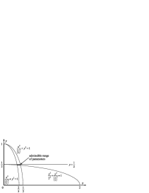
(a)	(b)

Figure 8. (a) The waveguide $\Lambda_{a,b}$. (b) The range of parameters $x=1/a$ and $y=1/b$ for which the assumptions of Proposition 16 are satisfied.

At last we remark that the set of $(a,b)$ given by (14) is non-empty. To see this, denote $x:=\frac{1}{a}$ and $y:=\frac{1}{b}$, then the conditions (14) read as

$$x>0,\quad 0<y<\dfrac{1}{2},\quad\dfrac{x^{2}}{\big{(}\frac{1}{2}\big{)}^{2}}+y^{2}<1<\dfrac{x^{2}}{\big{(}\frac{2}{5}\big{)}^{2}}+y^{2},\quad 1<\dfrac{x^{2}}{2^{2}}+\dfrac{y^{2}}{\big{(}\frac{1}{2}\big{)}^{2}},$$

and have a simple geometric representation, see Figure 8(b).

3.6. Three-dimensional configurations

The analysis of three dimensional domains is much harder due to a greater variety of possible shapes for both the cross-sections and the central domains, see e.g. [2, 20], so we just mention two examples.

The first one, $\Lambda_{\square}$, consists of three copies of half-infinite cylinders whose cross-section is a unit square attached to three mutually adjacent faces on a unit cube, see Figure 9(a). One has $\omega=(0,1)\times(0,1)$ with $\nu=2\pi^{2}$, and the existence of a non-empty discrete spectrum follows by the domain monotonicity from the comparison with $\Lambda_{\frac{\pi}{4}}\times(0,1)$, where $\Lambda_{\frac{\pi}{4}}$ is the broken waveguide of subsection 3.2. The associated operator $A_{\square}:=-\Delta^{C}_{DN}$ is the Laplacian in $(0,1)^{3}$ with the Dirichlet-Neumann combination of boundary conditions at each pair of opposite faces, and its second eigenvalue is $\frac{11\pi^{2}}{4}>2\pi^{2}=\nu$. Hence, Corollary 4 shows the existence of a unique discrete eigenvalue and the non-existence of a threshold resonance for $\Lambda_{\square}$.

The second configuration $\Lambda_{\mathrm{o}}$ consists of three half-infinite circular cylinders of radius $\frac{1}{2}$ attached to three mutually adjacent faces of a unit cube, see Figure 9(b). One has then $\nu=4j_{0,1}^{2}$ with $j_{0,1}\simeq 2.405$ being the first zero of the Bessel function $J_{0}$, i.e. $\nu\simeq 23.1$, and the existence of at least one discrete eigenvalue follows from the comparision with a sharply bent infinite cylinder of radius $\frac{1}{2}$ contained in $\Lambda_{\mathrm{o}}$, see [13]. The associated operator $-\Delta^{C}_{DN}$ can be minorated by the respective operator $A_{\square}$ from the previous example, hence, $\lambda_{2}(-\Delta^{C}_{DN})\geq\frac{11\pi^{2}}{4}\simeq 27.1>\nu$, and Corollary 4 shows that $\Lambda_{\mathrm{o}}$ has a single discrete eigenvalue and no threshold resonance.

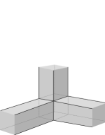
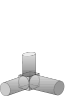
(a)	(b)

Figure 9. (a) The three-dimensional waveguide $\Lambda_{\square}$. (b) The three-dimensional waveguide $\Lambda_{\mathrm{o}}$.

In [2, 3], the intersection of two circular cylinders was considered, and the analysis was more involved. In particular, it was shown using an asymptotic estimate that the conditions of Corollary 4 are satisfied if one chooses a sufficiently big center.

Appendix A Proof of Proposition 11

Recall that the sesquilinear form for $-\Delta^{\Lambda_{\alpha}}_{D}$ is $q_{\alpha}(u,v)=\langle\nabla u,\nabla v\rangle_{L^{2}(\Lambda_{\alpha})}$, $u,v\in H^{1}_{0}(\Lambda_{\alpha})$. The domains $\Omega^{\pm}_{\alpha}:=\Lambda_{\alpha}\mathop{\cap}(\mathbb{R}\times\mathbb{R}_{\pm})$ are isometric to $\Pi_{\alpha}:=\big{\{}(s,t):\,t\in(0,1),\,s+t\cot\alpha>0\big{\}}$ using the representation

$$\Omega^{\pm}_{\alpha}=\big{\{}s\sigma^{\pm}_{\alpha}+t\tau^{\pm}_{\alpha}:(s,t)\in\Pi_{\alpha}\big{\}},\quad\sigma^{\pm}_{\alpha}:=(\cos\alpha,\pm\sin\alpha),\quad\tau^{\pm}_{\alpha}:=(-\sin\alpha,\pm\cos\alpha),$$

see Figure 10. For a function $u$ defined on $\Lambda_{\alpha}$ we denote by $u^{\pm}_{\alpha}$ the functions on $\Pi_{\alpha}$ defined by $u^{\pm}_{\alpha}(s,t)=u(s\sigma^{\pm}_{\alpha}+t\tau^{\pm}_{\alpha})$, $(s,t)\in\Pi_{\alpha}$, then

$$\|u\|^{2}_{L^{2}(\Lambda_{\alpha})} =\sum\nolimits_{\star\in\{+,-\}}\int_{\Pi_{\alpha}}u^{\star}_{\alpha}(s,t)^{2}\mathrm{d}s\,\mathrm{d}t,$$

$$q_{\alpha}(u,u) =\sum\nolimits_{\star\in\{+,-\}}\int_{\Pi_{\alpha}}\bigg{[}\Big{(}\dfrac{\partial u^{\star}_{\alpha}}{\partial s}(s,t)\Big{)}^{2}+\Big{(}\dfrac{\partial u^{\star}_{\alpha}}{\partial t}(s,t)\Big{)}^{2}\bigg{]}\mathrm{d}s\,\mathrm{d}t.$$ (15)

The linear map $\Phi_{\alpha,\beta}:L^{2}(\Lambda_{\alpha})\to L^{2}(\Lambda_{\beta})$ defined by

$$\big{(}\Phi_{\alpha,\beta}\big{)}^{\pm}_{\beta}(s,t)=\sqrt{\dfrac{\tan\beta}{\tan\alpha}}u^{\pm}_{\alpha}\Big{(}\dfrac{\tan\beta}{\tan\alpha}s,t\Big{)},\quad(s,t)\in\Pi_{\beta},$$

is unitary with $\Phi_{\alpha,\beta}\big{(}H^{1}_{0}(\Lambda_{\alpha})\big{)}=H^{1}_{0}(\Lambda_{\beta})$, and with the help of (15) one shows that for any $u,v\in H^{1}_{0}(\Lambda_{\alpha})$ there holds

$$q_{\beta}\big{(}\Phi_{\alpha,\beta}u,\Phi_{\alpha,\beta}v\big{)}=q_{\alpha}(u,v)+\bigg{(}\Big{(}\dfrac{\tan\beta}{\tan\alpha}\Big{)}^{2}-1\bigg{)}\sum\nolimits_{\star\in\{+,-\}}\int_{\Omega^{\star}_{\alpha}}(\sigma^{\star}_{\alpha}\cdot\nabla u\big{)}(\sigma^{\star}_{\alpha}\cdot\nabla v\big{)}\,\mathrm{d}x.$$ (16)

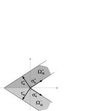
(a)	(b)

Figure 10. (a) Decomposition of $\Lambda_{\alpha}$ from subsection 3.2. (b) The set $\Pi_{\alpha}$.

Assume that $-\Delta^{\Lambda_{\alpha}}_{D}$ has exactly $n$ eigenvalues in $(-\infty,\pi^{2})$, to be denoted $\lambda_{1},\dots,\lambda_{n}$, and choose an associated orthonormal family of eigenfunctions of $-\Delta^{\Lambda_{\alpha}}_{D}$, i.e.

$$\langle u_{j},u_{k}\rangle_{L^{2}(\Lambda_{\alpha})}=\delta_{jk},\quad-\Delta u_{j}=\lambda_{j}u_{j},\quad j\in\{1,\dots,n\}.$$ (17)

Furthermore, by assumption there exists a non-zero bounded solution $u_{0}$ to (1) with $\Lambda=\Lambda_{\alpha}$.

Let $\beta\in(0,\alpha)$. Denote for shortness $\gamma:=1-\Big{(}\dfrac{\tan\beta}{\tan\alpha}\Big{)}^{2}>0$. We will show that $-\Delta^{\Lambda_{\beta}}_{D}$ has at least $n+1$ eigenvalues in $(-\infty,\pi^{2})$. By the min-max principle, it is sufficient to show that there exists a linearly independent family $(v_{0},\dots v_{n})\subset H^{1}_{0}(\Lambda_{\beta})$ such that

$$\sup_{\xi\in\mathbb{R}^{n+1},\,|\xi|=1}\langle\xi,M\xi\rangle_{\mathbb{R}^{n+1}}<0,$$ (18)

$$M=(m_{jk}),\quad m_{jk}=q_{\beta}(v_{j},v_{k})-\pi^{2}\langle v_{j},v_{k}\rangle_{L^{2}(\Lambda_{\beta})},\quad j,k\in\{0,\dots,n\big{\}}.$$

We construct such a family as follows. Let us pick a $C^{\infty}$ cut-off function $\chi:\mathbb{R}\to[0,1]$ with $\chi(r)=1$ for $r\leq 1$ and $\chi(r)=0$ for $r\geq 2$ and define $\varphi:\Lambda_{\alpha}\to\mathbb{R}$ by $\varphi(x)=\chi\big{(}x/|R|\big{)}$ with some $R>(\sin\alpha)^{-1}$, to be chosen later (the condition $R>(\sin\alpha)^{-1}$ ensures that support of $\varphi$ covers the “tip” on the domain), and set $v_{0}:=\Phi_{\alpha,\beta}(\varphi u_{0})$ and $v_{j}=\Phi_{\alpha,\beta}(u_{j})$ for $j\in\{1,\dots,n\}$. As $\Phi_{\alpha,\beta}$ is an isomorphism, it follows from Lemma 7 that $v_{0},\dots,v_{n}$ are linearly independent. Denote $B=(b_{jk})$ with

$$b_{jk}:=\sum\nolimits_{\star\in\{+,-\}}\int_{\Omega^{\star}_{\alpha}}\big{(}\sigma^{\star}_{\alpha}\cdot\nabla v_{j}\big{)}\big{(}\sigma^{\star}_{\alpha}\cdot\nabla v_{k}\big{)}\,\mathrm{d}x,\quad j,k\in\{0,\dots,n\big{\}},$$

then due to (16) we can represent $M=A-\gamma B$ with $A=(a_{jk})$ with $a_{jk}$ given by (2.1), and the estimates of Subsection 2.1 show that, with a suitable $a>0$,

$$\sup_{\xi\in\mathbb{R}^{n+1},\,|\xi|=1}\langle\xi,A\xi\rangle_{\mathbb{R}^{n+1}}\leq aR^{-\frac{1}{2}}\text{ for }R\to+\infty.$$ (19)

Let us show that

$$\text{there exists $b>0$ such that }\inf_{\xi\in\mathbb{R}^{n+1},\,|\xi|=1}\langle\xi,B\xi\rangle_{\mathbb{R}^{n+1}}\geq b\text{ for }R\to+\infty.$$ (20)

We remark first that for any $\xi=(\xi_{0},\dots,\xi_{n})\in\mathbb{R}^{n+1}$ there holds

$$\langle\xi,B\xi\rangle_{\mathbb{R}^{n+1}}=\sum\nolimits_{\star\in\{+,-\}}\int_{\Omega^{\star}_{\alpha}}\Big{(}\sigma^{\star}_{\alpha}\cdot\nabla(\xi_{0}\varphi u_{0}+\sum\limits_{j=1}^{n}\xi_{j}u_{j}\big{)}\Big{)}^{2}\,\mathrm{d}x.$$ (21)

Choose some $R_{0}>(\sin\alpha)^{-1}$ and denote $\Omega:=\Lambda_{\alpha}\mathop{\cap}\big{\{}x\in\mathbb{R}^{2}:|x|<R_{0}\big{\}}$. As the subintegral function in (21) is non-negative and $\varphi=1$ on $\Omega$ for $R\geq R_{0}$, we arrive at

$$\langle\xi,B\xi\rangle_{\mathbb{R}^{n+1}}\geq\sum\nolimits_{\star\in\{+,-\}}\int_{\Omega\mathop{\cap}\Omega^{\star}_{\alpha}}\bigg{(}\sigma^{\star}_{\alpha}\cdot\nabla\Big{(}\sum\nolimits_{j=0}^{n}\xi_{j}u_{j}\Big{)}\bigg{)}^{2}\,\mathrm{d}x=:I(\xi),$$

and to prove (10) it is sufficient to check that $\inf_{\xi\in\mathbb{R}^{n+1},\,|\xi|=1}I(\xi)>0$. Assume that the inequality is false, then due to the compactness of the unit ball of $\mathbb{R}^{n+1}$ there exists $\xi=(\xi_{0},\dots,\xi_{n})$ with $|\xi|=1$ such that $I(\xi)=0$. As the subintegral expression is non-negative, this implies

$$\sigma^{\pm}_{\alpha}\cdot\nabla\Big{(}\sum\nolimits_{j=0}^{n}\xi_{j}u_{j}\Big{)}=0\text{ in }\Omega\mathop{\cap}\Omega^{\pm}_{\alpha}.$$ (22)

As each $u_{j}$ is a (generalized) Laplacian eigenfunction, it is $C^{2}$ inside $\Lambda_{\alpha}$, and, due to (22),

$$\sum\nolimits_{j=0}^{n}\xi_{j}u_{j}(x)=\psi^{\pm}(\tau^{\pm}_{\alpha}\cdot x),\quad x\in\Omega\mathop{\cap}\Omega^{\pm}_{\alpha}$$

with some $C^{2}$ functions $\psi^{\pm}:(0,1)\to\mathbb{R}$. Furthermore, the function $w$ given by

$$w(x)=\psi^{\pm}(\tau^{\pm}_{\alpha}\cdot x)\text{ for }x\in\Omega\mathop{\cap}\Omega^{\pm}_{\alpha},$$

coincides with a linear combination of $u_{j}$ and, hence, extends to a $C^{2}$ function in $\Omega$. In particular,

$$w(x_{1},0-)=w(x_{1},0+),\quad\dfrac{\partial w}{\partial x_{2}}(x_{1},0-)=\dfrac{\partial w}{\partial x_{2}}(x_{1},0+),\quad x_{1}\in\big{(}-(\sin\alpha)^{-1},0\big{)},$$

which results in the the following conditions for $\psi^{\pm}$, valid for all $x_{1}\in\big{(}-(\sin\alpha)^{-1},0\big{)}$:

$$\psi^{-}(-x_{1}\sin\alpha)=\psi^{+}(-x_{1}\sin\alpha),\quad(-\cos\alpha)(\psi^{-})^{\prime}(-x_{1}\sin\alpha)=(\cos\alpha)(\psi^{+})^{\prime}(-x_{1}\sin\alpha).$$

The first condition shows that $\psi^{+}=\psi^{-}=:\psi$, and the second one implies that $\psi$ is constant. As the above-mentioned function $w$ satisfies the Dirichlet boundary conditions at $\partial\Omega\mathop{\cap}\partial\Lambda_{\alpha}$, we have $\psi\equiv 0$ and $\xi_{0}u_{0}+\dots+\xi_{j}u_{j}=0$ in $\Omega$, and $\xi=0$ by Lemma 6. This contradiction with $|\xi|=1$ shows the claim (20). Finally, the combination of (19) and (20) shows that the sought inequality (18) is valid for large $R$.

References

- [1] Y. Avishai, D. Bessis, B. G. Giraud, G. Mantica: Quantum bound states in open geometries. Phys. Rev. B 44 (1991) 8028–8034.
- [2] F. L. Bakharev, S. G. Matveenko, S. A. Nazarov: Spectra of three-dimensional cruciform and lattice quantum waveguides. Dokl. Math. 92 (2015) 514–518.
- [3] F. L. Bakharev, S. G. Matveenko, S. A. Nazarov: Discrete spectrum of -shaped waveguide. Algebra i Analiz 28 (2016) 58–71, in Russian. English version appears in St. Petersburg Math. J.
- [4] G. Berkolaiko, P. Kuchment: Introduction to quantum graphs. Math. Surv. Monogr., Vol. 186, Amer. Math. Soc., 2013.
- [5] D. Borisov, P. Exner, R. Gadyl’shin: Geometric coupling thresholds in a two-dimensional strip. J. Math. Phys. 43 (2002) 6265–6278.
- [6] D. Borisov, P. Exner, A. Golovina: Tunneling resonances in systems without a classical trapping. J. Math. Phys. 54 (2013) 012102.
- [7] W. Bulla, F. Gesztesy, W. Renger, B. Simon: Weakly coupled bound states in quantum waveguides. Proc. Amer. Math. Soc. 125 (1997) 1487–1495.
- [8] M. Dauge, Y. Lafranche, N. Raymond: Quantum waveguides with corners. ESAIM: Proc. 35 (2012) 14–45.
- [9] M. Dauge, N. Raymond: Plane waveguides with corners in the small angle limit. J. Math. Phys. 53 (2012) 123529.
- [10] G. F. Dell’Antonio, E. Costa: Effective Schrödinger dynamics on -thin Dirichlet waveguides via quantum graphs: I. Star-shaped graphs. J. Phys. A: Math. Theor. 43 (2010) 474014.
- [11] P. Exner, H. Kovařík: Quantum waveguides. Theor. Math. Phys., Vol. 22, Springer, 2015.
- [12] P. Exner, P. Šeba: Bound states in curved quantum waveguides. J. Math. Phys. 30 (1989) 2574–2580.
- [13] J. Goldstone, R. L. Jaffe: Bound states in twisting tubes. Phys. Rev. B 45 (1992) 14100–14107.
- [14] D. Grieser: Spectra of graph neighborhoods and scattering. Proc. London Math. Soc. 97 (2008) 718–752.
- [15] D. Grieser: Thin tubes in mathematical physics, global analysis and spectral geometry. In P. Exner, J. Keating, P. Kuchment, T. Sunada, and A. Teplyaev (Eds.): Analysis on graphs and its applications. Proc. Symp. Pure Math., Vol. 77, AMS, 2008, pages 565–594.
- [16] E. K. Ifantis, P. D. Siafarikas: A differential equation for the zeros of Bessel functions. Appl. Anal. 20 (1985) 269–281.
- [17] P. Kuchment: Graph models of wave propagation in thin structures. Waves Random Media 12 (2002) 1–24.
- [18] J. T. Londergan, J. P. Carini, D. P. Murdock: Binding and scattering in two-dimensional systems. Lect. Notes. Phys. Monogr., Vol. 60, Springer, 1999.
- [19] S. Molchanov, B. Vainberg: Scattering solutions in networks of thin fibers: small diameter asymptotics. Commun. Math. Phys. 273 (2007) 533–559.
- [20] S. A. Nazarov: Discrete spectrum of cranked, branching, and periodic waveguides. St. Petersburg Math. J. 23 (2012) 351–379.
- [21] S. A. Nazarov: Bounded solutions in a T-shaped waveguide and the spectral asymptotics of the Dirichlet ladder. Comput. Math. Math. Phys. 54 (2014) 1261–1279.
- [22] S. A. Nazarov, K. Ruotsalainen, P. Uusitalo: Asymptotics of the spectrum of the Dirichlet Laplacian on a thin carbon nano-structure. C. R. Mecanique 343 (2015) 360–364.
- [23] S. A. Nazarov, A. V. Shanin: Trapped modes in angular joints of waveguides. Appl. Anal. 93 (2014) 572–582.
- [24] O. Post: Branched quantum wave guides with Dirichlet boundary conditions: the decoupling case. J. Phys. A: Math. Gen. 38 (2005) 4917–4932.
- [25] O. Post: Spectral analysis of graph-like spaces. Lect. Notes Math., Vol. 2039, Springer, 2012.
- [26] M. Práger: Eigenvalues and eigenfunctions of the Laplace operator on an equilateral triangle. Appl. Math. 43 (1998) 311–320.
- [27] J. Rauch: Local decay of scattering solutions to Schrödinger’s equation. Comm. Math. Phys. 61 (1978) 149–168.