Hard photodisintegration of ${}^{3}\text{He}$ into a pd pair

Abstract

The recent measurements of high energy photodisintegration of a ${}^{3}\text{He}$ nucleus to a $pd$ pair at $90^{0}$ center of mass demonstrated an energy scaling consistent with the quark counting rule with an unprecedentedly large exponent of $s^{-17}$. To understand the underlying mechanism of this process, we extended the theoretical formalism of the hard rescattering mechanism (HRM) to calculate the $\gamma$ ³He$\rightarrow pd$ reaction. In HRM the incoming high energy photon strikes a quark from one of the nucleons in the target which subsequently undergoes hard rescattering with the quarks from the other nucleons, generating a hard two-body system in the final state of the reaction. Within the HRM we derived the parameter-free expression for the differential cross section of the reaction, which is expressed through the ³He$\rightarrow pd$ transition spectral function, the cross section of hard $pd\rightarrow pd$ scattering, and the effective charge of the quarks being interchanged during the hard rescattering process. The numerical estimates of all these factors resulted in the magnitude of the cross section, which is surprisingly in good agreement with the data.

I Introduction

The large momentum transfer photoproduction reactions with two-body breakup of the nucleus represent one of the testing grounds for nuclear quantum chromodynamics (QCD). The striking characteristics of these processes is the enormous value of invariant energy produced even at moderate incident beam energy. The invariant energy of the photoproduction reaction is $s=m_{T}^{2}+2E_{\gamma}m_{T}$, which shows that it grows for the nuclear target $A$ times faster than that of the proton target, where $m_{T}$ is the mass of the target and $E_{\gamma}$ is the incident photon energy. Considering large and fixed center-of-mass (cm) angles in two-body break-up reactions allows us to provide large momentum transfers $t\sim-\frac{s}{2}(1-cos\theta_{cm})$, thus satisfying conditions for hard QCD scattering.

Hard nuclear scattering, in which the energy-momentum transferred to the nucleus is much larger than the nucleon masses, is one of the best processes to probe quark degrees of freedom in the nucleus. In the hard scattering kinematic regime, we expect that only the minimal Fock components dominate in the wave function of the particles involved in the scattering. This expectation results in the prediction of the constituent (or quark) counting rule, according to which the energy dependence of two-body hard reaction is defined by the number of fundamental constituents participating in the reactionBF73 ; MMT72 .

If we consider a reaction of the type $a+b\rightarrow c+d$, according to constituent counting rule, the energy dependence of the hard process should scale as

$$\frac{d\sigma^{(ab\rightarrow cd)}}{dt}\sim\frac{1}{s^{n_{a}+n_{b}+n_{c}+n_{d}-2}},$$ (1)

where $n_{i},i=a,b,c,d$ represent the numbers of the fundamental fields associated with respective particles involved in the process. For example, if $a$ is a proton, $n_{a}$ will equal 3, and if it is a photon, $n_{a}$ would be 1.

Even though the energy dependencies (or scaling relations) of Eq. (1) do not imply the onset of the perturbative QCD regime, they indicate that the resolution of the probe is such that it allows us to identify the constituents of the hadrons that participate in the hard scattering. In 1976 it was suggestedBC76 to use the concept of the quark-counting rule to explore the QCD degrees of freedom in nuclei. One of the best candidate reactions was hard photodisintegration of the deuteron, $\gamma+d\rightarrow p+n$, which, according to Eq. (1), should scale as $d\sigma/dt\sim s^{-11}$. The first such experiments being carried out at SLACNapolitano:1988uu ; Freedman:1993nt ; Belz:1995ge and Jefferson LabBochna:1998ca ; Schulte01se ; Schulte:2002tx ; Mirazita:2004rb ; Rossi:2004qm revealed $s^{-11}$ scaling for photon energies already at $E_{\gamma}\geq 1$ GeV and $\theta_{cm}=90^{o}$. It is worth mentioning that the calculations based on a conventional mesonic picture of strong interaction failed to explain the observed energy scaling, which can be considered another indication that the quark degrees of freedom need to be included for an adequate description of the reaction. The deuteron two-body hard photodisintegration reactions have been used also to measure the polarization observablesWijesooriya:2001yu ; Adamian:2000qc ; Jiang:2007ge ; Zachariou:2015clw , which were in general agreement with the quark-constituent picture of hard scattering.

To check the universality of the constituent counting rule for other hard breakup reactions, the two-body reactions were extended to a ³He target, in which case two fast outgoing protons and slow neutron were detected in the $\gamma+^{3}$He$\rightarrow(pp)+n$ reactiontgheppn2004 . The results of this experimentPomerantz:2009sb were consistent with the $s^{-11}$ scaling in the two-proton hard beak up channel, but at much larger photon energies ($E_{\gamma}>2$ GeV) than in the case of $pn$ breakup. Recently the hard two-body breakup reaction was measured for the more complex $\gamma+$ ³He$\rightarrow p+d$ channelPomerantz13 . According to Eq. (1) such a reaction in the hard scattering regime should scale as $s^{-17}$, and surprisingly the experiment observed a scaling consistent with the exponent of 17, an unprecedented large number to be observed in two-body hard processes.

In the present work, we extend the theoretical framework referred as hard rescattering mechanism(HRM) to calculate the cross section of above mentioned $\gamma^{3}$He$\rightarrow pd$ reaction. The HRM model was originally developed for calculation of $\gamma d\rightarrow pn$ reactionsgdpn . The model was successful not only in verifying the $s^{-11}$ dependence but also reproducing the absolute magnitude of the $\gamma+d\rightarrow pn$ cross sections without free parameters at $\gtrsim 1$ GeV incoming photon energies and large center of mass anglesgdpn ; gdpn2 ; gdpnang . The HRM model allowed also the calculation of polarization observables for the $\gamma d\rightarrow pn$ reactiongpdnpol , and its prediction for the large magnitude of transferred polarization was confirmed by the experiment of Ref.Jiang:2007ge . Subsequently the HRM model was applied to the $\gamma+^{3}$He $\rightarrow pp+n$ reactionsgheppn , in which two protons were produced in the hard break-up process while the neutron was soft. The model described the scaling properties and the cross section reasonably well and was able to explain the observed smaller cross section as compared to the deuteron break-up reaction. In Ref.gdBB it was shown also that HRM model can be extended to the hard break-up of the nucleus to any two-baryonic state which can be produced from the $NN$ scattering through the quark-interchange interaction. In the HRM model, a quark of the one nucleon knocked out by the incoming photon rescatters with a quark of the other nucleon leading to a production of two nucleons with large relative momentum. We assume in HRM that the quark interchange is the dominant mechanism for the hard rescattering of two outgoing energetic nucleons. The latter assumption is essential for factorization of the hard scattering kernel from the soft incalculable part of the scattering amplitude.

In the present work we apply a similar rescattering scenario for the hard break-up of a ³He nucleus to a $pd$ pair. Our main goal is to check whether the HRM approach, which explicitly accounts for the quark degrees of freedom, will allow us to reproduce the energy and angular dependencies of the measured cross sections. The article is organized as follows: Sec. II describes the kinematics and the reference frame of the two-body break-up reaction. In Sec. III, we develop the hard rescattering model for the $\gamma+^{3}$He$\rightarrow p+d$ reaction, discussing in detail the nuclear amplitude which according to HRM provides the main contribution to the hard break-up cross section. In Sec. IV we complete the derivation by calculating the cross section and considering the methods of estimation of nuclear and $pd\rightarrow pd$ rescattering parts entering in the cross section. Section IV presents numerical estimates and a comparison with the results of the recent experiments at $\theta_{cm}=90^{0}$. It also gives predictions for the angular distribution of the cross section as well as energy dependencies for other $\theta_{cm}$. Section V summarizes our results. In Appendix A, we present the details of the derivation discussed in the Sec. III. The discussion of the hard elastic $pd\rightarrow pd$ scattering is presented in Appendix B. Appendix C discusses the relationship between the light-front and non-relativistic ³He to deuteron transition wave functions.

II Kinematics of the Process and the Reference Frame

We are considering the following two-body photodisintegration reaction:

$$\gamma+^{3}\text{He}\rightarrow p+d,$$ (2)

where the proton and deuteron are produced at large angles measured in the center-of-mass reference frame of the reaction. The invariant energy $s$ and momentum transfer $t$ of the reaction are defined as

$$s = (q+p_{{}^{3}\text{He}})^{2}=m_{{}^{3}\text{He}}^{2}+2q\cdot p_{{}^{3}\text{He}}=m_{{}^{3}\text{He}}^{2}+2E_{\gamma}m_{{}^{3}\text{He}}=(E^{cm}_{\gamma}+E^{cm}_{{}^{3}\text{He}})^{2}$$

$$t = (q-p_{p})^{2}=m_{p}^{2}-2q\cdot p_{p}=m_{p}^{2}-2E_{\gamma}^{cm}(E_{p}^{cm}-p_{p}^{cm}\cos\theta_{cm}),$$ (3)

where $m_{p}$ and $m_{{}^{3}\text{He}}$ are masses of the proton and ³He target, respectively, and $E_{\gamma}$ is the incoming photon energy in the laboratory system. The four-vectors $q$, $p_{{}^{3}\text{He}}$, and $p_{p}$ define the four-momenta of photon, ³He, and proton respectively. In the right hand side of Eq. (3), we expressed $s$ and $t$ through the center-of-mass energies, momenta, and scattering angles of interacting particles defined as

$$E_{\gamma}^{cm} = \frac{1}{2\sqrt{s}}\big{(}s-m_{{}^{3}\text{He}}^{2}\big{)}\texttt{,}\ \ \ \ \ \ \ \ E_{{}^{3}\text{He}}=\frac{1}{2\sqrt{s}}\big{(}s+m_{{}^{3}\text{He}}^{2}\big{)}$$

$$E_{p}^{cm} = \frac{1}{2\sqrt{s}}\Big{(}s+m_{p}^{2}-m_{d}^{2}\Big{)}\texttt{,}\ \ E_{d}^{cm}=\frac{1}{2\sqrt{s}}\Big{(}s+m_{d}^{2}-m_{p}^{2}\Big{)}.$$ (4)

The one interesting property of Eq. (3), observed in Ref.Holt , is the possibility to generate large center-of-mass energy $s$ with moderate energy of photon beams. This is due to the fact that, in the expression of $s$, photon energy is multiplied by the mass of the target. For the case of reaction (2), for example, the photon energy, $E_{\gamma}=1$ GeV will generate $s$ as large as that generated by a $6$ GeV/$c$ proton beam in $pp$ scattering. This property was one of the reasons why the quark-counting scaling was observed in the $\gamma d\rightarrow pn$ reaction for photon energies as low as $1.2$ GeV at cm $90^{0}$ break-up kinematicsMirazita:2004rb ; Rossi:2004qm .

Using Eq. (4) in the expression for $t$ in Eq. (3), we obtain

$$t=m_{p}^{2}-\frac{1}{2s}(s-m_{{}^{3}\text{He}}^{2})\Big{[}(s+m_{p}^{2}-m_{d}^{2})-\sqrt{\left\{s-(m_{p}+m_{d})^{2}\right\}\left\{s-(m_{p}-m_{d})^{2}\right\}}\cos\theta_{cm}\Big{]}.$$ (5)

It follows from the above relation that in the high energy limit $t\sim-\frac{s}{2}(1-cos\theta_{cm})$, which indicates that at large and fixed values of $\theta_{cm}$ one can achieve the hard scattering regime, $-t(-u)\gg m_{N}^{2}$, providing large values of $s$. For the latter, it follows from the expression of $s$ in Eq. (3) that the photon energy $E_{\gamma}$ is multiplied by $2m_{{}^{3}\text{He}}$, because of which, even for moderate value of $E_{\gamma}$, the high energy condition ($s\gg m_{N}^{2}$) is easily achieved. This is seen in Fig. 1(a), where the invariant momentum transfer $-t$ is presented as a function of incoming photon energy $E_{\gamma}$ at large and fixed values of $\theta_{cm}$. As the figure shows, even at $E_{\gamma}\sim 1$ GeV the invariant momentum transfer $-t\sim 1$ (GeV/c)², which is sufficiently large for the reaction to be considered hard.

(a)

(b)

Figure 1: (a) Photon energy dependence of invariant momentum transfer $-t$. (b)Laboratory momenta of outgoing proton and deuteron as a function of photon energy. Solid lines denote proton, dashed lines denote deuteron. Calculations are done for $\theta_{cm}=90^{o}$ and $60^{o}$.

That the reaction (2) at $E_{\gamma}\gtrsim 1$ GeV and $\theta_{cm}\sim 90^{0}$ cannot be considered a conventional nuclear process with knocked-out nucleon and recoiled residual nuclear system follows from Fig.1(b), where the laboratory momenta of outgoing proton and deuteron are given for large $\theta_{cm}$. In this case, one observes that starting at $E_{\gamma}>1$ GeV/$c$ the momenta of outgoing proton and deuteron $>1$GeV/$c$. Such a large momentum of the deuteron significantly exceeds the characteristic Fermi momentum in the ³He nucleus, thus the deuteron cannot be considered residual. The momenta of the deuteron are also out of the kinematic range of eikonal, small-angle rescatteringgea ; ms01 ; noredepn , further diminishing the possibility of describing reaction (2) within the framework of conventional nuclear scattering.

Finally, another important feature of the large center-of-mass breakup kinematics is the early onset of QCD degrees of freedom due to the large inelasticities (or large masses) produced in the intermediate state of the reaction. As shown in Ref.GilmanGross for photodisinegration of the deuteron, already at photon energies of 1 GeV one needs around 15 channels of resonances in the intermediate state to describe the process within the hadronic approach. This situation is similar in the case of the ³He target, in which one estimates the produced mass of the intermediate state as $m_{R}\approx\sqrt{s}-M_{d}$. From this relation one observes that already at $E_{\gamma}=1$ GeV, $m_{R}\approx 1.8$ GeV, which is close to the deep inelastic threshold of $2$ GeV, for which QCD degrees of freedom are more adequate.

Overall, the above kinematical discussion gives justification for the theoretical description based on the QCD degrees of freedom to be increasingly valid starting at photon energies of $\sim 1$ GeV.

To conclude the section, we define the reference frame in which the reaction (2) will be considered. It is defined from the condition for the “+” and transverse components of incoming photon, $q^{+}=q_{\perp}=0$, with the photon and target nucleus having the following light-cone four-momenta:

$$q^{\mu} = (q_{+},q_{-},q_{\perp})=(0,\sqrt{s^{\prime}_{{}^{3}\text{He}}},0)$$

$$p^{\mu}_{{}^{3}\text{He}} = (p_{{}^{3}\text{He}+},p_{{}^{3}\text{He}-},p_{{}^{3}\text{He}\perp})=(\sqrt{s^{\prime}_{{}^{3}\text{He}}},\frac{m_{{}^{3}\text{He}}^{2}}{\sqrt{s^{\prime}_{{}^{3}\text{He}}}},0),$$ (6)

where $s^{\prime}_{{}^{3}\text{He}}=s-m_{{}^{3}\text{He}}^{2}$. In the above expression the $\pm$ components are defined as $p_{\pm}=E\pm p_{z}$, where the direction of $z$ axis is opposite to the momentum of the incoming photon in the laboratory frame.

III Hard Rescattering Mechanism

In the HRM model, the hard photodisintegration takes place in two stages. First, the incoming photon knocks out a quark from one of the nucleons. Then in the second step the outgoing fast quark undergoes a high momentum transfer hard scattering with the quark of the other nucleon sharing its large momentum among the constituents in the final state of the reaction. Since HRM utilizes the small momentum part of the target wave function, which has a large component of the initial $pd$ state, it is assumed that the energetic photon is absorbed by any of the quarks belonging to the protons in the nucleus, with the subsequent hard rescattering of struck quarks off the quarks in the “initial” $d$ system producing the final $pd$ state. Within such a scenario, the total scattering amplitude can be expressed as a sum of the multitude of the diagrams similar to that of Fig. 2, with all possibilities of struck and rescattered quarks combining into a fast outgoing $pd$ system. Instead of summing all the possible diagrams, the idea of HRM is to factorize the hard $\gamma q$ scattering and sum the remaining parts to the amplitude of hard elastic $pd\rightarrow pd$ scattering. In this way the complexities related to the large number of diagrams and nonperturbative quark wave function of the nucleons are absorbed into the $pd\rightarrow pd$ amplitude, which can be taken from experiment.

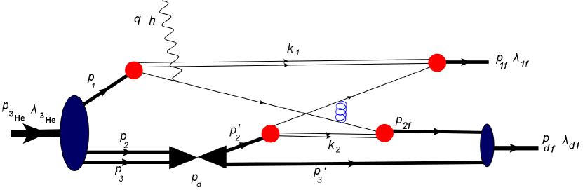
Figure 2: Typical diagram of hard rescattering mechanism of the $\gamma^{3}\text{He}\rightarrow pd$ reaction.

To demonstrate the above described concept of HRM, we consider the typical scattering diagram of Fig. 2. Here, the incoming photon knocks out a quark from one of the protons in the nucleus. The struck quark that now carries almost the whole momentum of the photon will share its momentum with a quark from the other nucleons through the quark interchange. The resulting two energetic quarks will recombine with the residual quark-gluon systems to produce a proton and deuteron with large relative momentum. Note that the assumption that the nuclear spectator system is represented by intermediate deuteron state is justified based on our previous studies of HRMgdpn ; gheppn , in which it was found that the scattering amplitude is dominated by small initial momenta of interacting nucleons. For the case of reaction Eq. (2), because of the presence of the deuteron in the final state, the small momentum of the initial proton in the ${}^{3}\text{He}$ nucleus will originate predominantly from a two-body $pd$ state.

In Fig. 2, $h$, $\lambda_{{}^{3}\text{He}},\lambda_{1f}\text{ and }\lambda_{df}$ are the helicities of the incoming photon, ${}^{3}\text{He}$ nucleus, and outgoing proton and deuteron respectively. Similarly, $q$, $p_{{}^{3}\text{He}},p_{1},p_{1f},p_{d}\text{ and }p_{df}$ are the momenta of the photon, ${}^{3}\text{He}$ nucleus, initial and outgoing protons, intermediate deuteron, and the final deuteron respectively. The $k$’s define the momenta of the spectator quark systems. The four-momenta defined in Fig. 2 satisfy the following relations:

$$p_{{}^{3}\text{He}}=p_{1}+p_{2}+p_{3};\quad p_{2}+p_{3}=p_{d}=p_{2}^{\prime}+p_{3}^{\prime};\quad p_{2f}+p_{3}^{\prime}=p_{df};\quad p_{{}^{3}\text{He}}+q=p_{1f}+p_{df},$$

where $p_{2}$, $p_{3}$, $p_{2}^{\prime}$ and $p_{3}^{\prime}$ are four-momenta of the nucleons in the intermediate state deuteron.

We now write the Feynman amplitude corresponding to the diagram of Fig. 2, identifying terms corresponding to nuclear and nucleonic parts as follows:

$$\mathcal{M}^{\lambda_{df},\lambda_{1f};\lambda_{{}^{3}\text{He}},h}=\sum_{\lambda_{d}^{\prime}}\int\chi_{d}^{*\lambda_{d}^{\prime}}(-i\Gamma_{{}_{DNN}}^{\dagger})\frac{i(\not{p}_{2f}+m)}{p_{2f}^{2}-m_{N}^{2}+i\epsilon}\frac{i(\not{p}_{3}^{\prime}+m)}{p_{3}^{\prime 2}-m_{N}^{2}+i\epsilon}\frac{i(\not{p}_{2}^{\prime}+m)}{p_{2}^{\prime 2}-m_{N}^{2}+i\epsilon}$$

$$A:\qquad i\frac{\Gamma_{{}_{DNN}}\chi_{d}^{\lambda_{d}}\chi_{d}^{*\lambda_{d}}}{p_{d}^{2}-m_{{}_{d}}^{2}+i\epsilon}(-i)\Gamma_{{}_{DNN}}^{\dagger}\frac{i(\not{p}_{3}+m)}{p_{3}^{2}-m_{N}^{2}+i\epsilon}\frac{i(\not{p}_{2}+m)}{p_{2}^{2}-m_{N}^{2}+i\epsilon}\frac{i(\not{p}_{1}+m)}{p_{1}^{2}-m_{N}^{2}+i\epsilon}$$

$$\qquad i\Gamma_{{}_{{}^{3}\text{He}}}\chi_{{}_{{}^{3}\text{He}}}^{\lambda_{{}^{3}\text{He}}}\dfrac{d^{4}p_{2}^{\prime}}{(2\pi)^{4}}\dfrac{d^{4}p_{3}}{(2\pi)^{4}}\dfrac{d^{4}p_{3}^{\prime}}{(2\pi)^{4}}$$

$$N1:\int\chi_{p_{1f}}(-i)\Gamma_{N1}^{\dagger}\frac{i(\not{p}_{1f}-\not{k}_{1}+m)}{(p_{1f}-k_{1})^{2}-m_{q}^{2}+i\epsilon}\Big{[}-igT_{c}^{\beta}\gamma_{\mu}\Big{]}\frac{iS(k_{1})}{k_{1}^{2}-m_{s}^{2}+i\epsilon}$$

$$\qquad\frac{i(\not{p}_{1}-\not{k}_{1}+m_{q})}{(p_{1}-k_{1})^{2}-m_{q}^{2}+i\epsilon}i\Gamma_{n1}\dfrac{d^{4}k_{1}}{(2\pi)^{4}}$$

$$N2:\int(-i)\Gamma_{N}^{\dagger}\frac{i(\not{p}_{2f}-\not{k}_{2}+m_{q})}{(p_{2f}-k_{2})^{2}-m_{q}^{2}+i\epsilon}\frac{iS(k_{2})}{k_{2}^{2}-m_{s}^{2}+i\epsilon}\frac{i(\not{p}_{2}^{\prime}-\not{k}_{2}+m_{q})}{(p_{2}^{\prime}-k_{2})^{2}-m_{q}^{2}+i\epsilon}i\Gamma_{n2^{\prime}}\dfrac{d^{4}k_{2}}{(2\pi)^{4}}$$

$$\gamma:-igT_{c}^{\alpha}\gamma_{\nu}\frac{i(\not{p}_{1}+\not{q}-\not{k_{1}}+m_{q})}{(p_{1}-k_{1}+q)^{2}-m_{q}^{2}+i\epsilon}\Big{[}-ie\gamma^{\mu}\epsilon^{\mu}_{h}\Big{]}$$

$$g:\frac{id_{\mu\nu}\delta_{\alpha\beta}}{q_{q}^{2}}.$$ (7)

Here the label $A$ identifies the nuclear part of the scattering amplitude characterized by the transition vertices $\Gamma_{{}^{3}\text{He}}$ (for the ${}^{3}\text{He}\rightarrow N_{1},N_{2},N_{3}$ transition) and $\Gamma_{DNN}$ (for $D\rightarrow N_{2}N_{3}$ transitions). The parts $N1$ and $N2$ identify the transition of nucleons $N_{1}$ and $N_{2}$ to the quark-spectator system (characterized by the vertex $\Gamma_{N}$) with recombination to the final $N_{1f}$ and $N_{2f}$ nucleons. Here $S(k_{1})$ and $S(k_{2})$ denote the propagators of the spectator quark-gluons system. The label $\gamma$ identifies the part in which the photon with polarization $\epsilon^{\mu}_{h}$ interacts with the ($p_{1}-k_{1}$) four-momentum quark followed by the struck quark propagation. The label $g$ represents the gluon propagator. Everywhere, $\chi$’s denote the spin wave functions of the nuclei and nucleons, with $\lambda$’s defining the helicities. The summation over $\lambda_{d}^{\prime}$ represents the sum over the helicities of the intermediate deuteron. The factor $g$ is the QCD coupling constant with $T_{c}$ being color matrices.

The hard rescattering model, which allows us to calculate the sum of the all diagrams similar to Fig. 2 is based on the three following assumptions:

1. The dominant contribution comes from the soft ${}^{3}\text{He}\rightarrow pd$ transition defined by small initial momentum of the proton. As a result, this transition can be calculated using nonrelativistic wave functions of the ${}^{3}\text{He}$ and deuteron.

2. The high energy $\gamma q$ scattering can be factorized from the final state quark interchange rescattering.

3. All quark-interchange rescatterings can be summed into the elastic $pd\rightarrow pd$ amplitude.

We proceed with the calculation of the amplitude of Eq. (III) by introducing light-cone momenta $p^{\mu}=(p_{+},p_{-},p_{\perp})$ and also using differentials $d^{4}p=\frac{1}{2}dp_{+}dp_{-}d^{2}p_{\perp}$. Furthermore, we perform integrations over the minus component of the momenta. First, we integrate by $dp_{d-}^{\prime}$, $dp_{3-}$, and $dp_{3-}^{\prime}$ through their pole values in the propagators of the intermediate deuteron, nucleon $3$, and nucleon $3^{\prime}$. This allows us to introduce the $pd$ component wave function of the ${}^{3}\text{He}$ [Eq. (A-4)] as well as the $pn$ component deuteron wave function in the intermediate and final states [Eq. (A-9)] of the reaction.

In the next step the $dk_{1-}$ and $dk_{2-}$ integrations are performed. The $dk_{1-}$ integration allows us to introduce the quark wave functions for nucleons $1$ and $1f$, while the $dk_{2-}$ integration does the same for nucleons $2$ and $2f$. The light-front quark wave function of the nucleon is defined according to Eq. (A-17).

After the “minus” component integrations and introduction of nuclear and nucleon wave functions, Eq. (III) reduces to

$$\mathcal{M}^{\lambda_{df},\lambda_{1f};\lambda_{{}^{3}\text{He}},h}=\sum_{\begin{subarray}{c}(\lambda_{2f})(\lambda_{2}^{\prime},\lambda_{3}^{\prime})(\lambda_{d})\\ (\lambda_{1},\lambda_{2},\lambda_{3})\\ (\eta_{1},\eta_{2}^{\prime})(\eta_{1f},\eta_{2f})\end{subarray}}\int\frac{\Psi_{d}^{\dagger\lambda_{df}:\lambda_{3}^{\prime},\lambda_{2f}}(\alpha_{2f}/\gamma_{d},p_{2\perp},\alpha_{3}^{\prime}/\gamma_{d},p_{3\perp}^{\prime})}{1-\alpha_{3}^{\prime}/\gamma_{d}}\Bigg{\{}\frac{\Psi_{n2f}^{\dagger\lambda_{2f};\eta_{2f}}(x_{s2},p_{2f\perp},k_{2\perp})}{1-x_{s2}}$$

$$\times\bar{u}_{q}(p_{2f}-k_{2},\eta_{2f})[-igT_{c}^{\alpha}\gamma_{\nu}]\Big{[}\frac{i(\not{p}_{1}+\not{q}-\not{k_{1}}+m_{q})}{(p_{1}-k_{1}+q)^{2}-m_{q}^{2}+i\epsilon}\Big{]}[-ie\epsilon^{\mu}\gamma\mu]u_{q}(p_{1}-k_{1},\eta_{1})$$

$$\times\frac{\Psi_{n1}^{\lambda_{1};\eta_{1}}(x_{1},k_{1\perp},p_{1\perp})}{1-x_{1}}\Bigg{\}}_{1}\Bigg{\{}\frac{\Psi_{n1f}^{\dagger\lambda_{1f};\eta_{1f}}(x_{s1},k_{1\perp},p_{1f\perp})}{1-x_{s1}}\bar{u}_{q}(p_{1f}-k_{1},\eta_{1f})[-igT_{c}^{\beta}\gamma_{\mu}]u_{q}(p_{2}^{\prime}-k_{2},\eta_{2}^{\prime})$$

$$\times\frac{\Psi_{n2^{\prime}}^{\lambda_{2}^{\prime};\eta_{2}^{\prime}}(x_{2}^{\prime},p_{2\perp}^{\prime},k_{2\perp})}{1-x_{2}^{\prime}}\Bigg{\}}_{2}G^{\mu\nu}(r)\frac{\Psi_{d}^{\lambda_{d}:\lambda_{2}^{\prime},\lambda_{3}^{\prime}}(\alpha_{3}^{\prime},p_{d\perp},p_{3\perp}^{\prime})}{1-\alpha_{3}^{\prime}}\frac{\Psi_{{}_{d}}^{\dagger\lambda_{d}:\lambda_{2},\lambda_{3}}(\alpha_{3},p_{3\perp},p_{{d\perp}})}{1-\alpha_{3}}$$

$$\times\frac{\Psi_{{}_{{}^{3}\text{He}}}^{{}^{\lambda_{{}^{3}\text{He}}}}(\beta_{1},\lambda_{1},p_{{}_{1\perp}},\beta_{2},p_{{}_{2\perp}}\lambda_{2},\lambda_{3})}{\beta_{1}}\frac{d\beta_{d}}{\beta_{d}}\frac{d^{2}p_{d\perp}}{2(2\pi)^{3}}\frac{d\beta_{3}}{\beta_{3}}\frac{d^{2}p_{3\perp}}{2(2\pi)^{3}}\frac{d\alpha_{3}^{\prime}}{\alpha_{3}^{\prime}}\frac{d^{2}p_{3\perp}^{\prime}}{2(2\pi)^{3}}\frac{dx_{1}}{x_{1}}\frac{d^{2}k_{1\perp}}{2(2\pi)^{3}}\frac{dx_{2}^{\prime}}{x_{2}^{\prime}}\frac{d^{2}k_{2\perp}}{2(2\pi)^{3}},$$ (8)

where $\beta_{i}=\frac{p_{i+}}{p_{A+}}$, with $\beta_{d},\beta_{1},\beta_{2}$ and $\beta_{3}$ representing the fractions of the initial light-cone momentum of the ${}^{3}\text{He}$ nucleus carried by the deuteron and nucleons 1, 2, and 3 respectively. Similarly, $\alpha_{i}=\frac{{p_{i+}}}{p_{d+}}$, with $\alpha_{3}$ and $\alpha_{2}$ representing the momentum fractions of the intermediate deuteron carried by the nucleons 3 and 2. The quantity $\gamma_{d}=\frac{p_{df+}}{p_{d+}}$ is the momentum fraction of the intermediate deuteron carried by the final deuteron. The quantities $x_{1}$ and $x_{2}$ represent the momentum fractions of the initial nucleons 1 and 2 carried by the spectator quark system in the corresponding nucleon. The $x_{s1(s2)}$ are the same for the final nucleons 1 (2). The quantities $p_{n\perp}$, $p_{n\perp}^{\prime}$, and $p_{nf\perp}$ with $n=1,2,3,d$ represent the transverse momenta of nucleons and the deuteron in the initial, intermediate and final states of the scattering. The quantities $k_{1\perp}$ and $k_{2\perp}$ represent the transverse momenta of the spectator quark system in nucleons 1 and 2 respectively. The scattering process in Eq. (III) can be described in the following blocks:

• In the initial state, the ${}^{3}\text{He}$ wave function describes the transition of the ${}^{3}\text{He}$ nucleus with helicity $\lambda_{{}^{3}\text{He}}$ to the three-nucleon intermediate state with helicities $\lambda_{1},\lambda_{2},\text{ and }\lambda_{3}$. The nucleons “2” and “3” combine to form an intermediate deuteron, which is described by the deuteron wave function.

• The terms in $\{...\}_{1}$ describe the knocking out of a quark with helicity $\eta_{1}$ from the proton “1” by the photon, with helicity $h$. The struck quark then interchanges with a quark from one of the nucleons in the intermediate deuteron state recombining into the nucleon with helicity $\lambda_{2f}$. This nucleon then combines with the nucleon with helicity $\lambda_{3}$ and produces the final $\lambda_{df}$ helicity deuteron.

• The terms in $\{...\}_{2}$ describe the emergence of a quark with helicity $\eta_{2}^{\prime}$ from the $\lambda_{2}^{\prime}$-helicity nucleon, which then interacts with the knocked out quark by exchanging a gluon and producing a quark with helicity $\eta_{1f}$. This quark then combines with the spectator quarks and produces a final nucleon with helicity $\lambda_{1f}$.

To proceed with the calculation of the amplitude in Eq. (III), we first identify the pole in the denominator of the propagator of the knock-out quark, as follows:

$$(p_{1}-k_{1}+q)^{2}-m_{q}^{2}+i\epsilon=s^{\prime}_{{}^{3}\text{He}}(1-x_{1})(\beta_{1}-\beta_{s}+i\epsilon),$$

$$\text{ where }\beta_{s}=-\frac{1}{s^{\prime}_{{}^{3}\text{He}}}\Big{(}m_{N}^{2}+p_{1\perp}^{2}-\frac{m_{s}^{2}+k_{1\perp}^{2}}{x_{1}}-\frac{m_{q}^{2}+(p_{1\perp}-k_{1\perp})^{2}}{1-x_{1}}\Big{)}.$$ (9)

From this point onward, our discussion is based on the fact that the ${}^{3}\text{He}$ wave function strongly peaks at $\beta_{1}=\beta_{s}=\frac{1}{3}$. This corresponds to the kinematic situation in which the nucleons in ${}^{3}\text{He}$ have small momentum and as a result they share equal amounts of momentum fractions of the nucleus. In the following calculations we will estimate the integral in Eq. (III) at the pole value of the propagator (III). This justifies the use of the sum rule $\sum\limits_{\lambda}u(p,\lambda)\bar{u}(p,\lambda)=\not{p}+m$ for the numerator of the struck quark propagator, resulting in

$$\mathcal{M}^{\lambda_{df},\lambda_{1f};\lambda_{{}^{3}\text{He}},h}=\sum_{\begin{subarray}{c}(\lambda_{2f})(\lambda_{2}^{\prime},\lambda_{3}^{\prime})(\lambda_{d})\\ (\lambda_{1},\lambda_{2},\lambda_{3})\\ (\eta_{1},\eta_{q1})(\eta_{1f},\eta_{2f})(\eta_{2}^{\prime})\end{subarray}}\int\frac{{\Psi_{d}^{\dagger\lambda_{df}:\lambda_{3}^{\prime},\lambda_{2f}}}(\alpha_{2f}/\gamma_{d},p_{2\perp},\alpha_{3}^{\prime}/\gamma_{d},p_{3\perp}^{\prime})}{1-\alpha_{3}^{\prime}/\gamma_{d}}$$

$$\times\Bigg{\{}\frac{\Psi_{n2f}^{\dagger\lambda_{2f};\eta_{2f}}(x_{s2},p_{2f\perp},k_{2\perp})}{1-x_{s2}}\bar{u}_{q}(p_{2f}-k_{2},\eta_{2f})[-igT_{c}^{\alpha}\gamma_{\nu}]\Big{[}\frac{u_{q}(p_{1}+q-k_{1},\eta_{q1})\bar{u}_{q}(p_{1}+q-k_{1},\eta_{q1})}{s^{\prime}(1-x_{1})(\beta_{1}-\beta_{s}+i\epsilon)}\Big{]}$$

$$\times[-ie\epsilon^{\mu}\gamma_{\mu}]u_{q}(p_{1}-k_{1},\eta_{1})\frac{\Psi_{n1}^{\lambda_{1};\eta_{1}}(x_{1},k_{1\perp},p_{1\perp})}{1-x_{1}}\Bigg{\}}_{1}\Bigg{\{}\frac{\Psi_{n1f}^{\dagger\lambda_{1f};\eta_{1f}}(x_{s1},k_{1\perp},p_{1f\perp})}{1-x_{s1}}\bar{u}_{q}(p_{1f}-k_{1},\eta_{1f})$$

$$\times[-igT_{c}^{\beta}\gamma_{\mu}]u_{q}(p_{2}^{\prime}-k_{2},\eta_{2}^{\prime})\frac{\Psi_{n2^{\prime}}^{\lambda_{2}^{\prime};\eta_{2}^{\prime}}(x_{2}^{\prime},p_{2\perp}^{\prime},k_{2\perp})}{1-x_{2}^{\prime}}\Bigg{\}}_{2}G^{\mu\nu}(r)\frac{\Psi_{d}^{\lambda_{d}:\lambda_{2}^{\prime},\lambda_{3}^{\prime}}(\alpha_{3}^{\prime},p_{d\perp},p_{3\perp}^{\prime})}{1-\alpha_{3}^{\prime}}$$

$$\times\frac{\Psi_{{}_{d}}^{\dagger\lambda_{d}:\lambda_{2},\lambda_{3}}(\alpha_{3},p_{{}_{3\perp}},p_{{}_{d\perp}})}{1-\alpha_{3}}\frac{\Psi_{{}_{{}^{3}\text{He}}}^{{}^{\lambda_{{}^{3}\text{He}}}}(\beta_{1},\lambda_{1},p_{{}_{1\perp}},\beta_{2},p_{{}_{2\perp}}\lambda_{2},\lambda_{3})}{\beta_{1}}\frac{d\beta_{d}}{\beta_{d}}\frac{d^{2}p_{d\perp}}{2(2\pi)^{3}}\frac{d\beta_{3}}{\beta_{3}}\frac{d^{2}p_{3\perp}}{2(2\pi)^{3}}$$

$$\times\frac{d\alpha_{3}^{\prime}}{\alpha_{3}^{\prime}}\frac{d^{2}p_{3\perp}^{\prime}}{2(2\pi)^{3}}\frac{dx_{1}}{x_{1}}\frac{d^{2}k_{1\perp}}{2(2\pi)^{3}}\frac{dx_{2}^{\prime}}{x_{2}^{\prime}}\frac{d^{2}k_{2\perp}}{2(2\pi)^{3}}.$$ (10)

In Eq. (III), using the relations $\beta_{1}+\beta_{d}=1$ and $d\beta_{d}=d\beta_{1}$, we perform integration by $d\beta_{1}$ estimating it at the pole, $\beta_{1}=\beta_{s}$. For this we express

$$\frac{1}{\beta_{1}-{\beta_{s}}+i\epsilon}=-i\pi\delta(\beta_{1}-{\beta_{s}})+\text{P.V.}\int\frac{d\beta_{1}}{\beta_{1}-{\beta_{s}}},$$ (11)

and neglect the principal value (P.V.) part since its contribution is defined by the nuclear wave function at internal momenta of $\sim\sqrt{s}$ and is strongly suppressed (see, e.g., Refs. [8,9]). Restricting by the first term of Eq. (11) allows us to use the on-shell approximation to calculate the matrix element of the photon-quark interaction. Using the relation, $(p_{1}-k_{1})_{+}\gg k_{\perp},m_{q}$ for the matrix element, one obtains (for details see Appendix A)

$$\bar{u}_{q}(p_{1}-k_{1}+q,\eta_{q1})[ie\epsilon^{\perp}\gamma^{\perp}]u_{q}(p_{1}-k_{1},\eta_{1})=ieQ_{i}2\sqrt{2E_{1}E_{2}}(-h)\delta^{\eta_{q1}h}\delta^{\eta_{1}h},$$ (12)

where $E_{1}=\frac{\sqrt{s^{\prime}_{{}^{3}\text{He}}}}{2}\beta_{1}(1-x_{1})$ and $E_{2}=\frac{\sqrt{s^{\prime}_{{}^{3}\text{He}}}}{2}[1-\beta_{1}(1-x_{1})]$ are the energies of the struck quark before and after the interaction with the photon. The factor $Q_{i}$ is the charge of the struck quark in $e$ units. The above result indicates that the incoming $h$-helicity photon selects the quark with the same helicity ($h=\eta_{1}$), conserving it during the interaction ($h=\eta_{q_{1}}$). The above integration sets $\beta_{1}=\beta_{s}$ and $\beta_{d}=1-\beta_{s}$. To proceed, using the fact that the ${}^{3}\text{He}$ wave function peaks at $\beta_{s}=\frac{1}{3}$, we apply the “peaking” approximation in which the integrand of Eq. (III) is estimated at $\beta_{1}=\beta_{s}=\frac{1}{3}$ and $\beta_{d}=\frac{2}{3}$. Moreover, it follows from Eq. (III), the $\beta_{s}={1/3}$ condition restricts $x_{1}\sim\frac{m_{s}^{2}}{s}$. The latter condition allows us to simplify further the matrix element in Eq. (12) approximating $E_{1}\approx\frac{\sqrt{s^{\prime}}}{6}$ and $E_{2}\approx\frac{\sqrt{s^{\prime}}}{3}$. This results in

$$\mathcal{M}^{\lambda_{df},\lambda_{1f};\lambda_{{}^{3}\text{He}},h}=\frac{3}{4}(-h)\frac{1}{\sqrt{s^{\prime}_{{}^{3}\text{He}}}}\sum_{i}eQ_{i}\sum_{\begin{subarray}{c}(\lambda_{2f})(\lambda_{2}^{\prime},\lambda_{3}^{\prime})(\lambda_{d})\\ (\lambda_{1},\lambda_{2},\lambda_{3})\\ (\eta_{1f},\eta_{2f})(\eta_{2}^{\prime})\end{subarray}}\int\frac{{\Psi_{d}^{\dagger\lambda_{df}:\lambda_{3}^{\prime},\lambda_{2f}}}(\alpha_{2f}/\gamma_{d},p_{2\perp},\alpha_{3}^{\prime}/\gamma_{d},p_{3\perp}^{\prime})}{1-\alpha_{3}^{\prime}/\gamma_{d}}$$

$$\times\Bigg{\{}\frac{\Psi_{n2f}^{\dagger\lambda_{2f};\eta_{2f}}(x_{s2},p_{2f\perp},k_{2\perp})}{1-x_{s2}}\bar{u}_{q}(p_{2f}-k_{2},\eta_{2f})[-igT_{c}^{\alpha}\gamma_{\nu}]\Big{[}u_{q}(p_{1}+q-k_{1},h)\Big{]}$$

$$\times\frac{\Psi_{n1}^{\lambda_{1};h}(x_{1},k_{1\perp},p_{1\perp})}{1-x_{1}}\Bigg{\}}_{1}\Bigg{\{}\frac{\Psi_{n1f}^{\dagger\lambda_{1f};\eta_{1f}}(x_{s1},k_{1\perp},p_{1f\perp})}{1-x_{s1}}\bar{u}_{q}(p_{1f}-k_{1},\eta_{1f})[-igT_{c}^{\beta}\gamma_{\mu}]$$

$$\times u_{q}(p_{2}^{\prime}-k_{2},\eta_{2}^{\prime})\frac{\Psi_{n2^{\prime}}^{\lambda_{2}^{\prime};\eta_{2}^{\prime}}(x_{2}^{\prime},p_{2\perp}^{\prime},k_{2\perp})}{1-x_{2}^{\prime}}\Bigg{\}}_{2}G^{\mu\nu}(r)\frac{\Psi_{d}^{\lambda_{d}:\lambda_{2}^{\prime},\lambda_{3}^{\prime}}(\alpha_{3}^{\prime},p_{d\perp},p_{3\perp}^{\prime})}{1-\alpha_{3}^{\prime}}\frac{\Psi_{{}_{d}}^{\dagger\lambda_{d}:\lambda_{2},\lambda_{3}}(\alpha_{3},p_{{}_{3\perp}},p_{{}_{d\perp}})}{1-\alpha_{3}}$$

$$\times\Psi_{{}_{{}^{3}\text{He}}}^{{}^{\lambda_{{}^{3}\text{He}}}}(\beta_{1}=1/3,\lambda_{1},p_{{}_{1\perp}},\beta_{2},p_{{}_{2\perp}}\lambda_{2},\lambda_{3})\frac{d^{2}p_{d\perp}}{(2\pi)^{2}}\frac{d\beta_{3}}{\beta_{3}}\frac{d^{2}p_{3\perp}}{2(2\pi)^{3}}\frac{d\alpha_{3}^{\prime}}{\alpha_{3}^{\prime}}\frac{d^{2}p_{3\perp}^{\prime}}{2(2\pi)^{3}}\frac{dx_{1}}{x_{1}}\frac{d^{2}k_{1\perp}}{2(2\pi)^{3}}\frac{dx_{2}^{\prime}}{x_{2}^{\prime}}\frac{d^{2}k_{2\perp}}{2(2\pi)^{3}}.$$

The above expression corresponds to the amplitude of Fig. 2. To be able to calculate the total amplitude of $\gamma^{3}\text{He}\rightarrow pd$ scattering, one needs to sum the multitude of similar diagrams representing all possible combinations of photon coupling to quarks in one of the protons, followed by quark interchanges or possible multi gluon exchanges between outgoing nucleons, producing the final $pd$ system with large relative momentum. The latter rescattering is inherently nonperturbative. The same is true for the quark wave function of the nucleon, which is largely unknown. The main idea of HRM is that, instead of calculating all the amplitudes explicitly, we notice that the hard kernel in Eq. (III), $\{\cdots\}_{1}\{\cdots\}_{2}$, together with the gluon propagator is similar to that of the hard $pd\rightarrow pd$ scattering. To illustrate this, in Appendix B we calculated the amplitude of hard $pd\rightarrow pd$ scattering corresponding to the diagram of Fig.B.1. Using the notations similar to ones used in Fig. 2 and the derivation analogous to the above derivation in which light-front wave functions of the deuteron and nucleons are introduced, one arrives at Eq. (APPENDIX B: High momentum transfer pd $\rightarrow$ pd scattering).

Equation (APPENDIX B: High momentum transfer pd $\rightarrow$ pd scattering) is derived in the $pd$ center of mass reference frame, in which the final momenta $p_{1f}$ and $p_{df}$ are chosen to be the same as in reaction (2). Thus the $pd\rightarrow pd$ amplitude is defined at the same $s=(p_{1f}+p_{df})^{2}$ as in Eq. (3) but at the different invariant momentum transfer defined as: $t_{pd}=(p_{df}-p_{d})^{2}$.

To be able to substitute Eq. (APPENDIX B: High momentum transfer pd $\rightarrow$ pd scattering) into Eq. (III), we notice that within the peaking approximation the momentum transfer $t_{N}$ entering in the rescattering part of the amplitude in Eq. (III) is approximately equal to $t_{pd}$:

$$t_{N}\approx t_{pd}=(p_{df}-p_{d})^{2},$$ (14)

where $p_{d}$ is the deuteron four-momentum in the intermediate state of the reaction (Fig.2).

Furthermore, due to $q_{+}=0$, the spinor $u_{q}(p_{1}-k_{1}+q,h)$ in Eq. (III) is defined at the same momentum fraction $1-x_{1}$ and transverse momentum as the spinor $u_{q}(p_{1}-k_{1})$ in Eq. (APPENDIX B: High momentum transfer pd $\rightarrow$ pd scattering). The final step that allows us to replace the quark-interchange part of Eq. (III) by the $pd\rightarrow pd$ amplitude is the observation that due to the condition of $\beta_{1}=\beta_{s}\approx\frac{1}{3}$, it follows from Eq. (III) that the momentum fraction of the struck quark $1-x_{1}\sim 1-\frac{m_{s}^{2}}{s^{\prime}_{{}^{3}\text{He}}}\sim 1$. This justifies the additional assumption according to which the helicity of the struck quark is the same as the nucleon’s from which it originates, i.e. $\eta_{1}=\lambda_{1}$. With this assumption one can sum over $\eta_{1}$ in Eq. (APPENDIX B: High momentum transfer pd $\rightarrow$ pd scattering), which allows us now to substitute it into Eq. (III), yielding

$$\mathcal{M}^{\lambda_{df},\lambda_{1f};\lambda_{{}^{3}\text{He}},h}= \frac{3}{4}\frac{1}{\sqrt{s^{\prime}_{{}^{3}\text{He}}}}\sum_{i}eQ_{i}(h)\sum_{\begin{subarray}{c}\lambda_{d}\\ \lambda_{2},\lambda_{3}\end{subarray}}\int\mathcal{M}_{pd}^{\lambda_{df},\lambda_{1f};\lambda_{d},h}(s,t_{N})\frac{\Psi_{{}_{d}}^{\dagger\lambda_{d}:\lambda_{2},\lambda_{3}}(\alpha_{3},p_{{}_{3\perp}},\beta_{d},p_{{}_{d\perp}})}{1-\alpha_{3}}$$ (15)

$$\times\qquad\qquad\Psi_{{}_{{}^{3}\text{He}}}^{{\lambda_{{}^{3}\text{He}}}:h,\lambda_{2},\lambda_{3}}(\beta_{1}=1/3,p_{{}_{1\perp}},\beta_{2},p_{{}_{2\perp}})\frac{d^{2}p_{d\perp}}{(2\pi)^{2}}\frac{d\beta_{3}}{\beta_{3}}\frac{d^{2}p_{3\perp}}{2(2\pi)^{3}}.$$

We can further simplify this equation using the fact that the momentum transfer in the $pd\rightarrow pd$ scattering amplitude significantly exceeds the momenta of bound nucleons in the nucleus. As a result, one can factorize the $pd\rightarrow pd$ amplitude from the integral in Eq. (15) at $t_{pd}$ approximated as

$$t_{pd}\approx[p_{df}-m_{d})^{2}=(p_{1f}-(m_{N}+q)]^{2},$$ (16)

resulting in

$$\mathcal{M}^{\lambda_{df},\lambda_{1f};\lambda_{{}^{3}\text{He}},h} = \frac{3}{4}\frac{1}{\sqrt{s^{\prime}_{{}^{3}\text{He}}}}\sum_{i}\sum_{\begin{subarray}{c}\lambda_{d}\\ \end{subarray}}eQ_{i}(h)\mathcal{M}_{pd}^{\lambda_{df},\lambda_{1f};\lambda_{d},h}(s,t_{pd})$$ (17)

$$\ \ \ \ \ \times\int\Psi_{{}^{3}\text{He}/d}^{\lambda_{{}^{3}\text{He}}:\lambda_{1},\lambda_{d}}(\beta_{1}=1/3,p_{1\perp})\frac{d^{2}p_{1\perp}}{(2\pi)^{2}},$$

where we introduced the light-front nuclear transition wave function as

$$\Psi^{\lambda_{{}^{3}\text{He}}:\lambda_{1},\lambda_{d}}_{{}^{3}\text{He}/d}(\beta_{1},p_{1\perp}) = \sum_{\lambda_{2},\lambda_{3}}\int\frac{\Psi_{{}_{d}}^{\dagger\lambda_{d}:\lambda_{2},\lambda_{3}}(\alpha_{3},p_{3\perp},\beta_{d},p_{d\perp})}{2(1-\alpha_{3})}\Psi_{{}_{{}^{3}\text{He}}}^{{\lambda_{{}^{3}\text{He}}}:\lambda_{1},\lambda_{2},\lambda_{3}}(\beta_{1},p_{1\perp},\beta_{2},p_{2\perp})$$ (18)

$$\ \ \ \ \ \ \ \ \times\frac{d\beta_{3}}{\beta_{3}}\frac{d^{2}p_{3\perp}}{2(2\pi)^{3}}.$$

The above function defines the probability amplitude of the ${}^{3}\text{He}$ nucleus transitioning to a proton and deuteron with respective momenta $p_{1}$ and $p_{d}$ and helicities $\lambda_{1}$ and $\lambda_{d}$.

In Eq. (17) one sums over all the valence quarks in the bound proton that interact with incoming photon. To calculate such a sum one needs an underlying model for hard nucleon interaction based on the explicit quark degrees of freedom. Such a model will allow us to simplify further the amplitude of Eq. (17), representing it through the product of an effective charge $Q_{eff}$ that the incoming photon probes in the reaction and the hard $pd\rightarrow pd$ amplitude in the form

$$\mathcal{M}^{\lambda_{df},\lambda_{1f};\lambda_{{}^{3}\text{He}},h}=\frac{3}{4}\frac{eQ_{eff}(h)}{\sqrt{s^{\prime}_{{}^{3}\text{He}}}}\sum_{\begin{subarray}{c}\lambda_{d}\\ \end{subarray}}\mathcal{M}_{pd}^{\lambda_{df},\lambda_{1f};\lambda_{d},h}(s,t_{pd})\int\Psi_{{}^{3}\text{He}/d}^{\lambda_{{}^{3}\text{He}}:\lambda_{1},\lambda_{d}}(\beta_{1}=1/3,p_{1\perp})\frac{d^{2}p_{1\perp}}{(2\pi)^{2}}.$$ (19)

IV The Differential Cross Section

The differential cross section of reaction (2) can be presented in the standard form

$$\frac{d\sigma}{dt}=\frac{1}{16\pi}\frac{1}{s^{\prime 2}_{{}^{3}\text{He}}}|\overline{\mathcal{M}}|^{2},$$ (20)

where, for the case of unpolarized scattering,

$$|\overline{\mathcal{M}}|^{2}=\frac{1}{2}\frac{1}{2}\sum_{\lambda_{{}^{3}\text{He}},h}\sum_{\lambda_{df},\lambda_{1f}}\left|\mathcal{M}^{\lambda_{df},\lambda_{1f};\lambda_{{}^{3}\text{He}},h}\right|^{2}.$$ (21)

Here squared amplitude is summed by the final helicities and averaged by the helicities of ${}^{3}\text{He}$ and the incoming photon. The factorization approximation of Eq. (19) allows us to express Eq. (21) through the convolution of the averaged square of $pd\rightarrow pd$ amplitude, $\mathcal{M}_{pd}$, in the form

$$|\overline{\mathcal{M}}|^{2}=\frac{9}{16}\frac{e^{2}Q_{eff}^{2}}{s^{\prime}_{{}^{3}\text{He}}}\frac{1}{2}|\overline{\mathcal{M}_{pd}}|^{2}S_{{}^{3}\text{He}/d}(\beta_{1}=1/3),$$ (22)

where

$$|\overline{\mathcal{M}_{pd}}|^{2}=\frac{1}{3}\frac{1}{2}\sum_{\lambda_{df},\lambda_{1f};\lambda_{d},\lambda_{1}}\left|\mathcal{M}_{pd}^{\lambda_{df},\lambda_{1f};\lambda_{d},\lambda_{1}}(s,t_{pd})\right|^{2},$$ (23)

and the nuclear light-front transition spectral function is defined as

$$S_{{}^{3}\text{He}/d}(\beta_{1})=\frac{1}{2}\sum_{\lambda_{{}^{3}\text{He}};\lambda_{1},\lambda_{d}}\left|\int\Psi_{{}^{3}\text{He}/d}^{\lambda_{{}^{3}\text{He}}:\lambda_{1},\lambda_{d}}(\beta_{1},p_{1\perp})\frac{d^{2}p_{1\perp}}{(2\pi)^{2}}\right|^{2}.$$ (24)

Substituting Eq. (22) into (20), one can express the differential cross section through the differential cross section of elastic $pd\rightarrow pd$ scattering in the form

$$\frac{d\sigma}{dt}=\frac{9}{32}\frac{e^{2}Q_{eff}^{2}}{s^{\prime}_{{}^{3}\text{He}}}\Big{(}\frac{s^{\prime}_{N}}{s^{\prime}_{{}^{3}\text{He}}}\Big{)}\frac{d\sigma_{pd}}{dt}(s,t_{pd})S_{{}^{3}\text{He}/d}(\beta_{1}=1/3),$$ (25)

where $s^{\prime}_{N}=s-m_{N}^{2}$.

IV.1 Numerical estimates of the cross section

IV.1.1 Calculation of the light-front transition spectral function

For calculation of the light-front transition spectral function of Eq. (24) we observe, that within the applied peaking approximation which maximizes the nuclear wave function’s contribution to the scattering amplitude, $\beta_{1}=\frac{1}{3}$ and $\beta_{d}\approx\frac{2}{3}$. These values of light-cone momentum fractions correspond to a small internal momenta of the nucleons in the nucleus. Additionally since the deuteron wave function strongly peaks at small relative momenta between two spectator (“2” and “3” in Fig. 2) nucleons, the integral in Eq. (18) is dominated at $\beta_{3}\approx\frac{1}{3}$ and $\alpha_{3}\approx\frac{1}{2}$. This justifies the application of non-relativistic approximation in the calculation of the transition spectral function of Eq. (24).

In nonrelativistic limit, using the boost invariance of the momentum fractions $\beta_{i}$ ($i=1,2,3$), one relates them to the three-momenta of the constituent nucleons in the laboratory frame of the nucleus as follows:

$$\beta_{i}=\frac{p_{i+}}{p_{{}^{3}\text{He}+}}\approx\frac{1}{3}+\frac{p^{lab}_{i,z}}{3m_{N}}.$$ (26)

Using above relations one approximates $\frac{d\beta_{3}}{\beta_{3}}\approx\frac{dp^{lab}_{3z}}{m_{N}}$ and $\alpha_{3}\approx\frac{1}{2}+\frac{p_{2,z}}{2m_{N}}$ in Eq. (18). Introducing also the relative three-momentum in the $2,3$ nucleon system as

$$\vec{p}_{rel}=\frac{1}{2}(\vec{p}^{\ lab}_{3}-\vec{p}^{\ lab}_{2}),$$ (27)

and using the relation between light-front and non-relativisitc nuclear wave functions in the small-momentum limit (see Appendix C),

$$\Psi^{LC}_{A}(\beta,p_{\perp})=\frac{1}{\sqrt{A}}\big{(}m_{N}2(2\pi)^{3}\big{)}^{\frac{A-1}{2}}\Psi_{A}^{NR}(\vec{p}),$$ (28)

one can express the light-cone nuclear transition wave function of Eq. (18) through the nonrelativistic ${}^{3}\text{He}$ to $d$ transition wave function as follows:

$$\Psi^{\lambda_{3He}:\lambda_{1},\lambda_{d}}_{{}^{3}\text{He}/d}(\beta_{1},p_{1\perp})=\sqrt{\frac{1}{6}}\sqrt{m_{N}2(2\pi)^{3}}\cdot\Psi^{\lambda_{3He}:\lambda_{1},\lambda_{d}}_{{}^{3}\text{He}/d,NR}(\vec{p}_{1}),$$ (29)

where the nonrelativistic transition wave function is defined as

$$\Psi^{\lambda_{{}^{3}\text{He}}:\lambda_{1},\lambda_{d}}_{{}^{3}\text{He}/d,NR}(\vec{p}_{1})=\sum_{\lambda_{2},\lambda_{3}}\int\Psi_{{}_{d},NR}^{\dagger\lambda_{d}:\lambda_{2},\lambda_{3}}(p_{rel})\Psi_{{}_{{}^{3}\text{He}},NR}^{{\lambda_{{}^{3}\text{He}}}:\lambda_{1},\lambda_{2},\lambda_{3}}(p_{1},p_{rel})d^{3}p_{rel}.$$ (30)

Using Eq. (29), we express the light-front spectral function through the nonrelativistic counterpart in the form

$$S_{{}^{3}\text{He}/d}(\beta_{1})=\frac{m_{N}2(2\pi)^{3}}{6}N_{pd}\ S_{{}^{3}\text{He}/d}^{NR}(p^{lab}_{1z}),$$ (31)

where $\beta_{1}$ and $p_{1z}^{lab}$ are related according to Eq. (26) and $N_{pd}=2$ is the number of the effective $pd$ pairs. The non-relativistic spectral function is defined as

$$S_{{}^{3}\text{He}/d}^{NR}(p_{1z})=\frac{1}{2}\sum_{\lambda_{{}^{3}\text{He}};\lambda_{1},\lambda_{d}}\left|\int\Psi_{{}^{3}\text{He}/d,NR}^{\lambda_{{}^{3}\text{He}}:\lambda_{1},\lambda_{d}}(p_{1z},p_{1\perp})\frac{d^{2}p_{1\perp}}{(2\pi)^{2}}\right|^{2},$$ (32)

where both ${}^{3}\text{He}$ and $d$ wave functions are renormalized to unity. In the above expressions all the momenta entering in the non-relativisitic wave functions are considered in the laboratory frame of the ${}^{3}\text{He}$ nucleus.

IV.1.2 Hard elastic $pd\rightarrow pd$ scattering cross section

The hard $pd\rightarrow pd$ elastic scattering cross section entering in Eq. (25) is defined at the same invariant energy $s$ as the reaction (2) but at different [from Eq. (3)] invariant momentum transfer, $t_{pd}$, defined in Eq. (16). Comparing Eqs.(16) and (3), one can relate the $t_{pd}$ to $t$ in the following form:

$$t_{pd}=\frac{1}{3}m_{d}^{2}-\frac{2}{9}m_{{}^{3}\text{He}}^{2}+\frac{2}{3}t.$$ (33)

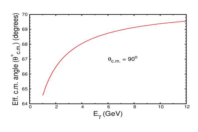
Figure 3: Effective center of mass angle vs the incident photon energy.

It follows from the above equation, for large momentum transfer, that, therefore for the same $s$, the $pd\rightarrow pd$ scattering will take place at smaller angles in the $pd$ center-of-mass reference frame. To evaluate this difference we introduce $\theta_{cm}^{*}$ which represents the center-of-mass scattering angle for the $pd\rightarrow pd$ reaction in the form

$$t_{pd}=(p_{df}-p_{di})^{2}=2(m_{d}^{2}-E_{d,cm}^{2})(1-\cos\theta_{cm}^{*}),$$ (34)

where $E_{d,cm}=\frac{s+m_{d}^{2}-m_{N}^{2}}{2\sqrt{s}}$. Then, comparing this equation with Eq. (5) in the asymptotic limit of high energies, one finds that for $\theta_{cm}=90^{o}$ in reaction (2) the asymptotic limit of the effective center-of-mass scattering angle of $pd\rightarrow pd$ scattering is $\theta_{cm}^{*}=70.53^{o}$. The dependence of $\theta_{cm}^{*}$ at finite energies on the incoming photon is shown in Fig. 3. The figure indicates that, for realistic comparison of HRM prediction with the data, one needs the $pd\rightarrow pd$ cross section for the range of center-of-mass scattering angles.

To achieve this, we parametrized the existing experimental data on elastic $pd\rightarrow pd$ scattering 1.0GeV ; 582MeV ; 641.3MeV ; 800MeV ; 4.50GeV which covers the invariant energy range of $s\sim$ 9.5 - 17.3 GeV². The following parametric form is used to fit the $pd\rightarrow pd$ cross section data:

$$\frac{d\sigma_{pd}}{dt}(s,\cos\theta_{cm}^{*})=\frac{1}{(s/10)^{16}}\frac{A(s)e^{B(\cos\theta_{cm}^{*})}}{(1-\cos^{2}\theta_{cm}^{*})^{3}},$$ (35)

where $A(s)=Ce^{(a_{1}s+a_{2}s^{2})}$ and $B(x)=bx+cx^{2}$, with the fit parameters given in Table 1. The samples of fits obtained for the elastic $pd\rightarrow pd$ hard scattering are presented in Fig. 4.

$C$ ($\mu$b GeV30)	$a_{1}$ (GeV-2)	$a_{2}$ (GeV-4)	b	c
(9.72 $\pm$ 1.33) $\times$ 104	-0.98 $\pm$ 0.05	0.04 $\pm$ 0.001	3.45 $\pm$ 0.02	-0.83 $\pm$ 0.05

Table 1: Fit Parameters.

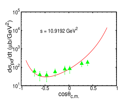
(a)

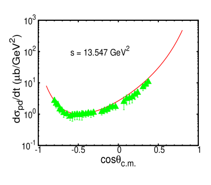
(b)

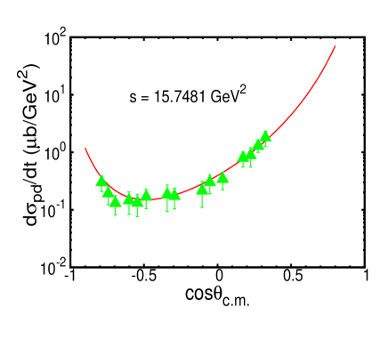
(c)

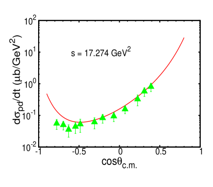
(d)

Figure 4: Fits of elastic $pd\rightarrow pd$ scattering cross section. The data in (a) are from 800MeV and in (b),(c) and (d) are from 4.50GeV . The curves are the fits to the data obtained using Eq. (35) with fit parameters from Table (1).

The errors quoted in the table for the fitting parameters result in a overall error in the $pd\to pd$ cross section on the level of 22-37%. Note that the form of the ansatz used in Eq. (35) is in agreement with the energy and angular dependence following from the quark interchange mechanism of the $pd$ elastic scattering. As a result the ansatz is strictly valid for large center-of-mass angles $|cos(\theta_{cm}^{*})|\leq 0.6$. However we extended the fitting procedure beyond this angular range by introducing an additional function $e^{B(\cos\theta_{cm}^{*})}$.

IV.1.3 Estimation of the effective charge $Q_{eff}$.

To calculate the effective quark charge associated with the hard rescattering amplitude, we notice that from Eq. (15) it follows that $Q_{eff}$ should satisfy the following relation:

$$\sum\limits_{i\in p}Q_{i}\langle d^{\prime}p^{\prime}\mid M_{pd,i}\mid dp\rangle=Q_{eff}\langle d^{\prime}p^{\prime}|M_{pd}\mid dp\rangle,$$ (36)

where by $i$ we sum by the quarks in the proton that were struck by incoming photon. To use the above equation one needs a specific model for $pd$ elastic scattering which explicitly uses underlying quark degrees of the freedom in $pd$ scattering. For such a model we use the quark-interchange mechanism (QIM). The consideration of a quark-interchange mechanism is justified if one works in the regime in which the $pd$ elastic scattering exhibits scaling in agreement with quark counting rule, i.e., $s^{-16}$.

Similar to Refs.gdpn ; gheppn ; gdBB , within the QIM $Q_{eff}$ can be estimated using the relation

$$Q_{eff}=\frac{N_{uu}(Q_{u})+N_{dd}(Q_{d})+N_{ud}(Q_{u}+Q_{d})}{N_{uu}+N_{dd}+N_{ud}},$$ (37)

where $Q_{i}$ is the charge of the $u$ and $d$ valence quarks in the proton $p$ and $N_{ii}$ represents the number of quark interchanges for $u$ and $d$ flavors necessary to produce a given helicity $pd$ amplitude. Note that for the particular case of elastic $pd$ scattering $N_{ud}=0$, and one obtains $Q_{eff}=\frac{1}{3}$.

IV.1.4 Final expression for the differential cross section

Substituting Eq. (31) into Eq. (25) and taking into account the above estimation of $Q_{eff}$, we arrive at the final expression for the differential cross section which will be used for the numerical estimates:

$$\frac{d\sigma}{dt}(s,t)=\frac{2\pi^{4}\alpha}{3s^{\prime}_{{}^{3}\text{He}}}\Big{(}\frac{s^{\prime}_{N}}{s^{\prime}_{{}^{3}\text{He}}}\Big{)}\frac{d\sigma_{pd}}{dt}(s,t_{pd})\cdot m_{N}S^{NR}_{{}^{3}\text{He}/d}(p_{1z}=0),$$ (38)

where $\alpha=\frac{e^{2}}{4\pi}$ is the fine structure constant. For the evaluation of the transition spectral function $S^{NR}_{{}^{3}\text{He}/d}$, we use the realistic ${}^{3}\text{He}$ Nogga:2002 and deuteron Wiringa:1994wb wave functions based on the V18 potentialWiringa:1994wb of $NN$ interaction. This yieldseheppnII $S^{NR}_{{}^{3}\text{He}/d}(p_{1z}=0)=4.1\times 10^{-4}$ GeV. For the differential cross section of the large center-of-mass elastic $pd\rightarrow pd$ scattering, $\frac{d\sigma_{pd}}{dt}(s,t_{pd})$, we use Eq. (35) which covers the invariant energy range of up to $s=17.3$ GeV², corresponding to $E_{\gamma}=1.67$ GeV for the reaction (2). In Fig. 5 we present the comparison of our calculation of the energy dependence of the $s^{17}$ scaled differential cross section at $\theta_{cm}=90^{0}$ with the data of Ref.Pomerantz13 . The shaded area represents the error due to the above discussed fitting of the elastic $pd\rightarrow pd$ cross sections.

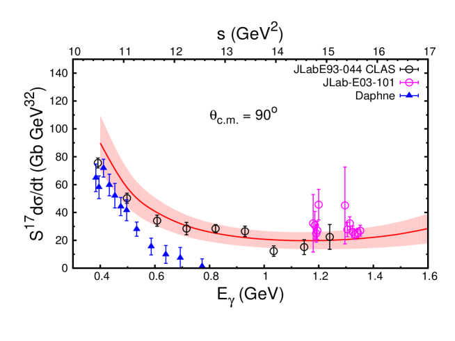
Figure 5: Energy dependence of the differential cross section at $\theta_{cm}=90^{0}$ scaled by an $s^{17}$ factor. The solid curve is the calculation according to Eq. (38). The experimental data are from Refs.DAPHNE ; Pomerantz13 ; Berman . See also the discussion in Ref.Pomerantz13 on disagreement between DAPHNE and JLAB/CLAS data.

As the comparison shows, Eq. (38) describes surprisingly well the Jefferson Lab data, considering the fact that the cross section between $E_{\gamma}=0.4$ GeV and $E_{\gamma}=1.3$ GeV drops by a factor of $\sim 4000$. It is interesting that the HRM model describes data reasonably well even for the range of $E_{\gamma}<1$ GeV for which the general conditions for the onset of QCD degrees of freedom is not satisfied (see the discussion in Sec. II). This situation is specific to the HRM model in which there is another scale $t_{pd}$, the invariant momentum transfer in the hard rescattering amplitude. The $-t_{pd}>1$ GeV² condition is necessary for the factorization of the hard scattering kernels from the soft nuclear parts. It follows from Eq. (33) that such a threshold for $t_{pd}$ is reached already for incoming photon energies of 0.7 GeV. Considering the photon energies below 0.7 GeV, the qualitative agreement of the HRM model with the data is an indication of the smooth transition from the hard to the soft regime of the interaction.

The HRM model allows us to also calculate the angular distribution of the differential cross section for fixed values of $s$. In Fig. 6 we present predictions for angular distribution of the energy scaled differential cross section at largest photon energies for which there are available dataYI .

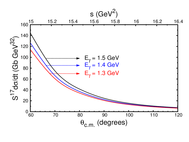
Figure 6: The angular dependence of $s^{17}$ scaled differential cross section for incoming photon energies of 1.3, 1.4, and 1.5 GeV.

The interesting feature of the HRM prediction is that, due to the fact that the magnitude of invariant momentum transfer of the reaction (2), $t$, is larger than that of the $pd\rightarrow pd$ scattering, $t_{pd}$ [Eq. (33)], the effective center-of-mass angle in the latter case, $\theta^{*}_{cm}<\theta_{cm}$ (see Fig. 3); as a result HRM predicts angular distributions that are monotonically decreasing with an increase of $\theta_{cm}$ for up to $\theta_{cm}\approx 120^{0}$.

Finally in Fig. 7 we present the calculation of the $s^{17}$ scaled differential cross section as a function of incoming photon energy for different fixed and large center-of-mass angles, $\theta_{cm}$. Note that in both Figs. 6 and 7 the accuracy of the theoretical predictions is similar to that of the energy dependence at $\theta_{cm}=90^{0}$ presented in Fig. 5.

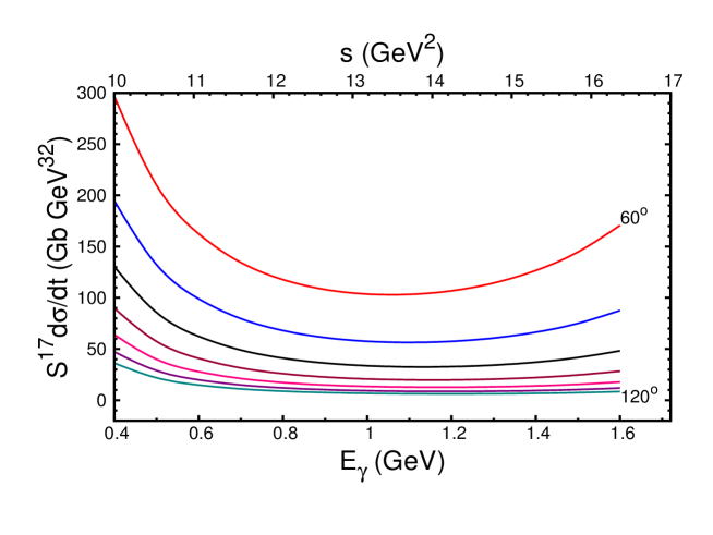
Figure 7: Energy dependence of the $s^{17}$ scaled differential cross section for different values of $\theta_{cm}$. The upper curve corresponds to $\theta_{cm}=60^{o}$, with the following curves corresponding to increment of the center-of-mass angle by $10^{o}$.

The possibility of comparing these calculations with the experimental data will allow us to ascertain the range of validity of the HRM mechanism. These comparisons will allow us to identify the minimal momentum transfer in these nuclear reactions for which one observes the onset of QCD degrees of freedom.

V Summary and Outlook

We extended the consideration of the hard rescattering mechanism of two-body breakup reactions to the high energy photodisintegration of the ${}^{3}\text{He}$ target to the ($p,d$) pair at large center-of-mass angles. The obtained expression for the cross section does not contain free parameters and is expressed through the effective charge of the constituent quarks being struck by the incoming photon and interchanged in the final state of the process, the ${}^{3}\text{He}\rightarrow pd$ transition spectral function, and the hard elastic $pd\rightarrow pd$ scattering differential cross section.

For numerical results we estimated the effective quark charge based on the quark-interchange model of $pd\rightarrow pd$ scattering. The transition spectral function is calculated using realistic wave functions of ${}^{3}\text{He}$ and the deuteron and the $pd\rightarrow pd$ cross section is taken from the experiment. The calculated differential cross section of reaction (2) at $\theta_{cm}=90^{0}$ is compared with the recent experimental data from Jefferson Lab. The comparison shows a rather good agreement with the data for the range of photon energies $E_{\gamma}\gtrsim 0.7$ GeV. We also give predictions for angular distribution of the cross section, which reflects the special property of HRM in which the magnitude of the invariant momentum transfer entering in the reaction (2) exceeds the one entering in the hard amplitude of $pd\rightarrow pd$ scattering. The possibility of comparing the energy dependence of the cross section for different $\theta_{cm}$ of the $pd$ breakup will allow us to establish the kinematic boundaries in which QCD degrees of freedom are important for the quantitative description of the hard $pd$ breakup reactions.

Acknowledgements: We are thankful to Drs. Y. Ilieava, E. Piasetzky, and I. Pomerantz for numerous discussions and comments as well as explanation of the experimental data. This work is supported by a U.S. DOE grant under Contract No. DE-FG02-01ER41172.

Appendix A

A.1 Nuclear and Nucleonic wave functions

In this appendix, the details on derivation of the wave functions of the ${}^{3}\text{He}$ nucleus and deuteron are discussed. We begin with considering the part ${\bf A}$ in Eq. (III) related to the ${}^{3}\text{He}\rightarrow d$ nuclear transition

$$A_{1}=\int(-i)\frac{\chi_{d}^{*^{\lambda_{d}}}\Gamma_{{}_{DNN}}^{\dagger}}{p_{d}^{2}-m_{{}_{d}}^{2}+i\epsilon}\frac{i(\not{p}_{3}+m)}{p_{3}^{2}-m_{N}^{2}+i\epsilon}\frac{i(\not{p}_{2}+m)}{p_{2}^{2}-m_{N}^{2}+i\epsilon}\frac{i(\not{p}_{1}+m)}{p_{1}^{2}-m_{N}^{2}+i\epsilon}$$

$$\times\qquad i\Gamma_{{}_{{}^{3}\text{He}}}\chi_{{}_{{}^{3}\text{He}}}^{\lambda_{{}^{3}\text{He}}}\frac{1}{2}\frac{dp_{{}_{2+}}dp_{{}_{2-}}d^{2}p_{{}_{2\perp}}}{(2\pi)^{4}}\frac{1}{2}\frac{dp_{{}_{3+}}dp_{{}_{3-}}d^{2}p_{{}_{3\perp}}}{(2\pi)^{4}},$$ (A-1)

where the $d^{4}p$ differentials are expressed in terms of the light cone momenta. The denominators of the propagators in this expression can be expanded as follows:

$$p^{2}-m_{N}^{2}+i\epsilon=p_{{}_{+}}\Big{(}p_{{}_{-}}-\frac{m_{N}^{2}+p_{{}_{\perp}}^{2}}{p_{+}}+i\epsilon^{\prime}\Big{)},$$ (A-2)

in which using the relations $p_{1-}=p_{{}^{3}\text{He}-}-p_{d-}$ and $p_{d-}=\frac{m_{d}^{2}+p_{d\perp}^{2}}{p_{d+}}$ one obtains

$$p_{1}^{2}-m_{N}^{2}+i\epsilon=\frac{1}{p_{{}_{{}^{3}\text{He}+}}}\Big{(}m_{{}_{{}^{3}\text{He}}}^{2}-\frac{m_{{}_{d}}^{2}+p_{{}_{d\perp}}^{2}}{\beta_{d}}-\frac{m_{N}^{2}+p_{{}_{1\perp}}^{2}}{\beta_{1}}\Big{)},$$ (A-3)

where $\beta_{1}=\frac{p_{{}_{1+}}}{p_{{}_{{}^{3}\text{He}+}}}$, $\beta_{d}=\frac{p_{{}_{d+}}}{p_{{}_{{}^{3}\text{He}+}}}$ and $\beta_{1}+\beta_{d}=1$. Using the sum rule relation, $(\not{p}+m)=\sum_{\lambda}u(p,\lambda)\bar{u}(p,\lambda)$, one introduces the light-front wave function of ${}^{3}\text{He}$ (see, e.g., FS81 ; pAjj ; multisrc ) as follows:

$$\Psi_{{}_{{}^{3}\text{He}}}^{{}^{\lambda_{{}^{3}\text{He}}}}(\beta_{1},\lambda_{1},p_{{}_{1\perp}},\beta_{2},p_{{}_{2\perp}}\lambda_{2},\lambda_{3})=\frac{\bar{u}(p_{3},\lambda_{3})\bar{u}(p_{2},\lambda_{2})\bar{u}(p_{1},\lambda_{1})}{\Big{(}m_{{}_{{}^{3}\text{He}}}^{2}-\frac{m_{{}_{d}}^{2}+p_{d\perp}^{2}}{\beta_{d}}-\frac{m_{N}^{2}+p_{{1\perp}}^{2}}{\beta_{1}}\Big{)}}\Gamma_{{}_{{}^{3}\text{He}}}\chi_{{}_{{}^{3}\text{He}}}^{\lambda_{{}^{3}\text{He}}}.$$ (A-4)

This wave function gives the probability amplitude of finding the ${}^{3}\text{He}$ nucleus with helicity $\lambda_{{}^{3}\text{He}}$ consisting of nucleons with momenta $p_{i}$ and helicities $\lambda_{i}$, $i=1,2,3$. Using the above definition of the ${}^{3}\text{He}$ wave function and Eq. (A-3) in Eq. (A.1), one obtains

$$A_{1}=-i\sum_{\lambda_{d},\lambda_{3},\lambda_{2},\lambda_{1}}\int\frac{\chi_{d}^{*^{\lambda_{d}}}\Gamma_{{}_{DNN}}^{\dagger}}{p_{d}^{2}-m_{{}_{d}}^{2}+i\epsilon}u(p_{3},\lambda_{3})u(p_{2},\lambda_{2})u(p_{1},\lambda_{1})\frac{1}{p_{{}_{2+}}\Big{(}p_{{}_{2-}}-\frac{m_{N}^{2}+p_{{}_{2\perp}}^{2}}{p_{{}_{2+}}}\Big{)}}$$

$$\times\frac{\Psi_{{}_{{}^{3}\text{He}}}^{{}^{\lambda_{{}^{3}\text{He}}}}(\beta_{1},\lambda_{1},p_{{}_{1\perp}},\beta_{2},p_{{}_{2\perp}}\lambda_{2},\lambda_{3})}{\beta_{1}}\frac{1}{2}\frac{dp_{{}_{2-}}dp_{{}_{2+}}d^{2}p_{{}_{2\perp}}}{(2\pi)^{4}}\frac{1}{2}\frac{d\beta_{3}}{\beta_{3}}\frac{d^{2}p_{{}_{3\perp}}}{(2\pi)^{3}},$$ (A-5)

where $\beta_{3}=\frac{p_{3+}}{p_{{}^{3}\text{He}+}}$ and the integral over $p_{3-}$ is performed at its pole value:

$$\int\frac{dp_{-}}{p_{-}-\frac{m_{N}^{2}+p_{\perp}^{2}}{p_{+}}+i\epsilon}=-2\pi i|_{p_{-}=\frac{m_{N}^{2}+p_{\perp}^{2}}{p_{+}}}.$$ (A-6)

Since $p_{2}+p_{3}=p_{d}$, the differentials with respect to $p_{2}$ can be written as

$$\frac{dp_{{}_{2-}}dp_{{}_{2+}}dp_{{}_{2\perp}}}{(2\pi)^{4}}=\frac{dp_{{}_{d-}}dp_{{}_{d+}}dp_{{}_{d\perp}}}{(2\pi)^{4}}.$$ (A-7)

Also, the quantity $p_{{}_{2+}}\big{(}p_{{}_{2-}}-\frac{m_{N}^{2}+p_{{}_{2\perp}}^{2}}{p_{{}_{2+}}}\big{)}$ in Eq. (A.1) can be represented as:

$$p_{{}_{2+}}\Big{(}p_{{}_{2-}}-\frac{p_{{}_{2\perp}}^{2}+m_{N}^{2}}{p_{{}_{2+}}}\Big{)}=(1-\alpha_{3})\Big{(}m_{{}_{d}}^{2}+p_{{}_{d\perp}}^{2}-\frac{m_{N}^{2}+p_{{}_{3\perp}}^{2}}{\alpha_{3}}-\frac{m_{N}^{2}+p_{{}_{2\perp}}^{2}}{1-\alpha_{3}}\Big{)},$$ (A-8)

where we define $\alpha_{3}=\frac{p_{{}_{3+}}}{p_{{}_{d+}}}\equiv\frac{\beta_{3}}{\beta_{d}}$ and $1-\alpha_{3}\equiv\alpha_{2}=\frac{p_{{}_{2+}}}{p_{{}_{d+}}}=\frac{\beta_{2}}{\beta_{d}}\text{ with }\beta_{d}=\frac{p_{d+}}{p_{{}^{3}\text{He}+}}\text{ and }\beta_{2}=\frac{p_{2+}}{p_{{}^{3}\text{He}+}}$. The quantities $\alpha_{3}$ and $\alpha_{2}$ represent the fractions of the momentum of the intermediate deuteron carried by the nucleons 3 and 2 respectively. Note that $\alpha_{3}+\alpha_{2}=1$.

Similar to Eq. (A-4), we introduce light-front wave function of the deuteronFS81 ; pAjj ; multisrc :

$$\Psi_{{}_{d}}^{\lambda_{d}}(\alpha_{3},p_{{}_{3\perp}},p_{{}_{d\perp}})=\frac{\bar{u}(p_{2},\lambda_{2})\bar{u}(p_{3},\lambda_{3})}{\Big{(}m_{{}_{d}}^{2}+p_{{}_{d\perp}}^{2}-\frac{m_{N}^{2}+p_{{}_{3\perp}}^{2}}{\alpha_{3}}-\frac{m_{N}^{2}+p_{{}_{2\perp}}^{2}}{1-\alpha_{3}}\Big{)}}\Gamma_{{}_{DNN}}\chi_{{}_{d}}^{{}^{\lambda_{d}}},$$ (A-9)

which describes the probability amplitude of finding in the $\lambda_{d}$-helicity deuteron two nucleons with momenta $p_{i}$ and helicities $\lambda_{i}$, $i=1,2$. Using Eqs.(A-8) and (A-9) for Eq. (A.1) we obtain

$$A_{1}= -i\sum_{\lambda_{d},\lambda_{3},\lambda_{2},\lambda_{1}}\int\frac{\Psi_{{}_{d}}^{\dagger\lambda_{d}:\lambda_{2},\lambda_{3}}(\alpha_{3},p_{{}_{3\perp}},p_{{}_{d\perp}})}{1-\alpha_{3}}u(p_{1},\lambda_{1})\frac{\Psi_{{}_{{}^{3}\text{He}}}^{{}^{\lambda_{{}^{3}\text{He}}}}(\beta_{1},\lambda_{1},p_{{}_{1\perp}},\beta_{2},p_{{}_{2\perp}}\lambda_{2},\lambda_{3})}{\beta_{1}}$$ (A-10)

$$\times\frac{1}{2}\frac{d\beta_{{}_{d}}d^{2}p_{{}_{d\perp}}}{\beta_{d}(2\pi)^{3}}\frac{1}{2}\frac{d\beta_{3}}{\beta_{3}}\frac{d^{2}p_{{}_{3\perp}}}{(2\pi)^{3}},$$

where the $p_{2-}$ integration is performed similar to that of $p_{3-}$ according to Eq. (A-6).

Next, we consider the second part of the expression $A$ in Eq. (III) related to the transition of the deuteron from intermediate to the final state:

$$A_{2} =-\int\chi_{d}^{*\lambda_{d}}(\Gamma_{{}_{DNN}}^{\dagger})\frac{i(\not{p}_{2f}+m)}{p_{2f}^{2}-m_{N}^{2}+i\epsilon}\frac{i(\not{p}_{3}^{\prime}+m)}{p_{3}^{\prime 2}-m_{N}^{2}+i\epsilon}\frac{i(\not{p}_{2}^{\prime}+m)}{p_{2}^{\prime 2}-m_{N}^{2}+i\epsilon}i\Gamma_{{}_{DNN}}\chi_{d}^{\lambda_{d}}\frac{d^{4}p_{3}^{\prime}}{(2\pi)^{4}}$$ (A-11)

$$=-\sum_{\begin{subarray}{c}\lambda_{2f}\\ \lambda_{2}^{\prime},\lambda_{3}^{\prime}\end{subarray}}\int\chi_{d}^{*\lambda_{d}}\Gamma_{{}_{DNN}}^{\dagger}\frac{u(p_{2f},\lambda_{2f})\bar{u}(p_{2f},\lambda_{2f})}{p_{2f}^{2}-m_{N}^{2}+i\epsilon}\frac{u(p_{2}^{\prime},\lambda_{2}^{\prime})\bar{u}(p_{2}^{\prime},\lambda_{2}^{\prime})}{p_{{}_{2+}}^{\prime}\Big{(}p_{{}_{2-}}^{\prime}-\frac{m_{N}^{2}+p_{2\perp}^{\prime 2}}{p_{{}_{2+}}^{\prime}}+i\epsilon\Big{)}}$$

$$\times\qquad u(p_{3}^{\prime},\lambda_{3}^{\prime})\bar{u}(p_{3}^{\prime},\lambda_{3}^{\prime})i\Gamma_{{}_{DNN}}\chi_{d}^{\lambda_{d}}\frac{1}{2}\frac{dp_{{}_{3+}}^{\prime}}{p_{{}_{3+}}^{\prime}}\frac{d^{2}p_{{}_{3\perp}}^{\prime}}{(2\pi)^{3}},$$

where the $dp_{3-}^{\prime}$ is integrated according to Eq. (A-6). To estimate the denominator $p_{2f}^{2}-m_{N}^{2}+i\epsilon$ we use the relation $p_{2f}=p_{df}-p_{3}^{\prime}$, which allows us to express

$$p_{2f}^{2}-m_{N}^{2}+i\epsilon=\frac{p_{{}_{2f+}}}{p_{{}_{df+}}}\Big{(}m_{d}^{2}+p_{{}_{df\perp}}^{2}-\frac{m_{N}^{2}+p_{{}_{3\perp}}^{\prime 2}}{p_{{}_{3+}}^{\prime}/p_{{}_{df+}}}-\frac{m_{N}^{2}+p_{{}_{2f\perp}}^{2}}{p_{{}_{2f+}}/p_{{}_{df+}}}+i\epsilon\Big{)}.$$ (A-12)

Defining $\frac{p_{{}_{3+}}^{\prime}}{p_{{}_{df+}}}=\frac{p_{{}_{3+}}^{\prime}/p_{{}_{d+}}}{p_{{}_{df+}}/p_{{}_{d+}}}=\frac{\alpha_{3}^{\prime}}{\gamma_{d}}$ and $\frac{p_{{}_{2f+}}}{p_{{}_{df+}}}=1-\frac{p_{{}_{3+}}^{\prime}}{p_{{}_{df+}}}=1-\frac{\alpha_{3}^{\prime}}{\gamma_{d}}$, the above equation reduces to:

$$p_{2f}^{2}-m_{N}^{2}+i\epsilon=(1-\frac{\alpha_{3}^{\prime}}{\gamma_{d}})\Big{(}m_{d}^{2}+p_{{}_{df\perp}}^{2}-\frac{m_{N}^{2}+p_{{}_{3\perp}}^{\prime 2}}{\alpha_{3}^{\prime}/\gamma_{d}}-\frac{m_{N}^{2}+p_{{}_{2f\perp}}^{2}}{1-\alpha_{3}^{\prime}/\gamma_{d}}+i\epsilon\Big{)},$$ (A-13)

where the quantity $\gamma_{d}=\frac{p_{{}_{df+}}}{p_{{}_{d+}}}$ is the fraction of the momentum of the intermediate deuteron carried by the final deuteron. Using Eqs.(A-9) and (A-13), we rewrite Eq. (A-11) as follows:

$$A_{2} =\sum_{\begin{subarray}{c}\lambda_{df},\lambda_{2f}\\ \lambda_{2}^{\prime},\lambda_{3}^{\prime}\end{subarray}}\int\frac{{\Psi_{d}^{\dagger\lambda_{df}:\lambda_{3}^{\prime},\lambda_{2f}}}(\alpha_{2f}/\gamma_{d},p_{2\perp},\alpha_{3}^{\prime}/\gamma_{d},p_{3\perp}^{\prime})}{1-\alpha_{3}^{\prime}/\gamma_{d}}\bar{u}(p_{2f},\lambda_{2f})u(p_{2}^{\prime},\lambda_{2}^{\prime})$$ (A-14)

$$\times\qquad\frac{\Psi_{d}^{\lambda_{d}:\lambda_{2}^{\prime},\lambda_{3}^{\prime}}(\alpha_{3}^{\prime},p_{d\perp},p_{3\perp}^{\prime})}{1-\alpha_{3}^{\prime}}\frac{1}{2}\frac{d\alpha_{3}^{\prime}}{\alpha_{3}^{\prime}}\frac{d^{2}p_{3\perp}^{\prime}}{(2\pi)^{3}}.$$

Now we consider the $N1$ part of the amplitude in Eq. (III), which describes the transition of the nucleon with momentum $p_{1}$ to the final nucleon with momentum $p_{1f}$. Using on-shell sum-rule relations for the numerators of the quark propagators for the $N1$ part, one has

$$N1=\sum_{\begin{subarray}{c}\lambda_{1}\\ \eta_{1f},\eta_{1}\end{subarray}}\int\bar{u}(p_{1f},\lambda_{1f})(-i)\Gamma_{n1f}^{\dagger}\frac{u_{q}(p_{1f}-k_{1},\eta_{1f})\bar{u}_{q}(p_{1f}-k_{1},\eta_{1f})}{(p_{1f}-k_{1})^{2}-m_{q}^{2}+i\epsilon}\Big{[}-igT_{c}^{\beta}\gamma_{\mu}\Big{]}$$

$$\times\frac{\Psi_{s}(k_{1})\bar{\Psi}_{s}(k_{1})}{k_{1}^{2}-m_{s}^{2}+i\epsilon}\frac{u_{q}(p_{1}-k_{1},\eta_{1})\bar{u}_{q}(p_{1}-k_{1},\eta_{1})}{(p_{1}-k_{1})^{2}-m_{q}^{2}+i\epsilon}i\Gamma_{n1}u(p_{1},\lambda_{1})\frac{1}{2}\dfrac{dk_{1+}dk_{1-}d^{2}k_{1\perp}}{(2\pi)^{4}},$$ (A-15)

where we sum over the initial helicity ($\eta_{1}$) of the quark before being struck by the incoming photon and the final helicity ($\eta_{1f}$) of the quark that recombines to form the final state proton. In Eq. (A.1), we can expand the denominators of the propagators as follows:

$$(p_{1f}-k_{1})^{2}-m_{q}^{2}+i\epsilon=(1-x_{s1})\Big{(}m_{N}^{2}+p_{1f\perp}^{2}-\frac{m_{s}^{2}+k_{1\perp}^{2}}{x_{s1}}-\frac{m_{q}^{2}+(p_{1f}-k_{1})_{\perp}^{2}}{1-x_{s1}}+i\epsilon\Big{)}$$

$$(p_{1}-k_{1})^{2}-m_{q}^{2}+i\epsilon=(1-x_{1})\Big{(}m_{N}^{2}+p_{1\perp}^{2}-\frac{m_{s}^{2}+k_{1\perp}^{2}}{x_{1}}-\frac{m_{q}^{2}+(p_{1}-k_{1})_{\perp}^{2}}{1-x_{1}}+i\epsilon\Big{)},$$

where $x_{s1}=\frac{k_{1+}}{p_{1f+}}\text{ and }x_{1}=\frac{k_{1+}}{p_{1+}}$ along with $k_{1-}=\frac{m_{s}^{2}+k_{1\perp}^{2}}{k_{1+}}$ and $p_{1f-}=\frac{m_{N}^{2}+p_{1f\perp}^{2}}{p_{1f+}}$. Here $x_{1}(x_{s1})$ is interpreted as the momentum fraction of the initial (final) nucleon “1” carried by the spectator quark system. Performing the $dk_{1-}$ integration at the $k_{1-}$ pole value of the spectator system allows us to introduce a single quark wave function of the nucleon in the form

$$\Psi_{n}^{\lambda;\eta}(X,k_{\perp},p_{\perp})=\frac{\bar{u}_{q}(p-k,\eta)\bar{\Psi}_{s}(k)}{m_{N}^{2}+p_{\perp}^{2}-\frac{m_{s}^{2}+k_{\perp}^{2}}{X}-\frac{m_{q}^{2}+(p-k)_{\perp}^{2}}{1-X}}\Gamma_{n}u(p,\lambda),$$ (A-17)

which describes the probability amplitude of finding a quark with helicity $\eta$ and momentum fraction $1-x$ in the $\lambda$-helicity nucleon with momentum $p$. With this definition of quark wave function of the nucleon one obtains for the $N1$ part

$$N1 =i\sum_{\begin{subarray}{c}\lambda_{1}\\ \eta_{1f},\eta_{1}\end{subarray}}\int\frac{\Psi_{n1f}^{\dagger\lambda_{1f};\eta_{1f}}(x_{s1},k_{1\perp},p_{1f\perp})}{1-x_{s1}}\bar{u}_{q}(p_{1f}-k_{1},\eta_{1f})u_{q}(p_{1}-k_{1},\eta_{1})$$ (A-18)

$$\times\Big{[}-igT_{c}^{\beta}\gamma_{\mu}\Big{]}\frac{\Psi_{n1}^{\lambda_{1};\eta_{1}}(x_{1},k_{1\perp},p_{1\perp})}{1-x_{1}}\frac{1}{2}\dfrac{dx_{1}}{x_{1}}\dfrac{d^{2}k_{1\perp}}{(2\pi)^{3}}.$$

Performing very similar calculations for the $N2$ part of Eq. (III), one obtains:

$$N2 =-\sum_{\begin{subarray}{c}\lambda_{2f},\lambda_{2}^{\prime}\\ \eta_{2f},\eta_{2}^{\prime}\end{subarray}}\int\frac{\Psi_{n2f}^{\dagger\lambda_{2f};\eta_{2f}}(x_{s2},k_{2\perp},p_{2f\perp})}{1-x_{s2}}\bar{u}_{q}(p_{2f}-k_{2},\eta_{2f})u_{q}(p_{2}^{\prime}-k_{2},\eta_{2}^{\prime})$$ (A-19)

$$\times\frac{\Psi_{n2^{\prime}}^{\lambda_{2}^{\prime};\eta_{2}^{\prime}}(x_{2}^{\prime},k_{2\perp},p_{2\perp}^{\prime})}{1-x_{2}^{\prime}}\frac{1}{2}\dfrac{dx_{2}^{\prime}}{x_{2}^{\prime}}\dfrac{d^{2}k_{2\perp}}{(2\pi)^{3}},$$

where $x_{s2}=\frac{k_{2+}}{p_{2f+}}$ and $x_{2}^{\prime}=\frac{k_{2+}}{p_{2+}^{\prime}}$.

Substituting now Eqs. (A-10), (A-14), (A-18), and (A-19) into Eq. (III), one obtains

$$\mathcal{M}^{\lambda_{df},\lambda_{1f};\lambda_{{}^{3}\text{He}},h}=\sum_{\begin{subarray}{c}(\lambda_{2f})(\lambda_{2}^{\prime},\lambda_{3}^{\prime})(\lambda_{d})\\ (\lambda_{1},\lambda_{2},\lambda_{3})\\ (\eta_{1f},\eta_{2f})(\eta_{1},\eta_{2}^{\prime})\end{subarray}}\int\frac{{\Psi_{d}^{\dagger\lambda_{df}:\lambda_{3}^{\prime},\lambda_{2f}}}(\alpha_{2f}/\gamma_{d},p_{2\perp},\alpha_{3}^{\prime}/\gamma_{d},p_{3\perp}^{\prime})}{1-\alpha_{3}^{\prime}/\gamma_{d}}\Bigg{\{}\frac{\Psi_{n2f}^{\dagger\lambda_{2f};\eta_{2f}}(x_{s2},k_{2\perp},p_{2f\perp})}{1-x_{s2}}$$

$$\times\bar{u}_{q}(p_{2f}-k_{2},\eta_{2f})[-igT_{c}^{\alpha}\gamma_{\nu}]\Big{[}\frac{i(\not{p}_{1}+\not{q}-\not{p_{1}}+m_{q})}{(p_{1}-k_{1}+q)^{2}-m_{q}^{2}+i\epsilon}\Big{]}[-ie\epsilon^{\mu}\gamma\mu]u_{q}(p_{1}-k_{1},\eta_{1})$$

$$\times\frac{\Psi_{n1}^{\lambda_{1};\eta_{1}}(x_{1},k_{1\perp},p_{1\perp})}{1-x_{1}}\Bigg{\}}_{1}\Bigg{\{}\frac{\Psi_{n1f}^{\dagger\lambda_{1f};\eta_{1f}}(x_{s1},k_{1\perp},p_{1f\perp})}{1-x_{s1}}\bar{u}_{q}(p_{1f}-k_{1},\eta_{1f})[-igT_{c}^{\beta}\gamma_{\mu}]u_{q}(p_{2}^{\prime}-k_{2},\eta_{2}^{\prime})$$

$$\times\frac{\Psi_{n2^{\prime}}^{\lambda_{2}^{\prime};\eta_{2}^{\prime}}(x_{2}^{\prime},k_{2\perp},p_{2\perp}^{\prime})}{1-x_{2}^{\prime}}\Bigg{\}}_{2}G^{\mu\nu}(r)\frac{\Psi_{d}^{\lambda_{d}:\lambda_{2}^{\prime},\lambda_{3}^{\prime}}(\alpha_{3}^{\prime},p_{d\perp},p_{3\perp}^{\prime})}{1-\alpha_{3}^{\prime}}\frac{\Psi_{{}_{d}}^{\dagger\lambda_{d}:\lambda_{2},\lambda_{3}}(\alpha_{3},p_{{}_{3\perp}},p_{{}_{d\perp}})}{(1-\alpha_{3})}$$

$$\times\frac{\Psi_{{}_{{}^{3}\text{He}}}^{{}^{\lambda_{{}^{3}\text{He}}}}(\beta_{1},\lambda_{1},p_{{}_{1\perp}},\beta_{2},p_{{}_{2\perp}}\lambda_{2},\lambda_{3})}{\beta_{1}}\frac{d\beta_{d}}{\beta_{d}}\frac{d^{2}p_{d\perp}}{2(2\pi)^{3}}\frac{d\beta_{3}}{\beta_{3}}\frac{d^{2}p_{3\perp}}{2(2\pi)^{3}}\frac{d\alpha_{3}^{\prime}}{\alpha_{3}^{\prime}}\frac{d^{2}p_{3\perp}^{\prime}}{2(2\pi)^{3}}\frac{dx_{1}}{x_{1}}\frac{d^{2}k_{1\perp}}{2(2\pi)^{3}}\frac{dx_{2}^{\prime}}{x_{2}^{\prime}}\frac{d^{2}k_{2\perp}}{2(2\pi)^{3}}.$$ (A-20)

A.2 Hard scattering kernel

In Eq. (A.1), the expression in $\{\}_{1}\{\}_{2}G^{\mu\nu}(r)$ describes the hard photon-quark interaction followed by a quark interchange through the gluon exchange.

A.2.1 Propagator of the struck quark

We analyze first the propagator of the struck quark, $\frac{i(\not{p}_{1}+\not{q}-\not{k_{1}}+m_{q})}{(p_{1}-k_{1}+q)^{2}-m_{q}^{2}+i\epsilon}$.

Using the definition of the reference frame from Eq. (6) and momentum fraction definitions $\beta_{1}=\frac{p_{1+}}{p_{{}^{3}\text{He}+}}=\frac{p_{1+}}{\sqrt{s^{\prime}_{{}^{3}\text{He}}}}$ and $x_{1}=\frac{k_{1+}}{p_{1+}}$, one can isolate the pole term in the denominator of the struck quark propagator as follows:

$$(p_{1}-k_{1}+q)^{2}-m_{q}^{2}+i\epsilon=(p_{1+}-p_{1+}x_{1})(p_{1-}-k_{1-}+q_{-})-(p_{1\perp}-k_{1\perp})^{2}-m_{q}^{2}+i\epsilon$$

$$=s^{\prime}_{{}^{3}\text{He}}(1-x_{1})\Big{(}\frac{m_{N}^{2}+p_{1\perp}^{2}}{s^{\prime}_{{}^{3}\text{He}}}-\frac{m_{s}^{2}+k_{1\perp}^{2}}{x_{1}s^{\prime}_{{}^{3}\text{He}}}+\beta_{1}-\frac{m_{q}^{2}+(p_{1\perp}-k_{1\perp})^{2}}{s^{\prime}_{{}^{3}\text{He}}(1-x_{1})}\Big{)}+i\epsilon$$

$$=s^{\prime}_{{}^{3}\text{He}}(1-x_{1})(\beta_{1}-\beta_{s}+i\epsilon),$$ (A-21)

where $\beta_{s}=-\frac{1}{s^{\prime}_{{}^{3}\text{He}}}(m_{N}^{2}+p_{1\perp}^{2}-\frac{m_{s}^{2}+k_{1\perp}^{2}}{x_{1}}-\frac{m_{q}^{2}+(p_{1\perp}-k_{1\perp})^{2}}{1-x_{1}})$. Using the sum rule relation [$\not{p}+m=\sum\limits_{\lambda}u(p,\lambda)\bar{u}(p,\lambda)$] for the numerator of the struck quark propagator together with Eq. (A.2.1), one can rewrite Eq. (A.1) as follows:

$$\mathcal{M}^{\lambda_{df},\lambda_{1f};\lambda_{{}^{3}\text{He}},h}=\sum_{\begin{subarray}{c}(\lambda_{2f})(\lambda_{2}^{\prime},\lambda_{3}^{\prime})(\lambda_{d})\\ (\lambda_{1},\lambda_{2},\lambda_{3})\\ (\eta_{1f},\eta_{2f})(\eta_{1},\eta_{2}^{\prime})(\eta_{q1})\end{subarray}}\int\frac{{\Psi_{d}^{\dagger\lambda_{df}:\lambda_{3}^{\prime},\lambda_{2f}}}(\alpha_{2f}/\gamma_{d},p_{2\perp},\alpha_{3}^{\prime}/\gamma_{d},p_{3\perp}^{\prime})}{1-\alpha_{3}^{\prime}/\gamma_{d}}$$

$$\times\Bigg{\{}\frac{\Psi_{n2f}^{\dagger\lambda_{2f};\eta_{2f}}(x_{s2},k_{2\perp},p_{2f\perp})}{1-x_{s2}}\bar{u}_{q}(p_{2f}-k_{2},\eta_{2f})[-igT_{c}^{\alpha}\gamma_{\nu}]\Big{[}\frac{u_{q}(p_{1}+q-k_{1},\eta_{q1})\bar{u}_{q}(p_{1}+q-k_{1},\eta_{q1})}{s^{\prime}_{{}^{3}\text{He}}(1-x_{1})(\beta_{1}-\beta_{s}+i\epsilon)}\Big{]}$$

$$\times[-ie\epsilon^{\mu}\gamma_{\mu}]u_{q}(p_{1}-k_{1},\eta_{1})\frac{\Psi_{n1}^{\lambda_{1};\eta_{1}}(x_{1},k_{1\perp},p_{1\perp})}{1-x_{1}}\Bigg{\}}_{1}\Bigg{\{}\frac{\Psi_{n1f}^{\dagger\lambda_{1f};\eta_{1f}}(x_{s1},k_{1\perp},p_{1f\perp})}{1-x_{s1}}\bar{u}_{q}(p_{1f}-k_{1},\eta_{1f})$$

$$\times[-igT_{c}^{\beta}\gamma_{\mu}]u_{q}(p_{2}^{\prime}-k_{2},\eta_{2}^{\prime})\frac{\Psi_{n2^{\prime}}^{\lambda_{2}^{\prime};\eta_{2}^{\prime}}(x_{2}^{\prime},k_{2\perp},p_{2\perp}^{\prime})}{1-x_{2}^{\prime}}\Bigg{\}}_{2}G^{\mu\nu}(r)\frac{\Psi_{d}^{\lambda_{d}:\lambda_{2}^{\prime},\lambda_{3}^{\prime}}(\alpha_{3}^{\prime},p_{d\perp},p_{3\perp}^{\prime})}{1-\alpha_{3}^{\prime}}$$

$$\times\frac{\Psi_{{}_{d}}^{\dagger\lambda_{d}:\lambda_{2},\lambda_{3}}(\alpha_{3},p_{{}_{3\perp}},p_{{}_{d\perp}})}{(1-\alpha_{3})}\frac{\Psi_{{}_{{}^{3}\text{He}}}^{{}^{\lambda_{{}^{3}\text{He}}}}(\beta_{1},\lambda_{1},p_{{}_{1\perp}},\beta_{2},p_{{}_{2\perp}}\lambda_{2},\lambda_{3})}{\beta_{1}}\frac{d\beta_{d}}{\beta_{d}}\frac{d^{2}p_{d\perp}}{2(2\pi)^{3}}\frac{d\beta_{3}}{\beta_{3}}\frac{d^{2}p_{3\perp}}{2(2\pi)^{3}}\frac{d\alpha_{3}^{\prime}}{\alpha_{3}^{\prime}}\frac{d^{2}p_{3\perp}^{\prime}}{2(2\pi)^{3}}$$

$$\times\frac{dx_{1}}{x_{1}}\frac{d^{2}k_{1\perp}}{2(2\pi)^{3}}\frac{dx_{2}^{\prime}}{x_{2}^{\prime}}\frac{d^{2}k_{2\perp}}{2(2\pi)^{3}}.$$ (A-22)

Note that the above used sum rule for the numerator of the struck quark propagator is valid for on-shell spinors only. Our use of this sum rule is justified based on the use of the peaking approximation in evaluating Eq. (A.2.1), in which the denominator of the struck quark is estimated at its pole value.

A.2.2 Photon quark interaction

We now consider the term:

$$\bar{u}_{q}(p_{1}-k_{1}+q,\eta_{q1})[-ie\epsilon_{h}^{\mu}\gamma^{\mu}]u_{q}(p_{1}-k_{1},\eta_{1}),$$ (A-23)

where the incoming photon with helicity $h$ is described by polarization vectors $\epsilon_{R/L}=\mp\sqrt{\frac{1}{2}}(\epsilon_{1}\pm i\epsilon_{2})$ for $h=1/(-1)$ respectively. Here $\epsilon_{1}\equiv(1,0,0)$ and $\epsilon_{2}\equiv(0,1,0)$. Using these definitions we express

$$-\epsilon_{h}^{\mu}\gamma^{\mu}=\epsilon^{\perp}\gamma^{\perp}=-\epsilon_{R}\gamma_{L}+\epsilon_{L}\gamma_{R},$$ (A-24)

where $\gamma_{R/L}=\frac{\gamma_{x}\pm i\gamma_{y}}{\sqrt{2}}$. We also resolve the spinor of the quark with spin $\alpha$ to the $\pm$ helicity states as follows:

$$u(p,\alpha)=u^{+}(p,\alpha)+u^{-}(p,\alpha)=\frac{1}{2}(1+\gamma^{5})u(p,\alpha)+\frac{1}{2}(1-\gamma^{5})u(p,\alpha).$$ (A-25)

Finally, in the reference frame of Eq. (6) the light-cone four-momenta $(p_{+},p_{-},p_{\perp})$ of the initial and final quarks in Eq. (A-23), in the massless limit, are

$$\text{Initial momentum: }p_{1}-k_{1}=\Big{(}\beta_{1}(1-x_{1})\sqrt{s^{\prime}_{{}^{3}\text{He}}},0,0\Big{)},$$

$$\text{ Final momentum: }p_{1}-k_{1}+q=\big{(}\beta_{1}(1-x_{1})\sqrt{s^{\prime}_{{}^{3}\text{He}}},\sqrt{s^{\prime}_{{}^{3}\text{He}}},0),$$ (A-26)

where we use the the relations $q_{+}=0$, $p_{1+}=\beta_{1}p_{{}^{3}\text{He}+}$, and $k_{1+}=x_{1}p_{1+}$. Because of the finite $\beta_{1}\sim\frac{1}{3}$ and small $x_{1}\ll 1$ entering in the amplitude (see Appendix A.3) one also neglects the “-” component of the initial quark: $(p_{1}-k_{1})_{-}\approx\frac{(p_{1}-k_{1})_{\perp}^{2}+m_{q}^{2}}{\beta_{1}(1-x_{1})\sqrt{s^{\prime}_{{}^{3}\text{He}}}}\sim 0$.

Using Eq. (A.2.2) and the above definitions of photon polarization, $\gamma$ matrices, and quark helicity states, one obtains that in the quark massless limit the only nonvanishing matrix elements of $\bar{u}\gamma_{\pm}u$ are

$$\bar{u}^{-}_{q}(p_{1}-k_{1}+q,-\frac{1}{2})\gamma_{+}u^{-}_{q}(p_{1}-k_{1},-\frac{1}{2})=-2\sqrt{2E_{1}E_{2}}$$

$$\bar{u}^{+}_{q}(p_{1}-k_{1}+q,\frac{1}{2})\gamma_{-}u^{+}_{q}(p_{1}-k_{1},\frac{1}{2})=2\sqrt{2E_{1}E_{2}},$$ (A-27)

where $E_{1}=\beta_{1}(1-x_{1})\frac{\sqrt{s^{\prime}_{{}^{3}\text{He}}}}{2}\text{ and }E_{2}=[1-\beta_{1}(1-x_{1})]\frac{\sqrt{s^{\prime}_{{}^{3}\text{He}}}}{2}$ are the initial and final energies of the struck quark respectively.

Using the above relations for Eq. (A-23) one obtains

$$\bar{u}_{q}(p_{1}-k_{1}+q,\eta_{q1})[ie\epsilon_{h}^{\perp}\gamma^{\perp}]u_{q}(p_{1}-k_{1},\eta_{1})=ieQ_{i}2\sqrt{2E_{1}E_{2}}(-h)\delta^{\eta_{q1}h}\delta^{\eta_{1}h},$$ (A-28)

where $Q_{i}$ is the charge of the struck quark in units of $e$. The above result indicates that incoming $h$- helicity photon selects the quark with the same helicity ($h=\eta_{1}$) conserving it during the interaction ($h=\eta_{q_{1}}$).

A.3 Peaking approximation

We now consider the $d\beta_{d}$ integration in Eq. (A.2.1), noticing that $d\beta_{d}=d\beta_{1}$ and separating the pole and principal value parts in the propagator of the struck quark as follows:

$$\frac{1}{\beta_{1}-{\beta_{s}}+i\epsilon}=-i\pi\delta(\beta_{1}-{\beta_{s}})+\text{P.V.}\int\frac{d\beta_{1}}{\beta_{1}-{\beta_{s}}}.$$ (A-29)

Furthermore, we neglect by P.V. part of the propagator since its contribution comes from the high momentum part of the nuclear wave function, $p_{1}\sim\sqrt{s^{\prime}_{{}^{3}\text{He}}}$, which is strongly suppressedgdpn . The integration with the pole part of the propagator will fix the value of $\beta_{1}=\beta_{s}$, and the latter in the massless quark limit and negligible transverse component of $\vec{p}_{1}$ can be expressed as follows:

$$\beta_{s}=\frac{1}{s^{\prime}_{{}^{3}\text{He}}}\Big{[}\frac{m_{s}^{2}(1-x_{1})+k_{1\perp}^{2}}{x_{1}(1-x_{1})}-m_{N}^{2}\Big{]}.$$ (A-30)

Now, using the fact that ${}^{3}\text{He}$ wave function strongly peaks at $\beta_{1}=\frac{1}{3}$, one can estimate the “peaking” value of the amplitude in Eq. (A.2.1) taking $\beta_{s}=\frac{1}{3}$. The latter condition results in $x_{1}\rightarrow\frac{3(m_{s}^{2}+k_{1\perp}^{2})}{s^{\prime}_{{}^{3}\text{He}}}\sim 0$, since $s^{\prime}_{{}^{3}\text{He}}$ is very large in comparison with the transverse momentum $k_{1\perp}$ of the spectator system. This allows us to approximate $(1-x_{1})\approx 1$. With these approximations, one finds that

$$E_{1}=\beta_{1}(1-x_{1})\frac{\sqrt{s^{\prime}_{{}^{3}\text{He}}}}{2}=\frac{1}{3}\frac{\sqrt{s^{\prime}_{{}^{3}\text{He}}}}{2}$$

$$E_{2}=\Big{(}1-\beta_{1}(1-x_{1})\Big{)}\frac{\sqrt{s^{\prime}_{{}^{3}\text{He}}}}{2}=\frac{2}{3}\frac{\sqrt{s^{\prime}_{{}^{3}\text{He}}}}{2}.$$ (A-31)

Using Eq. (A.3) in Eq. (A-28) and setting $\beta_{1}=1/3$ everywhere for Eq. (A.2.1) one obtains

$$\mathcal{M}^{\lambda_{df},\lambda_{1f};\lambda_{{}^{3}\text{He}},h}=\frac{3}{4}(-h)\frac{1}{\sqrt{s^{\prime}_{{}^{3}\text{He}}}}\sum_{i}eQ_{i}\sum_{\begin{subarray}{c}(\lambda_{2f})(\lambda_{2}^{\prime},\lambda_{3}^{\prime})(\lambda_{d})\\ (\lambda_{1},\lambda_{2},\lambda_{3})\\ (\eta_{1f},\eta_{2f})(\eta_{2}^{\prime})\end{subarray}}\int\frac{{\Psi_{d}^{\dagger\lambda_{df}:\lambda_{3}^{\prime},\lambda_{2f}}}(\alpha_{2f}/\gamma_{d},p_{2\perp},\alpha_{3}^{\prime}/\gamma_{d},p_{3\perp}^{\prime})}{1-\alpha_{3}^{\prime}/\gamma_{d}}$$

$$\times\qquad\Bigg{\{}\frac{\Psi_{n2f}^{\dagger\lambda_{2f};\eta_{2f}}(x_{s2},p_{2f\perp},k_{2\perp})}{1-x_{s2}}\bar{u}_{q}(p_{2f}-k_{2},\eta_{2f})[-igT_{c}^{\alpha}\gamma_{\nu}]\Big{[}u_{q}(p_{1}+q-k_{1},h)\Big{]}$$

$$\times\frac{\Psi_{n1}^{\lambda_{1};h}(x_{1},k_{1\perp},p_{1\perp})}{1-x_{1}}\Bigg{\}}_{1}\Bigg{\{}\frac{\Psi_{n1f}^{\dagger\lambda_{1f};\eta_{1f}}(x_{s1},k_{1\perp},p_{1f\perp})}{1-x_{s1}}\bar{u}_{q}(p_{1f}-k_{1},\eta_{1f})[-igT_{c}^{\beta}\gamma_{\mu}]u_{q}(p_{2}^{\prime}-k_{2},\eta_{2}^{\prime})$$

$$\times\frac{\Psi_{n2^{\prime}}^{\lambda_{2}^{\prime};\eta_{2}^{\prime}}(x_{2}^{\prime},p_{2\perp}^{\prime},k_{2\perp})}{1-x_{2}^{\prime}}\Bigg{\}}_{2}G^{\mu\nu}(r)\frac{\Psi_{d}^{\lambda_{d}:\lambda_{2}^{\prime},\lambda_{3}^{\prime}}(\alpha_{3}^{\prime},p_{d\perp},p_{3\perp}^{\prime})}{1-\alpha_{3}^{\prime}}\frac{\Psi_{{}_{d}}^{\dagger\lambda_{d}:\lambda_{2},\lambda_{3}}(\alpha_{3},p_{{}_{3\perp}},p_{{}_{d\perp}})}{1-\alpha_{3}}$$

$$\times\Psi_{{}_{{}^{3}\text{He}}}^{{}^{\lambda_{{}^{3}\text{He}}}}(\beta_{1}=1/3,\lambda_{1},p_{{}_{1\perp}},\beta_{2},p_{{}_{2\perp}}\lambda_{2},\lambda_{3})\frac{d^{2}p_{d\perp}}{(2\pi)^{2}}\frac{d\beta_{3}}{\beta_{3}}\frac{d^{2}p_{3\perp}}{2(2\pi)^{3}}\frac{d\alpha_{3}^{\prime}}{\alpha_{3}^{\prime}}\frac{d^{2}p_{3\perp}^{\prime}}{2(2\pi)^{3}}$$

$$\times\frac{dx_{1}}{x_{1}}\frac{d^{2}k_{1\perp}}{2(2\pi)^{3}}\frac{dx_{2}^{\prime}}{x_{2}^{\prime}}\frac{d^{2}k_{2\perp}}{2(2\pi)^{3}}.$$ (A-32)

APPENDIX B: High momentum transfer pd $\rightarrow$ pd scattering

In this section, we study the high momentum transfer elastic proton - deuteron scattering based on the quark-interchange mechanism. A characteristic diagram of such scattering is shown in Fig.B.1. The notations in this figure are chosen to be similar to the $pd\rightarrow pd$ rescattering part of the $\gamma^{3}\text{He}\rightarrow pd$ amplitude in Eq. (A.3). Here the helicities in the initial and final states of the proton are $h$ and $\lambda_{1f}$ and for the deuteron they are $\lambda_{d}$ and $\lambda_{df}$. The momenta defined in Fig. B.1 satisfy the following four-momentum conservation relations:

$$p_{1}+p_{d}=p_{1f}+p_{df},\qquad p_{d}=p_{2}^{\prime}+p_{3}^{\prime}.$$ (B-1)

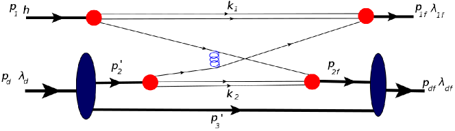
Figure B.1: Typical quark-interchange mechanism of hard $pd\rightarrow pd$ scattering.

The Feynman amplitude for this $pd\rightarrow pd$ scattering can be written as follows:

$$\mathcal{M}_{pd}=$$

$$N1: \int\bar{u}(p_{1f},\lambda_{1f})(-i)\Gamma_{n1}^{\dagger}\frac{i(\not{p}_{1f}-\not{k}_{1}+m_{q})}{(p_{1f}-k_{1})^{2}-m_{q}^{2}+i\epsilon}\frac{iS(k_{1})}{k_{1}^{2}-m_{s}^{2}+i\epsilon}[-igT_{c}^{\beta}\gamma_{\mu}]$$

$$\times\frac{i(\not{p_{1}}-\not{k_{1}}+m_{q})}{(p_{1}-k_{1})^{2}-m_{q}^{2}+i\epsilon}i\Gamma_{n1}u(p_{1},\lambda_{1})\frac{d^{4}k_{1}}{(2\pi)^{4}}$$

$$D-N2: \int\chi_{df}^{\dagger}(-i)\Gamma_{DNN}^{\dagger}\frac{i(\not{p}_{2f}+m)}{p_{2f}^{2}-m_{N}^{2}+i\epsilon}\bar{u}(p_{2f},\lambda_{2f})(-i)\Gamma_{n2f}^{\dagger}\frac{i(\not{p}_{2f}-\not{k}_{2}+m_{q})}{(p_{2f}-k_{2})^{2}-m_{q}^{2}+i\epsilon}$$

$$\times\frac{i(\not{p_{3}}^{\prime}+m)}{p_{3}^{\prime 2}-m_{N}^{2}+i\epsilon}\frac{iS(k_{2})}{k_{2}^{2}-m_{s}^{2}+i\epsilon}[-igT_{c}^{\alpha}\gamma_{\nu}]\frac{i(\not{p_{2}}^{\prime}-\not{k_{2}}+m_{q})}{(p_{2}^{\prime}-k_{2})^{2}-m_{q}^{2}+i\epsilon}i\Gamma_{n2^{\prime}}u(p_{2}^{\prime},\lambda_{2}^{\prime})$$

$$\times\frac{i(\not{p}_{2}^{\prime}+m)}{p_{2}^{\prime 2}-m_{N}^{2}+i\epsilon}i\Gamma_{DNN}\chi_{d}\frac{d^{4}k_{2}}{(2\pi)^{4}}\frac{d^{4}p_{3}^{\prime}}{(2\pi)^{4}}$$

$$g: \frac{id_{\mu\nu}\delta_{\alpha\beta}}{q_{q}^{2}}.$$ (B-2)

The following derivations are analogous to that of Eq. (III), where we identify the parts associated with the deuteron wave function as well as with the quark wave functions of nucleons and perform integrations corresponding to the on-shell conditions for the spectator nucleon in the deuteron and spectator quark-gluon states in the nucleons. We first consider the expression for ${\bf N1}$, for which, performing derivations similar to those for the $N1$ term in Eq. (III) and using the definition of the quark wave function of the nucleon according to Eq. (A-17) one obtains

$$N1:=\sum_{\begin{subarray}{c}\lambda_{1}\\ \eta_{1},\eta_{1f}\end{subarray}} -i\int\frac{\Psi_{n1f}^{\dagger\lambda_{1f};\eta_{1f}}(x_{s1},k_{1\perp},p_{1f\perp})}{1-x_{s1}}\bar{u}_{q}(p_{1f}-k_{1},\eta_{1f})u_{q}(p_{1}-k_{1},\eta_{1})\Big{[}-igT_{c}^{\beta}\gamma_{\mu}\Big{]}$$ (B-3)

$$\times\frac{\Psi_{n1}^{\lambda_{1};\eta_{1}}(x_{1},k_{1\perp},p_{1\perp})}{1-x_{1}}\frac{1}{2}\dfrac{dx_{1}}{x_{1}}\dfrac{d^{2}k_{1\perp}}{(2\pi)^{3}}.$$

With similar derivations in the ${\bf D-N2}$ part and using, in addition to the quark wave function of nucleon, the deuteron light-front wave function defined in Eq. (A-9) one obtains

$$D-N2= \sum_{\begin{subarray}{c}\lambda_{d},\lambda_{2f},\lambda_{2}^{\prime},\lambda_{3}^{\prime}\\ \eta_{2}^{\prime},\eta_{2f}\end{subarray}}-i\int\frac{\Psi_{df}^{\dagger\lambda_{df}:\lambda_{3}^{\prime},\lambda_{2f}}(\alpha_{3}^{\prime}/\gamma_{d},p_{df\perp},p_{3\perp}^{\prime})}{1-\alpha_{3}^{\prime}/\gamma_{d}}\bar{u}_{q}(p_{2f}-k_{2},\eta_{2f})$$ (B-4)

$$\times\frac{\Psi^{\dagger\lambda_{2f};\eta_{2f}}_{n2f}(x_{s2},k_{2\perp},p_{2f\perp})}{1-x_{s2}}[-igT_{c}^{\alpha}\gamma_{\nu}]\frac{\Psi_{d}^{\lambda_{d}:\lambda_{2}^{\prime},\lambda_{3}^{\prime}}(\alpha_{3}^{\prime},p_{d\perp},p_{3\perp}^{\prime})}{1-\alpha_{3}^{\prime}}u_{q}(p_{2}^{\prime}-k_{2},\eta_{2}^{\prime})$$

$$\times\frac{\Psi_{n2^{\prime}}^{\lambda_{2}^{\prime};\eta_{2}^{\prime}}(x_{2}^{\prime},k_{2\perp},p_{2\perp}^{\prime})}{1-x_{2}^{\prime}}\frac{1}{2}\frac{dx_{2}^{\prime}}{x_{2}^{\prime}}\frac{d^{2}k_{2\perp}}{(2\pi)^{3}}\frac{d\alpha_{3}^{\prime}}{\alpha_{3}^{\prime}}\frac{d^{2}p_{3\perp}^{\prime}}{2(2\pi)^{3}}.$$

Combining Eqs.(B-3) and (B-4) for the amplitude of $pd\rightarrow pd$ scattering, one arrives at

$$\mathcal{M}_{pd}^{\lambda_{df},\lambda_{1f};\lambda_{d},\lambda_{1}}=\sum_{\begin{subarray}{c}(\lambda_{2f})(\lambda_{1},\lambda_{d})(\lambda_{2}^{\prime},\lambda_{3}^{\prime})\\ (\eta_{1f},\eta_{2f})(\eta_{1},\eta_{2}^{\prime})\end{subarray}}\int\frac{\Psi_{df}^{\dagger\lambda_{df}:\lambda_{3}^{\prime},\lambda_{2f}}(\alpha_{3}^{\prime}/\gamma_{d},p_{df\perp},p_{3\perp}^{\prime})}{1-\alpha_{3}^{\prime}/\gamma_{d}}\Bigg{\{}\frac{\Psi^{\dagger\lambda_{2f};\eta_{2f}}_{n2f}(x_{s2},k_{2\perp},p_{2f\perp})}{1-x_{s2}}$$

$$\times\bar{u}_{q}(p_{2f}-k_{2},\eta_{2f})[-igT_{c}^{\alpha}\gamma_{\nu}]u_{q}(p_{1}-k_{1},\eta_{1})\frac{\Psi_{n1}^{\lambda_{1};\eta_{1}}(x_{1},k_{1\perp},p_{1\perp})}{1-x_{1}}\Bigg{\}}_{1}G^{\mu\nu}(r)$$

$$\times\Bigg{\{}\frac{\Psi_{n1f}^{\dagger\lambda_{1f};\eta_{1f}}(x_{s1},k_{1\perp},p_{1f\perp})}{1-x_{s1}}\bar{u}_{q}(p_{1f}-k_{1},\eta_{1f})[-igT_{c}^{\beta}\gamma_{\mu}]u_{q}(p_{2}^{\prime}-k_{2},\eta_{2}^{\prime})\frac{\Psi_{n2^{\prime}}^{\lambda_{2}^{\prime};\eta_{2}^{\prime}}(x_{2}^{\prime},k_{2\perp},p_{2\perp}^{\prime})}{1-x_{2}^{\prime}}\Bigg{\}}_{2}$$

$$\times\frac{\Psi_{d}^{\lambda_{d}:\lambda_{2}^{\prime},\lambda_{3}^{\prime}}(\alpha_{3}^{\prime},p_{d\perp},p_{3\perp}^{\prime})}{1-\alpha_{3}^{\prime}}\frac{1}{2}\dfrac{dx_{1}}{x_{1}}\dfrac{d^{2}k_{1\perp}}{(2\pi)^{3}}\frac{1}{2}\frac{dx_{2}^{\prime}}{x_{2}^{\prime}}\frac{d^{2}k_{2\perp}}{(2\pi)^{3}}\frac{d\alpha_{3}^{\prime}}{\alpha_{3}^{\prime}}\frac{d^{2}p_{3\perp}^{\prime}}{2(3\pi)^{3}}.$$ (B-5)

APPENDIX C: Relating the Light-Front and Non-Relativistic Wave Functions

To obtain the relation between light-front and nonrelativistic nuclear wave functions in the small-momentum limit, we consider the fact that the light-front nuclear wave function is normalized based on baryonic number conservation (see, e.g., Refs.Frankfurt:1985ui ; srcrev ; Cosyn:2010ux ), while the nonrelativistic (Schroedinger) wave function is normalized as $\int|\Psi_{A}(p)|^{2}d^{3}p=1$.

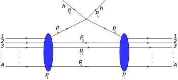
Figure C.1: Hadronic probe to see baryons in a nucleus.

To obtain the normalization condition based on baryonic number conservation, we consider a $h+A\rightarrow h+A$ scattering in forward direction in which $h$ probes the constituent baryons in the nucleus $A$ (see Fig. C.1). In the figure we assign $p_{i}$ to be the four-momentum of the nucleus while $p_{1},p_{2},\cdots,p_{A}$ are four-momenta of constituent nucleons such that $p_{1}+p_{2}+\cdots+p_{A}=p_{i}$. For the diagram of Fig. C.1, applying the Feynman rules one obtains

$$\mathcal{M}_{hA} =\sum_{N}\int\chi_{A}^{\dagger}\Gamma_{A}^{\dagger}\frac{\not{p}_{1}+m}{p_{1}^{2}-m_{N}^{2}+i\epsilon}\hat{M}_{hN}\frac{\not{p}_{A}+m}{p_{A}^{2}-m_{N}^{2}+i\epsilon}\cdots\frac{\not{p}_{2}+m}{p_{2}^{2}-m_{N}^{2}+i\epsilon}\frac{\not{p}_{1}+m}{p_{1}^{2}-m_{N}^{2}+i\epsilon}\Gamma_{A}\chi_{A}$$ (C-1)

$$\times\frac{d^{4}p_{2}}{(2\pi)^{4}}\frac{d^{4}p_{3}}{(2\pi)^{4}}\cdots\frac{d^{4}p_{A}}{(2\pi)^{4}},$$

where we sum over all the possible nucleons that can be probed and ${\hat{M}}_{hN}$ represents the effective vertex of the hadron-nucleon interaction. We use the sum rule for the spinors and also integrate by the minus component of the momenta using the scheme given in Eq. (A-6), to obtain

$$\mathcal{M}_{hA} = \sum_{N}\sum_{\lambda_{1},\lambda_{2},\cdots\lambda_{A}}\int\chi_{A}^{\dagger}\Gamma_{X}^{\dagger}\frac{u(p_{1},\lambda_{1})\bar{u}(p_{1},\lambda_{1})}{p_{1+}\big{(}p_{1-}-\frac{m_{N}^{2}+p_{1\perp}^{2}}{p_{1+}}\big{)}}\hat{M}_{hN}u(p_{A},\lambda_{A})\bar{u}(p_{A},\lambda_{A})\cdots$$ (C-2)

$$\times u(p_{3},\lambda_{3})\bar{u}(p_{3},\lambda_{3})u(p_{2},\lambda_{2})\bar{u}(p_{2},\lambda_{2})\frac{u(p_{1},\lambda_{1})\bar{u}(p_{1},\lambda_{1})}{p_{1+}\big{(}p_{1-}-\frac{m_{N}^{2}+p_{1\perp}^{2}}{p_{1+}}\big{)}}\Gamma_{A}\chi_{A}$$

$$\times\frac{dp_{2+}}{p_{2+}}\frac{d^{2}p_{2\perp}}{2(2\pi)^{3}}\frac{dp_{3+}}{p_{3+}}\frac{d^{2}p_{3\perp}}{2(2\pi)^{3}}\cdots\frac{dp_{A+}}{p_{A+}}\frac{d^{2}p_{A\perp}}{2(2\pi)^{3}},$$

where the $\lambda_{j}$ denote the helicities of the nucleon with momentum $p_{j}$. Considering the transverse momentum of the nucleus $A$ to be zero, we note that

$$p_{1-}-\frac{m_{N}^{2}+p_{1\perp}^{2}}{p_{1+}}=p_{i-}-p_{2-}-p_{3-}-\cdots-p_{A-}-\frac{m_{N}^{2}+p_{1\perp}^{2}}{p_{1+}}$$

$$=\frac{1}{p_{i+}}\Big{[}m_{N}^{2}-\frac{m_{N}^{2}+p_{2\perp}^{2}}{\beta_{2}}-\frac{m_{N}^{2}+p_{3\perp}^{2}}{\beta_{3}}-\cdots-\frac{m_{N}^{2}+p_{A\perp}^{2}}{\beta_{A}}-\frac{m_{N}^{2}+p_{1\perp}^{2}}{\beta_{1}}\Big{]},$$ (C-3)

where $\beta_{j}=\frac{p_{j+}}{p_{i+}}$ are the light-front momentum fractions of the nucleus $A$ carried by the nucleons $j$ ($j=1,\cdots A$). Introducing the Feynman amplitude for $h+N\rightarrow hN$ as $\mathcal{M}_{hN}=\bar{u}(p_{1},\lambda_{1})\hat{M}_{hN}u(p_{1},\lambda_{1})$ for Eq. (APPENDIX C: Relating the Light-Front and Non-Relativistic Wave Functions) one obtains

$$\mathcal{M}_{hA} =\sum_{N}\sum_{\lambda_{1},\lambda_{2},\cdots\lambda_{A}}\int\chi_{A}^{\dagger}\Gamma_{A}^{\dagger}\frac{u(p_{1},\lambda_{1})u(p_{2},\lambda_{2})u(p_{3},\lambda_{3})\cdots u(p_{A},\lambda_{A})}{\frac{p_{1+}}{p_{i+}}\Big{[}m_{N}^{2}-\frac{m_{N}^{2}+p_{2\perp}^{2}}{\beta_{2}}-\frac{m_{N}^{2}+p_{3\perp}^{2}}{\beta_{3}}-\cdots-\frac{m_{N}^{2}+p_{A\perp}^{2}}{\beta_{A}}\Big{]}}\mathcal{M}_{hN}$$ (C-4)

$$\times\frac{\bar{u}(p_{1},\lambda_{1})\bar{u}(p_{2},\lambda_{2})\bar{u}(p_{A},\lambda_{A})}{\frac{p_{1+}}{p_{i+}}\Big{[}m_{N}^{2}-\frac{m_{N}^{2}+p_{2\perp}^{2}}{\beta_{2}}-\frac{m_{N}^{2}+p_{3\perp}^{2}}{\beta_{3}}-\cdots-\frac{m_{N}^{2}+p_{A\perp}^{2}}{\beta_{A}}\Big{]}}\Gamma_{A}\chi_{A}\prod_{k=2}^{A}\frac{d\beta_{k}}{\beta_{k}}\frac{d^{2}p_{k\perp}}{2(2\pi)^{3}}.$$

Using the generalization of Eqs.(A-4) and (A-9) for light-front nuclear wave function of nucleus $A$, the above equation reduces to

$$\mathcal{M}_{hA} =\sum_{N}\sum_{\lambda_{1},\lambda_{2},...\lambda_{A}}\int\frac{\Psi_{A}^{LC\dagger}(\beta_{2},\beta_{3},...\beta_{A},p_{2\perp},p_{3\perp}...p_{A\perp},\lambda_{2},\lambda_{3},...\lambda_{A})}{\beta_{1}}\mathcal{M}_{hN}$$ (C-5)

$$\times\frac{\Psi_{A}^{LC}(\beta_{2},\beta_{3},...\beta_{A},p_{2\perp},p_{3\perp}...p_{A\perp},\lambda_{2},\lambda_{3},...\lambda_{A})}{\beta_{1}}\prod_{k=2}^{A}\frac{d\beta_{k}}{\beta_{k}}\frac{d^{2}p_{k\perp}}{2(2\pi)^{3}}.$$

We now make use of the optical theorem, according to which

$$\text{Im }\mathcal{M}_{hA}=s_{hA}\sigma_{hA}\text{ and }\text{Im }\mathcal{M}_{hN}=s_{hN}\sigma_{hN},$$ (C-6)

where $s_{hA}=(p_{h}+p_{i})^{2}$ and $\sigma_{hA}$ is the total cross section of $hA$ scattering. Similarly, $s_{hN}$ and $\sigma_{hN}$ are invariant energy and total cross section for $hN$ scattering. The conservation of baryon number allows us to relate $\sigma_{hA}=A\sigma_{hN}$. Using this relation together with Eq. (C-6) in Eq. (C-5), one obtains

$$\int\frac{\left|\Psi_{A}^{LC}(\beta_{2},\beta_{3},...\beta_{A},p_{2\perp},p_{3\perp}...p_{A\perp},\lambda_{2},\lambda_{3},...\lambda_{A})\right|^{2}}{\beta_{1}^{2}}\frac{s_{hN}}{s_{hA}}\prod_{k=2}^{A}\frac{d\beta_{k}}{\beta_{k}}\frac{d^{2}p_{k\perp}}{2(2\pi)^{3}}=1.$$ (C-7)

To obtain the relation of light-front wave function to the nonrelativistic wave function in the small-momentum limit, we note that in such limit $\beta_{k}=\frac{E_{k}+p_{k}^{z}}{p_{i+}}\approx 1+\frac{p_{k}^{z}}{m_{N}}$ thus $\frac{d\beta_{k}}{\beta_{k}}=\frac{dp_{k}^{z}}{m_{N}}$. Furthermore, in the high energy limit of the hadronic probe in which large momentum of the hadrons points in the $-\hat{z}$ direction, $s_{hA}\approx p_{h-}p_{A+}$ and $s_{hN}\approx p_{h-}p_{N+}$ resulting in

$$\frac{s_{hN}}{s_{hA}}=\frac{p_{N+}}{p_{A+}}=\frac{\beta_{1}}{A}.$$ (C-8)

Applying all these approximations in Eq. (C-7) one obtains

$$\int\frac{\left|\Psi_{A}^{LC}(\beta_{2},\beta_{3},...\beta_{A},p_{2\perp},p_{3\perp}...p_{A\perp},\lambda_{2},\lambda_{3},...\lambda_{A})\right|^{2}}{1/A}\frac{1}{m_{N}^{A-1}[2(2\pi)^{3}]^{A-1}}\prod_{k=2}^{A}d^{3}p_{k}=1.$$ (C-9)

Next we compare the above expression with the normalization condition for the nonrelativistic Schroedinger wave function:

$$\int\left|\Psi_{A}^{NR}(\vec{p}_{1},\vec{p}_{2},...\vec{p}_{A})\right|^{2}\prod_{k=2}^{A}d^{3}p_{k}=1,$$ (C-10)

where $\vec{p}_{1}=\vec{p}_{i}-\vec{p}_{2}-\cdots-\vec{p}_{A}$. This comparison allows us to relate the light-front nuclear wave function and the Schroedinger wave function in the following form:

$$\Psi_{X}^{LC}(\beta_{1},\beta_{2},...,p_{1\perp},p_{2\perp}...)=\frac{1}{\sqrt{A}}\big{[}m_{N}2(2\pi)^{3}\big{]}^{\frac{A-1}{2}}\Psi_{X}^{NR}(\vec{p}_{1},\vec{p}_{2},...).$$ (C-11)

References

- (1) S. J. Brodsky and G. R. Farrar, Phys. Rev. Lett. 31, 1153 (1973).
- (2) V. A. Matveev, R. M. Muradian and A. N. Tavkhelidze, Lett. Nuovo Cim. 7, 719 (1973).
- (3) S. J. Brodsky and B. T. Chertok, Phys. Rev. D 14, 3003 (1976).
- (4) J. Napolitano et al., Phys. Rev. Lett. 61, 2530 (1988).
- (5) S. J. Freedman et al., Phys. Rev. C 48, 1864 (1993).
- (6) J. E. Belz et al., Phys. Rev. Lett. 74, 646 (1995). doi:10.1103/PhysRevLett.74.646
- (7) C. Bochna et al. [E89-012 Collaboration], Phys. Rev. Lett. 81, 4576 (1998).
- (8) E. C. Schulte, A. Ahmidouch, C. S. Armstrong, J. Arrington, R. Asaturyan, S. Avery, O. K. Baker and D. H. Beck et al., Phys. Rev. Lett. 87, 102302 (2001).
- (9) E. C. Schulte et al., Phys. Rev. C 66, 042201 (2002).
- (10) M. Mirazita et al. [CLAS Collaboration], Phys. Rev. C 70, 014005 (2004).
- (11) P. Rossi et al. [CLAS Collaboration], Phys. Rev. Lett. 94, 012301 (2005).
- (12) K. Wijesooriya et al. [Jefferson Lab Hall A Collaboration], Phys. Rev. Lett. 86, 2975 (2001).
- (13) F. Adamian et al., Eur. Phys. J. A 8, 423 (2000).
- (14) X. Jiang et al. [Jefferson Lab Hall A Collaboration], Phys. Rev. Lett. 98, 182302 (2007).
- (15) N. Zachariou et al. [CLAS Collaboration], Phys. Rev. C 91, no. 5, 055202 (2015).
- (16) S. J. Brodsky, L. Frankfurt, R. A. Gilman, J. R. Hiller, G. A. Miller, E. Piasetzky, M. Sargsian and M. Strikman, Phys. Lett. B 578, 69 (2004).
- (17) I. Pomerantz et al. [JLab Hall A Collaboration], Phys. Lett. B 684, 106 (2010).
- (18) I. Pomerantz et al. [CLAS and Hall-A and Hall-B Collaborations], Phys. Rev. Lett. 110, no. 24, 242301 (2013).
- (19) L. L. Frankfurt, G. A. Miller, M. M. Sargsian and M. I. Strikman, Phys. Rev. Lett. 84, 3045 (2000).
- (20) L. L. Frankfurt, G. A. Miller, M. M. Sargsian and M. I. Strikman, Nucl. Phys. A 663-664, 349 (2000).
- (21) M. M. Sargsian, AIP Conf. Proc. 1056, 287 (2008).
- (22) M. M. Sargsian, Phys. Lett. B 587, 41 (2004).
- (23) M. M. Sargsian and C. Granados, Phys. Rev. C 80, 014612 (2009).
- (24) C. G. Granados and M. M. Sargsian, Phys. Rev. C 83, 054606 (2011).
- (25) R. J. Holt, Phys. Rev. C 41, 2400 (1990).
- (26) L. L. Frankfurt, M. M. Sargsian and M. I. Strikman, Phys. Rev. C 56, 1124 (1997).
- (27) M. M. Sargsian, Int. J. Mod. Phys. E 10, 405 (2001).
- (28) M. M. Sargsian, Phys. Rev. C 82, 014612 (2010).
- (29) R. A. Gilman and F. Gross, J. Phys. G 28, R37 (2002) doi:10.1088/0954-3899/28/4/201.
- (30) B.L. Berman, G. Audit, and P. Corvisiero, ”Photoreactions on 3He”, Jefferson Lab Experiment E93-044, (1993).
- (31) V. Isbert et al., Nucl. Phys. A 578, 525 (1994).
- (32) Yordanka Illieave, Private Communication.
- (33) N. E. Booth, C. Dolnick, R. J. Esterling, J. Parry, J. Scheid and D. Sherden, Phys. Rev. D 4, 1261 (1971).
- (34) E. T. Boschitz et al., Phys. Rev. C 6, 457 (1972).
- (35) E. Guelmez et al., Phys. Rev. C 43, 2067 (1991).
- (36) E. Winkelmann, P. R. Bevington, M. W. Mcnaughton, H. B. Willard, F. H. Cverna, E. P. Chamberlin and N. S. P. King, Phys. Rev. C 21, 2535 (1980).
- (37) L. Dubal et al., Phys. Rev. D 9, 597 (1974).
- (38) A. Nogga, A. Kievsky, H. Kamada, W. Gloeckle, L. E. Marcucci, S. Rosati and M. Viviani, Phys. Rev. C 67, 034004 (2003).
- (39) R. B. Wiringa, V. G. J. Stoks and R. Schiavilla, Phys. Rev. C 51, 38 (1995).
- (40) M. M. Sargsian, T. V. Abrahamyan, M. I. Strikman and L. L. Frankfurt, Phys. Rev. C 71, 044615 (2005).
- (41) L. L. Frankfurt and M. I. Strikman, Phys. Rept. 76, 215 (1981).
- (42) A. J. Freese, M. M. Sargsian and M. I. Strikman, Eur. Phys. J. C 75, no. 11, 534 (2015).
- (43) O. Artiles and M. M. Sargsian, Phys. Rev. C 94, 064318 (2016).
- (44) L. L. Frankfurt and M. I. Strikman, Phys. Lett. B 183, 254 (1987).
- (45) L. Frankfurt, M. Sargsian and M. Strikman, Int. J. Mod. Phys. A 23, 2991 (2008).
- (46) W. Cosyn and M. Sargsian, Phys. Rev. C 84, 014601 (2011).