Slave Boson Theory of Orbital Differentiation with Crystal Field Effects:
Application to UO₂

Abstract

We derive an exact operatorial reformulation of the rotational invariant slave boson method and we apply it to describe the orbital differentiation in strongly correlated electron systems starting from first principles. The approach enables us to treat strong electron correlations, spin-orbit coupling and crystal field splittings on the same footing by exploiting the gauge invariance of the mean-field equations. We apply our theory to the archetypical nuclear fuel UO₂, and show that the ground state of this system displays a pronounced orbital differention within the $5f$ manifold, with Mott localized $\Gamma_{8}$ and extended $\Gamma_{7}$ electrons.

Orbital differentiation, where states with different orbital character exhibit different levels of correlation, is a pervasive phenomena in condensed matter systems Koga et al. (2004); Anisimov et al. (2002); de’ Medici et al. (2009); Lanatà et al. (2013), which gives rise to multiple functionalities in strongly correlated multiorbital systems. In all known Mott systems in nature only a fraction of electrons form localized magnetic moments, while the other electronic states are extended (but away from the Fermi level). These systems are commonly called “selective Mott insulators”, and the transition into these states is called “orbitally selective Mott transition”. Understanding the mechanism driving the selection process is a fundamental question in condensed matter. This issue is especially nontrivial to address in low-symmetry $5f$ electron systems, where the competition between inter- and intra-orbital interactions, the crystal field splittings (CFS) and the spin-orbit coupling (SOC) is very complicated, as none of these energy scales is negligible. Orbital differentiation is also a key issue in the presence of disorder Dobrosavljević et al. (2012); Marianetti et al. (2004) and/or charge ordering (Wigner-Mott transitions Camjayi et al. (2008)), where only a fraction of the electrons Mott-localize. Addressing these issues quantitatively and in an unbiased “ab-initio” fashion is very challenging. In this work we address the orbital differentiation problem from an ab-initio perspective using the rotationally invariant slave boson (RISB) mean-field theory Kotliar and Ruckenstein (1986); Lechermann et al. (2007); Li et al. (1989). As we demonstrate, this method can be derived from an exact operatorial reformulation of the many-body problem, which reproduces the Gutzwiller approximation Gutzwiller (1965) at the mean-field level Bünemann and Gebhard (2007); Lanatà et al. (2008) and constitutes a starting point to calculate further corrections. By exploiting the gauge symmetry of the RISB theory, we build efficient systematic algorithms which enable us to solve the mean-field equations and elucidate the pattern of orbital differentiation even in low-symmetry $5f$ electron systems. We apply this method to UO₂ Yin et al. (2011) (the most widely used nuclear fuel), and provide new insight into the role of the CFS in the orbital differentiation and the nature of the chemical bonds in this material.

The multi-band Hubbard model:— Let us consider a generic multi-band Hubbard model:

$$\vspace{-0.035cm}\hat{H}\!=\!\sum_{k}\!\sum_{ij=1,..,n_{a}}\,\sum_{\alpha=1,..,M_{i}}\sum_{\beta=1,..,M_{j}}\!\!\!\!\epsilon^{\alpha\beta}_{k,ij}\,c^{\dagger}_{ki\alpha}c^{\phantom{\dagger}}_{kj\beta}\!+\!\hat{H}^{\text{loc}}\!,\vspace{-0.035cm}$$ (1)

where $k$ is the momentum conjugate to the unit-cell label $R$, the $n_{a}$ atoms within the unit cell are labeled by $i,j$, and the spin-orbitals are labeled by $\alpha,\beta$. As in Refs. Lechermann et al., 2007; Lanatà et al., 2015, the local interaction and the on-site energies are both included within the definition of:

$$\vspace{-0.035cm}\hat{H}^{\text{loc}}\equiv\sum_{Ri}\sum_{AB}\big{[}H^{\text{loc}}_{i}\big{]}_{AB}\,|A,Ri\rangle\langle B,Ri|\,,\vspace{-0.035cm}$$ (2)

where $|A,Ri\rangle$ are local Fock states:

$$\vspace{-0.035cm}|A,Ri\rangle=[c^{\dagger}_{Ri1}]^{\nu_{1}(A)}\!\!\!\!\!\!.\,.\,.\;[c^{\dagger}_{RiM_{i}}]^{\nu_{M_{i}}(A)}\,|0\rangle\,,\vspace{-0.035cm}$$ (3)

and $A=1,..,2^{M_{i}}$ runs over all of the possible lists of occupation numbers $\{\nu_{1}(A),..,\nu_{M_{i}}(A)\}$. In particular, in this work we have used the Slater-Condon parametrization of the on-site interaction Anisimov et al. (1997a).

Slave Boson reformulation:— Here we derive the RISB gauge theory and show that it constitutes an exact reformulation of the generic Hubbard system defined above. As in Ref. Lechermann et al., 2007, we introduce a new set of fermionic modes $\{f^{\phantom{\dagger}}_{Ria}|a=1,..,M_{i}\}$, that we call quasi-particle operators. Furthermore, we introduce a bosonic mode $\Phi^{\phantom{\dagger}}_{RiAn}$ for each couple of fermionic local multiplets $(|A,Ri\rangle,|n,Ri\rangle)$ having equal number of electrons, i.e., $N_{A}\equiv\sum_{a=1}^{M_{i}}\nu_{a}(A)=N_{n}\equiv\sum_{a=1}^{M_{i}}\nu_{a}(n)$. Applying the algebra generated by $\{\Phi^{\dagger}_{RiAn}\}$ and $\{f^{\dagger}_{Ria}\}$ to the vacuum $|0\rangle$ generates a new Fock space $\mathcal{H}_{\text{SB}}$. We define “physical Hilbert space” the subspace $h_{\text{SB}}$ of $\mathcal{H}_{\text{SB}}$ satisfying the following equations (Gutzwiller constraints):

$$\vspace{-0.035cm}K^{0}_{Ri}\! \equiv \!\sum_{An}\Phi^{\dagger}_{RiAn}\!\Phi^{\phantom{\dagger}}_{RiAn}-\hat{I}\!=\!0$$ (4)

$$K_{Riab}\! \equiv \!f^{\dagger}_{Ria}f^{\phantom{\dagger}}_{Rib}\!-\!\sum_{Anm}[F^{\dagger}_{ia}F^{\phantom{\dagger}}_{ib}]_{mn}\,\Phi^{\dagger}_{RiAn}\!\Phi^{\phantom{\dagger}}_{RiAm}\!=\!0\,,\leavevmode\nobreak\ \leavevmode\nobreak\ \leavevmode\nobreak\ \leavevmode\nobreak\ \vspace{-0.03cm}$$ (5)

where $\hat{I}$ is the identity, $\left[F_{ia}\right]_{nm}\equiv\langle n,Ri|\,f^{\phantom{\dagger}}_{Ria}\,|m,Ri\rangle$, and $|n,Ri\rangle$ and $|m,Ri\rangle$ are Fock states constructed as in Eq. (3), but using the quasi-particle operators $f^{\phantom{\dagger}}_{Ria}$.

In Ref. Lanatà et al., 2015 it was shown that the following Hamiltonian is an exact representation of $\hat{H}$ within $h_{\text{SB}}$:

$$\vspace{-0.035cm}\underline{\hat{H}}=\!\!\!\sum_{kij\alpha\beta}\!\!\!\epsilon^{\alpha\beta}_{k,ij}\,\underline{c}^{\dagger}_{ki\alpha}\underline{c}^{\phantom{\dagger}}_{kj\beta}+\!\!\sum_{RiAB}\!\![H_{i}^{\text{loc}}]_{AB}\!\sum_{n}\Phi^{\dagger}_{RiAn}\!\Phi^{\phantom{\dagger}}_{RiBn},\vspace{-0.035cm}$$ (6)

where $\underline{c}^{\dagger}_{Ri\alpha}\equiv\sum_{a}\hat{\mathcal{R}}_{Ria\alpha}\,f^{\dagger}_{Ria}$, and the operators

$$\vspace{-0.035cm}\hat{\mathcal{R}}_{Ria\alpha}=\sum_{AB}\sum_{nm}\frac{[F^{\dagger}_{i\alpha}]_{AB}[F^{\dagger}_{ia}]_{nm}}{\sqrt{N_{A}(M_{i}-N_{B})}}\,\Phi^{\dagger}_{RiAn}\Phi^{\phantom{\dagger}}_{RiBm}\vspace{-0.035cm}$$ (7)

are such that $\underline{c}^{\dagger}_{Ri\alpha}$ are a representation in $h_{\text{SB}}$ of $c^{\dagger}_{Ri\alpha}$. A remarkable property of $\underline{\hat{H}}$ is that it is invariant with respect to the gauge Lie group generated by the Gutzwiller constraint operators $K_{Riab}$, see Eq. (5):

$$\vspace{-0.035cm}e^{i\sum_{Riab}\theta_{ab}K_{Riab}}\,\underline{\hat{H}}\,e^{-i\sum_{Riab}\theta_{ab}K_{Riab}}=\underline{\hat{H}}\;\,\forall\,\theta=\theta^{\dagger}\,.\vspace{-0.035cm}$$ (8)

In fact, Eq. (8) does not hold only within the subspace $h_{\text{SB}}$ (which would be a trivial consequence of Eq. (5)), but in the entire RISB Fock space $\mathcal{H}_{\text{SB}}$ sup .

Operatorial formulation of RISB theory:— The operators $\hat{\mathcal{R}}_{Ria\alpha}$ defined above are constructed in such a way that $\underline{c}^{\dagger}_{Ri\alpha}$ are a representation in the physical RISB subspace of the corresponding original fermionic operators $c^{\dagger}_{Ri\alpha}$. However, this construction is not unique. In particular, Eq. (7) can be modified as follows:

$$\vspace{-0.035cm}\hat{\mathcal{R}}_{Ria\alpha}\!\!=:\!\sum_{AB}\!\sum_{nm}\!\!\frac{[F^{\dagger}_{i\alpha}]_{AB}[F^{\dagger}_{ia}]_{nm}}{\sqrt{N_{A}(M_{i}-N_{B})}}\,\Phi^{\dagger}_{RiAn}[\hat{1}\!+\!\hat{X}_{AB}]\,\Phi^{\phantom{\dagger}}_{RiBm}\!:\vspace{-0.035cm}$$ (9)

where “$:$” indicates the normal ordering Schönhammer (1990), and $\hat{X}_{AB}$ is any normally-ordered algebraic combination of bosonic ladder operators such that each term contains at least 2 modes. In fact, since $\hat{X}_{AB}$ is normally-ordered and the physical RISB states contain only one boson by construction, see Eq. (4), the matrix elements of Eqs. (7) and (9) are independent of $\hat{X}_{AB}$ within $h_{\text{SB}}$.

Of course, any choice of $\hat{X}_{AB}$ in Eq. (9) would be equivalent if we were able to solve $\underline{\hat{H}}$ exactly. However, this choice affects the RISB mean-field approximation (that we are going to introduce below). Interestingly, it is possible to construct $\hat{X}_{AB}$ in such a way that: (i) the RISB mean-field theory is exact for any uncorrelated Hubbard Hamiltonian, and (ii) the invariance property [Eq. (8)] of $\underline{\hat{H}}$ with respect to the gauge group remains valid. To the best of our knowledge, this operatorial construction, which is derived in the supplemental material of this work sup , was not provided in any previous work.

RISB mean-field theory:— At zero temperature, the RISB mean-field theory consists in minimizing the expectation value of $\underline{\hat{H}}$ with respect to $|\Psi_{\text{MF}}\rangle=|\Psi_{0}\rangle\otimes|\phi\rangle$, where $|\Psi_{0}\rangle$ is a Slater determinant constructed with the quasi-particle operators $f^{\phantom{\dagger}}_{Ria}$, $|\phi\rangle$ is a bosonic coherent state, and the Gutzwiller constraints, see Eqs (4) and (5), are enforced only in average.

It can be verified that taking the expectation value of Eqs. (4) and (5) with respect to $|\Psi_{\text{MF}}\rangle$ gives:

$$\vspace{-0.035cm}\mathrm{Tr}\big{[}\phi^{\dagger}_{i}\phi^{\phantom{\dagger}}_{i}\big{]}\! = \!1\;\forall\,i$$ (10)

$$\left[\Delta_{pi}\right]_{ab}\!\equiv\!\mathrm{Tr}\big{[}\phi^{\dagger}_{i}\phi^{\phantom{\dagger}}_{i}F^{\dagger}_{ia}F^{\phantom{\dagger}}_{ib}\big{]}\! = \!\langle\Psi_{0}|\,\!f^{\dagger}_{Ria}f^{\phantom{\dagger}}_{Rib}\!\,|\Psi_{0}\rangle\;\forall\,i\,,\vspace{-0.035cm}$$ (11)

where the matrix elements $[\phi_{i}]_{An}$, which we call “slave boson amplitudes”, are the eigenvalues of the annihilation operators $\Phi_{RiAn}$ with respect to $|\phi\rangle$. Similarly, it can be verified that the expectation value of $\underline{\hat{H}}$ with respect to $|\Psi_{\text{MF}}\rangle$ (normalized to the number of $k$-points $\mathcal{N}$) is given by:

$$\vspace{-0.035cm}\mathcal{E} \equiv \frac{1}{\mathcal{N}}\,\langle\Psi_{\text{MF}}|\,\underline{\hat{H}}\,|\Psi_{\text{MF}}\rangle=\sum_{i}\mathrm{Tr}\big{[}\phi_{i}^{\phantom{\dagger}}\phi_{i}^{\dagger}\,H^{\text{loc}}_{i}\big{]}$$ (12)

$$+ \frac{1}{\mathcal{N}}\sum_{kij}\sum_{ab}\big{[}\mathcal{R}^{\phantom{\dagger}}_{i}\epsilon_{k,ij}\mathcal{R}^{\dagger}_{j}\big{]}_{ab}\langle\Psi_{0}|\,f^{\dagger}_{kia}f^{\phantom{\dagger}}_{kjb}\,|\Psi_{0}\rangle\,,\vspace{-0.035cm}$$

where $[\mathcal{R}_{i}]_{a\alpha}\equiv\langle\phi|\,\hat{\mathcal{R}}_{Ria\alpha}\,|\phi\rangle$ is given by:

$$\vspace{-0.035cm}[\mathcal{R}_{i}]_{a\alpha}=\mathrm{Tr}\big{[}\phi_{i}^{\dagger}F^{\dagger}_{i\alpha}\phi^{\phantom{\dagger}}_{i}F^{\phantom{\dagger}}_{ib}\big{]}\big{[}\Delta_{pi}(1-[\Delta_{pi}])\big{]}^{-\frac{1}{2}}_{ba}\,,\vspace{-0.035cm}$$ (13)

$1$ is the identity matrix, and $\hat{\mathcal{R}}_{Ria\alpha}$ are the renormalization operators represented in Eq. (9), and constructed explicitly in the supplemental material sup . The RISB mean-field theory amounts to minimize Eq. (12) with respect to $|\Psi_{\text{MF}}\rangle$ while fulfilling Eqs. (10) and (11).

Advantages of the gauge invariant formulation:— As shown in the supplemental material sup , the above constrained minimization problem can be conveniently cast — analogously to DMFT Georges et al. (1996); Anisimov et al. (1997b); Lichtenstein and Katsnelson (2000) — as a root problem for the variables $\left(\mathcal{R}_{i},\lambda_{i}\right)$, where $\mathcal{R}_{i}$ were defined in Eq. (13), and $\lambda_{i}$ are matrices of Lagrange multipliers introduced in order to enforce the Gutzwiller constraints [Eq. (11)]. These variables encode the so called “Gutzwiller self energy” of each inequivalent atom, that is defined as:

$$\vspace{-0.035cm}\Sigma_{i}(\omega)\equiv(I-\mathcal{R}^{\dagger}_{i}\mathcal{R}_{i}^{\phantom{\dagger}})(\mathcal{R}^{\dagger}_{i}\mathcal{R}_{i}^{\phantom{\dagger}})^{-1}\,\omega+(\mathcal{R}_{i}^{-1}\lambda_{i}\mathcal{R}_{i}^{\dagger\,-1})\,,\vspace{-0.035cm}$$ (14)

where $Z_{i}\equiv\mathcal{R}_{i}^{\dagger}\mathcal{R}_{i}^{\phantom{\dagger}}$ are matrices of quasi-particle weights. Let us represent formally the above-mentioned root problem as follows:

$$\vspace{-0.035cm}\mathcal{F}[(\mathcal{R}_{1},\lambda_{1}),...,(\mathcal{R}_{n_{a}},\lambda_{n_{a}})]=0\,,\vspace{-0.035cm}$$ (15)

where $n_{a}$ is the number of inequivalent atoms within the unit cell. As shown in the supplemental material sup , each evaluation of $\mathcal{F}$ requires to solve $n_{a}$ impurity models, where the bath has the same dimension of the impurity for each inequivalent atom Lanatà et al. (2015). An important advantage of the present formulation with respect to Ref. Lanatà et al., 2015 is that, by virtue of Eq. (8), Eq. (15) has a manifold of physically equivalent solutions, which are mapped one into the other by the following group of gauge transformations: $\mathcal{R}_{i}\rightarrow u_{i}^{\dagger}(\theta_{i})\,\mathcal{R}_{i}$, $\lambda_{i}\rightarrow u_{i}^{\dagger}(\theta_{i})\,\lambda_{i}\,u_{i}(\theta_{i})$, where $u_{i}(\theta_{i})\equiv e^{i\theta_{i}}$ are generic unitary matrices. This property effectively reduces the dimension of the root problem, which makes the code more stable and speeds up the convergence by reducing substantially the number of evaluations of $\mathcal{F}$ necessary to solve Eq. (15). Remarkably, we found that exploiting the gauge freedom mentioned above is essential in order to study strongly correlated materials where the SOC and the CFS are equally important, which generally makes the structure of $\Sigma_{i}(\omega)$ particularly complex . Further technical details are discussed in the supplemental material sup .

Calculations of UO₂:— UO₂ is widely used as a nuclear fuel. At ambient pressure it is a Mott insulator and crystallizes in a cubic fluorite structure. Given the importance of this material, its electronic structure and energetics have been extensively investigated both experimentally and theoretically, e.g., with DFT+U Geng et al. (2007); Wang et al. (2013); Laskowski et al. (2004) and other single-particle approaches Kudin et al. (2002); Prodan et al. (2006). However, within these techniques it is not possible to address the properties of the paramagnetic state of this material, which is stable above the Néel temperature $T_{\text{N}}\simeq 30.8\,K$ Frazer et al. (1965). Because of this reason, several DMFT studies of paramagnetic UO₂ have been recently performed Yin et al. (2011); Huang et al. (2015); Yin and Savrasov (2008); Kolorenc et al. (2015). A particularly important statement concerning the orbital differentiation of the U-$5f$ electrons was made in Refs. Yin et al. (2011); Huang et al. (2015), where it was observed that the $5f_{5/2}$ states are Mott localized, while the $5f_{7/2}$ states are extended (but gapped). However, these studies did not investigate how this conclusion is influenced by the crystal field effects, which is the main goal of this paper. For this purpose, we perform charge self-consistent LDA+RISB simulations of paramagnetic UO₂ taking fully into account the CFS. As in Ref. Lanatà et al. (2015), we utilize the density functional theory Hohenberg and Kohn (1964) code WIEN2K Blaha et al. (2001) and employ the standard ”fully localized limit” form for the double-counting functional Anisimov et al. (1997a). These calculations would have been prohibitive without the algorithms derived in this work sup .

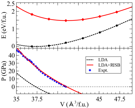
Figure 1: (Color online) Zero temperature LDA and LDA+RISB total energies (upper panel) and corresponding pressure-volume phase diagrams compared with the room-temperature experiments of Ref. Idiri et al. (2004) (lower panel).

As in Ref. Huang et al. (2015), in this work we assume that the Hund’s coupling constant is $J=0.6\,eV$. In the upper panel of Fig. 1 are shown the LDA and LDA+RISB total energies $E(V)$ obtained at zero temperature for $U=10\,eV$ sup . The corresponding pressure (P-V) curves, obtained from $P(V)=-dE/dV$, are shown in the lower panel in comparison with the experimental data of Ref. Idiri et al. (2004) (which were obtained at room temperature). The RISB P-V curve and, in particular, the experimental equilibrium volume $V_{\text{eq}}\simeq 41\,\AA^{3}/\text{f.u.}$, compare remarkably well with the experiments. This favorable comparison with the experiments gives us confidence that our theoretical approach is able to describe the ground-state properties of this material. As shown in the supplemental material sup , the P-V curve (and, in particular, the equilibrium volume) is essentially identical for $U=8\,eV$, which is the value assumed in Ref. Huang et al. (2015). Furthermore, reducing $U$ from $10\,eV$ to $8\,eV$ does not influence appreciably the electronic structure of UO₂ at $V_{\text{eq}}$ .

In order to describe the orbital differentiation in UO₂ taking into account the CFS, it is necessary to decompose the U-$5f$ single-particle space in irreducible representations of the double $O$ point symmetry group Dresselhaus et al. (2007); Wigner (1959) of the U atoms. It can be shown that this repartition consists in: 1 $\Gamma_{6}(2)$ doublet, 2 $\Gamma_{7}(2)$ doublets and 2 $\Gamma_{8}(4)$ quartets . These irreducible representations are generated by the following states:

$$\vspace{-0.035cm}|\Gamma_{6},7/2,\pm\rangle\! = \!\sqrt{5/12}\,|7/2,\pm 7/2\rangle\!+\!\sqrt{7/12}\,|7/2,\mp 1/2\rangle$$

$$|\Gamma_{7},7/2,\pm\rangle\! = \!\mp\sqrt{3/4}\,|7/2,\pm 5/2\rangle\!\pm\!\sqrt{1/4}\,|7/2,\mp 3/2\rangle$$

$$|\Gamma_{8}^{(1)},7/2,\pm\rangle\! = \!\pm\sqrt{7/12}\,|7/2,\pm 7/2\rangle\!\mp\!\sqrt{5/12}\,|7/2,\mp 1/2\rangle$$

$$|\Gamma_{8}^{(2)},7/2,\pm\rangle\! = \!\mp\sqrt{1/4}\,|7/2,\pm 5/2\rangle\!\mp\!\sqrt{3/4}\,|7/2,\mp 3/2\rangle$$

$$|\Gamma_{7},5/2,\pm\rangle\! = \!\sqrt{5/6}\,|5/2,\pm 3/2\rangle\!-\!\sqrt{1/6}\,|5/2,\mp 5/2\rangle$$

$$|\Gamma_{8}^{(1)},5/2,\pm\rangle\! = \!\sqrt{1/6}\,|5/2,\pm 3/2\rangle\!+\!\sqrt{5/6}\,|5/2,\mp 5/2\rangle$$

$$|\Gamma_{8}^{(2)},5/2,\pm\rangle\! = \!|5/2,\pm 1/2\rangle\,,\vspace{-0.035cm}$$ (16)

which are expressed in terms of the conventional basis of eigenstates of the total angular momentum (JJ basis). By virtue of the Schur lemma Wigner (1959), the entries of the U-$5f$ self energy $\Sigma(\omega)$ coupling states belonging to inequivalent irreducible representations are equal to 0. However, the total angular momentum $J^{2}$ is not a good quantum number, as the matrix elements of $\Sigma(\omega)$ coupling the following states are allowed: $|\Gamma_{7},5/2,\pm\rangle$ with $|\Gamma_{7},7/2,\mp\rangle$, $|\Gamma_{8}^{(1)},5/2,\pm\rangle$ with $|\Gamma_{8}^{(2)},7/2,\mp\rangle$ and $|\Gamma_{8}^{(2)},5/2,\pm\rangle$ with $|\Gamma_{8}^{(2)},7/2,\pm\rangle$. Furthermore, the 5/2 and 7/2 states are not degenerate sup . Note that these CFS are present because of the crystal structure, and would not exist if the environment of the $U$ atoms was isotropic.

The main goals of this work are: (1) to show that the CFS affect substantially the electronic structure of UO₂, and (2) to describe and explain the pattern of orbital differentiation of the U-$5f$ electrons in this material.

Table 1: Eigenvalues of the $5f$ quasi-particle matrix $Z$ and corresponding orbital occupations for LDA+RISB calculations at $U=10\,eV$. Theoretical results obtained by taking into account the crystal field splittings and by neglecting them.

w/ CFS	$\Gamma_{8}(4)$	$\Gamma_{7}(2)$	$\Gamma_{8}(4)$	$\Gamma_{7}(2)$	$\Gamma_{6}(2)$
$Z$	$0$	$0.92$	$0.92$	$0.95$	$0.95$
$n$	$1.92$	$0.14$	$0.08$	$0.06$	$0.04$

w/o CFS	$5/2$	$7/2$
$Z$	$0$	$0.96$
$n$	$1.98$	$0.16$

In Table 1 are shown the eigenvalues of the $5f$ quasi-particle matrix $Z=\mathcal{R}^{\dagger}\mathcal{R}$ obtained by taking into account the CFS and the corresponding orbital occupations. The approximate results calculated by averaging over the CFS are also shown. The details of the averaging procedure are described in the supplemental material. We observe that when the CFS are taken into account the selective Mott localization occurs only within the $\Gamma_{8}$ sector, while the eigenvalues of $Z$ of the other $5f$ degrees of freedom are relatively large. More precisely, $Z$ has 4 null eigenvalues with $\Gamma_{8}$ character. On the other hand, when the CFS are neglected Yin et al. (2011); Huang et al. (2015), the Mott localization can only occur within the entire 5/2 sector, which is 6 times degenerate. It is important also to observe that when the CFS are taken into account the Mott localized $\Gamma_{8}$ states do not have a well defined total angular momentum $J^{2}$. In fact, we found that the eigenstates of $Z$ with null eigenvalues are the following:

$$\vspace{-0.035cm}|1\rangle \simeq 0.939\,|\Gamma_{8}^{(1)},5/2,+\rangle+0.343\,|\Gamma_{8}^{(2)},7/2,-\rangle$$

$$|2\rangle \simeq 0.939\,|\Gamma_{8}^{(1)},5/2,-\rangle+0.343\,|\Gamma_{8}^{(2)},7/2,+\rangle$$

$$|3\rangle \simeq 0.939\,|\Gamma_{8}^{(2)},5/2,+\rangle+0.343\,|\Gamma_{8}^{(1)},7/2,-\rangle$$

$$|4\rangle \simeq 0.939\,|\Gamma_{8}^{(2)},5/2,-\rangle+0.343\,|\Gamma_{8}^{(1)},7/2,+\rangle\,,\vspace{-0.035cm}$$ (17)

which have considerably mixed $J^{2}$ character. A further indication of the importance of the CFS in UO₂ is given by the orbital occupations of the U-$5f$ electrons. In fact, the occupation corresponding to the Mott localized $5f$ electrons is $1.92$, while the remaining $0.32$ $5f$ electrons are extended (but gapped). Instead, when the CFS are neglected, the total number of Mott localized $5f$ electrons is $1.98$, while the occupation of the extended $5f$ degrees of freedom is only $0.16$. The fact that the overall occupancy of the $5f$ levels deviates considerably from an integer value confirms the importance of covalency effects in UO₂, which has been pointed out also in previous experimental and theoretical studies Tobin et al. (2015); Moore et al. (2006); Prodan et al. (2007); Booth et al. (2016). Note also that the Mott-localized $\Gamma_{8}$ degrees of freedom have occupancy close to integer, which is a factor that is known to promote localization de’ Medici et al. (2009).

Let us now address the question of what is the physical origin of the strong CFS orbital differentiation in UO₂. The first important observation is that the importance of the CFS splittings in UO₂ is not related with the U-$5f$ crystal fields (on-site energy splittings) de’ Medici et al. (2009); Anisimov et al. (2002); Lanatà et al. (2013), which are very small in this material ($\sim 7\,meV$). In fact, a direct calculation shows that neglecting the CFS contributions to the on-site energy splittings sup does not affect sensibly any of the results considered above (data not shown). Furthermore, we find that the total energy of the approximate solution obtained by averaging over the crystal fields is about $0.59\,eV/f.u.$ higher with respect to the solution where the CFS are taken into account, which is a much larger energy scale with respect to the above mentioned on-site energy splittings. These observations and the data in Table 1 indicate that the main physical reason why it is essential to take into account the CFS concerns the above mentioned covalent nature of the bonds in UO₂, i.e., the hybridization between the U-$5f$ and the uncorrelated electrons (in particular, the O-$2p$ states). In particular, we note that neglecting the CFS implies (by construction) that the $|\Gamma_{7},5/2,\pm\rangle$ electrons are Mott localized, which leads to an underestimation of the contributions to the energy arising from the hybridization of these electrons with the O-$2p$ bands. On the other hand, taking into account the CFS enables to capture the fact that the hybridization of the $\Gamma_{7}$ electrons is larger with respect to the $\Gamma_{8}$ localized states Yin and Savrasov (2008).

More details about the electronic structure of UO₂ are reported in the supplemental material sup .

In summary, we have derived an exact RISB reformulation of the multiband Hubbard model, which establishes the foundation of the mean-field approximation and constitutes a starting point for calculations beyond mean-field. The gauge invariance of our theory resulted also in substantial algorithmic advancements, which make it possible to study from first principles the energetics and the electronic structure of strongly correlated materials taking into account simultaneously electron correlations, SOC and CFS. By utilizing our theoretical approach, we have performed first principle calculations of the orbital-selective Mott insulator UO₂, finding good agreement with available experimental data. Furthermore, we have demonstrated that taking into account the CFS is essential in order to capture the correct pattern of orbital differentiation between the U-$5f$ states, and that the main physical reason underlying the CFS orbital differentiation in UO₂ is not the contribution of the crystal field on-site energies (which is essentially negligible), but concerns the hybridization between the U-$5f$ and the O-$2p$ electrons Yin and Savrasov (2008), which originates covalent bonds in this material Tobin et al. (2015); Moore et al. (2006); Prodan et al. (2007); Booth et al. (2016). The strong orbital differentiation between the $\Gamma_{8}$ and the $\Gamma_{7}$ electrons could be directly detected experimentally, e.g., by means of angle-resolved photoemission techniques Puschnig et al. (2009); Ziroff et al. (2010), which would enable us to discriminate between the spectral contributions of the different states based on their symmetry properties. In particular, based on the orbital occupations of Table 1 and the Friedel sum rule, we predict that the $5f$ spectral weight Baer and Schoenes (1980); Tobin and Yu (2011) below the Fermi level has mostly $\Gamma_{8}$ character — while it would have also a substantial $\Gamma_{7}$ contribution if the CFS orbital differentiation was a negligible effect. The analysis presented here is very general and could be applied also to other $f$ electron systems, e.g., to materials displaying strong magnetic anisotropy or more general forms of multipolar order Santini et al. (2009).

N.L. and Y.Y. equally contributed to this work. N.L. contributed mostly to the formal and algorithmic aspects of the theory and Y.Y. contributed mostly to the numerical implementation. X.D. performed part of the calculations of UO₂. All the authors contributed to write the manuscript. G.K. supervised the project.

Supplemental Material:
Operatorial Formulation of the Rotationally Invariant Slave Boson Theory and Mapping between Slave Boson Amplitudes and Embedding System

• In this supplemental material we provide the details of the construction of the RISB renormalization operators. Furthermore, we discuss the most important technical and algorithmic advantages of the gauge invariance formulation of the RISB mean field theory presented in the main text with respect to the formulation of Ref. Lanatà et al., 2015. Finally, we present several additional details about our calculations of UO₂. In particular, we explain the exact definition of the averaging procedure with respect to the crystal field splittings, which was introduced in the main text. Furthermore, we present a few additional details about the electronic structure of this material.

1 I.   Construction of the RISB Hamiltonian

In the main text we have defined the physical subspace $h_{\text{SB}}$ as the subspace of the RISB Hilbert space $\mathcal{H}_{\text{SB}}$ satisfying the following equations, which are called “Gutzwiller constraints”:

$$\sum_{An}\Phi^{\dagger}_{RiAn}\!\Phi^{\phantom{\dagger}}_{RiAn}\! = \!1\;\;\forall\,R,i$$ (1)

$$\sum_{Anm}[F^{\dagger}_{ia}F^{\phantom{\dagger}}_{ib}]_{mn}\,\Phi^{\dagger}_{RiAn}\!\Phi^{\phantom{\dagger}}_{RiAm}\! = \!f^{\dagger}_{Ria}f^{\phantom{\dagger}}_{Rib}\;\;\forall\,R,i,a,b\,,\leavevmode\nobreak\ \leavevmode\nobreak\ \leavevmode\nobreak\ \leavevmode\nobreak\ \leavevmode\nobreak\$$ (2)

where

$$\left[F_{ia}\right]_{nm}\equiv\langle n,Ri|\,f^{\phantom{\dagger}}_{Ria}\,|m,Ri\rangle\,.$$ (3)

In Ref. Lechermann et al., 2007 it was shown that $h_{\text{SB}}$ is spanned by the following states:

$$|\underline{A},Ri\rangle = \frac{1}{\sqrt{D_{iA}}}\,\sum_{n}\Phi^{\dagger}_{RiAn}\big{[}f^{\dagger}_{Ri1}\big{]}^{\nu_{1}(n)}\!\!\!\!\!\!.\,.\,.\;\big{[}f^{\dagger}_{RiM_{i}}\big{]}^{\nu_{M_{i}}(n)}|0\rangle=\mathcal{U}\,|A,Ri\rangle\,,$$ (4)

where $D_{iA}\equiv\binom{M_{i}}{N_{A}}$ is a binomial coefficient, which enforces the normalization of these states. In fact, it can be readily verified that:

$$\langle\underline{A},Ri|\underline{B},R^{\prime}j\rangle=\langle A,Ri|B,R^{\prime}j\rangle=\delta_{RR^{\prime}}\delta_{ij}\delta_{AB}\,.$$ (5)

The unitary operator $\mathcal{U}$ defined in Eq. (4) defines the mapping between the original Fock space and $h_{\text{SB}}$.

1.1 A.   The RISB Renormalization Operators

In this subsection we will construct explicitly the RISB renormalization operators $\hat{\mathcal{R}}_{Ria\alpha}$ introduced in the main text. Our goal consists in constructing with $\{\Phi^{\phantom{\dagger}}_{RiAn}\}$ and $\{\Phi^{\dagger}_{RiAn}\}$ a set of operators $\hat{\mathcal{R}}_{Ria\alpha}$ such that the operators

$$\underline{c}^{\dagger}_{Ri\alpha}\equiv\sum_{a}\hat{\mathcal{R}}_{Ria\alpha}[\Phi^{\phantom{\dagger}}_{RiAn},\Phi^{\dagger}_{RiAn}]\,f^{\dagger}_{Ria}$$ (6)

satisfy the following property:

$$\langle\underline{A},Ri|\,\underline{c}^{\dagger}_{Ri\alpha}\,|\underline{B},Ri\rangle=\langle A,Ri|\,c^{\dagger}_{Ri\alpha}\,|B,Ri\rangle\quad\forall\,A,B\,.$$ (7)

Furthermore, we require that our renormalization operators reproduce the mean field equations of Ref. Lechermann et al., 2007.

We will proceed by providing directly the operators $\hat{\mathcal{R}}_{Ria\alpha}$ and demonstrating that they satisfy the above mentioned requirements by inspection.

Let us introduce the matrices:

$$[\hat{\Delta}_{\text{p}}]_{Riab} \equiv \sum_{Anm}[F^{\dagger}_{ia}F^{\phantom{\dagger}}_{ib}]_{mn}\,\Phi^{\dagger}_{RiAn}\Phi^{\phantom{\dagger}}_{RiAm}$$ (8)

$$[\hat{\Delta}_{\text{h}}]_{Riab} \equiv \sum_{Anm}[F^{\phantom{\dagger}}_{ib}F^{\dagger}_{ia}]_{mn}\,\Phi^{\dagger}_{RiAn}\Phi^{\phantom{\dagger}}_{RiAm}\,.$$ (9)

Note that the elements $(a,b)$ of $\hat{\Delta}_{\text{p}}$ and $\hat{\Delta}_{\text{h}}$ are operators. For later convenience, we define also the corresponding operatorial matrix products:

$$[\hat{\Delta}_{\text{p}}\bullet\hat{\Delta}_{\text{h}}]_{Riab}\equiv[\hat{\Delta}_{\text{p}}]_{Riac}[\hat{\Delta}_{\text{h}}]_{Ricb}$$ (10)

and the powers:

$$[\hat{\Delta}_{\text{p}}]^{\left[l\right]}_{Riab} \equiv [\hat{\Delta}_{\text{p}}]_{Riac_{1}}[\hat{\Delta}_{\text{p}}]_{Ric_{1}c_{2}}\,...\,[\hat{\Delta}_{\text{p}}]_{Ric_{l-1}b}$$ (11)

$$\leavevmode\nobreak\ [\hat{\Delta}_{\text{h}}]^{\left[l\right]}_{Riab} \equiv [\hat{\Delta}_{\text{h}}]_{Riac_{1}}[\hat{\Delta}_{\text{h}}]_{Ric_{1}c_{2}}\,...\,[\hat{\Delta}_{\text{h}}]_{Ric_{l-1}b}$$ (12)

$$\leavevmode\nobreak\ [\hat{\Delta}_{p}]^{[l=0]}_{Riab} = [\hat{\Delta}_{h}]^{[l=0]}_{Riab}\equiv\delta_{ab}\,,$$ (13)

where the symbols “$[l]$” and “$\bullet$” indicate that we are doing matrix products. Finally, we introduce the following series of operators:

$$\left[\hat{1}-\hat{\Delta}_{\text{p}}\right]^{[-\frac{1}{2}]} \equiv \sum_{r=0}^{\infty}(-1)^{r}\binom{\frac{1}{2}}{r}\,[\hat{\Delta}_{\text{p}}]^{[r]}$$ (14)

$$\left[\hat{1}-\hat{\Delta}_{\text{h}}\right]^{[-\frac{1}{2}]} \equiv \sum_{r=0}^{\infty}(-1)^{r}\binom{\frac{1}{2}}{r}\,[\hat{\Delta}_{\text{h}}]^{[r]}\,,$$ (15)

where $\binom{a}{b}$ is the usual notation for the binomial coefficient and $\hat{1}$ indicates the identity operator.

As we are going to show below, the following renormalization operators satisfy the desired properties, i.e., Eqs. (6) and (7):

$$\hat{\mathcal{R}}_{Ria\alpha} \equiv \sum_{ABnmb}\frac{[F^{\dagger}_{i\alpha}]_{AB}[F^{\dagger}_{ib}]_{nm}}{\sqrt{N_{A}(M_{i}\!-\!N_{B})}}$$ (16)

$$\qquad:\Phi^{\dagger}_{RiAn}\!\left[\hat{1}\!+\!\left(\!\sqrt{N_{A}(M_{i}\!-\!N_{B})}\!-\!1\!\right)\!\sum_{Cl}\Phi^{\dagger}_{RiCl}\Phi^{\phantom{\dagger}}_{RiCl}\right]\!\!\left[\left[\hat{1}-\hat{\Delta}_{\text{p}}\right]^{[-\frac{1}{2}]}\!\!\!\bullet\!\left[\hat{1}-\hat{\Delta}_{\text{h}}\right]^{[-\frac{1}{2}]}\right]_{Riba}\!\!\!\Phi^{\phantom{\dagger}}_{RiBm}:\,,$$

where “$:$” indicates the normal ordering.

Note that Eq. (16) contains a term proportional to $\sum_{Cl}\Phi^{\dagger}_{RiCl}\Phi^{\phantom{\dagger}}_{RiCl}$, which was not present in the definition of Ref. Lechermann et al., 2007. It is thanks to this additional term that, as we are going to show, Eq. (16) reproduces the GA at the mean-field level while it is — at the same time — also fully justified from the operatorial perspective.

1.1.1 1.   Proof that $\hat{\mathcal{R}}_{Riab}$ have correct action on physical states

In order to prove that $\hat{\mathcal{R}}_{Riab}$ satisfies Eqs. (6) and (7) we observe that these operators act on the physical states exactly as

$$\hat{R}_{Ria\alpha}\equiv\sum_{AB}\sum_{nm}\frac{[F^{\dagger}_{i\alpha}]_{AB}[F^{\dagger}_{ia}]_{nm}}{\sqrt{N_{A}(M_{i}-N_{B})}}\,\Phi^{\dagger}_{RiAn}\Phi^{\phantom{\dagger}}_{RiBm}$$ (17)

$$\;=\sum_{AB}\sum_{nm}\frac{1}{N_{A}}\sqrt{\frac{D_{iB}}{D_{iA}}}\,[F^{\dagger}_{i\alpha}]_{AB}[F^{\dagger}_{ia}]_{nm}\Phi^{\dagger}_{RiAn}\Phi^{\phantom{\dagger}}_{RiBm}\,,$$

see Eq. (4), which were shown to have the correct action over the physical space in Ref. Lechermann et al., 2007.

As discussed in the main text, the reason why Eqs. (16) and (17) are equivalent within the subspace of physical sates is that, since the bosonic operators are normally ordered, all of the terms of Eq. (16) containing more than one bosonic annihilation operator are zero when they act on the physical states, see Eq. (4).

It is useful to observe that, thanks to the normal ordering, Eq. (16) is well defined not only within the subspace of physical states, but also on the states with any finite number of bosonic operators. In fact, if Eq. (16) is applied to any state with $n_{B}$ slave bosons (or less), the terms of the series [Eqs. (14) and (15)] with $r>n_{B}$ do not contribute.

1.1.2 2.   Mean field renormalization factors

Let us now prove that Eq. (16) reproduces the renormalization coefficients of Ref. Lechermann et al., 2007 at the mean-field level.

As discussed in the main text, the zero-temperature RISB mean-field theory consists in searching the ground state of the $\underline{\hat{H}}$ in the whole RISB Hilbert space assuming a variational wavefunction represented as

$$|\Psi_{\text{SB}}\rangle=|\Psi_{0}\rangle\otimes|\phi\rangle\,,$$ (18)

where $|\Psi_{0}\rangle$ is a Slater determinant constructed with the quasi-particle ladder operators $f^{\phantom{\dagger}}_{Ria}$, $|\phi\rangle$ is a bosonic coherent state, and the Gutzwiller constraints, see Eqs. (1) and (2), are enforced only in average.

It can be verified that taking the expectation value of Eqs. (1) and (2) with respect to the variational state [Eq. (18)] gives the following equations:

$$\mathrm{Tr}\!\left[\phi^{\dagger}_{i}\phi^{\phantom{\dagger}}_{i}\right]\! = \!1\;\forall\,i$$ (19)

$$\mathrm{Tr}\!\left[\phi^{\dagger}_{i}\phi^{\phantom{\dagger}}_{i}\,F^{\dagger}_{ia}F^{\phantom{\dagger}}_{ib}\right]\! = \!\langle\Psi_{0}|\,f^{\dagger}_{Ria}f^{\phantom{\dagger}}_{Rib}\,|\Psi_{0}\rangle\;\forall\,i,a,b\,,$$ (20)

where the matrix elements $[\phi_{i}]_{An}$ are the eigenvalues of the ladder operators $\Phi_{RiAn}$ with respect to the variational coherent state $|\phi\rangle$.

Let us now calculate the average of Eq. (16) with respect to a bosonic coherent state $|\phi\rangle$. The essential observation is that the term $\sum_{Cl}\Phi^{\dagger}_{RiCl}\Phi^{\phantom{\dagger}}_{RiCl}$ of Eq. (16) is equivalent to the identity at the mean field level because of the first Gutzwiller constraint, see Eq. (19). Consequently, this term cancels out the factors $\sqrt{N_{A}(M_{i}-N_{B})}$ from Eq. (16). Thus, it can be straightforwardly verified that:

$$\mathcal{R}_{ia\alpha}[\phi]\equiv\langle\phi|\,\hat{\mathcal{R}}_{Ria\alpha}\,|\phi\rangle$$

$$\;=\mathrm{Tr}\!\left[\phi_{i}^{\dagger}F^{\dagger}_{i\alpha}\phi^{\phantom{\dagger}}_{i}F^{\phantom{\dagger}}_{ib}\right]\left[(1-[\Delta_{pi}])(1-[\Delta_{hi}])\right]^{-\frac{1}{2}}_{ba}$$

$$\;=\mathrm{Tr}\!\left[\phi_{i}^{\dagger}F^{\dagger}_{i\alpha}\phi^{\phantom{\dagger}}_{i}F^{\phantom{\dagger}}_{ib}\right]\left[\Delta_{pi}(1-[\Delta_{pi}])\right]^{-\frac{1}{2}}_{ba}\,,$$ (21)

where $1$ is the identity matrix ($1_{ab}=\delta_{ab}\,\forall a,b$), and

$$\left[\Delta_{pi}\right]_{ab} \equiv \langle\phi|\,[\hat{\Delta}_{\text{p}}]_{Riab}\!\,|\phi\rangle=\mathrm{Tr}\!\left[\phi^{\dagger}_{i}\phi^{\phantom{\dagger}}_{i}\,F^{\dagger}_{ia}F^{\phantom{\dagger}}_{ib}\right]$$ (22)

$$\left[\Delta_{hi}\right]_{ab} \equiv \langle\phi|\,[\hat{\Delta}_{\text{h}}]_{Riab}\!\,|\phi\rangle=\mathrm{Tr}\!\left[\phi_{i}^{\dagger}\phi^{\phantom{\dagger}}_{i}\,F^{\phantom{\dagger}}_{ib}F^{\dagger}_{ia}\right]$$ (23)

are matrices of complex numbers. Equation (21) coincides with the mean field renormalization matrices proposed in Ref. Lechermann et al., 2007.

2 II.   Gauge Invariance RISB Hamiltonian: Proof of Eq. 8 main text

2.1 A.   Gauge group

From Eqs. (1) and (2) it follows that

$$\mathcal{G}^{0}(\zeta) \equiv e^{i\sum_{Ri}\zeta_{Ri}K^{0}_{Ri}}=1\quad\forall\,\zeta$$ (24)

$$\mathcal{G}(\theta) \equiv e^{i\sum_{Riab}\theta_{Riab}K_{Riab}}=1\quad\forall\,\theta=\theta^{\dagger}$$ (25)

where

$$K^{0}_{Ri} \equiv \sum_{An}\Phi^{\dagger}_{RiAn}\!\Phi^{\phantom{\dagger}}_{RiAn}-I$$ (26)

$$K_{Riab} \equiv f^{\dagger}_{Ria}f^{\phantom{\dagger}}_{Rib}-\sum_{Anm}[F^{\dagger}_{ia}F^{\phantom{\dagger}}_{ib}]_{mn}\,\Phi^{\dagger}_{RiAn}\!\Phi^{\phantom{\dagger}}_{RiAm}\,,\leavevmode\nobreak\ \leavevmode\nobreak\ \leavevmode\nobreak\ \leavevmode\nobreak\$$ (27)

and $I$ is the identity operator. We observe that:

$$\mathcal{G}(\theta)\,\Phi^{\phantom{\dagger}}_{RiAn}\,\mathcal{G}^{\dagger}(\theta)\!=\!\sum_{m}U_{Ri}(\theta_{Ri})_{mn}\Phi^{\phantom{\dagger}}_{RiAm}$$ (28)

$$\mathcal{G}(\theta)\,f^{\dagger}_{Ria}\,\mathcal{G}^{\dagger}(\theta)=u_{Ri}(\theta_{Ri})_{ba}\,f^{\dagger}_{Rib}\,,$$ (29)

where

$$U_{Ri}(\theta_{Ri})\equiv e^{i\sum_{ab}\theta_{Riab}F^{\dagger}_{ia}F^{\phantom{\dagger}}_{ib}}$$ (30)

and

$$u_{Ri}(\theta_{Ri})\equiv e^{i\theta_{Ri}}$$ (31)

is the corresponding restriction within the single-particle space.

2.2 B.   The RISB Hamiltonian

It can be readily verified that, as shown in Ref. Lechermann et al., 2007, the bosonic operator

$$\underline{\hat{H}}^{\text{loc}}\equiv\sum_{Ri}\sum_{AB}[H_{i}^{\text{loc}}]_{AB}\sum_{n}\Phi^{\dagger}_{RiAn}\Phi^{\phantom{\dagger}}_{RiBn}$$ (32)

is a faithful representation of $\hat{H}^{\text{loc}}$, i.e., that:

$$\langle\underline{A},Ri|\,\underline{\hat{H}}^{\text{loc}}\,|\underline{B},Ri\rangle=\langle A,Ri|\,\hat{H}^{\text{loc}}\,|B,Ri\rangle\quad\forall\,A,B\,.$$ (33)

In summary, we have shown that the Hubbard Hamiltonian can be equivalently represented in the RISB physical Hilbert space as follows:

$$\underline{\hat{H}}=\sum_{kij,\alpha\beta}\epsilon^{\alpha\beta}_{k,ij}\,\underline{c}^{\dagger}_{ki\alpha}\underline{c}^{\phantom{\dagger}}_{kj\beta}+\underline{\hat{H}}^{\text{loc}}\,,$$ (34)

where $\underline{c}^{\dagger}_{ki\alpha}$ are the representation in momentum space of the operators defined by Eqs. (6) and (16), and $\underline{\hat{H}}^{\text{loc}}$ is given by Eq. (32).

2.3 C.   Gauge Invariance of RISB Hamiltonian

A remarkable property of $\underline{\hat{H}}$, see Eq. (34) is that it is gauge invariant in the whole RISB Fock space $\mathcal{H}_{\text{SB}}$, and not only within the subspace $h_{\text{SB}}$ of physical states. In fact, it is straightforward to verify that

$$\mathcal{G}(\theta)\,[\hat{\Delta}_{p}]_{Riab}\,\mathcal{G}^{\dagger}(\theta) = {}^{t}u_{i}(\theta_{i})_{aa^{\prime}}[\hat{\Delta}_{p}]_{Ria^{\prime}b^{\prime}}{{}^{t}u_{i}^{\dagger}}(\theta_{i})_{b^{\prime}b}\leavevmode\nobreak\ \leavevmode\nobreak\ \leavevmode\nobreak\$$ (35)

$$\mathcal{G}(\theta)\,\hat{R}_{Ria\alpha}\,\mathcal{G}^{\dagger}(\theta) = u^{\dagger}_{i}(\theta_{i})_{ab}\,\hat{R}_{Rib\alpha}$$ (36)

$$\mathcal{G}(\theta)\,f^{\dagger}_{Ria}\,\mathcal{G}^{\dagger}(\theta) = u_{i}(\theta_{i})_{ba}\,f^{\dagger}_{Rib}$$ (37)

$$\mathcal{G}(\theta)\,\underline{\hat{H}}^{\text{loc}}\,\mathcal{G}^{\dagger}(\theta) = \underline{\hat{H}}^{\text{loc}}\,,$$ (38)

and that, consequently,

$$\mathcal{G}(\theta)\,\underline{\hat{H}}\,\mathcal{G}^{\dagger}(\theta)=\underline{\hat{H}}\quad\forall\,\theta=\theta^{\dagger}\,.$$ (39)

This completes the proof of Eq. 8 of the main text.

3 III.   The RISB mean-field Lagrange function

Let us consider the RISB theory at the mean field level, which was introduced in the main text. Similarly to Ref. Lanatà et al., 2015, the corresponding energy constrained minization problem can be conveniently formulated by utilizing the following Lagrange function:

$$\mathcal{L}_{\text{SB}}[\phi,E^{c};\,\mathcal{R},\mathcal{R}^{\dagger},\lambda;\,\mathcal{D},\mathcal{D}^{\dagger},\lambda^{c};\,\Delta_{p}]=-\lim_{\mathcal{T}\rightarrow 0}\frac{\mathcal{T}}{\mathcal{N}}\sum_{k}\sum_{m\in\mathbb{Z}}\mathrm{Tr}\log\!\left(\frac{1}{i(2m+1)\pi\mathcal{T}-\mathcal{R}\epsilon_{k}\mathcal{R}^{\dagger}-\lambda+\mu}\right)e^{i(2m+1)\pi\mathcal{T}0^{+}}$$

$$+\sum_{i}\mathrm{Tr}\bigg{[}\phi_{i}^{\phantom{\dagger}}\phi_{i}^{\dagger}\,H^{\text{loc}}_{i}\!+\!\sum_{a\alpha}\left(\left[\mathcal{D}_{i}\right]_{a\alpha}\,\phi_{i}^{\dagger}\,F^{\dagger}_{i\alpha}\,\phi^{\phantom{\dagger}}_{i}\,F^{\phantom{\dagger}}_{ia}+\text{H.c.}\right)\!+\!\sum_{ab}\left[\lambda^{c}_{i}\right]_{ab}\,\phi_{i}^{\dagger}\phi^{\phantom{\dagger}}_{i}\,F^{\dagger}_{ia}F^{\phantom{\dagger}}_{ib}\bigg{]}\!+\!\sum_{i}E^{c}_{i}\!\left(1\!-\mathrm{Tr}\big{[}\phi_{i}^{\dagger}\phi^{\phantom{\dagger}}_{i}\big{]}\right)$$

$$-\sum_{i}\bigg{[}\sum_{ab}\big{(}\left[\lambda_{i}\right]_{ab}+\left[\lambda^{c}_{i}\right]_{ab}\big{)}\left[\Delta_{pi}\right]_{ab}+\sum_{ca\alpha}\left(\left[\mathcal{D}_{i}\right]_{a\alpha}\left[\mathcal{R}_{i}\right]_{c\alpha}\big{[}\Delta_{pi}(1-\Delta_{pi})\big{]}^{\frac{1}{2}}_{c\alpha}+\text{c.c.}\right)\bigg{]}\,.$$ (40)

As in Ref. Lanatà et al., 2015, $\lambda_{i}^{c}$, $\lambda_{i}$ and $\mathcal{D}_{i}$ are matrices of Lagrange multipliers: (i) $\lambda^{c}_{i}$ enforces the definition of $\Delta_{pi}$ in terms of the RISB amplitudes, see Eq. (11) (left); (ii) $\lambda_{i}$ enforces the Gutzwiller constraints, see Eq. (11) (right); and (iii) $\mathcal{D}_{i}$ enforces the definition of $\mathcal{R}_{i}$, see Eq. (13). The main advantage of this reformulation is that $\mathcal{L}_{\text{SB}}$ depends only quadratically on the RISB amplitudes.

3.1 A.   Gauge transformation

It can be readily verified by inspection that $\mathcal{L}_{\text{SB}}$ is invariant with respect to the following group of gauge transformations:

$$\phi_{i} \longrightarrow \phi_{i}\,U_{i}(\theta_{i})\,,\;\,\Delta_{pi}\longrightarrow{{}^{t}u_{i}}(\theta_{i})\,\Delta_{pi}\,{{}^{t}u_{i}}^{\dagger}(\theta_{i})\,,$$ (41)

$$\mathcal{R}_{i} \longrightarrow u_{i}^{\dagger}(\theta_{i})\,\mathcal{R}_{i}\,,\;\,\lambda_{i}\longrightarrow u_{i}^{\dagger}(\theta_{i})\,\lambda_{i}\,u_{i}(\theta_{i})\,,$$ (42)

$$\mathcal{D}_{i} \longrightarrow {{}^{t}u_{i}}(\theta_{i})\,\mathcal{D}_{i}\,,\;\,\lambda^{c}_{i}\longrightarrow u_{i}^{\dagger}(\theta_{i})\,\lambda_{i}^{c}\,u_{i}(\theta_{i})\,,$$ (43)

where $U_{i}(\theta_{i})\equiv e^{i\sum_{ab}[\theta_{i}]_{ab}F^{\dagger}_{ia}F^{\phantom{\dagger}}_{ib}}$, and $u_{i}(\theta_{i})\equiv e^{i\theta_{i}}$ is the corresponding restriction within the single-particle space. Consequently, given any set of RISB parameters such that $\mathcal{L}_{\text{SB}}$ is stationary with respect to all of its arguments, a manifold of infinite physically-equivalent solutions can be found by applying to it the above-mentioned continue group of Gauge transformations.

In order to study real materials it is often important to exploit the point symmetry of the system, which enables us to reduce the dimensionality of the manifold of RISB solutions, thus reducing the computational complexity of the problem. In particular, as we are goint to discuss, it is often useful to transform a solution found in a given basis into a different representation. For this purpose, it is desirable to work with a Lagrange function which is explicitly covariant with respect to the point group of the system.

In this section we are going to show that while the gauge-invariant Lagrange function is explicitly covariant under changes of basis with respect to the symmetry point group of the system, the natural-basis gauge fixing breaks this property (as it happens in electrodynamics).

3.2 B.   Change of basis

Let us assume that we have found a saddle point of the RISB Lagrange function in a given basis, so that the dispersion is $\epsilon_{k,ij}$ and the coefficients appearing in Eq. (32) are the elements of a given set of matrices $H_{i}^{\text{loc}}$. Then, we reformulate the same problem in a new basis obtained from the previous by applying the following local change of basis:

$$c^{\dagger}_{Ri\alpha}\longrightarrow\bar{L}^{\phantom{\dagger}}_{Ri}\,c^{\dagger}_{Ri\alpha}\,\bar{L}_{Ri}^{\dagger}\equiv\sum_{\alpha^{\prime}}[L_{i}]_{\alpha^{\prime}\alpha}\,c^{\dagger}_{Ri\alpha^{\prime}}\,,$$ (44)

so that

$$\epsilon_{k,ij} \longrightarrow L^{\dagger}_{i}\,\epsilon_{k,ij}\,L_{j}^{\phantom{\dagger}}$$ (45)

$$H_{i}^{\text{loc}} \longrightarrow \bar{L}^{\dagger}_{Ri}\,H_{i}^{\text{loc}}\,\bar{L}_{Ri}^{\phantom{\dagger}}\,.$$ (46)

It can be readily verified that, within the gauge invariant Lagrange formulation, the RISB solution transforms as follows under the above-mentioned change of basis:

$$\phi_{i} \longrightarrow \bar{L}^{\dagger}_{Ri}\,\phi_{i}\,\bar{L}^{\phantom{\dagger}}_{Ri}$$ (47)

$$\Delta_{pi} \longrightarrow {}^{t}L^{\phantom{\dagger}}_{i}\,\Delta_{pi}\,^{t}L_{i}^{\dagger}$$ (48)

$$\lambda^{c}_{i} \longrightarrow L_{i}^{\dagger}\,\lambda_{i}^{c}\,L^{\phantom{\dagger}}_{i}$$ (49)

$$\lambda_{i} \longrightarrow L_{i}^{\dagger}\,\lambda_{i}\,L^{\phantom{\dagger}}_{i}$$ (50)

$$\mathcal{R}_{i} \longrightarrow L_{i}^{\dagger}\,\mathcal{R}_{i}\,L_{i}^{\phantom{\dagger}}$$ (51)

$$\mathcal{D}_{i} \longrightarrow {}^{t}L_{i}^{\phantom{\dagger}}\,\mathcal{D}_{i}\,^{t}L_{i}^{\dagger}\,.$$ (52)

Note that if the problem is formulated applying the natural-basis gauge fixing the transformations of the RISB variational parameters are no longer similarity transformations. For instance, it can be readily shown that:

$$\phi_{i} \longrightarrow \bar{L}^{\dagger}_{Ri}\,\phi_{i}$$ (53)

$$n^{0} \longrightarrow n^{0}$$ (54)

$$\mathcal{R}_{i} \longrightarrow \mathcal{R}_{i}\,L_{Ri}\,.$$ (55)

3.3 C.   Imposing the symmetries

Let us assume that the Hubbard Hamiltonian is expressed in a given basis $c^{\dagger}_{Ri\alpha}$, and that the system is invariant with respect to a given point group $\{\bar{g}_{Rin}\}\equiv\bar{G}_{Ri}$ of symmetry transformations centered at the site $(R,i)$ such that the ladder operators transform as follows:

$$c^{\dagger}_{Ri\alpha}\longrightarrow\bar{g}^{\phantom{\dagger}}_{Rin}\,c^{\dagger}_{Ri\alpha}\,\bar{g}^{\dagger}_{Rin}=\sum_{\alpha^{\prime}}[g_{Rin}]_{\alpha^{\prime}\alpha}\,c^{\dagger}_{Ri\alpha^{\prime}}\,.$$ (56)

In order to exploit the symmetry defined above it is convenient to choose a basis such that the matrices $g_{Rin}$ are represented as a sum of irreducible representations and these representations are set to be equal whenever they are equivalent. From now on we are going to define such a basis a “symmetry basis”. A practical method to construct such a representation is provided in the supplemental material.

As shown in Refs. Lanatà et al., 2012, if the Hubbard Hamiltonian is represented in a symmetry basis, the condition that both the Gutzwiller projector and the GA variational Slater determinant are invariant with respect to $\bar{G}_{Ri}$ amounts to impose that the RISB amplitudes satisfy the following condition:

$$[\bar{g}_{Rin},\phi_{i}]=0\quad\forall\,\bar{g}_{Rin}\in\bar{G}_{Ri}\,.$$ (57)

This condition reduces the dimension of the most general matrix $\phi_{i}$ respecting the symmetries in the way established by the Shur lemma.

From the definitions of $\Delta_{pi}$ and $\mathcal{R}_{i}$, see Eqs. (22) and  (21), and from Eq. (57) it can be readily verified that

$$[^{t}g_{Rin},\Delta_{pi}]=[g_{Rin},\mathcal{R}_{i}]=0\quad\forall\,\bar{g}_{Rin}\in\bar{G}_{Ri}\,,$$ (58)

where the single-particle matrices $g_{Rin}$ were defined in Eq. (56). Since $\mathcal{D}_{i}$, $\lambda_{i}$ and $\lambda^{c}_{i}$ are matrices of Lagrange multipliers, they retain the structure of their conjugate variables. Consequently, they satisfy the following relations:

$$[^{t}g_{Rin},\mathcal{D}_{pi}]=[g_{Rin},\lambda_{i}]=[g_{Rin},\lambda^{c}_{i}]=0\quad\forall\,\bar{g}_{Rin}\in\bar{G}_{Ri}\,.$$ (59)

We point out that working with the gauge-invariant Lagrange function, see Eq. (40), has the advantage that in this formulation the symmetry conditions on the variational parameters are covariant with respect to changes of basis, i.e.:

$$\left[\bar{g}_{Rin},\phi_{i}\right]=0 \implies \left[\bar{g}^{\prime}_{Rin},\phi^{\prime}_{i}\right]=0$$ (60)

$$\left[{}^{t}g_{Rin},\Delta_{pi}\right]=0 \implies \left[{}^{t}g^{\prime}_{Rin},\Delta^{\prime}_{pi}\right]=0$$ (61)

$$\left[g_{Rin},\lambda^{c}_{i}\right]=0 \implies \left[g^{\prime}_{Rin},\lambda^{c\prime}_{i}\right]=0$$ (62)

$$\left[g_{Rin},\lambda_{i}\right]=0 \implies \left[g^{\prime}_{Rin},\lambda^{\prime}_{i}\right]=0$$ (63)

$$\left[g_{Rin},\mathcal{R}_{i}\right]=0 \implies \left[g^{\prime}_{Rin},\mathcal{R}^{\prime}_{i}\right]=0$$ (64)

$$\left[{}^{t}g_{Rin},\mathcal{D}_{i}\right]=0 \implies \left[{}^{t}g^{\prime}_{Rin},\mathcal{D}^{\prime}_{i}\right]=0\,,$$ (65)

where $\phi^{\prime}_{i}$, $\Delta^{\prime}_{pi}$, $\lambda^{c\prime}_{i}$, $\lambda^{\prime}_{i}$, $\mathcal{R}^{\prime}_{i}$ and $\mathcal{D}^{\prime}_{i}$ are the transformed of the RISB variational parameters according to Eqs. (47)-(52), and

$$\bar{g}^{\prime}_{Rin} \equiv \bar{L}^{\dagger}_{Ri}\,\bar{g}_{Rin}\,\bar{L}^{\phantom{\dagger}}_{Ri}$$ (66)

$$g^{\prime}_{Rin} \equiv L^{\dagger}_{i}\,g_{Rin}\,L^{\phantom{\dagger}}_{i}\,.$$ (67)

As we are going to see, working with a Lagrange function explicitly covariant under changes of basis turns out to be practically useful when the system under consideration is constituted by a main term with high symmetry and a smaller perturbation breaking part of its symmetry (which is a very common situation).

4 IV.   Reformulation using Embedding Hamiltonian

In Ref. Lanatà et al., 2015 it was introduced a mapping between the matrices $\phi_{i}$ and the Hilbert space of states $|\Phi_{i}\rangle$ of an impurity system composed by the $i$-impurity and an uncorrelated bath with the same dimension, which provided an insightful physical interpretation of the parameters $\phi_{i}$ based on the Schmidt decomposition. In this section we will discuss this mapping in relation with the transformation properties of the RISB solution under changes of basis discussed in Sec. III B.

For completeness, we first summarize the derivation of the above-mentioned mapping. Let us define a copy of the Fock space generated by the states defined in Eq. (4):

$$|A,i\rangle \equiv \big{[}\hat{c}^{\dagger}_{i1}\big{]}^{\nu_{1}(A)}\!\!\!\!\!\!.\,.\,.\;\big{[}\hat{c}^{\dagger}_{iM_{i}}\big{]}^{\nu_{M_{i}}(A)}\,|0\rangle$$ (68)

$$|n,i\rangle \equiv \big{[}\hat{f}^{\dagger}_{i1}\big{]}^{\nu_{1}(n)}\!\!\!\!\!\!.\,.\,.\;\big{[}\hat{f}^{\dagger}_{iM_{i}}\big{]}^{\nu_{M_{i}}(n)}\,|0\rangle\,.$$ (69)

We call this Fock space “embedding system”, and expand the most general of its vectors as follows:

$$|\Phi_{i}\rangle\equiv\sum_{An}e^{i\frac{\pi}{2}N_{n}(N_{n}-1)}\left[\phi_{i}\right]_{An}\,U_{\text{PH}}\,|A,i\rangle|n,i\rangle\,,$$ (70)

where $N_{n}$ is the number of electrons in $|n,i\rangle$ and $U_{\text{PH}}$ is the particle-hole (PH) transformation satisfying the following identities,

$$U_{\text{PH}}^{\dagger}\,\hat{f}^{\dagger}_{ia}\,U_{\text{PH}}^{\phantom{\dagger}} = \hat{f}_{ia}$$ (71)

$$U_{\text{PH}}^{\dagger}\,\hat{f}_{ia}\,U_{\text{PH}}^{\phantom{\dagger}} = \hat{f}_{ia}^{\dagger}$$ (72)

$$U_{\text{PH}}^{\dagger}\,\hat{c}^{\dagger}_{i\alpha}\,U_{\text{PH}}^{\phantom{\dagger}} = \hat{c}^{\dagger}_{i\alpha}$$ (73)

$$U_{\text{PH}}^{\dagger}\,\hat{c}_{i\alpha}\,U_{\text{PH}}^{\phantom{\dagger}} = \hat{c}_{i\alpha}\,,$$ (74)

i.e., acting only on the $\hat{f}$ degrees of freedom.

Let us consider the embedding states such that the matrix $\phi_{i}$ appearing in Eq. (70) couples only states with $N_{A}=N_{n}$, i.e., that:

$$\hat{N}_{i}^{\text{tot}}\,|\Phi_{i}\rangle=M_{i}\,|\Phi_{i}\rangle\,,$$ (75)

where

$$\hat{N}_{i}^{\text{tot}}\equiv\sum_{a}\hat{f}^{\dagger}_{ia}\hat{f}^{\phantom{\dagger}}_{ia}+\sum_{\alpha}\hat{c}^{\dagger}_{i\alpha}\hat{c}^{\phantom{\dagger}}_{i\alpha}$$ (76)

is the total number operator in the embedding system $\mathcal{E}_{i}$, and $M_{i}$ is the number of spin-orbitals in the $R,i$ space. By identifying the matrix $\phi_{i}$ of Eq. (70) satsfying the properties defined above with the RISB amplitudes, we have defined a one-to-one mapping between the space of RISB amplitudes $\phi_{i}$ and the states $|\Phi_{i}\rangle$ of the embedding system. As pointed out in Ref. Lanatà et al., 2015, within this representation the RISB Lagrange function [Eq. (40)] can be rewritten as follows:

$$\mathcal{L}_{\text{SB}}[|\Phi\rangle,E^{c};\,\mathcal{R},\mathcal{R}^{\dagger},\lambda;\,\mathcal{D},\mathcal{D}^{\dagger},\lambda^{c};\,\Delta_{p}]=-\lim_{\mathcal{T}\rightarrow 0}\frac{\mathcal{T}}{\mathcal{N}}\sum_{k}\sum_{m\in\mathbb{Z}}\mathrm{Tr}\log\!\left(\frac{1}{i(2m+1)\pi\mathcal{T}-\mathcal{R}\epsilon_{k}\mathcal{R}^{\dagger}-\lambda-\eta+\mu}\right)e^{i(2m+1)\pi\mathcal{T}0^{+}}$$

$$\quad\quad+\sum_{i}\left[\langle\Phi_{i}|\,\hat{H}_{i}^{\text{emb}}[\mathcal{D}_{i},\mathcal{D}_{i}^{\dagger};\lambda_{i}^{c}]\,|\Phi_{i}\rangle+E^{c}_{i}\!\left(1-\langle\Phi_{i}|\Phi_{i}\rangle\right)\right]$$

$$\quad\quad-\sum_{i}\left[\sum_{ab}\left(\left[\lambda_{i}\right]_{ab}+\left[\lambda^{c}_{i}\right]_{ab}\right)\left[\Delta_{pi}\right]_{ab}+\sum_{ca\alpha}\left(\left[\mathcal{D}_{i}\right]_{a\alpha}\left[\mathcal{R}_{i}\right]_{c\alpha}\left[\Delta_{pi}(1-\Delta_{pi})\right]^{\frac{1}{2}}_{ca}+\text{c.c.}\right)\right]\,,$$ (77)

where

$$\hat{H}_{i}^{\text{emb}}[\mathcal{D}_{i},\lambda_{i}^{c}]\equiv\hat{H}^{\text{loc}}_{i}[\{\hat{c}^{\dagger}_{i\alpha}\},\{\hat{c}^{\phantom{\dagger}}_{i\alpha}\}]+$$

$$\;\,\sum_{a\alpha}\left(\left[\mathcal{D}_{i}\right]_{a\alpha}\hat{c}^{\dagger}_{i\alpha}\hat{f}^{\phantom{\dagger}}_{ia}+\text{H.c.}\right)+\sum_{ab}\left[\lambda^{c}_{i}\right]_{ab}\hat{f}^{\phantom{\dagger}}_{ib}\hat{f}^{\dagger}_{ia}$$ (78)

and $|\Phi_{i}\rangle$ is an eigenstate of $\hat{N}_{i}^{\text{tot}}$ with eigenvalue $M_{i}$, see Eq. (75).

4.0.1 1.   Unitary transformations of $\phi_{i}$

For later convenience it is useful to express the action of a unitary similarity transformation of $\phi_{i}$

$$\phi_{i}\,\longrightarrow\,X^{\dagger}\,\phi_{i}\,X$$ (79)

in terms of the corresponding embedding state $|\Phi_{i}\rangle$. A direct calculation shows that, if we assume that

$$\left[X,\sum_{\alpha=1}^{M_{i}}F^{\dagger}_{i\alpha}F^{\phantom{\dagger}}_{i\alpha}\right]=0\,,$$ (80)

applying Eq. (79) to $\phi_{i}$ amounts to apply the following unitary operator to the corresponding embedding state:

$$|\Phi_{i}\rangle\,\longrightarrow\,\mathcal{X}^{\dagger}\,|\Phi_{i}\rangle\,,$$ (81)

where

$$\mathcal{X}^{\dagger}\equiv X^{\dagger}\,\otimes\,U^{\phantom{\dagger}}_{\text{PH}}\,{}^{t}X\,U^{\dagger}_{\text{PH}}$$ (82)

and “$\otimes$” indicates the tensor product between an operator acting only onto the $\hat{c}$ degrees of freedom (left) and an operator acting only onto the $\hat{f}$ degrees of freedom (right).

Let us now assume that $X$ is a single-particle unitary transformation represented as

$$X=e^{i\sum_{\alpha\beta}\xi_{\alpha\beta}\,F^{\dagger}_{i\alpha}F^{\phantom{\dagger}}_{i\beta}}$$ (83)

and $x$ is its restriction within the corresponding single-particle space. Under this assumption Eq. (82) reduces to

$$\mathcal{X}^{\dagger}=e^{i\sum_{a}\xi_{aa}}\,e^{-i\sum_{\alpha\beta}\xi_{\alpha\beta}\,\left[\hat{c}^{\dagger}_{i\alpha}\hat{c}^{\phantom{\dagger}}_{i\beta}+\hat{f}^{\dagger}_{i\alpha}\hat{f}^{\phantom{\dagger}}_{i\beta}\right]}\,,$$ (84)

which is a single-particle unitary transformation acting on the $\hat{c}$ and $\hat{f}$ ladder operators as follows:

$$\mathcal{X}^{\dagger}\,\hat{c}^{\dagger}_{i\alpha}\,\mathcal{X} \equiv \sum_{\alpha^{\prime}}x^{\dagger}_{\alpha^{\prime}\alpha}\,\hat{c}^{\dagger}_{i\alpha^{\prime}}$$ (85)

$$\mathcal{X}^{\dagger}\,\hat{f}^{\dagger}_{ia}\,\mathcal{X} \equiv \sum_{a^{\prime}}x^{\dagger}_{a^{\prime}a}\,\hat{f}^{\dagger}_{ia^{\prime}}\,.$$ (86)

In summary, we have shown that applying a similarity single-particle unitary transformation to $\phi_{i}$, see Eq. (79), is equivalent to apply the single-particle unitary operator [Eq. (84)] to the corresponding embedding state $|\Phi_{i}\rangle$, which satisfies Eqs. (85) and (86). Note that, unless $\xi$ is traceless, the vacuum state of the embedding system acquires a phase under this transformation.

4.0.2 2.   Change of basis

For later convenience, it is useful to show how $\hat{H}_{i}^{\text{emb}}$ transforms under under changes of basis. It can be readily verified using Eqs. (46), (49) and (52) that

$$\hat{H}_{i}^{\text{emb}}\,\longrightarrow\,\bar{L}^{\text{emb}\dagger}_{i}\,\hat{H}_{i}^{\text{emb}}\,\bar{L}_{i}^{\text{emb}}$$ (87)

where $\bar{L}^{\text{emb}}_{i}$ is a single-particle unitary transformation defined as follows:

$$\bar{L}^{\text{emb}\dagger}_{i}\,\hat{c}^{\dagger}_{i\alpha}\,\bar{L}_{i}^{\text{emb}} \equiv \sum_{\alpha^{\prime}}[L^{\dagger}_{i}]_{\alpha^{\prime}\alpha}\,\hat{c}^{\dagger}_{i\alpha}$$ (88)

$$\bar{L}^{\text{emb}\dagger}_{i}\,\hat{f}^{\dagger}_{i\alpha}\,\bar{L}_{i}^{\text{emb}} \equiv \sum_{\alpha^{\prime}}[L^{\dagger}_{i}]_{\alpha^{\prime}\alpha}\,\hat{f}^{\dagger}_{i\alpha}\,.$$ (89)

In particular, this observation implies that the eigenvalues of $\hat{H}_{i}^{\text{emb}}$ are invariant under changes of basis.

By using the equations of Sec. IV 1 it can be readily realized that applying the similarity transformation of Eq. (47) to the matrix $\phi_{i}$ is equivalent to transform the corresponding embedding vector $|\Phi_{i}\rangle$ as follows:

$$|\Phi_{i}\rangle\,\longrightarrow\,\bar{L}^{\text{emb}\dagger}_{i}\,|\Phi_{i}\rangle\,.$$ (90)

Consequently,

$$\langle\Phi_{i}|\,\hat{H}_{i}^{\text{emb}}\,|\Phi_{i}\rangle \rightarrow \langle\bar{L}^{\text{emb}\dagger}_{i}\,\Phi_{i}|\,\bar{L}^{\text{emb}\dagger}_{i}\,\hat{H}_{i}^{\text{emb}}\,\bar{L}_{i}^{\text{emb}}\,|\bar{L}^{\text{emb}\dagger}_{i}\,\Phi_{i}\rangle$$ (91)

$$= \langle\Phi_{i}|\,\hat{H}_{i}^{\text{emb}}\,|\Phi_{i}\rangle\,,$$

i.e., $\langle\Phi_{i}|\,\hat{H}_{i}^{\text{emb}}\,|\Phi_{i}\rangle$ is invariant under changes of basis. Note that this is expected, as Eq. (47) was constructed in order to keep the value assumed by $\mathcal{L}_{\text{SB}}$ invariant.

4.0.3 3.   Imposing the symmetries on $|\Phi_{i}\rangle$

Using the equations of Sec. IV 1 it can be verified that from the symmetry conditions [Eqs. (62) and (65)] it follows that

$$[\bar{\gamma}_{in},\hat{H}_{i}^{\text{emb}}]=0\quad\forall n=1,..,h_{i}\,,$$ (92)

where $h_{i}$ is the order of the group $\bar{G}_{Ri}$, and the operators $\bar{\gamma}_{in}$ are defined as

$$\bar{\gamma}_{in}\equiv\bar{g}_{Rin}\,\otimes\,U^{\phantom{\dagger}}_{\text{PH}}\,{}^{t}\bar{g}_{Rin}^{\dagger}\,U^{\dagger}_{\text{PH}}\quad\forall g\in\bar{G}_{Ri}\,,$$ (93)

and constitute a representation of the symmetry group $\bar{G}_{Ri}$ in the embedding Hilbert space. Similarly, it can be verified that the symmetry condition [Eq. (57)] can be rephrased in terms of the vectors $|\Phi_{i}\rangle$ as follows:

$$\bar{\gamma}_{in}\,|\Phi_{i}\rangle=|\Phi_{i}\rangle\quad\forall n=1,..,h_{i}\,.$$ (94)

Note that using Eq. (94) we can readily construct the projector $\mathcal{P}_{i}$ onto the subspace of symmetric embedding states. For discrete groups, in particular, the projector over the symmetric states can be represented as follows:

$$\mathcal{P}_{i}\equiv\frac{1}{h_{i}}\sum_{n=1}^{h_{i}}\,\bar{\gamma}_{in}\,.$$ (95)

Let us now apply the equations derived above to characterize the groups of rotations, which are particularly relevant in practice. We observe that if $\bar{G}_{Ri}$ is a group of rotations then all of the elements $\bar{g}_{in}$, see Eq. (57), can be represented as in Eq. (84):

$$\bar{g}_{in}=e^{i\sum_{\alpha\beta}\left[\sum_{k=1}^{3}\theta^{k}_{in}J^{k}_{i\alpha\beta}\right]\,F^{\dagger}_{i\alpha}F^{\phantom{\dagger}}_{i\beta}}\,,$$ (96)

where $J^{k}_{i}$ are the generators of the rotations in the corresponding single-particle space. Since $J^{k}_{i}$ are traceless, using Eq. (84) we deduce that the corresponding representative $\bar{\gamma}_{in}$ acting on the embedding space can be represented as follows:

$$\bar{\gamma}_{in}=e^{i\sum_{\alpha\beta}\left[\sum_{k=1}^{3}\theta^{k}_{in}J^{k}_{i\alpha\beta}\right]\,\left[\hat{c}^{\dagger}_{i\alpha}\hat{c}^{\phantom{\dagger}}_{i\beta}+\hat{f}^{\dagger}_{i\alpha}\hat{f}^{\phantom{\dagger}}_{i\beta}\right]}\,,$$ (97)

that is a rotation acting with the same Lie parameters $\theta^{k}_{in}$ both on the $\hat{c}$ and on the $\hat{f}$ degrees of freedom.

It is also interesting to observe that Eq. (75) can be deduced as we did for the groups of rotations from the condition:

$$\left[\phi_{i},e^{\sum_{\alpha=1}^{M_{i}}F^{\dagger}_{i\alpha}F^{\phantom{\dagger}}_{i\alpha}\,\xi}\right]=0\quad\forall\,\xi\,,$$ (98)

which amounts to enforce the assumption that $\phi_{i}$ can couple only states with the same number of electrons. In fact, Eq. (84) enables us to represent Eq. (98) as follows:

$$e^{i\sum_{a}\xi\,M_{i}}\,e^{-i\sum_{\alpha\beta}\xi\,\left[\hat{c}^{\dagger}_{i\alpha}\hat{c}^{\phantom{\dagger}}_{i\alpha}+\hat{f}^{\dagger}_{i\alpha}\hat{f}^{\phantom{\dagger}}_{i\alpha}\right]}\,|\Phi_{i}\rangle=|\Phi_{i}\rangle\quad\forall\,\xi\,,$$ (99)

which is equivalent to Eq. (75).

As we have shown above, the lowest-energy eigenspace of $\hat{H}_{i}^{\text{emb}}$ is the basis of a representation of the $(R,i)$ point group of the system, see Eq. (93), which is presumably irreducible. If the so obtained ground state is such that Eq. (94) is automatically verified, then it is not necessary to restrict the search of the ground state of $\hat{H}_{i}^{\text{emb}}$ to the subspace of symmetric states. Indeed, in several cases we found convenient not to impose the symmetry conditions [Eq. (94)] (or to impose them only for a subgroup of $\bar{G}_{Ri}$). The reason is that, even though applying to $\hat{H}_{i}^{\text{emb}}$ the projector over the symmetric states effectively reduces the dimensionality of the problem, in some case this operation compromises considerably the sparsity of its representation. In general, the most convenient option depends on the specific system considered. This technical detail will be discussed further in Sec. V A.

5 V.   Solution of RISB Lagrange equations

For later convenience we define the projectors $\Pi_{i}$ over the single-particle $(R,i)$ local subspaces. The symbol $f$ will indicate the Fermi function.

5.1 A.   Variational setup

In order to take into account the symmetry conditions, see Eqs. (57)-(59), and the fact that $\Delta_{pi}$, $\lambda^{c}_{i}$ and $\lambda_{i}$ are Hermitian matrices, we introduce the following parametrizations:

$$\Delta_{pi} = \sum_{s}d^{p}_{is}\,{}^{t}h_{is}$$ (100)

$$\lambda^{c}_{i} = \sum_{s}l_{is}^{c}\,h_{is}$$ (101)

$$\lambda_{i} = \sum_{s}l_{is}\,h_{is}$$ (102)

$$\mathcal{R}_{i} = \sum_{s}r_{is}\,h_{is}$$ (103)

where the set of matrices $h_{is}$ is an orthonormal basis of the space of Hermitian matrices with dimension $M_{i}$ satisfying the symmetry conditions:

$$[g_{Rin},h_{is}]=0\quad\forall\bar{g}_{Rin}\in\bar{G}_{Ri}\,,$$ (104)

and $d^{p}_{is}$, $l_{is}^{c}$ and $l_{is}$ are real numbers, while $r_{is}$ are complex numbers. The above-mentioned orthonormality is defined with respect to the standard scalar product $(A,B)\equiv\mathrm{Tr}\!\left[A^{\dagger}B\right]$. Note that from the definitions above it follows that

$$\sum_{ab}\left(\left[\lambda_{i}\right]_{ab}+\left[\lambda^{c}_{i}\right]_{ab}\right)\left[\Delta_{pi}\right]_{ab} = \sum_{s}(l_{is}+l^{c}_{is})\,d^{p}_{is}\equiv(l_{i}+l_{i}^{c},d^{p}_{i})\,.$$ (105)

As discussed in the previous section, the subspace $\mathcal{V}^{\text{E}}_{i}$ of symmetric embedding states $|\Phi_{i}\rangle$ is identified by Eqs. (75) and (94). Let us assume that we have calculated for each $i$ a basis of $\mathcal{V}^{\text{E}}_{i}$:

$$\mathcal{B}^{\text{E}}_{i}\equiv\{|\Phi_{iS}\rangle\,|\,S=1,...,D^{\text{E}}_{i}\}\,,$$ (106)

where $D^{\text{E}}_{i}$ is the dimension of $\mathcal{V}^{\text{E}}_{i}$. Within these definitions, any symmetric embedding state can be expanded as follows:

$$|\Phi_{i}\rangle=\sum_{S=1}^{D^{\text{E}}_{i}}c_{iS}\,|\Phi_{iS}\rangle\quad\forall\,|\Phi_{i}\rangle\in\mathcal{V}^{\text{E}}_{i}\,,$$ (107)

where $c_{iS}$ are complex numbers.

In order to take into account the symmetry conditions of $|\Phi_{i}\rangle$ it is sufficient to pre-calculate the following objects:

$$U^{i}_{SS^{\prime}} \equiv \langle\Phi_{iS}|\,\hat{H}^{\text{loc}}_{i}[\{\hat{c}^{\dagger}_{i\alpha}\},\{\hat{c}^{\phantom{\dagger}}_{i\alpha}\}]\,|\Phi_{iS^{\prime}}\rangle$$ (108)

$$N^{iab}_{SS^{\prime}} \equiv \langle\Phi_{iS}|\,\hat{f}^{\phantom{\dagger}}_{ib}\hat{f}^{\dagger}_{ia}\,|\Phi_{iS^{\prime}}\rangle$$ (109)

$$M^{ia\alpha}_{SS^{\prime}} \equiv \langle\Phi_{iS}|\,\hat{c}^{\dagger}_{i\alpha}\hat{f}^{\phantom{\dagger}}_{ia}\,|\Phi_{iS^{\prime}}\rangle\,,$$ (110)

which are the representations in the basis $\mathcal{B}^{\text{E}}_{i}$ of the “components” of $\hat{H}_{i}^{\text{emb}}$ projected within the subspaces $\mathcal{V}^{\text{E}}_{i}$ of symmetric states. In fact, using these definitions, we can express the matrix elements of $\hat{H}_{i}^{\text{emb}}$ as follows:

$$\langle\Phi_{iS}|\,\hat{H}_{i}^{\text{emb}}\,|\Phi_{iS^{\prime}}\rangle = \sum_{a\alpha}\left[\mathcal{D}_{i}\right]_{a\alpha}\,M^{ia\alpha}_{SS^{\prime}}+\sum_{ab}\left[\lambda^{c}_{i}\right]_{ab}\,N^{iab}_{SS^{\prime}}+U^{i}_{SS^{\prime}}\,.$$ (111)

Note that the representations [Eqs. (109) and (110)] are very sparse if $\mathcal{B}^{\text{E}}_{i}$ is made of Fock states. It is for this reason that, as anticipated at the end of Sec. IV 3, in several cases it is convenient not to impose all of the symmetry conditions of $|\Phi_{i}\rangle$ in order to work in a Fock basis — even though doing so increases the dimension $D^{\text{E}}_{i}$ of the problem.

From now on we will define “variational setup” the set of matrices $h_{is}$, see Eqs. (101)-(103), and the objects represented in Eqs. (108)-(110). In our current implementation the variational setup is pre-calculated and stored on disk before to solve numerically the RISB Lagrange equations.

We point out that if the RISB method is applied in combination with LDA (LDA+RISB) it is necessary to store separately the representations of the quadratic components of $\hat{H}^{\text{loc}}_{i}$ (crystal fields) and the quartic part (interaction), as the crystal fields change at each charge iteration.

5.2 B.   Gauge-invariant Lagrange Equations

It can be readily shown that the saddle-point conditions of $\mathcal{L}_{\text{SB}}$, see Eq. (40), with respect to all of its arguments provides the following system of Lagrange equations:

$$\frac{1}{\mathcal{N}}\left[\sum_{k}\Pi_{i}f\!\left(\mathcal{R}\epsilon_{k}\mathcal{R}^{\dagger}+\lambda\right)\Pi_{i}\right]_{ba}=\left[\Delta_{pi}\right]_{ab}$$ (112)

$$\frac{1}{\mathcal{N}}\left[\frac{1}{\mathcal{R}_{i}}\sum_{k}\Pi_{i}\,\mathcal{R}\epsilon_{k}\mathcal{R}^{\dagger}\,f\!\left(\mathcal{R}\epsilon_{k}\mathcal{R}^{\dagger}+\lambda\right)\Pi_{i}\right]_{\alpha a}=\sum_{c}\left[\mathcal{D}_{i}\right]_{c\alpha}\left[\Delta_{ip}\left(1-\Delta_{ip}\right)\right]^{\frac{1}{2}}_{ac}$$ (113)

$$\sum_{cb\alpha}\frac{\partial}{\partial d^{p}_{is}}\left[\Delta_{pi}\left(1-\Delta_{pi}\right)\right]^{\frac{1}{2}}_{cb}[\mathcal{D}_{i}]_{b\alpha}[\mathcal{R}_{i}]_{c\alpha}+\text{c.c.}+\left[l+l^{c}\right]_{is}=0$$ (114)

$$\hat{H}_{i}^{\text{emb}}[\mathcal{D}_{i},\lambda_{i}^{c}]\,|\Phi_{i}\rangle=E^{c}_{i}\,|\Phi_{i}\rangle$$ (115)

$$\left[\mathcal{F}^{(1)}_{i}\right]_{\alpha a}\equiv\langle\Phi_{i}|\,\hat{c}^{\dagger}_{i\alpha}\hat{f}^{\phantom{\dagger}}_{ia}\,|\Phi_{i}\rangle-\sum_{c}\left[\Delta_{ip}\left(1-\Delta_{ip}\right)\right]^{\frac{1}{2}}_{ca}[\mathcal{R}_{i}]_{c\alpha}=0$$ (116)

$$\left[\mathcal{F}^{(2)}_{i}\right]_{ab}\equiv\langle\Phi_{i}|\,\hat{f}^{\phantom{\dagger}}_{ib}\hat{f}^{\dagger}_{ia}\,|\Phi_{i}\rangle-\left[\Delta_{pi}\right]_{ab}=0\,.$$ (117)

Note that the projectors $\Pi_{i}$ appear in Eq. (113) because derivatives are taken with respect to the matrix elements of the block matrices $\eta$, $\lambda_{i}$ and $\mathcal{R}_{i}$, and that Eq. (105) has been used to obtain Eq. (114). The partial derivative with respect to $d^{p}_{is}$ of $\left[\Delta_{pi}\left(1-\Delta_{pi}\right)\right]^{\frac{1}{2}}$ can be calculated semi-analytically in several ways, see, e.g., Ref. Bhatia, 2007.

A possible way to compute the solution is the following Lanatà et al. (2012). (I) Given a set of coefficients $r_{is}$ and $l_{is}$, we determine the corresponding matrices $\mathcal{R}$ and $\lambda$ using Eqs. (102) and (103), and calculate $\Delta_{pi}$ using Eq. (112). (II) We calculate $\mathcal{D}_{i}$ by inverting Eq. (113). (III) We calculate the coefficients $l^{c}_{is}$ using Eq. (114) and the corresponding matrix $\lambda^{c}_{i}$ using Eq. (101). (IV) We construct the embedding Hamiltonian $\hat{H}_{i}^{\text{emb}}$ and compute its ground state $|\Phi_{i}\rangle$, see Eq. (115), within the subspace identified by Eqs. (75) and (94). (V) We determine the left members of Eqs. (116) and (117). The equations (116) and (117) are satisfied if and only if the coefficients $r_{is}$ and $l_{is}$ proposed at the first of the steps above identify a solution of the RISB Lagrange function.

In conclusion, we have formulated the solution of the RISB equations as a root problem for a function of $\left(r_{is},l_{is}\right)$, which can be formally represented as follows:

$$\mathcal{F}(r,l)\equiv\left(\mathcal{F}_{1}(r,l),...,\mathcal{F}_{n_{c}}(r,l)\right)=0$$ (118)

where $n_{c}$ is the number of atoms within the unit cell and

$$\mathcal{F}_{i}(r,l)\equiv\left(\mathcal{F}_{i}^{(1)}(r,l),\mathcal{F}^{(2)}_{i}(r,l)\right)=0\quad\forall i\,.$$ (119)

Eq. (118) can be solved numerically, e.g., using the quasi-Newton method. We remark that, as pointed out in Ref. Lanatà et al., 2015, each component $\mathcal{F}_{i}$ of the the vector-function $\mathcal{F}$ can be evaluated independently through the numerical steps outlined above.

5.3 C.   Restarting calculations in the presence of a symmetry-breaking perturbation

Let us consider a generic RISB Hamiltonian $\hat{H}$ defined by the parameters $\epsilon_{k}$ and $H^{\text{loc}}_{i}$, see Eq. (34), and assume that it is invariant with respect to the point groups $G_{i}$ (a point group for each atom $i$ within the unit cell).

In Sec. III we have shown that the symmetry conditions to be satisfied by the RISB variational parameters depend on the representations $\bar{G}_{i}$ of $G_{i}$, see Eq. (56). Using these representations, in Sec. V A we have introduced: (i) the set of matrices $h_{is}$, see Eqs. (101)-(103), and (ii) the tensors $U$, $M$ and $N$ represented in Eqs. (108)-(110). These objects constitute the so called variational setup, and encode all of the symmetry conditions to be enforced on the RISB variational parameters.

In summary, the input parameters defining the RISB Lagrange equations of $\hat{H}$, see Eqs. (112)-(117), are the following: (1) the parameters of the Hamiltonian $\epsilon_{k}$ and $H^{\text{loc}}_{i}$, and (2) the above mentioned variational setup. For later convenience, let us make these dependencies of Eq. (118) explicit as follows:

$$\mathcal{F}^{\epsilon_{k}}_{h_{is};U^{i},N^{i},M^{i}}(r,l)=0\,.$$ (120)

Note that $H^{\text{loc}}_{i}$ does not appear explicitly in Eq. (120), as all we need in practice is its projection within the space of symmetric embedding states, which is encoded within the variational setup tensor $U^{i}$.

As anticipated at the end of Sec. III C, the fact that the gauge-invariant Lagrange function is explicitly covariant under changes of basis makes it easier to solve systems constituted by a main term with high symmetry and a smaller perturbation breaking part of it. In this section we derive a convenient method to solve this problem.

We consider a Hubbard Hamiltonian represented as

$$\hat{H}=\hat{H}^{0}+\delta\hat{H}\,,$$ (121)

where $\hat{H}^{0}$ is invariant with respect to the point groups $G^{0}_{i}$, while $\delta\hat{H}$ is a “small” perturbation invariant only with respect to the subgroups $G_{i}\subset G^{0}_{i}$. Consistently with Eq. (121), the parameters defining Eq. (34) are represented as

$$\epsilon_{k} = \epsilon^{0}_{k}+\delta\epsilon_{k}$$ (122)

$$H^{\text{loc}}_{i} = H^{0\,\text{loc}}_{i}+\delta H^{\text{loc}}_{i}\,.$$ (123)

Let us represent schematically the “unperturbed” Lagrange equations as follows:

$$\mathcal{F}^{\epsilon^{0}_{k}}_{h^{0}_{is};U^{0i},N^{0i},M^{0i}}(r^{0},l^{0})=0\,.$$ (124)

Since $\hat{H}^{0}$ has (by assumption) more symmetries than the full Hamiltonian, the Lagrange equations represented by Eq. (124) are simpler to solve. The reasons are the following. (1) The number of symmetric matrices $h^{0}_{is}$ — which is equal to the dimension of $r^{0}$ and $l^{0}$ — is smaller. This reduces the number of evaluations of [Eq. (124)] necessary to solve the root problem. (2) The dimension of the tensors $U^{0i}$, $N^{0i}$ and $M^{0i}$ is smaller. This reduces the computational coast of calculating the ground state of $\hat{H}_{i}^{\text{emb}}$, which is generally the most time consuming operation necessary in order to evaluate the function [Eq. (124)].

It is important to observe that, thanks to the covariance of the RISB Lagrange equations, the space generated by $h^{0}_{is}$ is a well defined subspace of the space generated by $h_{is}$, see Eq. (120). Consequently, Eq. (124) can be viewed as an approximation to the restriction of Eq. (120) within a subspace of $(r,l)$, where

$$\delta\mathcal{F}\equiv\mathcal{F}^{\epsilon^{k}}_{h_{is};U^{i},N^{i},M^{i}}-\mathcal{F}^{\epsilon^{0}_{k}}_{h^{0}_{is};U^{0i},N^{0i},M^{0i}}$$ (125)

is presumably small if $\delta\hat{H}$ is small. Thanks to this observation, we can use the solution of the unperturbed problem [Eq. (124)] as a starting point for the quasi-Newton solver, thus speeding up the solution of the root problem in the presence of $\delta\hat{H}$, see Eq. (120).

6 VI.   Other numerical advantages of the gauge-invariant formulation

In this section we discuss a few more differences between the numerical solution of the gauge invariant RISB Lagrange functions [Eq. (40)] the Lagrange function of Ref. Lanatà et al., 2015, which amounts to fix the gauge in which $\Delta_{p}$ is diagonal (natural basis).

In order to illustrate these differences, let us write explicitly the saddle point conditions of the natural-basis Lagrange function of Ref. Lanatà et al., 2015:

$$\frac{1}{\mathcal{N}}\left[\sum_{k}\Pi_{i}f\!\left(\mathcal{R}\epsilon_{k}\mathcal{R}^{\dagger}+\lambda+\eta\right)\Pi_{i}\right]_{ba}=0\;\,\forall a\neq b$$ (126)

$$\frac{1}{\mathcal{N}}\left[\sum_{k}\Pi_{i}f\!\left(\mathcal{R}\epsilon_{k}\mathcal{R}^{\dagger}+\lambda+\eta\right)\Pi_{i}\right]_{ba}=\left[n^{0}_{i}\right]_{ab}$$ (127)

$$\frac{1}{\mathcal{N}}\left[\frac{1}{\mathcal{R}_{i}}\sum_{k}\Pi_{i}\,\mathcal{R}\epsilon_{k}\mathcal{R}^{\dagger}\,f\!\left(\mathcal{R}\epsilon_{k}\mathcal{R}^{\dagger}+\lambda+\eta\right)\Pi_{i}\right]_{\alpha a}=\left[\mathcal{D}_{i}\right]_{a\alpha}\sqrt{\left[n^{0}_{i}\right]_{aa}\left(1-\left[n^{0}_{i}\right]_{aa}\right)}$$ (128)

$$\frac{\left[n^{0}_{i}\right]_{aa}\!-\!\frac{1}{2}}{\sqrt{\left[n^{0}_{i}\right]_{aa}\left(1-\left[n^{0}_{i}\right]_{aa}\right)}}\left[\sum_{\alpha}\left[\mathcal{D}_{i}\right]_{a\alpha}\left[\mathcal{R}_{i}\right]_{a\alpha}\!+\!\text{c.c.}\right]\delta_{ab}-\left[\lambda_{i}\!+\!\lambda^{c}_{i}\right]_{ab}=0$$ (129)

$$\hat{H}_{i}^{\text{emb}}[\mathcal{D}_{i},\lambda_{i}^{c}]\,|\Phi_{i}\rangle=E^{c}_{i}\,|\Phi_{i}\rangle$$ (130)

$$\left[\mathcal{F}^{(1)}_{i}\right]_{\alpha a}\equiv\langle\Phi_{i}|\,\hat{c}^{\dagger}_{i\alpha}\hat{f}^{\phantom{\dagger}}_{ia}\,|\Phi_{i}\rangle-\left[\mathcal{R}_{i}\right]_{\alpha a}\sqrt{\left[n^{0}_{i}\right]_{aa}\left(1-\left[n^{0}_{i}\right]_{aa}\right)}=0$$ (131)

$$\left[\mathcal{F}^{(2)}_{i}\right]_{ab}\equiv\langle\Phi_{i}|\,\hat{f}^{\phantom{\dagger}}_{ib}\hat{f}^{\dagger}_{ia}\,|\Phi_{i}\rangle-\left[n^{0}_{i}\right]_{ab}=0\,.$$ (132)

Note that also in the natural-basis gauge-fixing formulation of the RISB method the numerical problem amounts to solve a root problem represented as in Eq. (118). However, as we are going to show, the gauge-invariant formulation presents several numerical advantages.

The most important advantage of the gauge-invariant formulation, which was already mentioned in the main text, is that, while the number of independent variables defining $\mathcal{R}$ and $\lambda$, — which are the arguments of the root problem [Eq. (118)] to be solved — is identical in the two approaches, within the gauge-invariant formulation there exists a manifold of physically equivalent solutions, which are mapped one onto the other by gauge transformations, see Eq. (42). The above-mentioned multiplicity of solutions effectively reduces the dimension of the root problem, and turns out to considerably speed up convergence by reducing considerably the number of evaluations of $\mathcal{F}_{i}$ necessary to solve it.

Another important advantage of the gauge-invariant formulation is that it is not necessary to solve numerically Eq. (126), which consists in applying the natural-basis gauge fixing. Note that when the method is applied within the framework of LDA+RISB this operation can be very time consuming. In fact, since the single-particle Hilbert space contains also the uncorrelated orbitals, the matrix $\epsilon_{k}$ has generally a relatively large dimension.

7 VII.   Supplemental details about electronic structure of UO₂

7.1 A.   Parametrization Slater-Condon Interaction

As discussed in the main text, in our calculations of UO₂ we employed the following parameters for the Slater-Condon local interaction: $U=10\,eV$, $J=0.6\,eV$. Here we clarify the how these values were used to parameterize the Slater integrals.

As discussed in Ref. Anisimov et al., 1997, for $f$-electrons the Coulomb $U$ and Hund’s $J$ parameters are related with the Slater integrals as follows: $U=F^{0}$, and $J=(286F^{2}+195F^{4}+250F^{6})/6453$. Following Ref. Anisimov et al., 1997, in our work we assumed the following ratios between the Slater integrals, which are known to hold with good accuracy for $f$-systems: $F^{4}/F^{2}\simeq 0.668$, $F^{6}/F^{2}\simeq 0.494$. These conditions enable us to express all of the Slater integrals in terms of only $U$ and $J$.

7.2 B.   Procedure of Averaging over the Crystal Field Splittings (CFS)

In our DFT+RISB calculations we have fully taken into account both spin orbit and CFS. However, as discussed in the main text, in order to evaluate the importance of the CFS we have compared our results with those obtained by “averaging over the CFS”. For completeness, here we describe in detail the averaging procedure.

As discussed above, our approach to solve the RISB mean field equations, see Eqs. (112)-(117), consists in a root problem in the parameters $(\mathcal{R},\lambda)$, which encode the RISB self-energy as follows Lanatà et al. (2015):

$$\Sigma(\omega)=-\omega\,\frac{I-\mathcal{R}^{\dagger}\mathcal{R}}{\mathcal{R}^{\dagger}\mathcal{R}}+\frac{1}{\mathcal{R}}\lambda\frac{1}{\mathcal{R}^{\dagger}}\,.$$ (133)

In particular, this procedure requires to solve recursively the “embedding Hamiltonian” [Eq. (78)], which is an impurity model where the bath has only the same dimension of the impurity.

The details of the above-mentioned procedure of “averaging over the CFS” is defined as follows.

• The above-mentioned root problem is solved by restricting the search of parameters $(\mathcal{R},\lambda)$ assuming that $[\mathcal{R},\mathbf{J}]=[\lambda,\mathbf{J}]=0$, where $\mathbf{J}=\mathbf{L}+\mathbf{S}$ is the total angular momentum. Thus, both of the averaged matrices are diagonal and have only 2 independent components labeled by the corresponding eigenvalues of $J^{2}$, i.e., $5/2$ and $7/2$.

• Similarly, the left members of Eqs. (112) and (113) are fitted (at each iteration) to an isotropic form, i.e., to a form diagonal with only 2 independent components labeled by $5/2$ and $7/2$ (which is equivalent to assume that the environment of the impurity of the embedding Hamiltonian is isotropic).

• Also the “on-site energies”, i.e., the quadratic part of the U-$5f$ local Hamiltonian (which is incorporated in the impurity component of the embedding Hamiltonian [Eq. (78)] and is determined by LDA) is fitted to an isotropic form at each iteration. Note that this amounts to neglect the splittings of the on-site energies due to the crystal fields.

Physically, the averaging procedure described above amounts to assume that the U-$5f$ degrees of freedom of each U atom can be approximately treated as if their environment was isotropic — which would be the case if the CFS were negligible. As discussed in the main text, the comparison between the full calculations and those obtained by “averaging over the CFS” enabled us to clarify that the taking CFS into account is essential in UO₂, as the averaging procedure results into a description of the electronic structure which is unphysical in many respects — such as the pattern of orbital differentiation of this material.

As discussed in the main text, in order to investigate the physical origin of the importance of the CFS, the calculations were repeated also by performing the averaging procedure only over the impurity levels of the impurity Hamiltonian, see the point (c) above. The fact that performing the averaging procedure only on the on-site energies did not affect sensibly the result of our calculations enabled us to deduce that the underlying reason why the CFS are important in UO₂ concerns the hybridization mechanism between the U-$5f$ and O-$2p$ degrees of freedom, and not the consequent splittings of the on-site impurity energy-levels, which are, in fact, very small in this material.

7.3 C.   Calculation Orbital Occupations of Table I of main text

Here we point out that the physical occupations reported in Table I of the main text were calculated directly from the RISB wavefunction [Eq. (18)] as follows.

Let us consider the density-matrix operators:

$$\hat{\rho}_{\alpha\beta}\equiv c^{\dagger}_{Ri\alpha}c^{\phantom{\dagger}}_{Ri\beta}\equiv\sum_{AB}[F^{\dagger}_{i\alpha}F^{\phantom{\dagger}}_{i\beta}]_{AB}\,|A,Ri\rangle\langle B,Ri|\,,$$ (134)

where the matrices $F_{i\alpha}$ and the operators $|A,Ri\rangle\langle B,Ri|$ were defined in the main text. Within the operatorial RISB representation derived in this work, similarly to Eq. (32), the operators $\hat{\rho}_{\alpha\beta}$ can be represented as follows:

$$\hat{\rho}_{\alpha\beta}\equiv c^{\dagger}_{Ri\alpha}c^{\phantom{\dagger}}_{Ri\beta}\;\longrightarrow\;\sum_{AB}\,[F^{\dagger}_{i\alpha}F^{\phantom{\dagger}}_{i\beta}]_{AB}\sum_{n}\Phi^{\dagger}_{RiAn}\Phi^{\phantom{\dagger}}_{RiBn}\,.$$ (135)

The expectation value of the above operators with respect to the mean-field wavefunction [Eq. (18)] is given by:

$$\langle\Psi_{\text{SB}}|\,\sum_{AB}\,[F^{\dagger}_{i\alpha}F^{\phantom{\dagger}}_{i\beta}]_{AB}\sum_{n}\,\Phi^{\dagger}_{RiAn}\Phi^{\phantom{\dagger}}_{RiBn}\,|\Psi_{\text{SB}}\rangle=\mathrm{Tr}\big{[}\phi^{\phantom{\dagger}}_{i}\phi^{\dagger}_{i}\,F^{\dagger}_{i\alpha}F^{\phantom{\dagger}}_{i\beta}\big{]}\,,$$ (136)

which is entirely expressed in terms of the SB amplitudes.

Note that, since $\phi^{\dagger}_{i}$ and $\phi_{i}$ do not commute,

$$\mathrm{Tr}\big{[}\phi^{\phantom{\dagger}}_{i}\phi^{\dagger}_{i}\,F^{\dagger}_{i\alpha}F^{\phantom{\dagger}}_{i\beta}\big{]}\,\neq\,\mathrm{Tr}\big{[}\phi^{\dagger}_{i}\phi^{\phantom{\dagger}}_{i}\,F^{\dagger}_{i\alpha}F^{\phantom{\dagger}}_{i\beta}\big{]}\,.$$ (137)

Consequently, the physical occupations represented in Eq. (136) are not directly related with the so-called quasi-particle occupations appearing in Eq. (20).

7.4 D.   Energetics UO₂

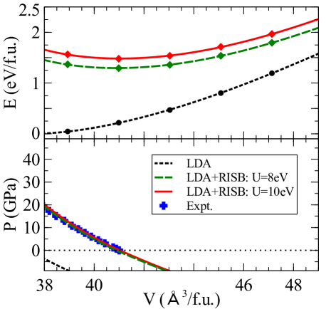
Figure 1: (Color online) Zero temperature LDA and LDA+RISB total energies (upper panel) and corresponding pressure-volume phase diagrams compared with the room-temperature experiments of Ref. Idiri et al., 2004 (lower panel).

In the upper panel of Fig. 1 are shown the LDA and LDA+RISB total energies $E(V)$ obtained at zero temperature for $U=8\,eV$ and $U=10\,eV$. The corresponding pressure (P-V) curves, obtained from $P(V)=-dE/dV$, are shown in the lower panel in comparison with the experimental data of Ref. Idiri et al., 2004 (which were obtained at room temperature). As anticipated in the main text, we observe that the P-V curve (and, in particular, the equilibrium volume) is essentially identical for $U=8\,eV$, as changing $U$ results in an energy shift that is essentially volume independent. The agreement with the experiment is remarkably good with both of the values of $U$ considered.

7.5 E.   Full matrix quasi-particle weights UO₂

For completeness, below we report the complete representation of the matrix of quasi-particle weights $Z=\mathcal{R}^{\dagger}\mathcal{R}$ of the U-$5f$ electrons in the basis [Eq. 16] of the main text:

$$Z_{\Gamma_{8}}=\begin{bmatrix}|\Gamma_{8}^{(1)},5/2,+\rangle&|\Gamma_{8}^{(2)},7/2,-\rangle&|\Gamma_{8}^{(1)},5/2,-\rangle&|\Gamma_{8}^{(2)},7/2,+\rangle&|\Gamma_{8}^{(2)},5/2,+\rangle&|\Gamma_{8}^{(1)},7/2,-\rangle&|\Gamma_{8}^{(2)},5/2,-\rangle&|\Gamma_{8}^{(1)},7/2,+\rangle\\ \hline\cr 0.1079&0.2952&0&0&0&0&0&0\\ 0.2952&0.8073&0&0&0&0&0&0\\ 0&0&0.1079&0.2952&0&0&0&0\\ 0&0&0.2952&0.8073&0&0&0&0\\ 0&0&0&0&0.1079&0.2952&0&0\\ 0&0&0&0&0.2952&0.8073&0&0\\ 0&0&0&0&0&0&0.1079&0.2952\\ 0&0&0&0&0&0&0.2952&0.8073\end{bmatrix}$$

$$Z_{\Gamma_{7}}=\begin{bmatrix}|\Gamma_{7},5/2,+\rangle&|\Gamma_{7},7/2,-\rangle&|\Gamma_{7},5/2,-\rangle&|\Gamma_{7},7/2,+\rangle\\ \hline\cr 0.9244&0.0125&0&0\\ 0.0125&0.9489&0&0\\ 0&0&0.9244&0.0125\\ 0&0&0.0125&0.9489\end{bmatrix}\;\;\;Z_{\Gamma_{6}}=\begin{bmatrix}|\Gamma_{6},7/2,+\rangle&|\Gamma_{6},7/2,-\rangle\\ \hline\cr 0.9515&0\\ 0&0.9515\end{bmatrix}$$

Because of the Schur lemma, the states belonging to inequivalent representations are not coupled by the self energy (and, consequently, by $Z$). Note that, as discussed in the main text, the off-diagonal matrix elements of $Z$ coupling $5/2$ and $7/2$ states are not negligible.

7.6 F.   Single-particle density matrix UO₂

Below we report the complete representation of the single-particle density matrix $\rho_{\alpha\beta}=\langle c^{\dagger}_{\alpha}c^{\phantom{\dagger}}_{\beta}\rangle$ of the U-$5f$ electrons in the basis [Eq. 16] of the main text:

$$\rho_{\Gamma_{8}}=\begin{bmatrix}|\Gamma_{8}^{(1)},5/2,+\rangle\!&\!|\Gamma_{8}^{(2)},7/2,-\rangle\!&\!|\Gamma_{8}^{(1)},5/2,-\rangle\!&\!|\Gamma_{8}^{(2)},7/2,+\rangle\!&\!|\Gamma_{8}^{(2)},5/2,+\rangle\!&\!|\Gamma_{8}^{(1)},7/2,-\rangle\!&\!|\Gamma_{8}^{(2)},5/2,-\rangle\!&\!|\Gamma_{8}^{(1)},7/2,+\rangle\\ \hline\cr 0.468\!\!&\!\!0.018\!-\!0.059i&0&0&0&0&0&0\\ 0.018\!+\!0.059i\!\!&\!\!0.026&0&0&0&0&0&0\\ 0&0&0.4678\!\!&\!\!0.018\!-\!0.059i&0&0&0&0\\ 0&0&0.018\!+\!0.059i\!\!&\!\!0.026&0&0&0&0\\ 0&0&0&0&0.468\!\!&\!\!0.018\!-\!0.059i&0&0\\ 0&0&0&0&0.018\!+\!0.059i\!\!&\!\!0.026&0&0\\ 0&0&0&0&0&0&0.468\!\!&\!\!0.018\!-\!0.059i\\ 0&0&0&0&0&0&0.018\!+\!0.059i\!\!&\!\!0.026\end{bmatrix}$$

$$\rho_{\Gamma_{7}}=\begin{bmatrix}|\Gamma_{7},5/2,+\rangle&|\Gamma_{7},7/2,-\rangle&|\Gamma_{7},5/2,-\rangle&|\Gamma_{7},7/2,+\rangle\\ \hline\cr 0.067&0.007\!-\!0.001i&0&0\\ 0.007\!+\!0.001i&0.035&0&0\\ 0&0&0.067&0.007\!-\!0.001i\\ 0&0&0.007\!+\!0.001i&0.035\end{bmatrix}\;\;\;\rho_{\Gamma_{6}}=\begin{bmatrix}|\Gamma_{6},7/2,+\rangle&|\Gamma_{6},7/2,-\rangle\\ \hline\cr 0.020&0\\ 0&0.020\end{bmatrix}$$

Note that, because of the Shur lemma, $\rho$ has the same block structure of the matrix $Z$.

We point out that the numbers reported in Table I of the main text correspond to the diagonal elements of the matrix $\rho$ in the basis that diagonalizes $Z$ (that is not the same basis that diagonalizes $\rho$).

7.7 G.   Many-body configuration probabilities UO₂

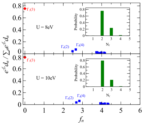
Figure 2: (Color online) Configuration probabilities of the eigenstates of the local reduced density matrix $\hat{\rho}_{f}\equiv e^{-\hat{F}}/\mathrm{Tr}[e^{-\hat{F}}]$ of the $5f$ electrons shown as a function of the eigenvalues $f_{n}$ of $\hat{F}$ at $V_{\text{eq}}\simeq 41\,\AA/\text{f.u.}$ for 2 different values of $U$. The labels of the irreducible representations and their respective degeneracies are expressed using the Koster notation. The corresponding occupation probabilities $\mathrm{Tr}\big{[}\hat{\rho}_{f}\hat{N}_{f}\big{]}$ are shown in the insets.

In Fig. 2 are shown the eigenvalues of the local reduced density matrix $\hat{\rho}_{f}$ of the U-$5f$ electrons — which is formally obtained from the full many-body density matrix of the system by tracing out all of the degrees of freedom with the exception of the $5f$ local many-body configurations of the U atoms. As in Ref. Lanatà et al., 2015, $\hat{\rho}_{f}$ is represented as $e^{-\hat{F}}/\mathrm{Tr}[e^{-\hat{F}}]$, and the corresponding eigenvalues (configuration probabilities) are displayed as a function of the corresponding eigenvalues $f_{n}$ of $\hat{F}$ (entanglement spectrum). In the insets is shown also the histogram of occupation probabilities:

$$P_{N}\equiv\mathrm{Tr}\big{[}\hat{\rho}_{f}\hat{N}_{f}\big{]}\,,$$ (138)

where $\hat{N}_{f}$ is the number operator of the U-$5f$ states. The so obtained histogram is very similar for the 2 values of interaction strength $U$ considered.

Note that, because of the crystal field splittings, the eigenstates of $\hat{\rho}_{f}$ generate irreducible representations of the double $O$ point group of the U atom, whose transformation properties are represented in Fig. 2 using the Koster notation.

Consistently with previous theoretical Santini et al. (2009); Zhou and Ozoliņš (2011); Suzuki et al. (2013) and experimental Amoretti et al. (1989); Nakotte et al. (2010) studies, we find that the most probable local configuration is a $f^{2}$ $\Gamma_{5}$ triplet, which has probability $P_{\Gamma_{5}}^{f^{2}}\sim 0.8$ according to our calculations. We point out that the $f^{2}$ many-body space contains $12$ $\Gamma_{5}$ representations. Consequently, the above-mentioned most probable eigenspace of $\hat{\rho}_{f}$, that we name $V_{\Gamma_{5}}^{f^{2}}$, can not be determined exclusively by its symmetry properties, but has to be calculated. For completeness, here we report the explicit representation of the states spanning $V_{\Gamma_{5}}^{f^{2}}$ in the Fock basis generated by the single-particle states defined in Eq. 16 of the main text:

$$\{|\alpha\rangle\,|\,\alpha=1,..,14\}=$$

$$\;\big{\{}|\Gamma_{8}^{(1)},5/2,+\rangle,|\Gamma_{8}^{(2)},7/2,-\rangle,|\Gamma_{8}^{(1)},5/2,-\rangle,|\Gamma_{8}^{(2)},7/2,+\rangle,|\Gamma_{8}^{(2)},5/2,+\rangle,|\Gamma_{8}^{(1)},7/2,-\rangle,|\Gamma_{8}^{(2)},5/2,-\rangle,|\Gamma_{8}^{(1)},7/2,+\rangle,$$

$$\;|\Gamma_{7},5/2,+\rangle,|\Gamma_{7},7/2,-\rangle,|\Gamma_{7},5/2,-\rangle,|\Gamma_{7},7/2,+\rangle,|\Gamma_{6},7/2,+\rangle,|\Gamma_{6},7/2,-\rangle\big{\}}\,.$$ (139)

Within the following notation:

$$|\Gamma_{5},n\rangle=\sum_{\alpha=2}^{14}\sum_{\beta=1}^{\alpha-1}M_{\alpha\beta}^{n}\,c^{\dagger}_{\alpha}c^{\dagger}_{\beta}\,|0\rangle\;,\qquad\quad n=1,2,3\,,$$ (140)

the states $|\Gamma_{5},n\rangle$ are specified by the following coefficients:

$$M^{1}_{21} = -0.004+0.042i$$

$$M^{1}_{3\beta} = (0,0)$$

$$M^{1}_{4\beta} = (0,0,0.005-0.01i)$$

$$M^{1}_{5\beta} = (-0.154+0.25i,0.03-0.049i,-0.074+0.808i,0.008-0.085i)$$

$$M^{1}_{6\beta} = (0.012-0.019i,-0.004+0.006i,0.012-0.134i,-0.002+0.021i,-0.005+0.01i)$$

$$M^{1}_{7\beta} = (0.097-0.195j,-0.01+0.021i,-0.154+0.25i,0.03-0.049i,0,0)$$

$$M^{1}_{8\beta} = (-0.016+0.032i,0.003-0.005i,0.012-0.019i,-0.004+0.006i,0,0,0.004-0.042i)$$

$$M^{1}_{9\beta} = (-0.016+0.171i,0.007-0.073i,0,0,0.038-0.061i,-0.016+0.026i,0.012-0.024i,$$

$$-0.005+0.01i)$$

$$M^{1}_{10\beta} = (0.005-0.06i,-0.002+0.022i,0,0,-0.013+0.021i,0.005-0.008i,-0.004+0.008i,$$

$$0.002-0.003i,0)$$

$$M^{1}_{11\beta} = (0,0,0.021-0.041i,-0.009+0.018i,-0.009+0.099i,0.004-0.042i,0.038-0.061i,$$

$$-0.016+0.026i,0,0)$$

$$M^{1}_{12\beta} = (0,0,-0.007+0.014i,0.003-0.005i,0.003-0.035i,-0.001+0.013i,-0.013+0.021i,$$

$$0.005-0.008i,0,0,0)$$

$$M^{1}_{13\beta} = (0.004-0.008i,0.001-0.003i,0.013-0.021i,0.004-0.006i,0,0,0.005-0.06i,0.002-0.018i,$$

$$-0.007+0.014i,0.004-0.007i,0.011-0.017i,-0.006+0.009i)$$

$$M^{1}_{14\beta} = (-0.013+0.021i,-0.004+0.006i,0.003-0.034i,0.001-0.01i,0.007-0.014i,0.002-0.004i,$$ (141)

$$0,0,-0.011+0.017i,0.006-0.009i,-0.005+0.056i,0.003-0.030i,0)$$

$$M^{2}_{21} = -0.015-0.007j$$

$$M^{2}_{3\beta} = (0,0)$$

$$M^{2}_{4\beta} = (0,0,-0.030-0.034i)$$

$$M^{2}_{5\beta} = (0.069+0.083i,-0.013-0.016i,-0.279-0.14i,0.029+0.015i)$$

$$M^{2}_{6\beta} = (-0.005-0.006i,0.002+0.002i,0.046+0.023i,-0.007-0.004i,0.03+0.034i)$$

$$M^{2}_{7\beta} = (-0.574-0.655i,0.061+0.069i,0.069+0.083i,-0.013-0.016i,0,0)$$

$$M^{2}_{8\beta} = (0.095+0.109i,-0.015-0.017i,-0.005-0.006i,0.002+0.002i,0,0,0.015+0.007i)$$

$$M^{2}_{9\beta} = (-0.059-0.03i,0.025+0.013i,0,0,-0.017-0.02i,0.007+0.009i,-0.07-0.08i,0.03+0.034i)$$

$$M^{2}_{10\beta} = (0.021+0.01i,-0.008-0.004i,0,0,0.006+0.007i,-0.002-0.003i,0.025+0.028i,-0.009-0.01i,0)$$

$$M^{2}_{11\beta} = (0,0,-0.122-0.139i,0.052+0.059i,-0.034-0.017i,0.014+0.007i,-0.017-0.02i,0.007+0.009i,0,0)$$

$$M^{2}_{12\beta} = (0,0,0.043+0.048i,-0.016-0.018i,0.012+0.006i,-0.004-0.002i,0.006+0.007i,-0.002-0.003i,0,0,0)$$

$$M^{2}_{13\beta} = (-0.024-0.028i,-0.007-0.008i,-0.006-0.007i,-0.002-0.002i,0,0,0.021+0.01i,0.006+0.003i,$$

$$0.04+0.046i,-0.021-0.024i,-0.005-0.006i,0.003+0.003i)$$

$$M^{2}_{14\beta} = (0.006+0.007i,0.002+0.002i,0.012+0.006i,0.004+0.002i,-0.042-0.048i,-0.013-0.015i,0,0,$$ (142)

$$0.005+0.006i,-0.003-0.003i,-0.019-0.01i,0.01+0.005i,0)$$

$$M^{3}_{21} = 0.018+0.001i$$

$$M^{3}_{3\beta} = (0,0)$$

$$M^{3}_{4\beta} = (0,0,-0.013-0.006i)$$

$$M^{3}_{5\beta} = (-0.513-0.280i,0.101+0.055i,0.35+0.011i,-0.037-0.001i)$$

$$M^{3}_{6\beta} = (0.039+0.021i,-0.013-0.007i,-0.058-0.002i,0.009+0.000i,0.013+0.006i)$$

$$M^{3}_{7\beta} = (-0.244-0.117i,0.026+0.012i,-0.513-0.280i,0.101+0.055i,0,0)$$

$$M^{3}_{8\beta} = (0.04+0.019i,-0.006-0.003i,0.039+0.021i,-0.013-0.007i,0,0,-0.018-0.001i)$$

$$M^{3}_{9\beta} = (0.074+0.002i,-0.031-0.001i,0,0,0.126+0.069i,-0.053-0.029i,-0.03-0.014i,0.013+0.006i)$$

$$M^{3}_{10\beta} = (-0.026-0.001i,0.01,0,0,-0.044-0.024i,0.016+0.009i,0.01+0.005i,-0.004-0.002i,0)$$

$$M^{3}_{11\beta} = (0,0,-0.052-0.025i,0.022+0.010i,0.043+0.001i,-0.018-0.001i,0.126+0.069i,-0.053-0.029i,0,0)$$

$$M^{3}_{12\beta} = (0,0,0.018+0.009i,-0.007-0.003i,-0.015,0.006,-0.044-0.024i,0.016+0.009i,0,0,0)$$

$$M^{3}_{13\beta} = (-0.010-0.005i,-0.003-0.001i,0.044+0.024i,0.013+0.007i,0,0,-0.026-0.001i,-0.008,$$

$$0.017+0.008i,-0.009-0.004i,0.036+0.02i,-0.019-0.01i)$$

$$M^{3}_{14\beta} = (-0.044-0.024i,-0.013-0.007i,-0.015,-0.004,-0.018-0.009i,-0.005-0.003i,0,0,$$ (143)

$$-0.036-0.02i,0.019+0.01i,0.024+0.001i,-0.013,0)\,.$$

We observe that the remaining probability weight, which is not negligible, is distributed mostly among $f^{3}$ configurations, whose Koster symbols are displayed explicitly in Fig. 2 for the most probable multiplets.

References

Koga et al. (2004)A. Koga, N. Kawakami,
T. M. Rice, and M. Sigrist, Phys. Rev. Lett. 92, 216402 (2004).
Anisimov et al. (2002)V. Anisimov, I. Nekrasov,
D. Kondakov, T. M. Rice, and M. Sigrist, Eur. Phys. J. B 25, 191 (2002).
de’ Medici et al. (2009)L. de’
Medici, S. R. Hassan,
M. Capone, and X. Dai, Phys. Rev. Lett. 102, 126401 (2009).
Lanatà et al. (2013)N. Lanatà, H. U. R. Strand, G. Giovannetti,
B. Hellsing, L. de’ Medici, and M. Capone, Phys. Rev. B 87, 045122 (2013).
Dobrosavljević et al. (2012)V. Dobrosavljević, N. Trivedi, and J. M. Valles Jr., Conductor Insulator Quantum Phase Transitions (Oxford University Press, UK, 2012).
Marianetti et al. (2004)C. A. Marianetti, G. Kotliar,
and G. Ceder, Nature Materials 3, 627 (2004).
Camjayi et al. (2008)A. Camjayi, K. Haule,
V. Dobrosavljević, and G. Kotliar, Nature Phys. 4, 932 (2008).
Kotliar and Ruckenstein (1986)G. Kotliar and A. E. Ruckenstein, Phys. Rev. Lett. 57, 1362 (1986).
Lechermann et al. (2007)F. Lechermann, A. Georges,
G. Kotliar, and O. Parcollet, Phys. Rev. B 76, 155102 (2007).
Li et al. (1989)T. Li, P. Wölfle, and P. J. Hirschfeld, Phys. Rev. B 40, 6817 (1989).
Bhatia (2007)R. Bhatia, Positive Definite
Matrices (Princeton University Press, Princeton
and Oxford, 2007).
Zhou and Ozoliņš (2011)F. Zhou and V. Ozoliņš, Phys. Rev. B 83, 085106
(2011).
Suzuki et al. (2013)M.-T. Suzuki, N. Magnani, and P. M. Oppeneer, Phys. Rev. B 88, 195146 (2013).
Amoretti et al. (1989)G. Amoretti, A. Blaise,
R. Caciuffo, J. M. Fournier, M. T. Hutchings, R. Osborn, and A. D. Taylor, Phys. Rev. B 40, 1856 (1989).
Nakotte et al. (2010)H. Nakotte, R. Rajaram,
S. Kern, R. J. McQueeney, G. H. Lander, and R. A. Robinson, J. Phys.: Conf. Ser. 251, 012002 (2010).
Schönhammer (1990)K. Schönhammer, Phys. Rev. B 42, 2591
(1990).
Georges et al. (1996)A. Georges, G. Kotliar,
W. Krauth, and M. J. Rozenberg, Rev. Mod. Phys. 68, 13 (1996).
Anisimov et al. (1997b)V. I. Anisimov, A. I. Oteryaev, M. A. Korotin, A. O. Anokhin, and G. Kotliar, J.
Phys. Condens. Matter 9, 7359 (1997b).
Lichtenstein and Katsnelson (2000)A. I. Lichtenstein and M. I. Katsnelson, Phys. Rev. B 62, R9283
(2000).
Note (1)The interplay between SOC and CFS can generate multiple
equivalent representations of the point symmetry group in the local single
particle space, so that is not made automatically diagonal
by selection rules Wigner (1959).
Wigner (1959)E. P. Wigner, Group theory and its
application to the quantum mechanics of atomic spectra (Academic Press, 1959).
Geng et al. (2007)H. Y. Geng, Y. Chen, Y. Kaneta, and M. Kinoshita, Phys. Rev. B 75, 054111 (2007).
Wang et al. (2013)B.-T. Wang, P. Zhang,
R. Lizárraga, I. Di Marco, and O. Eriksson, Phys. Rev. B 88, 104107 (2013).
Laskowski et al. (2004)R. Laskowski, G. K. H. Madsen, P. Blaha, and K. Schwarz, Phys. Rev. B 69, 140408 (2004).
Kudin et al. (2002)K. N. Kudin, G. E. Scuseria,
and R. L. Martin, Phys. Rev. Lett. 89, 266402 (2002).
Prodan et al. (2006)I. D. Prodan, G. E. Scuseria, and R. L. Martin, Phys.
Rev. B 73, 045104
(2006).
Frazer et al. (1965)B. C. Frazer, G. Shirane,
D. E. Cox, and C. E. Olsen, Phys. Rev. 140, A1448 (1965).
Blaha et al. (2001)P. Blaha, K. Schwarz,
G. Madsen, D. Kvasnicka, and J. Luitz, an augmented plane wave plus
local orbitals program for calculating crystal properties. University of
Technology, Vienna (2001).
Idiri et al. (2004)M. Idiri, T. Le Bihan,
S. Heathman, and J. Rebizant, Phys. Rev. B 70, 014113 (2004).
Note (2)Smaller values of have not been considered because,
within our LDA+RISB functional, the system would result metallic for
(which is the value of the
screened Hubbard interaction parameter previously computed in Ref. Amadon et al. (2014)) and, at the same time, the agreement with the experimental P-V
curve would worsen.
Amadon et al. (2014)B. Amadon, T. Applencourt,
and F. Bruneval, Phys. Rev. B 89, 125110 (2014).
Dresselhaus et al. (2007)M. S. Dresselhaus, G. Dresselhaus, and A. Jorio, Group Theory, Application
to the Physics of Condensed Matter (Springer, 2007).
Note (3)In this work we adopted the so called Koster
notation.
Tobin et al. (2015)J. G. Tobin, S.-W. Yu,
R. Qiao, W. L. Yang, C. H. Booth, D. K. Shuh, A. M. Duffin, D. Sokaras, D. Nordlund, and T.-C. Weng, Phys. Rev. B 92, 045130 (2015).
Moore et al. (2006)K. T. Moore, G. van der Laan,
R. G. Haire, M. A. Wall, and A. J. Schwartz, Phys. Rev. B 73, 033109 (2006).
Prodan et al. (2007)I. D. Prodan, G. E. Scuseria, and R. L. Martin, Phys.
Rev. B 76, 033101
(2007).
Booth et al. (2016)C. H. Booth, S. A. Medling,
J. G. Tobin, R. E. Baumbach, E. D. Bauer, D. Sokaras, D. Nordlund, and T.-C. Weng, Phys. Rev. B 94, 045121 (2016).
Puschnig et al. (2009)P. Puschnig, S. Berkebile,
A. Fleming, G. Koller, K. Emtsev, T. Seyller, J. Riley, C. Ambrosch-Draxl, F. Netzer, and M. Ramsey, Science 326, 702 (2009).
Ziroff et al. (2010)J. Ziroff, F. Forster,
A. Schöll, P. Puschnig, and F. Reinert, Phys. Rev. Lett. 104, 233004 (2010).
Baer and Schoenes (1980)Y. Baer and J. Schoenes, Solid State Commun. 33, 885 (1980).
Tobin and Yu (2011)J. G. Tobin and S.-W. Yu, Phys. Rev. Lett. 107, 167406 (2011).
Santini et al. (2009)P. Santini, S. Carretta,
G. Amoretti, R. Caciuffo, N. Magnani, and G. H. Lander, Rev. Mod. Phys. 81, 807 (2009).

References

Lanatà et al. (2015)N. Lanatà, Y. Yao,
C.-Z. Wang, K.-M. Ho, and G. Kotliar, Phys. Rev. X 5, 011008 (2015).
Lechermann et al. (2007)F. Lechermann, A. Georges,
G. Kotliar, and O. Parcollet, Phys. Rev. B 76, 155102 (2007).