Variants of Kinetically Modified Non-Minimal Higgs Inflation in Supergravity

Abstract

We consider models of chaotic inflation driven by the real parts of a conjugate pair of Higgs superfields involved in the spontaneous breaking of a grand unification symmetry at a scale assuming its Supersymmetric (SUSY) value. Employing Kähler potentials with a prominent shift-symmetric part proportional to $c_{-}$ and a tiny violation, proportional to $c_{+}$, included in a logarithm we show that the inflationary observables provide an excellent match to the recent Planck and Bicep2/Keck Array results setting, e.g., $6.4\cdot 10^{-3}\lesssim r_{\pm}=c_{+}/c_{-}\lesssim 1/N$ where $N=2$ or $3$ is the prefactor of the logarithm. Deviations of these prefactors from their integer values above are also explored and a region where hilltop inflation occurs is localized. Moreover, we analyze two distinct possible stabilization mechanisms for the non-inflaton accompanying superfield, one tied to higher order terms and one with just quadratic terms within the argument of a logarithm with positive prefactor $N_{S}<6$. In all cases, inflation can be attained for subplanckian inflaton values with the corresponding effective theories retaining the perturbative unitarity up to the Planck scale.

Keywords: Cosmology of Theories Beyond the Standard Model, Supergravity Models;
PACS codes: 98.80.Cq, 11.30.Qc, 12.60.Jv, 04.65.+e

Published in J. Cosmol. Astropart. Phys. 10, 037, no. 10, (2016)

1 Introduction

In a series of recent papers [1, 2, 3] we established a novel type of non-minimal inflation (nMI) called kinetically modified. This term is coined in Ref. [1] due to the fact that, in the non-SUSY set-up, this inflationary model, based on the $\phi^{p}$ power-law potential, employs not only a suitably selected coupling to gravity $f_{\cal R}=1+c_{\cal R}\phi^{p/2}$ but also a kinetic mixing of the form $f_{\rm K}=c_{\rm K}f_{\cal R}^{m}$. The merits of this construction compared to the original (and more economical) model [4, 5, 6, 7] of nMI (defined for $f_{\rm K}=1$) are basically two:

• The observational outputs depend on the ratio $r_{{\cal R}K}=c_{\cal R}/c_{\rm K}^{p/4}$ and can be done excellently consistent with the recent Planck [8] and Bicep2/Keck Array [9, 10] results;

• The resulting theory respects the perturbative unitarity [11, 12] up to the Planck scale for any $p$ and $m$ and $r_{{\cal R}K}\leq 1$.

In the SUSY – which means Supergravity (SUGRA) – framework the two ingredients necessary to achieve this kind of nMI, i.e., the non-minimal kinetic mixing and coupling to gravity, originate from the same function, the Kähler potential, and the set-up becomes much more attractive. Particularly intriguing is the version of these models, called henceforth non-minimal Higgs inflation (nMHI), in which the inflaton, at the end of its inflationary evolution, can also play the role of a Higgs field [4, 13, 14, 15, 2, 3]. Actually in Ref. [3] we present a class of Kähler potentials which cooperate with the simplest superpotential [16] widely used for implementing spontaneously breaking of a Grand Unified Theory (GUT) gauge group $G_{\rm GUT}$. In this framework, the non-minimal kinetic mixing and gravitational coupling of the inflaton can be elegantly realized introducing an approximate shift symmetry [17, 18, 2, 3] respected by the Kähler potential. As a consequence, the constants $c_{\rm K}$ and $c_{\cal R}$ introduced above can be interpreted as the coefficients of the principal shift-symmetric term ($c_{-}$) and its violation ($c_{+}$) while $r_{{\cal R}K}$ is now written as $r_{\pm}=c_{+}/c_{-}$ – obviously $p=4$ in this set-up.

Trying to highlight the most important issues of our suggestion in Ref. [3], we employ only integer coefficients of the logarithms appearing in the Kähler potentials. However, as we show in the particular case of Ref. [2] – see also Refs. [20, 19, 21] – the variation of the prefactors of the logarithms in the Kähler potentials can have a pronounced impact on the inflationary observables. Consequently, it would be interesting to investigate which inflationary solutions can be obtained in this variance of the simplified initial set-up. Moreover, we have here the opportunity to test our proposal against the latest obervational data on the gravitational waves [10]. We also check the wide applicability of a novel stabilization mechanism for the non-inflaton accompanied field, recently proposed in the context of the Starobinsky-type inflation in Ref. [22]. In addition to the results similar to those found in Refs. [2, 3], we here establish a sizable region of the parameter space where nMHI of hilltop type [23] is achieved.

The super- and Kähler potentials of our models are presented in Sec. 2. In Sec. 3 we describe our inflationary set-up, whereas in Sec. 4 we derive the inflationary observables and confront them with observations. Our conclusions are summarized in Sec. 5. Throughout the text, we use units where the reduced Planck scale $m_{\rm P}=2.433\cdot 10^{18}~{}{\mbox{\rm GeV}}$ is set to be unity, the subscript of type $,\chi$ denotes derivation with respect to (w.r.t) the field $\chi$ – e.g., $F_{,\chi\chi}=\partial^{2}F/\partial\chi^{2}$ – and charge conjugation is denoted by a star (^∗).

2 Supergravity Set-up

The Einstein frame (EF) action within SUGRA for the complex scalar fields $z^{\alpha}=S,\Phi,\bar{\Phi}$ – denoted by the same superfield symbol – can be written as [24]

$${\sf S}=\int d^{4}x\sqrt{-\widehat{\mathfrak{g}}}\left(-\frac{1}{2}\widehat{\mathcal{R}}+K_{{\alpha}{\bar{\beta}}}\widehat{g}^{\mu\nu}D_{\mu}z^{\alpha}D_{\nu}z^{*{\bar{\beta}}}-\widehat{V}\right)$$ (1a)

where summation is taken over $$z^{\alpha} D_{\mu} K K_{{\alpha}{\bar{\beta}}}=K_{,z^{\alpha}z^{*{\bar{\beta}}}} K^{{\alpha}{\bar{\beta}}}K_{{\bar{\beta}}\gamma}=\delta^{\alpha}_{\gamma} \widehat{V}$$; is the gauge covariant derivative, is the Kähler potential, with and . Also is the EF SUGRA potential which can be found via the formula

$$\widehat{V}=e^{K}\left(K^{{\alpha}{\bar{\beta}}}D_{\alpha}WD^{*}_{\bar{\beta}}W^{*}-3{|W|^{2}}\right)+\frac{g^{2}}{2}\mbox{$\sum_{a}$}{\rm D}_{a}{\rm D}_{a},$$ (1b)

where $D_{\alpha}W=W_{,z^{\alpha}}+K_{,z^{\alpha}}W$, with $W$ being the superpotential, ${\rm D}_{a}=z_{\alpha}\left(T_{a}\right)^{\alpha}_{\beta}K^{\beta}$, $g$ is the unified gauge coupling constant and the summation is applied over the generators $T_{a}$ of $G_{\rm GUT}$. Just for definiteness we restrict ourselves to $G_{\rm GUT}=G_{\rm SM}\times U(1)_{B-L}$ [2, 3], gauge group which consists the simplest GUT beyond the Minimal SUSY Standard Model (MSSM) based on the gauge group ${G_{\rm SM}}=SU(3)_{\rm C}\times SU(2)_{\rm L}\times U(1)_{Y}$ – here ${G_{\rm SM}}=SU(3)_{\rm c}\times SU(2)_{\rm L}\times U(1)_{Y}$ is the gauge group of the standard model and $B$ and $L$ denote the baryon and lepton number, respectively.

As shown in Eq. (1b), the derivation of $\widehat{V}$ requires the specification of $W$ and $K$ presented in Secs. 2.1 and 2.2 respectively. In Sec. 2.3 we derive the SUSY vacuum.

2.1 Superpotential

We focus on the simplest $W$ which can be used to implement the Higgs mechanism in a SUSY framework. This is

$$W=\lambda S\left(\bar{\Phi}\Phi-M^{2}/4\right)$$ (2)

and is uniquely determined, at renormalizable level, by a convenient [16] continuous $R$ symmetry. Here $\lambda$ and $M$ are two constants which can both be taken positive; $S$ is a left-handed superfield, singlet under $G_{\rm GUT}$; $\Phi$ and $\bar{\Phi}$ is a pair of left-handed superfields which carry $B-L$ charges $1$ and $-1$ respectively and lead to a breaking of $G_{\rm GUT}$ down to $G_{\rm SM}$ by their vacuum expectation values (v.e.vs).

$W$ in Eq. (2), combined with a canonical [25] or quasi-canonical $K$ [27, 26], can support F-term hybrid inflation driven by $S$ with the $\bar{\Phi}-\Phi$ system being stabilized at zero. This type of inflation is terminated by a destabilization of the the $\bar{\Phi}-\Phi$ system which is led to the SUSY vacuum during the so-called waterfall regime. Therefore, a GUT phase transition takes place at the end of inflation. Topological defects (cosmic strings in the case of $G_{\rm GUT}$ considered here) are, thus, copiously formed if they are predicted by the symmetry breaking. In our proposal we interchange the roles of the inflaton and the waterfall fields attaining inflation driven by $\bar{\Phi}-\Phi$ system and setting $S$ stabilized at the origin during and after nMHI. As a consequence $G_{\rm GUT}$ is already spontaneously broken during nMHI through the non-zero values acquired by $\bar{\Phi}-\Phi$ and so, nMHI is not followed by the production of cosmic defects. To implement such an inflationary scenario we have to adopt logarithmic $K$’s presented below.

2.2 Kähler   Potentials

The implementation of the standard (large-field) nMHI [24, 14] – for small-field nMHI see Ref. [15] – requires the adoption of a logarithmic $K$ including an holomorphic term $c_{\cal R}\Phi\bar{\Phi}$ in its argument together with the usual kinetic terms. The resulting model has three shortcomings: (i) For $c_{\cal R}\gg 1$, the perturbative unitarity is violated below $m_{\rm P}$ [11, 12]; (ii) The predicted $r$ lies marginally within the $1-\sigma$ region of Bicep2/Keck Array results [10]; (iii) Possible inclusion of higher order terms of the form $|S|^{2}\left(k_{S\Phi}|\Phi|^{2}+k_{S\bar{\Phi}}|\bar{\Phi}|^{2}\right)$ in $K$ generally violate [28] the D-flatness unless an ugly tuning is imposed with $k_{S\Phi}=k_{S\bar{\Phi}}$.

All the issues above can be overcome, as we show below, if we assume the existence of an approximate shift symmetry on the $K$’s along the lines of Ref. [2, 3] – the importance of the shift symmetry in taming the so-called $\eta$-problem of inflation in SUGRA is first recognized for gauge singlets in Ref. [17] and non-singlets in Ref. [18]. More specifically, to achieve kinetically modified nMHI we select purely or partially logarithmic $K$’s including the real functions

$$F_{\pm}=\left|\Phi\pm\bar{\Phi}^{*}\right|^{2}~{}~{}\mbox{and}~{}~{}F_{1S}=|S|^{2}-k_{S}{|S|^{4}}~{}~{}\mbox{or}~{}~{}F_{2S}=1+|S|^{2}/N_{S}\,,~{}~{}$$ (3)

where, as we show in Sec. 3.1, $F_{-}$ and $F_{+}$ are related to the canonical normalization of inflaton and the non-minimal inflaton-curvature coupling respectively. Also $F_{1S}$ or $F_{2S}$ provides typical kinetic terms for $S$, considering the next-to-minimal term in $F_{1S}$ for stability reasons [24]. In terms of the functions introduced in Eq. (3) we postulate the following form of $K$

$$K_{1}=-{N_{1}}\ln\left(1+c_{+}F_{+}-\frac{1}{{N_{1}}}(1+c_{+}F_{+})^{m}c_{-}F_{-}-\frac{1}{{N_{1}}}F_{1S}+k_{\Phi}F_{-}^{2}+\frac{1}{{N_{1}}}k_{S-}F_{-}{|S|^{2}}\right)\,.~{}~{}~{}~{}~{}$$ (4a)

Here all the allowed terms up to fourth order are considered for $$c_{+}=0 c_{+} 1+c_{+}F_{+} c_{-}(1+c_{+}F_{+})^{m} F_{+}^{m} F_{+}^{m}|S|^{2}/3 F_{-} K=K_{2}$$. Switching on generates a violation of an enhanced symmetry – see below – and gives rise to the scenario of kinetically modified nMHI as defined in Sec. 1. Namely, the term plays the role of the non-minimal gravitational coupling whereas the factor dominates the nonminimal kinetic mixing. Other allowed terms such as or are neglected for simplicity or we have to assume that their coefficients are negligibly small. Identical results can be achieved if we place the first term outside the argument of the logarithm selecting with

$$K_{2}=-N_{2}\ln\left(1+c_{+}F_{+}-F_{1S}/{N_{2}}\right)+(1+c_{+}F_{+})^{m-1}c_{-}F_{-}\,.$$ (4b)

If we place $$F_{1S} K K$$ outside the argument of the logarithm in the two ’s above, we can obtain two other ’s which lead to similar results. Namely,

$$K_{3} = -N_{3}\ln\left(1+c_{+}F_{+}-(1+c_{+}F_{+})^{m}c_{-}F_{-}/N_{3}\right)+F_{1S}\,,$$ (4c)

$$K_{4} = -N_{4}\ln(1+c_{+}F_{+})+(1+c_{+}F_{+})^{m-1}c_{-}F_{-}+F_{1S}\,.$$ (4d)

If we employ $$F_{2S} K K_{3} K_{4} F_{1S} N_{S}\ln F_{2S}$$, the available ’s which lead to the same outputs with the previous ones have the form of and replacing with , i.e.,

$$K_{5} = -N_{5}\ln(1+c_{+}F_{+}-(1+c_{+}F_{+})^{m}c_{-}F_{-}/N_{5})+N_{S}\ln F_{2S}\,,~{}~{}~{}$$ (4e)

$$K_{6} = -N_{6}\ln\left(1+c_{+}F_{+}\right)+(1+c_{+}F_{+})^{m-1}c_{-}F_{-}\ +N_{S}\ln F_{2S}\,.$$ (4f)

Furthermore, allowing the term including $$F_{-} F_{2S} K$$ to share the same logarithmic argument with we can obtain a last expression of , i.e.,

$$K_{7}=-N_{7}\ln(1+c_{+}F_{+})+N_{S}\ln\left(F_{2S}+(1+c_{+}F_{+})^{m-1}c_{-}F_{-}/N_{S}\,\right)\,.$$ (4g)

The last three $K$’s are advantageous compared to the others since the stabilization of $S$ is achieved with just quadratic terms and so no higher order mix terms between $F_{\pm}$ and $S$ are necessary for consistency.

As we show in Sec. 3.1, the positivity of the kinetic energy of the inflaton sector requires $c_{+}<c_{-}$ and $N_{i}>0$ with $i=1,...,7$. For $r_{\pm}=c_{+}/c_{-}\ll 1$, our models are completely natural in the ’t Hooft sense because, in the limits $c_{+}\rightarrow 0$ and $\lambda\rightarrow 0$, $K_{i}$ with $i=1,...,4$ enjoy the following enhanced symmetries:

$$\Phi\rightarrow\ \Phi+C,\>\>\>\bar{\Phi}\rightarrow\ \bar{\Phi}+C^{*}\>\>\>\mbox{and}\>\>\>S\rightarrow\ e^{i\varphi}S,$$ (5a)

where $$C \varphi K_{i} i=5 6$$ [] is a complex [real] number. In the same limit, with and enjoy even more interesting enhanced symmetries:

$$\Phi\rightarrow\ \Phi+C,\>\>\>\bar{\Phi}\rightarrow\ \bar{\Phi}+C^{*}\>\>\>\mbox{and}\>\>\>\frac{S}{\sqrt{N_{S}}}\rightarrow\frac{aS/\sqrt{N_{S}}+b}{-b^{*}S/\sqrt{N_{S}}+a^{*}},$$ (5b)

with $$|a|^{2}+|b|^{2}=1 K=K_{5} K_{6} SU(2)_{S}/U(1) K_{7}$$. In other words, for or the theory exhibits a enhanced symmetry. Besides this symmetry, in the same limit, remains invariant (up to a Kähler transformation) under the continuous (non-holomorphic) transformations

$$\frac{S}{\sqrt{N_{S}}}\rightarrow\frac{aS/\sqrt{N_{S}}+b}{-b^{*}S/\sqrt{N_{S}}+a^{*}},\>\>\>\Phi\rightarrow\ \frac{\Phi}{-b^{*}S/\sqrt{N_{S}}+a^{*}}\>\>\>\mbox{and}\>\>\>\bar{\Phi}\rightarrow\ \frac{\bar{\Phi}}{-bS^{*}/\sqrt{N_{S}}+a}\cdot$$ (5c)

The kinetic terms, though, do not respect this symmetry and so, this is not valid at the level of the lagrangian.

In Sec. 4.3 we scan numerically the full parameter space of the models letting $m$ vary in the range $0\leq m\leq 10$ and allowing for a continuous variation of the $N_{i}$’s. On the other hand, we have to remark that for $m=0$ [$m=1$], $F_{-}$ and $F_{+}$ in $K_{1},K_{3}$ and $K_{5}$ [$K_{2},K_{4},K_{6}$ and $K_{7}$] are totally decoupled, i.e. no higher order term is needed. Given that the $m=0$ case with $N_{1}\leq 3$ or $N_{3}\leq 2$ is extensively analyzed in Ref. [2] we here focus mainly on $m=1$ with variable $N_{i}$’s – see Secs. 4.2.2 and 4.3. Moreover, keeping in mind that the most well-motivated $K$’s from the point of view of string theory are those with integer $N_{i}$’s – cf. Ref. [29] – we pay also special attention to the case with $N_{i}=3$ for $i=1,2$ or $N_{i}=2$ for $i=3,...,7$ – see Secs. 4.2.1 and 4.3.

2.3 SUSY Vacuum

To verify that the theories constructed lead to the breaking of $G_{B-L}$ down to $G_{\rm SM}$, we have to specify the SUSY limit $V_{\rm SUSY}$ of $\widehat{V}_{\rm HI}$ and minimize it. The potential $V_{\rm SUSY}$, which includes contributions from F- and D-terms, turns out to be

$$V_{\rm SUSY}=\widetilde{K}^{{\alpha}{\bar{\beta}}}W_{\alpha}W^{*}_{\bar{\beta}}+\frac{g^{2}}{2}\mbox{$\sum_{a}$}{\rm D}_{a}{\rm D}_{a}$$ (6a)

where $$\widetilde{K} K m_{\rm P}\rightarrow\infty$$ is the limit of ’s in Eqs. (4a) – (4g) for which is

$$\widetilde{K}=c_{-}F_{-}-Nc_{+}F_{+}+|S|^{2}\,.$$ (6b)

Upon substitution of $$\widetilde{K}$$ into Eq. (6a) we obtain

$$V_{\rm SUSY}=\lambda^{2}\left|\bar{\Phi}\Phi-\frac{M^{2}}{4}\right|^{2}+\frac{\lambda^{2}}{c_{-}(1-Nr_{\pm})}|S|^{2}\left(|\bar{\Phi}|^{2}+|\Phi|^{2}\right)+\frac{g^{2}}{2}c_{-}^{2}(1-Nr_{\pm})^{2}\left(|\bar{\Phi}|^{2}-|\Phi|^{2}\right)^{2}\,.$$ (6c)

From the last equation, we find that the SUSY vacuum lies along the D-flat direction $|\bar{\Phi}|=|\Phi|$ with

$$\langle{S}\rangle\simeq 0\>\>\>\mbox{and}\>\>\>|\langle{\Phi}\rangle|=|\langle{\bar{\Phi}}\rangle|=M/2,$$ (7)

from which we infer that $\langle{\Phi}\rangle$ and $\langle{\bar{\Phi}}\rangle$ break spontaneously $U(1)_{B-L}$, no only during nMHI but also at the vacuum of the theory. The contributions from the soft SUSY breaking terms can be safely neglected since the corresponding mass scale is much smaller than $M$. They may shift [30, 31], however, slightly $\langle{S}\rangle$ from zero in Eq. (7).

3 Inflationary Set-up

In this section, we outline the salient features of our inflationary scenario. In Sec. 3.1 we derive the tree-level inflationary potential and in Sec. 3.2 we consolidate its stability and its robustness against one-loop radiative corrections.

3.1 Tree-level Inflationary Potential

If we express $\Phi,\bar{\Phi}$ and $S$ according to the parametrization

$$\Phi=\frac{\phi e^{i{\theta}}}{\sqrt{2}}\cos{\theta_{\Phi}},~{}~{}\bar{\Phi}=\frac{\phi e^{i{\bar{\theta}}}}{\sqrt{2}}\sin{\theta_{\Phi}},~{}~{}\mbox{and}~{}~{}S=\frac{s+i\bar{s}}{\sqrt{2}}\,,$$ (8)

with $0\leq{\theta_{\Phi}}\leq\pi/2$, we can easily deduce from Eq. (1b) that a D-flat direction occurs at

$$\bar{s}=s={\theta}={\bar{\theta}}=0\>\>\>\mbox{and}\>\>\>{\theta_{\Phi}}={\pi/4}$$ (9)

along which the only surviving term in Eq. (1b) can be written universally as

$$\widehat{V}_{\rm HI}=e^{K}K^{SS^{*}}\,|W_{,S}|^{2}\,=\frac{\lambda^{2}(\phi^{2}-M^{2})^{2}}{16f_{\cal R}^{2(1+n)}}\,,~{}~{}~{}\mbox{where}~{}~{}~{}f_{\cal R}=1+c_{+}\phi^{2}$$ (10)

plays the role of a non-minimal coupling to Ricci scalar in the Jordan frame (JF). Indeed, if we perform a conformal transformation [24, 2] defining the frame function as

$${\Omega/N}=-\exp\left(-{K}/{N}\right),~{}~{}\mbox{where}~{}~{}N=N_{i}~{}~{}\mbox{for}~{}~{}K=K_{i}~{}~{}\mbox{with}~{}~{}i=1,...,7,$$ (11)

we can easily show that $f_{\cal R}=-\Omega/N$ along the path in Eq. (9). Since $M\ll 1$, we obtain $\langle{f_{\cal R}}\rangle\simeq 1$ at the SUSY vacuum in Eq. (7) and therefore the conventional Einstein gravity is recovered. For the derivation of Eq. (10), we also set

$$n=\begin{cases}{(N_{i}-1)/2}-1\\ {N_{2+j}/2}-1\end{cases}\mbox{and}~{}~{}K^{SS^{*}}=\begin{cases}f_{\cal R}\\ 1\end{cases}\mbox{for}~{}~{}K=\begin{cases}K_{i}&\mbox{with}\>\>i=1,2\\ K_{j+2}&\mbox{with}\>\>j=1,...,5.\end{cases}$$ (12)

Note that the exponent $n$ defined here has not to be confused with the one used in Ref. [1].

As deduced from Eq. (10) $\widehat{V}_{\rm HI}$ is independent from $c_{-}$ and $m$ which dominate, though, the canonical normalization of the inflaton. To specify it, we note that, for all $K$’s in Eqs. (4a) – (4g), $K_{{\alpha}{\bar{\beta}}}$ along the configuration in Eq. (9) takes the form

$$\left(K_{{\alpha}{\bar{\beta}}}\right)={\sf diag}\left(M_{K},K_{SS^{*}}\right)~{}~{}\mbox{with}~{}~{}M_{K}=\frac{1}{f_{\cal R}^{2}}\mbox{ $\left\lgroup\begin{matrix}\kappa&\bar{\kappa}\cr\bar{\kappa}&\kappa\end{matrix}\right\rgroup$},$$ (13)

where $\kappa=c_{-}f_{\cal R}^{2}-Nc_{+}$, $\bar{}\kappa={Nc_{+}^{2}\phi^{2}}$. Upon diagonalization of $M_{K}$ we find its eigenvalues which are

$$\kappa_{+}=\frac{c_{-}}{f_{\cal R}^{2}}\left(f_{\cal R}^{1+m}+Nr_{\pm}(c_{+}\phi^{2}-1)\right)\>\>\>\mbox{and}\>\>\>\kappa_{-}=\frac{c_{-}}{f_{\cal R}}\left(f_{\cal R}^{m}-{Nr_{\pm}}\right),$$ (14)

where the positivity of $\kappa_{-}$ is assured during and after nMHI for

$$r_{\pm}<f_{\cal R}^{m}/N~{}~{}\mbox{with}~{}~{}r_{\pm}=c_{+}/c_{-}\,.$$ (15)

Given that $f_{\cal R}^{m}>1$ for $m\geq 0$ and $\langle{f_{\cal R}}\rangle\simeq 1$, Eq. (15) implies that the maximal possible $r_{\pm}$ is $r_{\pm}^{\rm max}\simeq 1/N$. As shown numerically in Sec. 4.3, inflationary solutions with Eq. (15) fulfilled are attained only for $m\gtrsim-0.6$.

Inserting Eqs. (8) and (13) in the second term of the right-hand side (r.h.s) of Eq. (1a) we can, then, specify the EF canonically normalized fields, which are denoted by hat, as follows

$$K_{{\alpha}{\bar{\beta}}}\dot{z}^{\alpha}\dot{z}^{*{\bar{\beta}}} = {\kappa_{+}\over 2}\left(\dot{}\phi^{2}+{1\over 2}\phi^{2}\dot{\theta}^{2}_{+}\right)+{\kappa_{-}\over 2}\phi^{2}\left({1\over 2}\dot{\theta}^{2}_{-}+\dot{\theta}^{2}_{\Phi}\right)+\frac{1}{2}K_{SS^{*}}\left(\dot{s}^{2}+\dot{\bar{s}}^{2}\right)$$ (16a)

$$\simeq \frac{1}{2}\left(\dot{\widehat{}\phi}^{2}+\dot{\widehat{\theta}}_{+}^{2}+\dot{\widehat{\theta}}_{-}^{2}+\dot{\widehat{\theta}}_{\Phi}^{2}+\dot{\widehat{s}}^{2}+{\dot{\widehat{\bar{s}}}}^{~{}2}\right),$$

where $${\theta}_{\pm}=\left(\bar{\theta}\pm{\theta}\right)/\sqrt{2} K_{SS^{*}}=1/K^{SS^{*}} K^{SS^{*}} t J=\sqrt{\kappa_{+}}$$, with being given in Eq. (12) and the dot denotes derivation w.r.t the cosmic time, . Setting for later convenience , we can express the hatted fields in terms of the initial (unhatted) ones via the relations

$$\frac{d\widehat{\phi}}{d\phi}=J,\>\>\widehat{\theta}_{+}={J\over\sqrt{2}}\phi\theta_{+},\>\>\widehat{\theta}_{-}=\sqrt{\frac{\kappa_{-}}{2}}\phi\theta_{-},\>\>\widehat{\theta}_{\Phi}=\sqrt{\kappa_{-}}\phi\left(\theta_{\Phi}-\frac{\pi}{4}\right),(\widehat{s},\widehat{\bar{s}})=\sqrt{K_{SS^{*}}}(s,\bar{s})\,.$$ (16b)

As we show below the masses of the scalars besides $\widehat{\phi}$ during nMHI are heavy enough such that the dependence of the hatted fields on $\phi$ does not influence their dynamics – see also Ref. [14]. Note, in passing, that the spinors $\psi_{S}$ and $\psi_{\Phi\pm}$ associated with the superfields $S$ and $\Phi-\bar{\Phi}$ are normalized similarly, i.e., $\widehat{\psi}_{S}=\sqrt{K_{SS^{*}}}\psi_{S}$ and $\widehat{\psi}_{\Phi\pm}=\sqrt{\kappa_{\pm}}\psi_{\Phi\pm}$ with $\psi_{\Phi\pm}=(\psi_{\Phi}\pm\psi_{\bar{\Phi}})/\sqrt{2}$.

Fields	Eigen-	Masses Squared
	states		$K=K_{1}$	$K=K_{2}$	$K=K_{i+2}$	$K=K_{i+4}$	$K=K_{7}$
1 complex scalar	$\widehat{s},\widehat{\bar{s}}$	$\widehat{m}_{s}^{2}$	$6\left(2k_{S}f_{\cal R}-1/N_{i}\right)\widehat{H}_{\rm HI}^{2}$		$12k_{S}\widehat{H}_{\rm HI}^{2}$	$(6/N_{S})\widehat{H}_{\rm HI}^{2}$
2 real scalars	$\widehat{\theta}_{+}$	$\widehat{m}_{\theta+}^{2}$	$6(1-1/N_{1})\widehat{H}_{\rm HI}^{2}$	$6\widehat{H}_{\rm HI}^{2}$			$6(1+1/N_{S})\widehat{H}_{\rm HI}^{2}$
	$\widehat{\theta}_{\Phi}$	$\widehat{m}_{\theta_{\Phi}}^{2}$	$M^{2}_{BL}+6(1-1/N_{1})\widehat{H}_{\rm HI}^{2}$	$M^{2}_{BL}+6\widehat{H}_{\rm HI}^{2}$			$M^{2}_{BL}+6(1+1/N_{S})\widehat{H}_{\rm HI}^{2}$
1 gauge boson	$A_{BL}$	$M_{BL}^{2}$	$g^{2}c_{-}\left(f_{\cal R}^{m-1}-Nr_{\pm}/f_{\cal R}\right)\phi^{2}$
$4$ Weyl spinors	$\widehat{\psi}_{\pm}$	$\widehat{m}^{2}_{\psi\pm}$	${6(c_{+}(N-3)\phi^{2}-2)^{2}\widehat{H}_{\rm HI}^{2}}/{c_{-}\phi^{2}f_{\cal R}^{1+m}}$		${6(c_{+}(N-2)\phi^{2}-2)^{2}\widehat{H}_{\rm HI}^{2}}/{c_{-}\phi^{2}f_{\cal R}^{1+m}}$
	$\uplambda_{BL},\widehat{\psi}_{\Phi-}$	$M_{BL}^{2}$	$g^{2}c_{-}\left(f_{\cal R}^{m-1}-Nr_{\pm}/f_{\cal R}\right)\phi^{2}$

Table 1: Mass-squared spectrum for $K=K_{i},K_{i+2},K_{i+4},$ and $K=K_{7}$ ($i=1,2$) along the inflationary trajectory in Eq. (9) for $\phi\ll 1$. $N$ is defined in Eq. (11) and $\widehat{\psi}_{\pm}=(\widehat{\psi}_{\Phi+}\pm\widehat{\psi}_{S})/\sqrt{2}$. To avoid very lengthy formulas, we neglect terms proportional to $M\ll\phi$.

3.2 Stability and one-Loop Radiative Corrections

We can verify that the inflationary direction in Eq. (9) is stable w.r.t the fluctuations of the non-inflaton fields. To this end we construct the mass-spectrum of the scalars taking into account the canonical normalization of the various fields in Eq. (16a) – for details see Ref. [2]. In the limit $c_{-}\gg c_{+}$, we find the expressions of the masses squared $\widehat{m}^{2}_{\chi^{\alpha}}$ (with $\chi^{\alpha}=\theta_{+},\theta_{\Phi}$ and $S$) arranged in Table 1. These results approach rather well the quite lengthy, exact expressions taken into account in our numerical computation. From these findings we can easily confirm that $\widehat{m}^{2}_{\chi^{\alpha}}\gg\widehat{H}_{\rm HI}^{2}=\widehat{V}_{\rm HI0}/3$ during nMHI provided that $k_{S}>0.2$ for $K_{i}$ with $i=1,...,4$ or $0<N_{S}<6$ for $K_{i}$ with $i=5,6$ and $7$. In Table 1 we display also the masses of the gauge boson $M_{BL}$, which signals the fact that $G_{\rm GUT}$ is broken during nMHI, and the masses of the corresponding fermions. From our results here we can recover those derived in Ref. [3] for $K_{i}$ with $i=1,2$ and $N_{i}=3$ or $i=3,4$ and $N_{i}=2$.

The derived mass spectrum can be employed in order to find the one-loop radiative corrections, $\Delta\widehat{V}_{\rm HI}$ to $\widehat{V}_{\rm HI}$. Considering SUGRA as an effective theory with cutoff scale equal to $m_{\rm P}$ the well-known Coleman-Weinberg formula [33] can be employed self-consistently taking into account the masses which lie well below $m_{\rm P}$, i.e., all the masses arranged in Table 1 besides $M_{BL}$ and $\widehat{m}_{{\theta}_{\Phi}}$. Following the approach of Ref. [2] we can verify that our results are immune from $\Delta\widehat{V}_{\rm HI}$, provided that the renormalization-group mass scale $\Lambda$, is determined by requiring $\Delta\widehat{V}_{\rm HI}(\phi_{\star})=0$ or $\Delta\widehat{V}_{\rm HI}(\phi_{\rm f})=0$. The possible dependence of our results on the choice of $\Lambda$ can be totally avoided if we confine ourselves to $k_{S}\sim(0.5-1.5)$ in $K_{i}$ with $i=1,...,4$ or $0<N_{S}<6$ in $K_{i}$ with $i=5,6$ and $7$ resulting to $\Lambda\simeq(3-5)\cdot 10^{-5}$. Under these circumstances, our results can be reproduced by using $\widehat{V}_{\rm HI}$ in Eq. (10). We expect that this conclusion is valid even in cases where $\Phi$ and $\bar{\Phi}$ are charged under more structured gauge groups than the one adopted here – see Sec. 2.

4 Constraining the Parameters of the Models

In this section we outline the predictions of our inflationary scenaria in Secs. 4.2 and 4.3, testing them against a number of criteria introduced in Sec. 4.1.

4.1 Observational & Theoretical Constraints

Our inflationary settings can be characterized as successful if they can be compatible with a number of observational and theoretical requirements which are enumerated in the following – cf. Ref. [32].

4.1.1 Inflationary e-Foldings.

The number of e-foldings

$${\widehat{N}_{\star}}=\int_{\widehat{\phi}_{\rm f}}^{\widehat{\phi}_{\star}}\,d\widehat{\phi}\>\frac{\widehat{V}_{\rm HI}}{\widehat{V}_{\rm HI,\widehat{\phi}}}=\int_{\phi_{\rm f}}^{\phi_{\star}}\,J^{2}\frac{\widehat{V}_{\rm HI}}{\widehat{V}_{\rm HI,\phi}}d\phi\,$$ (17)

that the pivot scale $k_{\star}=0.05/{\rm Mpc}$ experiences during HI, has to be enough to resolve the horizon and flatness problems of standard big bang cosmology, i.e., [8, 6]

$${\widehat{N}_{\star}}\simeq 61.3+\ln{\widehat{V}_{\rm HI}(\phi_{\star})^{1/2}\over\widehat{V}_{\rm HI}(\phi_{\rm f})^{1/4}}+\frac{1-3w_{\rm rh}}{12(1+w_{\rm rh})}\left(\ln\frac{\pi^{2}g_{\rm rh*}T_{\rm rh}^{4}}{30\widehat{V}_{\rm HI}(\phi_{\rm f})}-2\ln f_{\cal R}(\phi_{\rm f})\right)+{1\over 2}\ln{f_{\cal R}(\phi_{\star})}-\frac{1}{12}\ln g_{\rm rh*},$$ (18)

where we assumed that nMHI is followed in turn by a oscillatory phase with mean equation-of-state parameter $w_{\rm rh}$ [2], radiation and matter domination, $T_{\rm rh}$ is the reheat temperature after nMHI, $g_{\rm rh*}$ is the energy-density effective number of degrees of freedom at temperature $T_{\rm rh}$ – for the MSSM spectrum we take $g_{\rm rh*}=228.75$. As in Ref. [2] we set $w_{\rm rh}\simeq 1/3$ which corresponds to a quartic potential [34] and so, ${\widehat{N}_{\star}}$ turns out to be independent of $T_{\rm rh}$. In Eq. (17) $\phi_{\star}~{}[\widehat{\phi}_{\star}]$ is the value of $\phi~{}[\widehat{\phi}]$ when $k_{\star}$ crosses outside the inflationary horizon, and $\phi_{\rm f}~{}[\widehat{\phi}_{\rm f}]$ is the value of $\phi~{}[\widehat{\phi}]$ at the end of nMHI, which can be found, in the slow-roll approximation, from the condition

$${\footnotesize\sf max}\{\widehat{\epsilon}(\widehat{\phi}),|\widehat{\eta}(\widehat{\phi})|\}\simeq 1,\>\mbox{where}\>\>\widehat{\epsilon}=\frac{1}{2}\left(\frac{\widehat{V}_{\rm HI,\widehat{\phi}}}{\widehat{V}_{\rm HI}}\right)^{2}\>\>\>\mbox{and}\>\>\widehat{\eta}={\widehat{V}_{\rm HI,\widehat{\phi}\widehat{\phi}}\over\widehat{V}_{\rm HI}}\cdot$$ (19)

4.1.2 Normalization of the Power Spectrum.

The amplitude $A_{\rm s}$ of the power spectrum of the curvature perturbation generated by $\phi$ at the pivot scale $k_{\star}$ must to be consistent with data [35]

$$\sqrt{A_{\rm s}}=\>\frac{1}{2\sqrt{3}\,\pi}\;\frac{\widehat{V}_{\rm HI}(\widehat{\phi}_{\star})^{3/2}}{|\widehat{V}_{\rm HI,\widehat{\phi}}(\widehat{\phi}_{\star})|}=\frac{|J(\phi_{\star})|}{2\sqrt{3}\,\pi}\;\frac{\widehat{V}_{\rm HI}(\phi_{\star})^{3/2}}{|\widehat{V}_{\rm HI,\phi}(\phi_{\star})|}\simeq 4.627\cdot 10^{-5},$$ (20)

where we assume that no other contributions to the observed curvature perturbation exists.

4.1.3 Inflationary Observables.

The remaining inflationary observables (the spectral index $n_{\rm s}$, its running $a_{\rm s}$, and the tensor-to-scalar ratio $r$) must be in agreement with the fitting of the Planck, Baryon Acoustic Oscillations (BAO) and Bicep2/Keck Array data [8, 10] with $\Lambda$CDM$+r$ model, i.e.,

$$\mbox{\footnotesize\sf(a)}\>\>n_{\rm s}=0.968\pm 0.009~{}~{}~{}\mbox{and}~{}~{}~{}\mbox{\footnotesize\sf(b)}\>\>r\leq 0.07,$$ (21)

at 95$\%$ c.l. with $|a_{\rm s}|\ll 0.01$. Although compatible with Eq. (21b) the present combined Planck and Bicep2/Keck Array results [10] seem to favor $r$’s of order $0.01$ since $r=0.028^{+0.025}_{-0.025}$ at 68$\%$ c.l. has been reported. These inflationary observables are estimated through the relations:

$$\mbox{\footnotesize\sf(a)}\>\>\>n_{\rm s}=\>1-6\widehat{\epsilon}_{\star}\ +\ 2\widehat{\eta}_{\star},\>\>\>\mbox{\footnotesize\sf(b)}\>\>\>a_{\rm s}=\>\frac{2}{3}\left(4\widehat{\eta}_{\star}^{2}-(n_{\rm s}-1)^{2}\right)-2\widehat{\xi}_{\star}\>\>\>\mbox{and}\>\>\>\mbox{\footnotesize\sf(c)}\>\>\>r=16\widehat{\epsilon}_{\star},$$ (22)

where $\widehat{\xi}={\widehat{V}_{\rm HI,\widehat{}\phi}\widehat{V}_{\rm HI,\widehat{}\phi\widehat{}\phi\widehat{}\phi}/\widehat{V}_{\rm HI}^{2}}$ and the variables with subscript $\star$ are evaluated at $\phi=\phi_{\star}$. For a direct comparison of our findings with the obervational outputs in Ref. [8, 10], we also compute $r_{0.002}=16\widehat{\epsilon}(\widehat{\phi}_{0.002})$ where $\widehat{\phi}_{0.002}$ is the value of $\widehat{\phi}$ when the scale $k=0.002/{\rm Mpc}$, which undergoes $\widehat{N}_{0.002}={\widehat{N}_{\star}}+3.22$ e-foldings during nMHI, crosses the horizon of nMHI.

4.1.4 Tuning of the Initial Conditions.

For $n>0$ and $m>0$, $\widehat{V}_{\rm HI}$ develops a local maximum

$$\widehat{V}_{\rm HI}(\phi_{\rm max})=\frac{\lambda^{2}n^{2n}}{16c_{+}^{2}(1+n)^{2(1+n)}}~{}~{}\mbox{at}~{}~{}\phi_{\rm max}=\frac{1}{\sqrt{c_{+}n}}\,,$$ (23)

giving rise to a stage of hilltop [23] nMHI. In a such case we are forced to assume that nMHI occurs with $\phi$ rolling from the region of the maximum down to smaller values. Therefore a mild tuning of the initial conditions is required which can be quantified somehow defining [36] the quantity:

$$\Delta_{\rm max\star}=\left(\phi_{\rm max}-\phi_{\star}\right)/\phi_{\rm max}\,.$$ (24)

The naturalness of the attainment of nMHI increases with $\Delta_{\rm max\star}$ and it is maximized when $\phi_{\rm max}\gg\phi_{\star}$ which result to $\Delta_{\rm max\star}\simeq 1$.

4.1.5 Gauge Unification.

To determine better our models we specify $M$ involved in Eq. (2) by requiring that $\langle{\Phi}\rangle$ and $\langle{\bar{\Phi}}\rangle$ in Eq. (7) take the values dictated by the unification of the MSSM gauge coupling constants, despite the fact that $U(1)_{B-L}$ gauge symmetry does not disturb this unification and $M$ could be much lower. In particular, the unification scale $M_{\rm GUT}\simeq 2/2.433\times 10^{-2}$ can be identified with $M_{BL}$ – see Table 1 – at the SUSY vacuum, Eq. (7), i.e.,

$${\sqrt{c_{-}(\langle{f_{\cal R}}\rangle^{m}-Nr_{\pm})}gM\over\sqrt{\langle{f_{\cal R}}\rangle}}=M_{\rm GUT}\>\Rightarrow\>M\simeq{M_{\rm GUT}}/{g\sqrt{c_{-}\left(1-{Nr_{\pm}}\right)}}$$ (25)

with $g\simeq 0.7$ being the value of the GUT gauge coupling and we take into account that $\langle{f_{\cal R}}\rangle\simeq 1$. This determination of $M$ influences heavily the inflaton mass at the vacuum and induces an $N$ dependence in the results which concerns though the post-inflationary epoch. Indeed, the EF (canonically normalized) inflaton,

$$\widehat{\delta\phi}=\langle{J}\rangle\delta\phi\>\>\>\mbox{with}\>\>\>\delta\phi=\phi-M\>\>\>\mbox{and}\>\>\>\langle{J}\rangle=\sqrt{\langle{\kappa_{+}}\rangle}\simeq\sqrt{1-{Nr_{\pm}}}$$ (26)

acquires mass, at the SUSY vacuum in Eq. (7), which is given by

$$\widehat{m}_{\rm\delta\phi}=\left\langle\widehat{V}_{\rm HI,\widehat{\phi}\widehat{\phi}}\right\rangle^{1/2}=\left\langle\widehat{V}_{\rm HI,\phi\phi}/J^{2}\right\rangle^{1/2}\simeq\frac{\lambda M}{\sqrt{2c_{-}\left(1-{Nr_{\pm}}\right)}}\,,$$ (27)

where the last (approximate) equalities above are valid only for $r_{\pm}\ll 1/N$ – see Eqs. (14) and (16b). Upon substitution of the last expression in Eq. (25) into Eq. (27) we can infer that $\widehat{m}_{\rm\delta\phi}$ remains constant for fixed $r_{\pm}$ since $\lambda/c_{-}$ is fixed too – see Sec. 4.2.

4.1.6 Effective Field Theory.

To avoid corrections from quantum gravity and any destabilization of our inflationary scenario due to higher order non-renormalizable terms – see Eq. (2) –, we impose two additional theoretical constraints on our models – keeping in mind that $\widehat{V}_{\rm HI}(\phi_{\rm f})\leq\widehat{V}_{\rm HI}(\phi_{\star})$:

$$\mbox{\footnotesize\sf(a)}\>\>\widehat{V}_{\rm HI}(\phi_{\star})^{1/4}\leq 1\>\>\>\mbox{and}\>\>\>\mbox{\footnotesize\sf(b)}\>\>\phi_{\star}\leq 1.$$ (28)

The ultaviolet (UV) cutoff of our model is $1$ (in units of $m_{\rm P}$) and so no concerns regarding the validity of the effective theory arise. Indeed, the fact that $\widehat{\delta\phi}$ in Eq. (26) does not coincide with $\delta\phi$ at the vacuum of the theory – contrary to the pure nMHI [11, 12] – assures that the corresponding effective theories respect perturbative unitarity up to $m_{\rm P}=1$ although $c_{-}$ may take relatively large values for $\phi<1$ – see Sec. 4.2. To clarify further this point we analyze the small-field behavior of our models in the EF. Although the expansions presented below, are valid only during reheating we consider the $\Lambda_{\rm UV}$ extracted this way as the overall cut-off scale of the theory since reheating is regarded [12] as an unavoidable stage of nMHI. We focus first on the second term in the r.h.s of Eq. (1a) for $\mu=\nu=0$ and we expand it about $\langle{\phi}\rangle=M\ll 1$ in terms of $\widehat{\phi}$. Our result can be written as

$$J^{2}\dot{\phi}^{2}\simeq\left(1+(m-1)r_{\pm}\widehat{\phi}^{2}+3Nr_{\pm}^{2}\widehat{\phi}^{2}+\left(1-\frac{1}{2}m(m-3)\right)r_{\pm}^{2}\widehat{\phi}^{2}-5Nr_{\pm}^{3}\phi^{4}+\cdots\right)\dot{}\widehat{\phi}^{2}.$$ (29a)

Expanding similarly $$\widehat{V}_{\rm HI} \widehat{\phi}$$, see Eq. (10), in terms of we have

$$\widehat{V}_{\rm HI}\simeq\frac{\lambda^{2}\widehat{\phi}^{4}}{16c_{-}^{2}}\left(1-2(1+n)r_{\pm}\widehat{\phi}^{2}+(3+5n)r_{\pm}^{2}\widehat{\phi}^{4}-\cdots\right)\,.$$ (29b)

From the expressions above we conclude that our models are unitarity safe up to $m_{\rm P}$ for $r_{\pm}\leq 1$ and $m$ not much larger than unity.

4.2 Analytic Results

Neglecting $M\ll 1$ – determined as shown above – from the expression of $\widehat{V}_{\rm HI}$ in Eq. (10) and approximating adequately $J$ in Eq. (16b) we can obtain an understanding of the inflationary dynamics which is rather accurate in the cases studied below. Since positivity of $\kappa_{-}$ in Eq. (14) requires $m\gtrsim-0.6$ – see Sec. 4.3 – we disregard the tiny allowed region with $m<0$ from our analytic treatment. In addition, given that analytic results for $m=0$ and $n\leq 0$ are worked out in Ref. [2] we here focus on $m>0$. As for $m=0$, the first term in the r.h.s of the expression of $\kappa_{+}$ in Eq. (14) is by far the dominant one and so $J$ is well approximated by

$$J\simeq\sqrt{{c_{-}}{f_{\cal R}^{m-1}}}.$$ (30)

Obviously, $J$ is $n$ independent and for $m=1$ it becomes $\phi$ independent too. Using this estimation, the slow-roll parameters can be calculated as follows

$$\widehat{\epsilon}=\frac{8(1-nc_{+}\phi^{2})^{2}}{c_{-}\phi^{2}f_{\cal R}^{1+m}}\>\>\>\mbox{and}\>\>\>\widehat{\eta}=4\>\frac{3-(2+m+9n)c_{+}\phi^{2}+n(m+4n)c_{+}^{2}\phi^{4}}{c_{-}\phi^{2}f_{\cal R}^{1+m}}\,\cdot$$ (31)

Expanding $\widehat{\epsilon}$ and $\widehat{\eta}$ for $\phi\ll 1$ we can find that Eq. (19) entails

$$\phi_{\rm f}\simeq\mbox{\footnotesize\sf max}\left\{\frac{2\sqrt{2/c_{-}}}{\sqrt{1+8(1+m+2n)r_{\pm}}},\frac{2\sqrt{3/c_{-}}}{\sqrt{1+4(5+4m+9n)r_{\pm}}}\right\}\,.$$ (32)

Moreover, Eq. (20) is written as

$$\sqrt{A_{\rm s}}=\frac{\lambda\sqrt{c_{-}}}{32\sqrt{3}\pi}\frac{\phi_{\star}^{3}f_{\cal R}(\phi_{\star})^{(m-2n-1)/2}}{1-nc_{+}\phi_{\star}^{2}}\,\cdot$$ (33)

As regards ${\widehat{N}_{\star}}$, this can be computed from Eq. (17) as follows

$${\widehat{N}_{\star}}\simeq\int_{\phi_{\rm f}}^{\phi_{\star}}d\phi\>\frac{c_{-}\phi}{4}\frac{f_{\cal R}^{m}}{1-c_{+}n\phi^{2}}\,\cdot$$ (34)

A comprehensive result for ${\widehat{N}_{\star}}$ can be obtained, if we specify $n$ and $m$. Therefore, we below – in Secs. 4.2.1 and 4.2.2 – focus on two simple cases where informative and rather accurate results can be easily achieved.

4.2.1 The $n=0$ Case.

In this case, the integration in Eq. (17) can be readily realized with result

$${\widehat{N}_{\star}}=\frac{f_{\cal R}(\phi_{\star})^{1+m}-1}{8r_{\pm}(1+m)}~{}~{}\mbox{with}~{}~{}f_{\cal R}(\phi_{\star})=1+c_{+}\phi_{\star}^{2}\,,$$ (35)

given that $\phi_{\star}\gg\phi_{\rm f}$. It is then trivial to solve the equation above w.r.t $\phi_{\star}$ as follows

$$\phi_{\star}\simeq\sqrt{\frac{f_{m\star}-1}{c_{+}}},~{}~{}~{}\mbox{where}~{}~{}~{}f_{m\star}=\left(1+8(m+1)r_{\pm}{\widehat{N}_{\star}}\right)^{1/(1+m)}\,.$$ (36)

Obviously there is a lower bound on $c_{-}$ for every $r_{\pm}$ above which Eq. (28b) is fulfilled. Indeed, from Eq. (36) we have

$$\phi_{\star}<1~{}~{}\Rightarrow~{}~{}c_{-}\geq{\left(f_{m\star}-1\right)}/{r_{\pm}}$$ (37)

and so, our proposal can be stabilized against corrections from higher order terms of the form $(\Phi\bar{\Phi})^{l}$ with $l\geq 2$ in $W$ – see Eq. (2). From Eq. (20) we can also derive a constraint on $\lambda/c_{-}$, i.e.,

$$\lambda=32\pi\sqrt{3A_{\rm s}}c_{-}r_{\pm}^{3/2}f_{m\star}^{{(1-m)}/{2}}/(f_{m\star}-1)^{3/2}\,.$$ (38)

Upon substitution of Eq. (36) into Eq. (22) we find

$$n_{\rm s}=1-8r_{\pm}\frac{m-1+(m+2)f_{m\star}}{(f_{m\star}-1)f_{m\star}^{1+m}},~{}~{}r=\frac{128r_{\pm}}{(f_{m\star}-1)f_{m\star}^{1+m}},$$ (39a)

$$a_{\rm s}=\frac{64r_{\pm}^{2}(1+m)(m+2)}{(f_{m\star}-1)^{2}f_{m\star}^{4(1+m)}}f_{m\star}^{2}\left(f_{m\star}^{2m}\left(\frac{1-m}{m+2}+\frac{2m-1}{m+1}f_{m\star}\right)-f_{m\star}^{2(1+m)}\right).~{}~{}~{}$$ (39b)

We can clearly infer that increasing $m$ for fixed $r_{\pm}$, both $n_{\rm s}$ and $r$ increase. Note that this formulae, based on Eq. (36), is valid only for $r_{\pm}>0$ (and $m\neq 0$). Obviously, our present results reduce to those displayed in Ref. [1] performing the following replacements (in the notation of that paper):

$$n=4,~{}r_{\cal R\rm K}=r_{\pm},~{}~{}\mbox{and}~{}~{}c_{\rm K}=c_{-}\,$$ (40)

and multiplying by a factor of two the r.h.s of the equation which yields $\lambda$ in terms of $c_{-}$. E.g., for $m=1$ we obtain

$$n_{\rm s}\simeq 1-\frac{3}{2{\widehat{N}_{\star}}}-\frac{3}{8({\widehat{N}_{\star}}^{3}r_{\pm})^{1/2}},\>a_{\rm s}\simeq-\frac{3}{2{\widehat{N}_{\star}}^{2}}-\frac{9}{16({\widehat{N}_{\star}}^{5}r_{\pm})^{1/2}},~{}r\simeq\frac{1}{2{\widehat{N}_{\star}}^{2}r_{\pm}}+\frac{2}{({\widehat{N}_{\star}}^{3}r_{\pm})^{1/2}}$$ (41)

in accordance with the findings arranged in Table II of Ref. [1].

4.2.2 The $n\neq 0$ and $m=1$ Case.

In this case, the result of the integration in Eq. (17) for any $n$ is

$${\widehat{N}_{\star}}\simeq-\frac{nc_{+}\phi_{\star}^{2}+(1+n)\ln(1-nc_{+}\phi_{\star}^{2})}{8n^{2}r_{\pm}}\,,$$ (42)

where we take into account that $\phi_{\star}\gg\phi_{\rm f}$. Solving Eq. (42) w.r.t $\phi_{\star}$ we obtain

$$\phi_{\star}\simeq{\sqrt{f_{n\star}-1\over c_{+}}}~{}~{}\mbox{with}~{}~{}f_{n\star}={1+n\over n}\left(1+W_{k}\left({y\over 1+n}\right)\right).$$ (43)

Note that $nr_{\pm}\widehat{\phi}_{\star}^{2}<1$ for all relevant cases. Here $W_{m}$ is the Lambert $W$ or product logarithmic function [37] with $y=-\exp\left(-(1+8n^{2}{\widehat{N}_{\star}}r_{\pm})/(1+n)\right)$. We take $k=0$ for $n\geq 0$ and $k=-1$ for $n<0$. As in the case above, $\phi_{\star}\leq 1$ is assured if we impose a lower bound on $c_{-}$ given by Eq. (37) replacing $f_{m\star}$ with $f_{n\star}$.

Upon substitution of Eq. (43) into Eq. (33) we obtain a constraint on $\lambda/c_{-}$, i.e.

$$\lambda=32\sqrt{3A_{\rm s}}\pi c_{-}r_{\pm}^{3/2}f_{n\star}^{n}\frac{n(1-f_{n\star})+1}{(f_{n\star}-1)^{3/2}}\,\cdot$$ (44)

Plugging also Eq. (43) into the definitions of the inflationary observables – see Eq. (22) – and expanding successively the exact result for low $n$ and $1/{\widehat{N}_{\star}}$ we find

$$n_{\rm s}=1-8r_{\pm}\frac{3f_{n\star}-\left(f_{n\star}^{2}+f_{n\star}-2\right)n+2n^{2}\left(f_{n\star}-1\right)^{2}}{f_{n\star}^{2}(f_{n\star}-1)}$$

$$~{}~{}~{}~{}\simeq 1-4n^{2}r_{\pm}-2n\frac{r_{\pm}^{1/2}}{{\widehat{N}_{\star}}^{1/2}}-\frac{3-2n}{2{\widehat{N}_{\star}}}-\frac{3-n}{8({\widehat{N}_{\star}}^{3}r_{\pm})^{1/2}}\,,$$ (45a)

$$r=\frac{128r_{\pm}\left(1+n(1-f_{n\star})\right)^{2}}{f_{n\star}^{2}(f_{n\star}-1)}\simeq-\frac{8n}{{\widehat{N}_{\star}}}+\frac{3+2n}{6{\widehat{N}_{\star}}^{2}r_{\pm}}+\frac{6-n}{3({\widehat{N}_{\star}}^{3}r_{\pm})^{1/2}}+\frac{8n^{2}r_{\pm}^{1/2}}{{\widehat{N}_{\star}}^{1/2}}\,,$$ (45b)

$$a_{\rm s}\simeq-\frac{nr_{\pm}^{1/2}}{{\widehat{N}_{\star}}^{3/2}}-\frac{3-2n}{2{\widehat{N}_{\star}}^{2}}\,\cdot$$ (45c)

For $n=0$, $f_{n\star}$ in Eq. (43) and our outputs in Eqs. (45a) – (45c) coincide with $f_{m*}$ and the corresponding findings obtained in Sec. 4.2.1. Increasing $m$ above $1$ we expect that we will obtain qualitatively similar results without their analytic verification to be probably feasible.

4.3 Numerical Results

Adopting the definition of $n$ in Eq. (12), our models, which are based on $W$ in Eq. (2) and the $K$’s in Eq. (4a) – (4g), can be universally described by the following parameters:

$$\lambda,\>n,\>m,\>c_{-},\>c_{+}\>\mbox{and}\>\>k_{S}\>\mbox{or}\>N_{S}.$$

for the $K$’s given by Eqs. (4a) – (4d) or Eqs. (4e) – (4g), respectively. Note that $M$, which is determined by Eq. (25), does not affect the inflationary dynamics since $M\ll\phi$ during nMHI. Moreover, $k_{S}$ or $N_{S}$ influences only $\widehat{m}_{s}^{2}$ in Table 1 and lets intact the inflationary predictions provided that these are selected so that $\widehat{m}_{s}^{2}>$. Performing, finally, the rescalings $\Phi\rightarrow\Phi/\sqrt{c_{-}}$ and $\bar{\Phi}\rightarrow\bar{\Phi}/\sqrt{c_{-}}$, in Eqs. (2) and (4a) – (4g) we see that, for fixed $n$ and $m$, $W$ and the $K$’s depend exclusively on $\lambda/c_{-}$ and $r_{\pm}$ respectively. Under the same condition, $\widehat{V}_{\rm HI}$ in Eq. (10) is a function of $r_{\pm}$ and $\lambda/c_{-}$ and not $c_{-}$, $c_{+}$ and $\lambda$ as naively expected.

In our numerical computation we substitute $\widehat{V}_{\rm HI}$ from Eq. (10) in Eqs. (17), (19), and (20), and we extract the inflationary observables as functions of $n,r_{\pm}$, $\lambda/c_{-}$, and $\phi_{\star}$. The two latter parameters can be determined by enforcing the fulfillment of Eqs. (18) and (20). We then compute the predictions of the model for $n_{\rm s}$ and $r$ constraining from Eq. (21) $n$ and $r_{\pm}$ for every selected $m$. Moreover, Eq. (28b) bounds $c_{-}$ from below, as seen from Eq. (37). Finally, Eq. (15) provides an upper bound on $r_{\pm}$, which is slightly $N$ dependent. Just for definiteness we clarify here that our results correspond to the $K$’s given by Eqs. (4c) – (4g), unless otherwise stated.

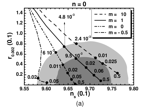
Plot	(a): $n=0$ & $m$ Equal to:				(b): $m=1$ & $n$ Equal to:
	$-0.5$	$0$	$1$	$10$	$-0.1$	$0$	$0.1$	$0.2$
$r_{\pm}^{\rm min}/10^{-3}$	$20$	$6$	$4.8$	$2.4$	$5.8$	$4.8$	$4.2$	$3.7$
$r_{\pm}^{\rm max}$	$0.05$	$0.5$	$0.5$	$0.5$	$0.5$	$0.5$	$0.125$	$0.032$
$r_{0.002}^{\rm min}/10^{-3}$	$3.9$	$1.9$	$6.5$	$23$	$25$	$6.5$	$3.5$	$7.9$

Figure 1: Allowed curves in the $n_{\rm s}-r_{0.002}$ plane for $n=0$ and $m=-1,0,1,10$ (a) or $m=1$ and $n=-0.1,0,0.1,0.2$ (b) with the $r_{\pm}$ values indicated on the curves. The conventions adopted for the various lines are also shown. The marginalized joint $68\%$ [$95\%$] regions from Planck, Bicep2/Keck Array and BAO data are depicted by the dark [light] shaded contours. The allowed $r_{\pm}^{\rm min}$ and $r_{\pm}^{\rm max}$ together with the minimal $r_{0.002}$, $r_{0.002}^{\rm min}$, in each case are listed in the table.

We start the presentation of our results by comparing the outputs of our models against the observational data [8, 10] in the $n_{\rm s}-r_{0.002}$ plane – see Fig. 1. We depict the theoretically allowed values with dot-dashed, double dot-dashed, solid and dashed lines respectively for (i) $n=0$ and $m=-0.5,0,1$ and $10$ in Fig. 1-(a) or (ii) $m=1$ and $n=1/5,1/10,0$ and $-1/10$ in Fig. 1-(b). The variation of $r_{\pm}$ is shown along each line. In both plots, for low enough $r_{\pm}$’s – i.e. $r_{\pm}\leq 0.0005$ – the various lines converge to $(n_{\rm s},r_{0.002})\simeq(0.947,0.28)$ obtained within quatric inflation defined for $c_{+}=0$. Increasing $r_{\pm}$ the various lines enter the observationally allowed regions, for $r_{\pm}$ equal to a minimal value $r_{\pm}^{\rm min}$, and cover them. The lines corresponding to $n=0$ and $m=0,1,10$ or $m=1$ and $n=0,-0.1$ terminate for $r_{\pm}=r_{\pm}^{\rm max}\simeq 0.5$, beyond which Eq. (15) is violated. The same origin has the termination point of the line corresponding to $n=0$ and $m=-0.5$ which occurs for $r_{\pm}=0.05$. Finally the lines drawn with $m=1$ and $n=1/5$ or $n=1/10$ cross outside the allowed corridors and so the $r_{\pm}^{\rm max}$’s, are found at the intersection points. More specifically, the values of $r_{\pm}^{\rm min}$ and $r_{\pm}^{\rm max}$ for any line depicted in Fig. 1, are accumulated in the Table shown below the plots – the entries of the fourth and seventh column coincide with each other, since in both cases we have $m=1$ and $n=0$.

From Fig. 1-(a) we deduce that increasing $m$ above $-0.5$ with $n=0$ the various curves move to the right. On the other hand, from Fig. 1-(b) we infer that for $m=1$ the lines with $n>0$ [$n<0$] cover the left lower [right upper] corner of the allowed range. Obviously for $m>1$ we expect that solutions with $n>0$ are preferable since they fill the observationally favored region – cf. Fig. 4 below. As we anticipated in Sec. 4.1, for $n>0$ nMHI is of hilltop type. The relevant parameter $\Delta_{\rm max\star}$ ranges from $0.07$ to $0.66$ for $n=1/10$ and from $0.19$ to $0.54$ for $n=1/5$ where $\Delta_{\rm max\star}$ increases as $r_{\pm}$ drops. That is, the required tuning is not severe mainly for $r_{\pm}<0.1$. In conclusion, the observationally favored region can be wholly filled varying conveniently $m$ for $n=0$ or $n$ for $m=1$.

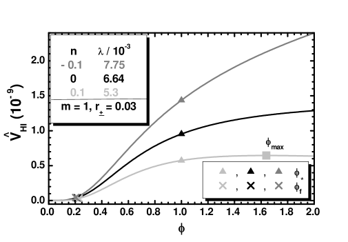
Figure 2: The inflationary potential $\widehat{V}_{\rm HI}$ as a function of $\phi$ for $\phi>0$ and $m=1$, $r_{\pm}\simeq 0.03$, and $n=-0.1$, $\lambda=7.75\cdot 10^{-3}$ (gray line), $n=0$, $\lambda=6.64\cdot 10^{-3}$ (black line), or $n=+0.1$, $\lambda=5.3\cdot 10^{-3}$ (light gray line). The values of $\phi_{\star}$, $\phi_{\rm f}$ and $\phi_{\rm max}$ (for $n=1/10$) are also indicated.

The structure of $\widehat{V}_{\rm HI}$ as a function of $\phi$ for $\phi_{\star}=1$, $r_{\pm}=0.03$, $m=1$ and $n=-0.1$ (light gray line), $n=0$ (black line) and $n=0.1$ (gray line) is displayed in Fig. 2. The corresponding values of $\lambda$ are $(7.75,6.64~{}{\rm or}~{}5.3)\cdot 10^{-3}$ with $c_{-}$ being calculated from Eq. (20) to be $(1.7,1.46,{\rm or}~{}1.24)\cdot 10^{2}$ whereas the corresponding observable quantities are found numerically to be $n_{\rm s}=0.971,0.969$ or $0.966$ and $r=0.045,0.03$ or $0.018$ with $a_{\rm s}\simeq-5\cdot 10^{-4}$ in all cases. These results are consistent with the analytic formulas of Sec. 4.2. Indeed, applying them we find $n_{\rm s}=0.97,0.969$ or $0.965$ and $r=0.047,0.031$ or $0.019$ in excellent agreement with the numerical outputs above. We observe that $\widehat{V}_{\rm HI}$ is a monotonically increasing function of $\phi$ for $n\leq 0$ whereas it develops a maximum at $\phi_{\rm max}=1.64$, for $n=0.1$, which leads to a mild tuning of the initial conditions of nMHI since $\Delta_{\rm max\star}=39\%$, according to the criterion discussed in Sec. 4.1. It is also remarkable that $r$ increases with the inflationary scale, $\widehat{V}_{\rm HI}^{1/4}$, which in all cases approaches the SUSY GUT scale $M_{\rm GUT}\simeq 8.2\cdot 10^{-3}$ as expected – see e.g. Ref. [38].

The relatively high $r$ values encountered here are associated with transplanckian values of $\widehat{\phi}_{\star}$ in accordance with the Lyth bound [39]. Indeed, in all cases $\widehat{\phi}_{\star}\simeq\sqrt{c_{-}}\phi_{\star}>1$ as can be derived from Eq. (30). This fact, though, does not invalidate our scenario since $\Phi$ and $\bar{\Phi}$ remain subplanckian thanks to Eq. (28b) which is satisfied imposing a lower bound on $c_{-}$ – see e.g. Eq. (37) – although $\widehat{\phi}_{\star}>1$. A second implication of Eq. (28b) is that although $\lambda/c_{-}$ is constant for fixed $r_{\pm}$, $n$ and $m$, the amplitudes of $\lambda$ and $c_{-}$ can be bounded. E.g., for $n=0,m=1$ and $r_{\pm}=0.03$ we obtain $146\lesssim c_{-}\lesssim 7\cdot 10^{6}$ for $6.6\cdot 10^{-4}\lesssim\lambda\lesssim 3.5$, where the upper bound ensures that $\lambda$ stays within the perturbative region.

Concentrating on the most promising cases with $n=0$ or $m=1$, we delineate, in Fig. 3, the allowed regions of our models by varying continuously $r_{\pm}$ and $m$ for $n=0$, in Fig. 3-(a), or $n$ for $m=1$, in Fig. 3-(b). The conventions adopted for the various lines are also shown in the figure. In particular, the allowed (shaded) regions are bounded by the dashed line, which originates from Eq. (15), and the dot-dashed and thin lines along which the lower and upper bounds on $n_{\rm s}$ and $r$ in Eq. (21) are saturated respectively. We remark that increasing $r_{\pm}$, with $n=0$ and fixed $m$, $r$ decreases, in accordance with our findings in Fig. 1-(a). On the other hand, for $m=1$, $r_{\pm}$ takes more natural – in the sense of the discussion below Eq. (4g) – values (lower than unity) for larger values of $|n|$ where hilltop nMHI is activated. Fixing $n_{\rm s}$ to its central value in Eq. (21) we obtain the thick solid lines along which we get clear predictions for $m$ in Fig. 3-(a) or $n$ in Fig. 3-(b), $r_{\pm}$ and the remaining inflationary observables. Namely, from Fig. 3-(a), for $n=0$ and ${\widehat{N}_{\star}}\simeq 58$, we obtain

$$0.2\lesssim m\lesssim 4,\>\>\>0.064\lesssim{r_{\pm}\over 0.1}\lesssim 5,\>\>\>0.29\lesssim{r\over 0.01}\lesssim 7\>\>\>\mbox{and}\>\>\>0.28\lesssim 10^{5}{\lambda\over c_{-}}\lesssim 1.9\,.$$ (46a)

Comparing Fig. 3-(a) with Fig. 2 of Ref. [3] we see that the latest [10] upper bound on $$r m\gtrsim-0.6 n_{\rm s}=0.968 m=1 {\widehat{N}_{\star}}\simeq 58$$ in Eq. (21) cuts the lower right slice from the allowed region and consequently a part from the solid line. Also the allowed region is limited to since below this value Eq. (15) is broken, as we now recognize. Similarly, from Fig. 3-(b), for , and we find

$$-1.21\lesssim{n\over 0.1}\lesssim 0.215,\>\>\>0.12\lesssim{r_{\pm}\over 0.1}\lesssim 5,\>\>\>0.4\lesssim{r\over 0.01}\lesssim 7\>\>\>\mbox{and}\>\>\>0.25\lesssim 10^{5}{\lambda\over c_{-}}\lesssim 2.6\,.$$ (46b)

Hilltop nMHI is attained for $0<n\leq 0.0215$ and there, we get $\Delta_{\rm max\star}\gtrsim 0.4$. In both cases above $a_{\rm s}$ is confined in the range $-(5-6)\cdot 10^{-4}$ and so, our models are consistent with the fitting of data with the $\Lambda$CDM+$r$ model [8]. Moreover, our models are testable by the forthcoming experiments [41] searching for primordial gravity waves since $r\gtrsim 0.0019$.

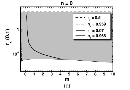
Figure 3: Allowed (shaded) regions in the $n-r_{\pm}$ plane for $n=0$ (a) and $m=1$ (b). The conventions adopted for the various lines are also shown.

Had we employed $K_{i}$ with $i=1,2$, the various lines ended at $r_{\pm}\simeq 0.5$ in Fig. 1 and the allowed regions in Fig. 3 would have been shortened until $r_{\pm}\simeq 1/3$. This bound would have yielded slightly larger $r_{0.002}^{\rm min}$’s. Namely, $r_{0.002}^{\rm min}/10^{-3}\simeq 2.8,8.4$ and $25$ for $n=0$ and $m=0,1$ and $10$ whereas $r_{0.002}^{\rm min}\simeq 0.026$ for $m=1$ and $n=-0.1$ – the $r_{0.002}^{\rm min}$’s for $n>0$ are let unaffected. For $n=0$ and $m=-0.5$ we obtain $r_{\pm}^{\rm max}\simeq 0.04$ and $r_{0.002}^{\rm min}\simeq 0.0045$. The lower bound of $r/0.01$ and the upper ones on $r_{\pm}/0.1$ and $10^{5}\lambda/c_{-}$ in Eq. (46a) [Eq. (46b)] become $0.42$, $3.3$ and $1.5$ [$0.64$, $3.3$ and $2.1$] whereas the bounds on $a_{\rm s}$ remain unaltered.

Fixing $r_{\pm}$ to some representative value, we can delineate the allowed region of our models in the $m-n$ plane as shown in Fig. 4. Namely we set $r_{\pm}=0.008$ in Fig. 4-(a) and $r_{\pm}=0.03$ in Fig. 4-(b). We use the same shape code for the the boundary lines of the allowed (shaded) regions as in Fig. 3. Particularly, the dot-dashed thick line corresponds to the lower bound on $n_{\rm s}$ in Eq. (21a) whereas the thin line comes from Eq. (21b). Along the solid thick line the central value of $n_{\rm s}$ in Eq. (21a) is attained. We see that the largest parts of the allowed regions are found for $n>0$ which means that nMHI is of hilltop type. Moreover, comparing Fig. 4-(a) and Fig. 4-(a) we remark that the $n>0$ slice of the allowed region is extended as $r_{\pm}$ decreases. In all, for $n_{\rm s}=0.968$ we take:

$$2.3\lesssim{r/0.01}\lesssim 7\>\>\>\mbox{with}\>\>\>-0.08\lesssim n\lesssim 1.69\>\>\>\mbox{and}\>\>\>2\lesssim{m}\lesssim 10\,\>\>\>(r_{\pm}=0.008);$$ (47a)

$$1.2\lesssim{r/0.01}\lesssim 2.2\>\>\>\mbox{with}\>\>\>-0.0135\lesssim n\lesssim 1.46\>\>\>\mbox{and}\>\>\>0\lesssim{m}\lesssim 10\,\>\>\>(r_{\pm}=0.03).$$ (47b)

From the relevant plots we observe that $n$ increases with $m$ along the bold solid line. Hilltop nMHI is attained for $m\geq 3$ with $\Delta_{\rm max\star}\gtrsim 0.26$ for $r_{\pm}=0.008$ and for $m\geq 0.45$ with $\Delta_{\rm max\star}\gtrsim 0.58$ for $r_{\pm}=0.03$. In both cases, $\Delta_{\rm max\star}$ (and $r$) decreases as $m$ increases.

As we mention in Sec. 4.1, $\widehat{m}_{\rm\delta\phi}$ is affected heavily from the choice of $K$’s in Eqs. (4a) – (4g) as $r_{\pm}$ approaches its upper bound in Eq. (15). Particularly, if we employ $K_{i}$ with $i=3,...,7$ along the bold solid lines in Fig. 3-(a) and Fig. 3-(b) we obtain

$$2.4\cdot 10^{-3}\lesssim{\widehat{m}_{\rm\delta\phi}/10^{-5}}\lesssim 1.2\,\>\>\>\mbox{and}\>\>\>2.1\cdot 10^{-3}\lesssim{\widehat{m}_{\rm\delta\phi}/10^{-5}}\lesssim 1.5\,$$ (48a)

respectively, whereas for $$i=1,2 2.6\cdot 10^{-2} 2.4\cdot 10^{-2}$$ the upper bounds above remain unchanged and the lower bounds move on to and correspondingly. On the other hand, along the bold solid lines in Fig. 4-(a) and Fig. 4-(b) we obtain

$$2\lesssim{\widehat{m}_{\rm\delta\phi}/10^{-8}}\lesssim 4.9\,\>\>\>\mbox{and}\>\>\>2.9\lesssim{\widehat{m}_{\rm\delta\phi}/10^{-8}}\lesssim 12\,$$ (48b)

respectively, with the bounds being independent from the choice of $K$. These $\widehat{m}_{\rm\delta\phi}$ ranges let open the possibility of non-thermal leptogenesis [40] if we introduce a suitable coupling between $\bar{\Phi}$ and the right-handed neutrinos – see e.g. Refs. [25, 14].

Figure 4: Allowed (shaded) region in the $m-n$ plane for $r_{\pm}=0.008$ (a) and $r_{\pm}=0.03$ (b). The conventions adopted for the various lines are also shown.

Setting $m=1$ in Eqs. (4b), (4d), (4f) or (4g) and $n=0$ – i.e. $N_{2}=3$ in Eq. (4b) or $N_{i}=2$ with $i=4,6,7$ in Eqs. (4d), (4f) and (4g) – we can construct the most economical and predictive version of our models which evades higher order terms of the form $(1+c_{+}F_{+})^{m-1}$ and the relevant tuning on $n$. In this restrictive case, $n_{\rm s}=0.968$ – see Eq. (21) – entails $r_{\pm}=0.015$ and corresponds to $r=0.043$ which is a little higher than the central observational value – see details below Eq. (21) – but still within the $65\%$ c.l favored margin [10]. Moreover, Eq. (15) implies $r_{0.002}^{\rm min}\simeq 0.0065$ – see Fig. 1. The alternative minimalistic choice $m=n=0$ which avoids higher order terms in Eqs. (4a), (4c) and (4e) do not yield solutions with $n_{\rm s}=0.968$ – see Fig. 3-(a).

5 Conclusions

Extending our work in Refs. [1, 2, 3] we analyzed further the implementation of kinetically modified nMHI within SUGRA. We specified seven Kähler potentials $K_{i}$ with $i=1,...,7$, see Eqs. (4a) – (4g), which cooperate with the well-known simplest superpotential $W$ in Eq. (2) leading to $\widehat{V}_{\rm HI}$, collectively given in Eq. (10), and a GUT phase transition at the SUSY vacuum in Eq. (7). Prominent in the proposed $K$’s is the role of a shift-symmetric quadratic function $F_{-}$ in Eq. (3) which remains invisible in $\widehat{V}_{\rm HI}$ while dominates the canonical normalization of the Higgs-inflaton. On the other hand, we employ two stabilization mechanisms for the non-inflaton field $S$, one with higher order terms, in Eqs. (4a) – (4d), and one leading to a $SU(2)_{S}/U(1)$ symmetric Kähler manifold in Eqs. (4e) – (4g). In all, our inflationary setting depends essentially on four free parameters ($n$, $m$, $\lambda/c_{-}$ and $r_{\pm}$), where $n$ and $r_{\pm}$ are defined in terms of the initial variables as shown in Eqs. (12) and (15) respectively. The model parameters are constrained to natural values, imposing a number of observational and theoretical restrictions. Predictions on $r$ value, testable in the near future, were also obtained.

More specifically, for $n=0$ we updated the results of Ref. [3] in Fig. 1-(a) and Fig. 3-(a). For $n\neq 0$ and $m=1$, we found new allowed regions presented in Fig. 1-(b) and Fig. 3-(b). Especially for $n>0$, we showed that $\widehat{V}_{\rm HI}$ develops a maximum which does not disturb, though, the implementation of hilltop nMHI since the relevant tuning is mostly very low. Indicatively, fixing $n_{\rm s}\simeq 0.968$ and $n=0$, or $m=1$, or $r_{\pm}=0.008$, or $r_{\pm}=0.03$ we obtained the outputs in Eq. (46a) or Eq. (46b) or Eq. (47a) or Eq. (47b) respectively. The majority of these solutions can be classified in the hilltop branch as shown in Fig. 4 where we varied continuously $n$ and $m$ with fixed $r_{\pm}$.

In all cases, $\lambda/c_{-}$ is computed enforcing Eq. (20) and $|a_{\rm s}|$ turns out to be negligibly small. Our inflationary setting can be attained with subplanckian values of the initial (non-canonically normalized) inflaton, requiring large $c_{-}$’s, without causing any problem with the perturbative unitarity. It is gratifying, finally, that our proposal remains intact from radiative corrections, the Higgs-inflaton may assume ultimately the v.e.v predicted by the gauge unification within MSSM, and the inflationary dynamics can be studied analytically and rather accurately for $n=0$ and $m\geq 0$ or $m=1$ and any $n$.

Finally, we would like to point out that, although we have restricted our discussion on the $G_{\rm GUT}=G_{\rm SM}\times U(1)_{B-L}$ gauge group, kinetically modified nMHI analyzed in this paper has a much wider applicability. It can be realized within other GUTs, provided that $\Phi$ and $\bar{\Phi}$ consist a conjugate pair of Higgs superfields. If we adopt another GUT gauge group, the inflationary predictions are expected to be quite similar to the ones discussed here with possibly different analysis of the stability of the inflationary trajectory, since different Higgs superfield representations may be involved in implementing the $G_{\rm GUT}$ breaking to $G_{\rm SM}$. Removing the scale $M$ from $W$ in Eq. (2) and abandoning the idea of grand unification, our inflationary stage can be realized even by the electroweak higgs boson – cf. Ref. [18]. Since our main aim here is the observational investigation of the kinetically modified nMHI, we opted to utilize the simplest GUT embedding.