New formulas for $\pi$ involving infinite nested square roots and Gray code.

Abstract.

In previous papers we introduced a class of polynomials which follow the same recursive formula as the Lucas-Lehmer numbers, studying the distribution of their zeros and remarking that this distribution follows a sequence related to the binary Gray code. It allowed us to give an order for all the zeros of every polynomial $L_{n}$. In this paper, the zeros, expressed in terms of nested radicals, are used to obtain two formulas for $\pi$: the first can be seen as a generalization of the known formula

$$\pi=\lim_{n\rightarrow\infty}2^{n+1}\cdot\sqrt{2-\underbrace{\sqrt{2+\sqrt{2+\sqrt{2+...+\sqrt{2}}}}}_{n}}\ ,$$

related to the smallest positive zero of $L_{n}$; the second is an exact formula for $\pi$ achieved thanks to some identities valid for $L_{n}$.

1. Introduction.

In this paper we obtain $\pi$ as the limit of a sequence related to the zeros of the class of polynomials $L_{n}(x)=L_{n-1}^{2}(x)-2$ created by means of the same iterative formula used to build the well-known Lucas-Lehmer sequence, employed in primality tests Bressoud (1989); Finch (2003); Koshy (2001); Lehmer (1930); Lucas (1878a, c, b); Ribenboim (1988). This class of polynomials was introduced in previous papers Vellucci and Bersani (2016a), Vellucci and Bersani (2016c).

The results obtained here are based on the placement of the zeros of the polynomials $L_{n}(x)$, studied in Vellucci and Bersani (2016b), and generalize the well-known relation

(1) $$\pi=\lim_{n\rightarrow\infty}2^{n+1}\cdot\sqrt{2-\underbrace{\sqrt{2+\sqrt{2+\sqrt{2+...+\sqrt{2}}}}}_{n}}\ .$$

Zeros have a structure of nested radicals, by means of which we can build infinite sequences of nested radicals converging to $\pi$. The ordering of the zeros follows the sequence of the binary Gray code, which is very useful in computer science and in telecommunications Vellucci and Bersani (2016b).

Starting from the seminal papers by Ramanujan (Ramanujan (2000), Berndt (1989) pp. 108-112), there is a vast literature studying the properties of the so-called continued radicals as, for example: Herschfeld (1935); Jonathan M. Borwein (1991); Sizer (1986); Johnson and Richmond (2008); Efthimiou (2013); Lynd (2014). Other authors investigated the properties of more general continued operations and their convergence. For a nice review of these results, see for example Jones (2015), which focuses mainly on continued reciprocal roots.

The nested square roots of 2 are a special case of the wide class of continued radicals. They have been studied by several authors. In particular, Cipolla Cipolla (1908) obtained a very elegant formula for

$$\sqrt{2+i_{n}\sqrt{2+i_{n-1}\sqrt{2+\cdots+i_{1}\sqrt{2}}}}\,,$$

in terms of $2\cos\left(k_{n}\frac{\pi}{2^{n+2}}\right)$, where $i_{k}\in\{-1,1\}$ and $k_{n}$ is a constant depending on $i_{1}$, $\dots$, $i_{n}$.

Servi Servi (2003) rediscovered and extended Cipolla’s formula, tying the evaluation of nested square roots of the form

(2) $$R(b_{k},...,b_{1})=\frac{b_{k}}{2}\sqrt{2+b_{k-1}\sqrt{2+b_{k-2}\sqrt{2+...+b_{2}\sqrt{2+2\sin\left(\frac{b_{1}\pi}{4}\right)}}}}$$

where $b_{i}\in\{-1,0,1\}$ for $i\neq 1$, to expression

(3) $$\left(\frac{1}{2}-\frac{b_{k}}{4}-\frac{b_{k}b_{k-1}}{8}-...-\frac{b_{k}b_{k-1}...b_{1}}{2^{k+1}}\right)\pi$$

to obtain, amongst other results, some nested square roots representations of $\pi$:

(4) $$\pi=\lim_{k\rightarrow\infty}\left[\frac{2^{k+1}}{2-b_{1}}R\left(\underbrace{1,-1,1,1,\dots,1,1,b_{1}}_{k\ \text{terms}}\right)\right]$$

where $b_{1}\neq 2$. Nyblom Nyblom (2005), citing Servi’s work, derived a closed-form expression for (2) with a generic $x\geq 2$ that replaces $2\sin\left(\frac{b_{1}\pi}{4}\right)$ in (2). Efthimiou Efthimiou (2012) proved that the radicals

$$a_{0}\sqrt{2+a_{1}\sqrt{2+a_{2}\sqrt{2+a_{3}\sqrt{2+\cdots}}}},\ \ a_{i}\in\{-1,1\}$$

have limits two times the fixed points of the Chebyshev polynomials $T_{2^{n}}(x)$, unveiling an interesting relation between these topics. The previous formula is equivalent to

(5) $$\pm\sqrt{2\pm\sqrt{2\pm\sqrt{2\pm\sqrt{2\pm...\pm\sqrt{2}}}}}\,.$$

In Moreno and García-Caballero (2012, 2013), the authors report a relation between the nested square roots of depth $n$ as $\pm\sqrt{2\pm\sqrt{2\pm\sqrt{2\pm\cdots\pm\sqrt{2+2z}}}}$, $z\in\mathbb{C}$ and the Chebyshev polynomials of degree $2^{n}$ in a complex variable, generalizing and unifying Servi and Nyblom’s formulas. In Moreno and García-Caballero (2012), the authors propose an ordering of the continued roots

(6) $$b_{k}\sqrt{2+b_{k-1}\sqrt{2+\cdots+b_{1}\sqrt{2+2\xi}}}\ ,$$

where $\xi=1$ and each $b_{i}$ is either $1$ or $-1$, according to formula

(7) $$j(b_{k},\dots,b_{1})=\frac{1}{2}\left(2^{k}-\left(\sum_{j=1}^{k}\left(2^{k-j}\prod_{i=0}^{j-1}b_{k-i}\right)\right)+1\right),$$

for each positive integer $k$. Formula (6) expresses the nested square roots of 2 in (5), and in Vellucci and Bersani (2016b) we gave an alternative ordering for them involving the so-called Gray code which, to the best of our knowledge, is applied for the first time to these topics.

Actually, there is a strong connection between Moreno and García-Caballero (2012) and Vellucci and Bersani (2016b). From (7), we have, for example: $j(1,1,1)=1$, $j(1,1,-1)=2$, $j(1,-1,-1)=3$, $j(1,-1,1)=4$, $j(-1,-1,1)=5$, j(-1,-1,-1) =6, $j(-1,1,-1)=7$ and $j(-1,1,1)=8$. If we associate bit $0$ to number $b_{i}=1$ and bit $1$ to number $b_{i}=-1$, in the expression of index $j$, we obtain

$$(1,1,1) \ \ \mapsto\ \ (0,0,0)$$

$$(1,1,-1) \ \ \mapsto\ \ (0,0,1)$$

$$(1,-1,-1) \ \ \mapsto\ \ (0,1,1)$$

$$(1,-1,1) \ \ \mapsto\ \ (0,1,0)$$

$$(-1,-1,1) \ \ \mapsto\ \ (1,1,0)$$

$$(-1,-1,-1) \ \ \mapsto\ \ (1,1,1)$$

$$(-1,1,-1) \ \ \mapsto\ \ (1,0,1)$$

$$(-1,1,1) \ \ \mapsto\ \ (1,0,0)\ ,$$

which are just an example of Gray code.

In this paper, after having recalled in Section 2 the most important definitions and properties of the Lucas-Lehmer polynomials, in Section 3 we extend formula (4), using the properties of the zeros of these polynomials (shown in Vellucci and Bersani (2016b)), stating and proving Theorem 3.3, which produces infinite numerical sequences converging to $\pi$. Besides, under suitable assumptions, Proposition 3.2 simplifies the expression of (3) listed in Servi’s Theorem (Servi (2003), formula (8)).

We also show that the generalizations of the Lucas-Lehmer map, $M_{n}^{a}$ for $a>0$ introduced in Vellucci and Bersani (2016a), have the same properties of $L_{n}$, for what concerns the distribution of the zeros and the approximations of $\pi$. We also obtain $\pi$ not as the limit of a sequence, but equal to an expression involving the zeros of the polynomials $L_{n}$ and $M_{n}^{a}$ for $a>0$.

Some perspectives of future applications of our results are reported in Section 4.

2. Preliminaries.

In this section we recall properties and useful results from our previous papers (Vellucci and Bersani (2016c), Vellucci and Bersani (2016a), Vellucci and Bersani (2016b)), and therefore we will list them without proofs.

2.1. The class of Lucas-Lehmer polynomials

We recall below some basic facts about Lucas-Lehmer polynomials

(8) $$L_{0}(x)=x\quad;\quad L_{n}(x)=L_{n-1}^{2}-2\ \ \forall n\geq 1$$

taken from Vellucci and Bersani (2016a). The polynomials $L_{n}(x)$ are orthogonal with respect to the weight function

$$\frac{1}{4\sqrt{4-x^{2}}}$$

defined on $x\in(-2,2)$.

Besides, for each $n\geq 1$ we have

(9) $$L_{n}(x)=2\ T_{2^{n-1}}\left(\frac{x^{2}}{2}-1\right)$$

where the Tchebycheff polynomials of first kind Bateman et al. (1955); Rivlin (1990) satisfy the recurrence relation

$$\begin{cases}T_{n}(x)=2xT_{n-1}(x)-T_{n-2}(x)\qquad n\geq 2\\ T_{0}(x)=1,\ \ T_{1}(x)=x\\ \end{cases}$$

from which it easily follows that for the $n$-th term:

(10) $$T_{n}(x)=\frac{\left(x-\sqrt{x^{2}-1}\right)^{n}+\left(x+\sqrt{x^{2}-1}\right)^{n}}{2}\,.$$

This formula is valid in $\mathbb{R}$ for $|x|\geq 1$; here we assume instead that $T_{n}$, defined in $\mathbb{R}$, can take complex values, too. Let $x=2\cos\theta$, then the polynomials $L_{n}(x)$ admit the representation

(11) $$L_{n}(2\cos\theta)=2\cos\left(2^{n}\theta\right)\,.$$

When $|x|\leq 2$, we can write $x=2\cos(\vartheta)$, thus $\displaystyle\frac{x^{2}}{2}-1=\cos(2\vartheta)$; hence, for $|x|\neq\sqrt{2}$, we can also put

(12) $$\vartheta(x)=\frac{1}{2}\arctan\left[\frac{\sqrt{1-\left(\frac{x^{2}}{2}-1\right)^{2}}}{\frac{x^{2}}{2}-1}\right]+b\pi$$

where $b$ is a binary digit; thus, using (11), we obtain

(13) $$L_{n}(x)=2\cos\left(2^{n}\vartheta(x)\right)\ .$$

Moreover, since $L_{1}(\pm\sqrt{2})=0\ ;\ L_{2}(\pm\sqrt{2})=-2\ ;\ L_{n}(\pm\sqrt{2})=2\quad\forall n\geq 3\$, then the argument of $L_{n}(\pm\sqrt{2})$ is $0$ for every $n\geq 3$.

By setting further

(14) $$\theta(x)=\frac{1}{2}\arctan\left[\frac{\sqrt{1-\left(\frac{x^{2}}{2}-1\right)^{2}}}{\frac{x^{2}}{2}-1}\right]$$

we can write:

(15) $$L_{n}(x)=2\cos\left(2^{n}\theta(x)+2^{n}b\pi\right)=2\cos\left(2^{n}\theta(x)\right)\ .$$

Like those of the first kind, Tchebycheff polynomial of second kind are defined by a recurrence relation  Bateman et al. (1955); Rivlin (1990):

$$\begin{cases}U_{0}(x)=1,\ \ U_{1}(x)=2x\\ U_{n}(x)=2xU_{n-1}(x)-U_{n-2}(x)\quad\forall n\geq 2\,,\\ \end{cases}$$

which is satisfied by

(16) $$U_{n}(x)=\sum_{k=0}^{n}(x+\sqrt{x^{2}-1})^{k}(x-\sqrt{x^{2}-1})^{n-k}\quad\forall x\in[-1,1]\ .$$

This relation is equivalent to

(17) $$U_{n}(x)=\frac{\left(x+\sqrt{x^{2}-1}\right)^{n+1}-\left(x-\sqrt{x^{2}-1}\right)^{n+1}}{2\sqrt{x^{2}-1}}$$

for each $x\in(-1,1)$. From continuity of function (16), we observe that (17) can be extended by continuity in $x=\pm 1$, too.

It can therefore be put $U_{n}(\pm 1)=(\pm 1)^{n}(n+1)$ in (17). From Vellucci and Bersani (2016a), for each $n\geq 1$ we have

(18) $$\prod_{i=1}^{n}L_{i}(x)=U_{2^{n}-1}\left(\frac{x^{2}}{2}-1\right)$$

and

(19) $$\prod_{i=1}^{n}L_{i}(2\cos\theta)=\frac{\sin\left(2^{n+1}\theta\right)}{\sin 2\theta}\ .$$

2.2. An ordering for zeros of Lucas-Lehmer polynomials using Gray code.

Given a binary code, its order is the number of bits with which the code is built, while its length is the number of strings that compose it. The celebrated Gray code Gardner (1986); Nijenhuis and Wilf (1978) is a binary code of order $n$ and length $2^{n}$.

Figure 1. Sub-codes for $m=2$, $m=3$.

We recall below how a Gray Code is generated; if the code for $n-1$ bit is formed by binary strings

$$\begin{array}[]{l}g_{n-1,1}\\ \vdots\\ g_{n-1,2^{n-1}-1}\\ g_{n-1,2^{n-1}}\ ,\end{array}$$

the code for $n$ bits is built from the previous one in the following way:

$$\begin{array}[]{l}0g_{n-1,1}\\ \vdots\\ 0g_{n-1,2^{n-1}-1}\\ 0g_{n-1,2^{n-1}}\\ 1g_{n-1,2^{n-1}}\\ 1g_{n-1,2^{n-1}-1}\\ \vdots\\ 1g_{n-1,1}\ .\end{array}$$

Just as an example, we have, for $n=1$: $g_{1,1}=0\ ;\ g_{1,2}=1$; for $n=2$: $g_{2,1}=00\ ;\ g_{2,2}=01\ ;\ g_{2,3}=11\ ;\ g_{2,4}=10$; for $n=3$:

$$g_{3,1} =000 g_{3,2} =001 g_{3,3} =011 g_{3,4} =010$$

(20) $$g_{3,5} =110 g_{3,6} =111 g_{3,7} =101 g_{3,8} =100\ ,$$

and so on.

Following the notation introduced in Vellucci and Bersani (2016b), we recall some preliminaries about Gray code.

Definition 2.1.

Let us consider a Gray code of order $n$ and length $2^{n}$. A sub-code is a Gray code of order $m<n$ and length $2^{m}$.

Definition 2.2.

Let us consider a Gray code of order $n$ and length $2^{n}$. An encapsulated sub-code is a sub-code built starting from the last string of Gray code of order $n$ that contains it.

Figure (1) contains some examples of encapsulated sub-codes inside a Gray code (with order $4$ and length $16$).

Let us consider the signs “plus” and “minus” in the nested form that expresses generic zeros of $L_{n}$, as follows:

(21) $$\sqrt{2\pm\underbrace{\sqrt{2\pm\sqrt{2\pm\sqrt{2\pm...\pm\sqrt{2\pm\sqrt{2}}}}}}}\,.$$

The underbrace encloses $n-1$ signs “plus” or “minus”, each one placed before each nested radical. Starting from the first nested radical we apply a code (i.e., a system of rules) that associates bits $0$ and $1$ to “plus” and “minus” signs, respectively.

Obviously, it is possible to obtain $2^{n-1}$ strings formed by $n-1$ bits. Let us define with $\displaystyle\{\omega(g_{n-1,j})\}_{j=1,...,2^{n-1}}$ the set of all the $2^{n-1}$ nested radicals of the form

$$2\pm\underbrace{\sqrt{2\pm\sqrt{2\pm\sqrt{2\pm...\pm\sqrt{2\pm\sqrt{2}}}}}}_{n-1\ \ signs}\,,$$

where each element of the set differs from the others for the sequence of “plus” and “minus” signs, and the index $j$ determines the position of the nested radical by virtue of Gray code.

3. Main results: $\pi$ formulas involving nested radicals.

3.1. Infinite sequences tending to $\pi$

Let us consider two finite sequences $x=\{x_{1},\dots,x_{n}\}$ and $y=\{y_{1},\dots,y_{m}\}$, $n,m\in\mathbb{N}$. We define the concatenation of these sequences the sequence $xy:=\{x_{1},\dots,x_{n},$ $y_{1},\dots,y_{n}\}$. Let us also consider the binary string $b_{n-m}$ composed by $n-m$ bits. The following results concern the set $\{\omega\left(b_{n-m}\,g_{m,h}\right)\}_{h=0}^{2^{m}-1}$. For example, in the following Lemma 3.1 we have $b_{n-m}=b_{2}=10$.

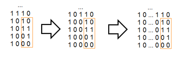
Figure 2. A possible subcode (orange), where the meaning of the limit (35) is highlighted: in this way the number of symbols 0, on the left of the sub-code, increases.

Lemma 3.1.

For all $m\in\mathbb{N}$ one has:

(22) $$\sqrt{\omega(10g_{m,h+1})}=2\sin\left(\frac{2h+1}{2^{m+4}}\pi\right)\ \ \ h\in\{0,1,\dots,2^{m}-1\}$$

Proof.

We proceed with induction principle for $m$ to prove (22). If $m=1$:

(23) $$\sqrt{\omega(10g_{1,h+1})}=2\sin\left(\frac{2h+1}{2^{5}}\pi\right)\ \ \ h\in\{0,1\}$$

i.e.

$$\sqrt{\omega(10g_{1,1})}=2\sin\left(\frac{\pi}{2^{5}}\right)$$

for $h=0$, and

$$\sqrt{\omega(10g_{1,2})}=2\sin\left(\frac{3\pi}{2^{5}}\right)$$

for $h=1$, where $g_{1,1}=0$ and $g_{1,2}=1$. These formulas are easy to check. Now we are going to check (22) for $m+1$:

(24) $$\sqrt{\omega(10g_{m+1,h+1})}=2\sin\left(\frac{2h+1}{2^{m+5}}\pi\right)\ \ \ h\in\{0,1,\dots,2^{m+1}-1\}$$

having assumed it true for $m\geq 1$. From Gray Code’s definition we have that either a) $g_{m+1,h+1}=0g_{m,h+1}$ or b) $g_{m+1,h+1}=1g_{m,2^{m}-h}$. In the former case:

$$\sqrt{\omega(10g_{m+1,h+1})}=\sqrt{\omega(100g_{m,h+1})}$$

where

$$\sqrt{\omega(100g_{m,h+1})} =\sqrt{2-\sqrt{\omega(00g_{m,h+1})}}$$

(25) $$=\sqrt{2-\sqrt{2+\sqrt{\omega(0g_{m,h+1})}}}\,.$$

But in fact: $\omega(10g_{m,h+1})=2-\sqrt{\omega(0g_{m,h+1})}$, so (3.1) becomes

$$\sqrt{\omega(100g_{m,h+1})} =\sqrt{2-\sqrt{2+\sqrt{\omega(0g_{m,h+1})}}}$$

$$=\sqrt{2-\sqrt{4-\omega(10g_{m,h+1})}}$$

$$=\sqrt{2-\sqrt{4-4\sin^{2}\left(\frac{2h+1}{2^{m+4}}\pi\right)}}$$

$$=\sqrt{2-2\cos\left(\frac{2h+1}{2^{m+4}}\pi\right)}$$

(26) $$=2\sin\left(\frac{2h+1}{2^{m+5}}\pi\right)\,.$$

Therefore (24) is proved for the case a).

Now we assume that $g_{m+1,h+1}=1g_{m,2^{m}-h}$:

$$\sqrt{\omega(10g_{m+1,h+1})}=\sqrt{\omega(101g_{m,2^{m}-h})}$$

thus

$$\sqrt{\omega(101g_{m,2^{m}-h})} =\sqrt{2-\sqrt{\omega(01g_{m,2^{m}-h})}}$$

$$=\sqrt{2-\sqrt{2+\sqrt{\omega(1g_{m,2^{m}-h})}}}$$

(27) $$=\sqrt{2-\sqrt{2+\sqrt{2-\sqrt{\omega(g_{m,2^{m}-h})}}}}$$

Noting that

$$\omega(0g_{m,2^{m}-h})=2+\sqrt{\omega(g_{m,2^{m}-h})}$$

it follows that

(28) $$\sqrt{\omega(101g_{m,2^{m}-h})}=\sqrt{2-\sqrt{2+\sqrt{4-\omega(0g_{m,2^{m}-h})}}}$$

From $\omega(10g_{m,2^{m}-h})=2-\sqrt{\omega(0g_{m,2^{m}-h})}$, equation (28) becomes

(29) $$\sqrt{\omega(101g_{m,2^{m}-h})}=\sqrt{2-\sqrt{2+\sqrt{4-\left[2-\omega(10g_{m,2^{m}-h})\right]^{2}}}}$$

From (22), we have

$$\sqrt{\omega(10g_{m,2^{m}-h})}=2\sin\left(\frac{2^{m+1}-(2h+1)}{2^{m+4}}\pi\right)$$

and equation (29) can be rewritten

$$\sqrt{\omega(101g_{m,2^{m}-h})} =\sqrt{2-\sqrt{2+\sqrt{4-\left[2-\omega(10g_{m,2^{m}-h})\right]^{2}}}}$$

$$=\sqrt{2-\sqrt{2+\sqrt{4-\left[2-4\sin^{2}\left(\frac{2^{m+1}-(2h+1)}{2^{m+4}}\pi\right)\right]^{2}}}}$$

$$=\sqrt{2-\sqrt{2+\sqrt{4-4\cos^{2}\left(\frac{2^{m+1}-(2h+1)}{2^{m+3}}\pi\right)}}}$$

$$=\sqrt{2-\sqrt{2+2\sin\left(\frac{2^{m+1}-(2h+1)}{2^{m+3}}\pi\right)}}$$

$$=\sqrt{2-\sqrt{2+2\cos\left(\frac{\pi}{2}-\frac{2^{m+1}-(2h+1)}{2^{m+3}}\pi\right)}}$$

(30) $$=\sqrt{2-2\cos\left(\frac{\pi}{4}-\frac{2^{m+1}-(2h+1)}{2^{m+4}}\pi\right)}\,.$$

Accordingly:

$$\sqrt{\omega(101g_{m,2^{m}-h})}=2\sin\left(\frac{2(h+2^{m})+1}{2^{m+5}}\pi\right)\,.$$

Since the term $h+2^{m}\in\{2^{m},\dots,2^{m+1}-1\}$ for $h\in\{0,\dots,2^{m}-1\}$, then (24) is fully shown and, with it, the whole proposition. ∎

Proposition 3.2.

For each $n\geq m+2$, $h\in\mathbb{N}$ such that $h\in\{0,1,\dots,2^{m}-1\}$:

(31) $$\sqrt{\omega(\bar{b}_{n-m}g_{m,h+1})}=2\sin\left(\frac{2h+1}{2^{n+2}}\pi\right)\,,$$

where $\bar{b}_{n-m}=10\dots 0$ has $n-m-1$ zeros.

Proof.

Put $n-m=\delta_{0}$, $n-m-1=\delta_{1}$, $n-m-2=\delta_{2}$, $\dots$, $n-m-k=\delta_{k}$ for $0\leq k\leq n-m-2$. Let us proceed by means of induction principle on $n$. Fixing $m$, suppose formula (31) to be true for a generic index $\delta_{1}$,

(32) $$\sqrt{\omega(\bar{b}_{\delta_{1}}g_{m,h+1})}=2\sin\left(\frac{2h+1}{2^{n+1}}\pi\right)\,,\quad\bar{b}_{\delta_{1}}=10\dots 0\,,$$

where $\bar{b}_{\delta_{1}}$ has $\delta_{1}-1$ zeros — and proceed to check the case $\delta_{0}$. We work on both sides of (32):

$$\omega(\bar{b}_{\delta_{1}}g_{m,h+1}) =4\sin^{2}\left(\frac{2h+1}{2^{n+1}}\pi\right)$$

$$2-\sqrt{\omega(\tilde{b}_{\delta_{2}}g_{m,h+1})} =4-4\cos^{2}\left(\frac{2h+1}{2^{n+1}}\pi\right)\,,$$

where $\tilde{b}_{\delta_{2}}=0\dots 0$. Then

$$-\sqrt{\omega(\tilde{b}_{\delta_{2}}g_{m,h+1})}=2-4\cos^{2}\left(\frac{2h+1}{2^{n+1}}\pi\right)$$

$$2+\sqrt{\omega(\tilde{b}_{\delta_{2}}g_{m,h+1})}=4\cos^{2}\left(\frac{2h+1}{2^{n+1}}\pi\right)$$

(33) $$\omega(\tilde{b}_{\delta_{1}}g_{m,h+1})=4\cos^{2}\left(\frac{2h+1}{2^{n+1}}\pi\right)\,,\quad\tilde{b}_{\delta_{1}}=0\tilde{b}_{\delta_{2}}\,,$$

whence

$$\sqrt{\omega(\tilde{b}_{\delta_{1}}g_{m,h+1})}=2\left|\cos\left(\frac{2h+1}{2^{n+1}}\pi\right)\right|=2\cos\left(\frac{2h+1}{2^{n+1}}\pi\right)\,.$$

Thus:

$$\sqrt{\omega(\tilde{b}_{\delta_{1}}g_{m,h+1})}=2\left(1-2\sin^{2}\left(\frac{2h+1}{2^{n+2}}\pi\right)\right)$$

or

$$2-\sqrt{\omega(\tilde{b}_{\delta_{1}}g_{m,h+1})}=4\sin^{2}\left(\frac{2h+1}{2^{n+2}}\pi\right)\,,$$

and

$$\omega(\bar{b}_{\delta_{0}}g_{m,h+1})=4\sin^{2}\left(\frac{2h+1}{2^{n+2}}\pi\right)\,,$$

hence

$$\sqrt{\omega(\bar{b}_{\delta_{0}}g_{m,h+1})}=2\left|\sin\left(\frac{2h+1}{2^{n+2}}\pi\right)\right|=2\sin\left(\frac{2h+1}{2^{n+2}}\pi\right).$$

Let us remark that $\bar{b}_{\delta_{0}}=\bar{b}_{n-m}=10\dots 0$ and it has $n-m-1$ zeros.

The absolute value can be removed by the proposition’s assumptions. Therefore, the inductive step is proved. Let us consider the base step: $\delta_{0}=2$. Indeed:

$$\sqrt{\omega(10g_{m,h+1})}=2\sin\left(\frac{2h+1}{2^{n-m+2}2^{m}}\pi\right)$$

or,

(34) $$\sqrt{\omega(10g_{m,h+1})}=2\sin\left(\frac{2h+1}{2^{m+4}}\pi\right)\ \ \ h\in\{0,1,\dots,2^{m}-1\}$$

which is proved, for all $m\in\mathbb{N}$, in Lemma 3.1. ∎

Theorem 3.3.

(35) $$\lim_{n\rightarrow\infty}\ \frac{2^{n+1}}{2h+1}\ \sqrt{\omega(\bar{b}_{n-m}g_{m,h+1})}=\pi$$

where $\bar{b}_{n-m}=10\dots 0$ has $n-m-1$ zeros, for every $h\in\mathbb{N}$ such that $h\in\{0,1,\dots,2^{m}-1\}$ and $n>m+1$.

Proof.

From Proposition 3.2, we have

(36) $$\frac{2^{n+1}}{2h+1}\ \sqrt{\omega(\bar{b}_{n-m}g_{m,h+1})}=\frac{2^{n+2}}{2h+1}\ \sin\left(\frac{2h+1}{2^{n+2}}\pi\right)$$

that, for a well-known limit, tends to $\pi$ for $n\to\infty$. ∎

Example 3.4.

With the help of computational tools we show below some iterations of a sequence described by

$$\frac{2^{n+1}}{2h+1}\ \sqrt{\omega(\bar{b}_{n-m}g_{m,h+1})}\,,$$

where $\bar{b}_{n-m}=10\dots 0$ has $n-m-1$ zeros.

Let us consider $m=3$; then

$$g_{3,1}=000\ ;\ g_{3,2}=001\ ;\ g_{3,3}=011\ ;\ g_{3,4}=010\ ;$$

$$g_{3,5}=110\ ;\ g_{3,6}=111\ ;\ g_{3,7}=101\ ;\ g_{3,8}=100.$$

We choose the binary string $g_{3,6}=111$; in this case, if $m=3$, one has $h+1=6$ and so $h=5$. This means that we are iterating

$$\frac{2^{n+1}}{11}\ \sqrt{\omega(\underbrace{10...0}_{n-3}111)}\,.$$

Hence, for $n=8$:

$$\frac{2^{9}}{11}\ \sqrt{\omega(10000111)}=$$

$$\frac{2^{9}}{11}\ \sqrt{2-\sqrt{2+\sqrt{2+\sqrt{2+\sqrt{2+\sqrt{2-\sqrt{2-\sqrt{2-\sqrt{2}}}}}}}}}\simeq 3.\textbf{14}0996\dots$$

For $n=12$:

$$\frac{2^{13}}{11}\ \sqrt{\omega(100000000111)}=$$

$$\frac{2^{13}}{11}\ \sqrt{2-\sqrt{2+\sqrt{2+\sqrt{2+\sqrt{2+\sqrt{2+\sqrt{2+\sqrt{2+\sqrt{2+\sqrt{2-\sqrt{2-\sqrt{2-\sqrt{2}}}}}}}}}}}}}$$

$$\simeq 3.\textbf{14159}0324\dots$$

and so on.

3.2. The generalized map $M^{a}_{n}=2a\left(M^{a}_{n-1}\right)^{2}-\frac{1}{a}$.

In Vellucci and Bersani (2016a) we introduced an extension of the map $L_{n}$, obtained through the iterated formula $M^{a}_{n}=2a\left(M^{a}_{n-1}\right)^{2}-\frac{1}{a}\ ,\ a>0$, with $M^{a}_{0}(x)=x$. It follows that

(37) $$M^{a}_{0}(x)=x\quad;\quad M^{a}_{1}(x)=2ax^{2}-\frac{1}{a}\quad;\quad M^{a}_{2}(x)=8a^{3}x^{4}-8ax^{2}+\frac{1}{a}\quad\dots.$$

Note that the map $L_{n}$ is a particular case of $M^{a}_{n}$, obtained by setting $a=1/2$. We briefly show that the map $M^{a}_{n}$ leads to the same $\pi$ formulas stated in the previous sections.

Proposition 3.5.

For $n\geq 2$ we have

(38) $$M^{a}_{n}(x)=\frac{1}{a}\cdot\cos(a\ 2^{n}x)+o(x^{2})\,.$$

Proof.

We must show that:

(39) $$M^{a}_{n}(x)=\frac{1}{a}-a2^{2n-1}x^{2}+o(x^{2})$$

where we take into account the McLaurin polynomial of cosine. We proceed by induction. For $n=2$:

(40) $$M^{a}_{2}(x)=2a\left(2ax^{2}-\frac{1}{a}\right)^{2}-\frac{1}{a}=\frac{1}{a}-8ax^{2}+o(x^{2})$$

Let us consider the second order McLaurin polynomial of $\frac{1}{a}\cdot\cos(4ax)$: it is just $\frac{1}{a}-8ax^{2}+o(x^{2})$, thus verifying the relation for $n=2$. Let us now assume (38) is true for a generic $n$, and deduce that it is also true for $n+1$:

$$M^{a}_{n+1}=2a\left(M^{a}_{n}\right)^{2}-\frac{1}{a}=2a\left[\frac{1}{a}-a2^{2n-1}x^{2}+o(x^{2})\right]^{2}-\frac{1}{a}=$$

(41) $$=\frac{1}{a}-a2^{2n+1}x^{2}+o(x^{2})$$

which is in fact the McLaurin polynomial of $\frac{1}{a}\cdot\cos(a\ 2^{n+1}x)$. ∎

Proposition 3.6.

At each iteration the zeros of the map $M^{a}_{n}(n\geq 1)$ have the form

(42) $$\pm\frac{1}{2a}\cdot\sqrt{2\pm\sqrt{2\pm\sqrt{2\pm\sqrt{2\pm...\pm\sqrt{2}}}}}\,.$$

Proof.

It is obvious that at $n=1$ this statement is valid.

Now assume that the (42) is valid for $n$. We have to prove that it is valid for $n+1$.

(43) $$2ax^{2}-\frac{1}{a}=\pm\frac{1}{2a}\cdot\sqrt{2\pm\sqrt{2\pm\sqrt{2\pm\sqrt{2\pm...\pm\sqrt{2}}}}}$$

or

(44) $$x^{2}=\frac{1}{2a^{2}}\pm\frac{1}{4a^{2}}\cdot\sqrt{2\pm\sqrt{2\pm\sqrt{2\pm\sqrt{2\pm...\pm\sqrt{2}}}}}$$

and placing under the radical sign

(45) $$x=\pm\sqrt{\frac{1}{2a^{2}}\pm\frac{1}{4a^{2}}\cdot\sqrt{2\pm\sqrt{2\pm\sqrt{2\pm\sqrt{2\pm...\pm\sqrt{2}}}}}}$$

the thesis is obtained. ∎

It is possible to prove that zeros of the map $M^{a}_{n+1}$ are related to those of $M^{a}_{n}$, $n\geq 1$.

3.3. $\pi$-formulas: not only approximations.

From (14) and (15) we obtained Vellucci and Bersani (2016a) the following formula:

(46) $$L_{n}(x)=2\cos\left[2^{n-1}\arctan\left(\frac{\sqrt{1-\left(\frac{x^{2}}{2}-1\right)^{2}}}{\frac{x^{2}}{2}-1}\right)\right]\,,$$

valid for $x\in[-2,2]$ and $x\neq\pm\sqrt{2}$. This expression is equivalent to

(47) $$L_{n}(x)=\left(\left(\left(x^{2}-2\right)^{2}-2\right)^{2}\ ...\ -2\right)^{2}-2$$

Moreover, we already observed that, for $|x|=\sqrt{2}$, we have

(48) $$L_{0}(\sqrt{2})=\sqrt{2}\quad;\quad L_{1}(\sqrt{2})=0\quad;\quad L_{2}(\sqrt{2})=-2\quad;\quad L_{n}(\sqrt{2})=2\ \ \forall n\geq 3\ .$$

The right hand side of (46) vanishes when

(49) $$2^{n-1}\arctan\left[\frac{\sqrt{1-\left(\frac{x^{2}}{2}-1\right)^{2}}}{\frac{x^{2}}{2}-1}\right]=\pm\frac{\pi}{2}\ (2h+1)\ ;\ h\in N\ ;\ x\neq\pm\sqrt{2}$$

i.e.,

(50) $$-\frac{\pi}{2}<\arctan\left[\frac{\sqrt{1-\left(\frac{x^{2}}{2}-1\right)^{2}}}{\frac{x^{2}}{2}-1}\right]=\pm\frac{\pi}{2^{n}}\ (2h+1)<\frac{\pi}{2}\quad,\quad x\neq\pm\sqrt{2}$$

whence

(51) $$\sqrt{1-\left(\frac{x^{2}}{2}-1\right)^{2}}=\left(\frac{x^{2}}{2}-1\right)T_{n,h}$$

where $T_{n,h}=\tan\left[\pm\frac{\pi}{2^{n}}\ (2h+1)\right]$, for $h=0,1,2...,h_{max}$, and $h_{max}$ defined in this way: from (49) and boundedness of inverse tangent function we have

$$\frac{\pi}{2^{n}}(2h+1)<\frac{\pi}{2}$$

from which

$$h<2^{n-2}-\frac{1}{2}$$

therefore $h_{max}=2^{n-2}-1$, for $n\geq 2$.

If the factor $T_{n,h}$ is negative, the solutions of (51) belong to the interval $(-\sqrt{2},\sqrt{2})$; otherwise $x\in[-2,-\sqrt{2})\ \cup\ (\sqrt{2},2]$, if $T_{n,h}>0$. We have:

(52) $$1-\left(\frac{x^{2}}{2}-1\right)^{2}=\ \left(\frac{x^{2}}{2}-1\right)^{2}T_{n,h}^{2}\ \Rightarrow\ \frac{x^{2}}{2}-1=\pm\frac{1}{\sqrt{1+T_{n,h}^{2}}}$$

Therefore we can write the zeros of $L_{n}$ in the form

(53) $$x^{n}_{h}=\pm\sqrt{2\pm\frac{2}{\sqrt{1+\tan^{2}\left[\frac{\pi}{2^{n}}\ (2h+1)\right]}}}\quad,\quad n\geq 2\ ;\ 0\leq h\leq 2^{n-2}-1$$

Moreover, we know that, for every $n\geq 2$, the $h$-th positive zero of $L_{n}(x)$ has the form:

(54) $$\sqrt{\omega(g_{n-1,2^{n-1}-h})}$$

where $0\leq h\leq 2^{n-2}-1$. Equating the two expressions, one finds:

(55) $$\frac{1}{1+\tan^{2}\left[\frac{\pi}{2^{n}}\ (2h+1)\right]}=\left[\frac{1}{2}\omega(g_{n-1,2^{n-1}-h})-1\right]^{2}$$

whence

(56) $$\pi=\frac{2^{n}}{2h+1}\arctan\sqrt{\frac{1}{\left[\frac{1}{2}\omega(g_{n-1,2^{n-1}-h})-1\right]^{2}}-1}\,,$$

for $n\geq 2$, $0\leq h\leq 2^{n-2}-1$. In this way we obtain infinitely many formulas giving $\pi$ not as the limit of a sequence, but through an equality involving the zeros of the polynomials $L_{n}$.

Similar considerations can be made for the polynomials $M^{a}_{n}$. Since, for $\displaystyle|x|\neq\frac{\sqrt{2}}{2a}$,

(57) $$M^{a}_{n}(x)=\frac{1}{a}\cos\left(2^{n-1}\arctan\left[\frac{\sqrt{1-\left(2a^{2}x^{2}-1\right)^{2}}}{2a^{2}x^{2}-1}\right]\right)$$

vanishes if

(58) $$2^{n-1}\arctan\left[\frac{\sqrt{1-\left(2a^{2}x^{2}-1\right)^{2}}}{2a^{2}x^{2}-1}\right]=\pm\frac{\pi}{2}\ (2h+1)$$

i.e.,

(59) $$\arctan\left[\frac{\sqrt{1-\left(2a^{2}x^{2}-1\right)^{2}}}{2a^{2}x^{2}-1}\right]=\pm\frac{\pi}{2^{n}}\ (2h+1)\ ,$$

then

(60) $$\sqrt{1-\left(2a^{2}x^{2}-1\right)^{2}}=\left(2a^{2}x^{2}-1\right)T_{n,h}$$

where $T_{n,h}=\tan\left[\pm\frac{\pi}{2^{n}}\ (2h+1)\right]$, with $h=0,1,2...,2^{n-2}-1$.

Furthermore:

(61) $$\left(2a^{2}x^{2}-1\right)\ T_{n,h}>0$$

The inequality $2a^{2}x^{2}-1>0$ is verified for $x<-\frac{\sqrt{2}}{2a}\ \vee\ x>\frac{\sqrt{2}}{2a}$. If $T_{n,h}$ is negative, the solutions of (60) belong to the interval $\left(-\frac{\sqrt{2}}{2a},\frac{\sqrt{2}}{2a}\right)$, otherwise $x\in\left[-\frac{1}{a},-\frac{\sqrt{2}}{2a}\right)\ \cup\ \left(\frac{\sqrt{2}}{2a},\frac{1}{a}\right]$, if $T_{n,h}>0$. On the other hand:

(62) $$1-\left(2a^{2}x^{2}-1\right)^{2}=T_{n,h}^{2}\ \left(2a^{2}x^{2}-1\right)^{2}\ \Rightarrow\ 2a^{2}x^{2}-1=\pm\frac{1}{\sqrt{1+T_{n,h}^{2}}}$$

from which:

(63) $$x_{h}^{n}=\pm\frac{1}{2a}\sqrt{2\pm\frac{2}{\sqrt{1+\tan^{2}\left[\frac{\pi}{2^{n}}\ (2h+1)\right]}}}$$

Since, from (42), the zeros of $M^{a}_{n}(x)$ are proportional to the zeros of $L_{n}(x)$, we can say that also the $2^{n-1}$ positive zeros of $M^{a}_{n}$, in decreasing order, follow the order given by the Gray code:

(64) $$\frac{1}{2a}\sqrt{\omega(g_{n-1,2^{n-1}-h})}$$

Equating the two expressions we find again the identity:

(65) $$\pi=\frac{2^{n}}{2h+1}\arctan\sqrt{\frac{1}{\left[\frac{1}{2}\omega(g_{n-1,2^{n-1}-h})-1\right]^{2}}-1}$$

4. Discussion and perspectives.

In previous papers (Vellucci and Bersani (2016a) and Vellucci and Bersani (2016b)) we introduced a class of polynomials which follow the same recursive formula as the Lucas-Lehmer numbers, studying the distribution of their zeros and remarking that this distributions follows a sequence related to the binary Gray code. It allowed us to give an order for all the zeros of every polynomial $L_{n}$, Vellucci and Bersani (2016b). In this paper, the zeros, expressed in terms of nested radicals, are used to obtain two formulas for $\pi$: the first (i.e., formula (35)) can be seen as a generalization of the known formula (1), because the latter can be seen as the case related to the smallest positive zero of $L_{n}$; the second (i.e., formula (56)) gives infinitely many formulas reproducing $\pi$ not as the limit of a sequence, but through an equality involving the zeros of the polynomials $L_{n}$.

The proof of the $\pi$-formulas is based on Proposition 3.2. Actually, Proposition 3.2 can be fundamental for further studies, too. In fact, it not only allows to get the main results of this paper, but also allows the evaluation of nested square roots of 2 as:

$$\sqrt{\omega(\bar{b}_{n-m}g_{m,h+1})}=\sqrt{2-\sqrt{2+\sqrt{2+\dots+\sqrt{2\pm\sqrt{2\pm\dots\pm\sqrt{2}}}}}}$$

where $\bar{b}_{n-m}=10\dots 0$ has $n-m-1$ zeros, for every $h\in\mathbb{N}$ such that $h\in\{0,1,\dots,2^{m}-1\}$ and $n>m+1$. This is a result to put in evidence and to generalize in future researches, for example following interesting insights suggested by paper Zimmerman and Ho (2008), where the authors defined the set $S_{2}$ of all continued radicals of the form

$$a_{0}\sqrt{2+a_{1}\sqrt{2+a_{2}\sqrt{2+a_{3}\sqrt{2+\dots}}}}$$

(with $a_{0}=1$, $a_{k}\in\{-1,1\}$ for $k=0,1,\dots,n-1$) and investigated some of its properties by assuming that the limit of the sequence of radicals exists.

References

- Bateman et al. (1955) Bateman, Harry, Arthur Erdélyi, W Magnus, Fritz Oberhettinger, and Francesco Giacomo Tricomi (1955), Higher transcendental functions, volume 2. McGraw-Hill New York.
- Berndt (1989) Berndt, Bruce C. (1989), Ramanujan’s notebooks. Part II. Springer-Verlag, New York.
- Bressoud (1989) Bressoud, David M. (1989), Factorization and primality testing. Undergraduate Texts in Mathematics, Springer-Verlag, New York.
- Cipolla (1908) Cipolla, Michele (1908), “Intorno ad un radicale continuo.” Period. mat. l’insegnamento second., Ser, 3, 179–185.
- Efthimiou (2012) Efthimiou, Costas J. (2012), “A class of periodic continued radicals.” Am. Math. Mon., 119, 52–58.
- Efthimiou (2013) Efthimiou, Costas J. (2013), “A class of continued radicals.” Am. Math. Mon., 120, 459–461.
- Finch (2003) Finch, Steven R. (2003), Mathematical constants, volume 94 of Encyclopedia of Mathematics and its Applications. Cambridge University Press, Cambridge.
- Gardner (1986) Gardner, M. (1986), “The binary Gray code.” In Knotted Doughnuts and Other Mathematical Entertainments, chapter 2, Freeman, New York.
- Herschfeld (1935) Herschfeld, Aaron (1935), “On infinite radicals.” Am. Math. Mon., 42, 419–429.
- Johnson and Richmond (2008) Johnson, Jamie and Tom Richmond (2008), “Continued radicals.” Ramanujan J., 15, 259–273.
- Jonathan M. Borwein (1991) Jonathan M. Borwein, G. de Barra (1991), “Nested radicals.” Am. Math. Mon., 98, 735–739.
- Jones (2015) Jones, Dixon J. (2015), “Continued reciprocal roots.” Ramanujan J., 38, 435–454.
- Koshy (2001) Koshy, Thomas (2001), Fibonacci and Lucas numbers with applications. Pure and Applied Mathematics (New York), Wiley-Interscience, New York.
- Lehmer (1930) Lehmer, D. H. (1930), “An extended theory of Lucas’ functions.” Ann. Math., 31, 419–448.
- Lucas (1878a) Lucas, Edouard (1878a), “Theorie des Fonctions Numeriques Simplement Periodiques.” Amer. J. Math., 1, 184–196.
- Lucas (1878b) Lucas, Edouard (1878b), “Theorie des Fonctions Numeriques Simplement Periodiques.” Amer. J. Math., 1, 289–321.
- Lucas (1878c) Lucas, Edouard (1878c), “Theorie des Fonctions Numeriques Simplement Periodiques. [Continued].” Amer. J. Math., 1, 197–240.
- Lynd (2014) Lynd, Chris D. (2014), “Using difference equations to generalize results for periodic nested radicals.” Amer. Math. Monthly, 121, 45–59.
- Moreno and García-Caballero (2012) Moreno, Samuel G. and Esther M. García-Caballero (2012), “Chebyshev polynomials and nested square roots.” J. Math. Anal. Appl., 394, 61–73.
- Moreno and García-Caballero (2013) Moreno, Samuel G. and Esther M. García-Caballero (2013), “On Viète-like formulas.” J. Approx. Theory, 174, 90–112.
- Nijenhuis and Wilf (1978) Nijenhuis, Albert and Herbert S Wilf (1978), Combinatorial algorithms: for computers and calculators. Academic Press, New York.
- Nyblom (2005) Nyblom, M. A. (2005), “More nested square roots of 2.” Amer. Math. Monthly, 112, 822–825.
- Ramanujan (2000) Ramanujan, Srinivasa (2000), Collected papers of Srinivasa Ramanujan. AMS Chelsea Publishing, Providence, RI.
- Ribenboim (1988) Ribenboim, Paulo (1988), The book of prime number records. Springer-Verlag, New York.
- Rivlin (1990) Rivlin, Theodore J. (1990), Chebyshev polynomials, second edition. Pure and Applied Mathematics (New York), John Wiley & Sons, Inc., New York.
- Servi (2003) Servi, L. D. (2003), “Nested square roots of 2.” Amer. Math. Monthly, 110, 326–330.
- Sizer (1986) Sizer, Walter S. (1986), “Continued roots.” Math. Mag., 59, 23–27.
- Vellucci and Bersani (2016a) Vellucci, Pierluigi and Alberto Maria Bersani (2016a), “The class of Lucas-Lehmer polynomials.” Rend. Mat. Appl., 37, 43–62.
- Vellucci and Bersani (2016b) Vellucci, Pierluigi and Alberto Maria Bersani (2016b), “Ordering of nested square roots of 2 according to Gray code.” Ramanujan J. Published online, in press.
- Vellucci and Bersani (2016c) Vellucci, Pierluigi and Alberto Maria Bersani (2016c), “Orthogonal polynomials and Riesz bases applied to the solution of Love’s equation.” Math. Mech. Complex Syst., 4, 55–66.
- Zimmerman and Ho (2008) Zimmerman, Seth and Chungwu Ho (2008), “On infinitely nested radicals.” Math. Mag., 81, 3–15.