On the Equivalence of Experimental B(E2) Values Determined by Various Techniques

Abstract

We establish the equivalence of the various techniques for measuring B(E2) values using a statistical analysis. Data used in this work come from the recent compilation by B. Pritychenko et al., At. Data Nucl. Data Tables 107 (2016). We consider only those nuclei for which the B(E2) values were measured by at least two different methods, with each method being independently performed at least twice. Our results indicate that most prevalent methods of measuring B(E2) values are equivalent, with some weak evidence that Doppler-shift attenuation method (DSAM) measurements may differ from Coulomb excitation (CE) and nuclear resonance fluorescence (NRF) measurements. However, such an evidence appears to arise from discrepant DSAM measurements of the lifetimes for ⁶⁰Ni and some Sn nuclei rather than a systematic deviation in the method itself.

1 Introduction

Reduced transition probabilities, the B(E2) values for transitions from the first excited $2^{+}$ to the ground states in even-even nuclei are fundamentally important quantities in nuclear physics for determining the collectivity in nuclei. As such, experimental efforts to measure B(E2) values have been going on for the past sixty years and many different techniques have been developed for this purpose. The two most common methods are Coulomb excitation (CE) and Doppler-shift attenuation (DSAM). A recent CE study of the B(E2) values for Sn nuclei [1] compared their measurements with previous works and revealed an apparent systematic disagreement with a set of DSAM measurements [2]. Without doubting the standard formulations relating B(E2) and lifetime, this does raise the question that, given the different sets of systematic errors associated with different techniques, are the results significantly impacted such that the methods may or may not be considered equivalent. To the best of our knowledge, this question has never been addressed comprehensively across the entire chart of nuclides while comparing different methods, although, limited comparisons have been published between CE experiments at different energies [3, 4].

Our newly published compilation and evaluation of experimental B(E2) values [5] for the first $2^{+}$ states in the even-even nuclei, an extensive update of the previous work by Raman et al. [6], provides an opportunity to adequately answer the question of whether systematic differences exist between different methods of determining B(E2) values. In particular, we focus here on the most common experimental techniques for measuring B(E2) values, namely: Doppler-shift attenuation method (DSAM), recoil distance Doppler-shift (RDDS), delayed coincidences (DC), Coulomb excitation (CE), nuclear resonance fluorescence (NRF) and the weakly model dependent method of electron scattering ($e,e^{\prime}$ ). Note that DSAM includes also “transmission” Doppler-shift attenuation in which particles are still travelling through the medium when gamma-rays are detected. In making comparisons between methods, using our compiled data, we have selected only those nuclei which have had their B(E2) values measured by at least two different methods, with each method being independently employed by different laboratories at least twice. This requirement implies that we can always take an average when determining the result from a particular method, reducing the likelihood of an outlying measurement having a large influence on our conclusions. As a result, of the 447 nuclei which were included in our compilation, we can only use measurements on 100 of those nuclei. Table LABEL:tab:be2data lists these nuclei and their B(E2) values as determined by the different experimental methods.

2 Analysis

Our statistical analysis is performed as follows: let $x\pm\delta x$ and $y\pm\delta y$ be two measurements of the B(E2) value of the same nucleus determined by different methods. Note that since we insist that each experimental method be performed at least twice on each isotope, $x$ and $y$ are each an average of at least two independent measurements. We define the normalized difference between the two results, $x\pm\delta x$ and $y\pm\delta y$, as

$$z=\frac{x-y}{\sqrt{\delta x^{2}+\delta y^{2}}}.$$ (1)

Assume that $x$ was sampled from a random variable, $X$, which is normally distributed such that $\left\langle X\right\rangle$ is the “true value” of the B(E2) value for the nucleus and $\mathrm{Var}\left(X\right)=\delta x^{2}$. Similarly, assume $y$ was sampled from a normally distributed random variable, $Y$, such that $\mathrm{Var}\left(Y\right)=\delta y^{2}$. The two experimental procedures will be equivalent for this nucleus if $\left\langle X\right\rangle=\left\langle Y\right\rangle$. Under these assumptions, $z$ will be sampled from a normal distribution with mean given by

$$\left\langle Z\right\rangle=\frac{\left\langle X\right\rangle-\left\langle Y\right\rangle}{\sqrt{\delta x^{2}+\delta y^{2}}}$$ (2)

and unit variance. Clearly, if the two experimental methods are equivalent, then $\left\langle Z\right\rangle=0$, independent of which nucleus is being considered. Also notice that since $z$ is dimensionless and $\mathrm{Var}\left(Z\right)=1$, we can interpret $z$ as being the difference between $x$ and $y$ in units of standard deviations of $(X-Y)$. Now consider two sets of B(E2) measurements, $\{x_{i}\pm\delta x_{i}\}_{i=1}^{N}$ and $\{y_{i}\pm\delta y_{i}\}_{i=1}^{N}$. Each $x_{i}$ is determined by one experimental method, while each $y_{i}$ is determined by another. The two sets are paired such that $x_{i}$ and $y_{i}$ are measurements on the same nucleus and hence for each such pair we can calculate $z_{i}$ according to equation (1). Under the hypothesis that the two methods are equivalent, $\{z_{i}\}_{i=1}^{N}$ is a sample of size $N$ from a standard normal distribution (i.e. one with zero mean and unit variance). However, as we shall show later, the actual distribution of $\{z_{i}\}_{i=1}^{N}$ we observe has some degree of asymmetry. This could arise due to underestimated uncertainties since that would artificially increase the resulting values of $z$. We circumvent this problem phenomenologically by postulating (and later provide evidence using the real data) that the distribution of $\{z_{i}\}_{i=1}^{N}$ is in fact an asymmetric normal distribution, with probability density function given by

$$f(z;m,a,b)=\left\{\begin{array}[]{c}\sqrt{\frac{2}{\pi(a+b)^{2}}}\exp\left(-\frac{1}{2}\frac{(z-m)^{2}}{b^{2}}\right),~{}z\leq m\\ \sqrt{\frac{2}{\pi(a+b)^{2}}}\exp\left(-\frac{1}{2}\frac{(z-m)^{2}}{a^{2}}\right),~{}z>m\end{array}\right.,$$ (3)

where $m$ is the mode (most probable value) of the distribution, and $a$, $b$ give the upper and lower standard deviations, respectively. By fitting the values of $m$, $a$ and $b$ to the distribution of $\{z_{i}\}_{i=1}^{N}$, we can compute the probability that methods $x$ and $y$ will differ by $n$ standard deviations as (recall the interpretation of $z$ above)

$$P_{n}=\Pr(|z|>n)=\int_{-\infty}^{-n}f(z;m,a,b)dz+\int_{n}^{\infty}f(z;m,a,b)dz,$$ (4)

the average difference as

$$\mu_{d}=\int_{-\infty}^{\infty}zf(z;m,a,b)dz=m+\sqrt{\frac{2}{\pi}}(a-b),$$ (5)

and the most probable deviation is simply $m$. Each of these quantities provides a different measure of difference between methods $x$ and $y$. Using these measures we define three different criteria for determining that two methods are not equivalent:

1. $P_{1}>0.5$, i.e. it is more probable that $(x-y)$ differs from zero by at least one standard deviation than not;

2. $|\mu_{d}|>1$, i.e. on average $(x-y)$ differs from zero by at least one standard deviation;

3. $|m|>1$, i.e. the most probable value of $(x-y)$ differs from zero by more than one standard deviation.

Criteria (ii) and (iii) also give information regarding the direction of the deviation, e.g. if $\mu_{d}<-1$ then not only can we say that $x$ is not equivalent to $y$, but that it is on average less than $y$.

3 Results

Let us consider a particular example to illustrate this analysis in detail. The two most common methods for determining B(E2) values are CE and DSAM, so let us compare those methods (i.e. choose $x=$ CE and $y=$ DSAM). There are 43 nuclei which have at least two independent DSAM and two independent CE measurements. We can compute the normalized differences between the two methods, $z_{i}$, as defined above for these 43 cases. To show that these data are not normally distributed, we performed a Shapiro-Wilk test [7]. This test uses a statistic denoted $W$ which is close to unity for normally distributed data and close to zero otherwise. For this dataset, we found that $W=0.928$, which gives a p-value of $0.0096$, i.e. the probability of obtaining that value of $W$, assuming that the data are normally distributed, is less than 1%. Therefore, it is statistically significant that $\{z_{i}\}_{i=1}^{43}$ are not normally distributed. Instead we can fit an asymmetric normal distribution to $\{z_{i}\}_{i=1}^{43}$ and obtain $m=-0.218$, $a=1.93$, $b=1.12$. Using Pearson’s $\chi^{2}$ test for goodness of fit, $\chi^{2}/(N-3)=0.756$, which is smaller than the critical $\chi^{2}$ for rejection at 99% confidence level, indicating an acceptable fit to the data. Hence we have shown, as claimed above, that $z_{i}$ is not normally distributed, but is well-modelled as being distributed according to an asymmetric normal distribution. A histogram of $\{z_{i}\}_{i=1}^{43}$ together with the asymmetric normal fit is shown in Fig. 1(a). Using this fit we can calculate the various quantities defined above to test for equivalence between CE and DSAM: $P_{1}=0.513$, $\mu_{d}=-0.428$ and $m=-0.218$. Therefore, we would conclude that DSAM and CE are equivalent methods using criteria (ii) and (iii), however they are not equivalent by criterion (i). This discrepancy is further discussed in Section 4. Fig. 1(a) could be misleading in the sense that the remaining distribution, after removing the outlying point, appears symmetric and so one might concluded that using an asymmetric distribution in this analysis is not actually necessary. To clarify this point, Fig. 1(b) shows a histogram of the $z$ values for the CE/($e,e^{\prime}$ ) pair. In this case $P_{1}=0.256$, $\mu_{d}=0.362$ and $m=-0.667$, hence the two methods are equivalent according to all three criteria. However, we see that the distribution is still quite asymmetric. The histograms of $z$ values for CE with the remaining methods (DC, RDDS, NRF) are given in B also show asymmetric distributions.

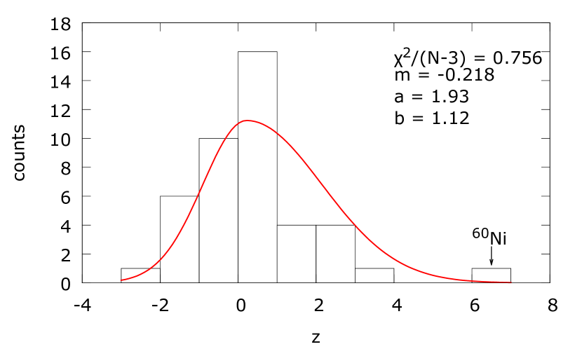
(a)

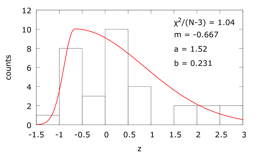
(b)

Figure 1: (a) Histograms of the $z$ values computed for the CE/DSAM method pair, together with the asymmetric normal distribution fit. The ⁶⁰Ni outlier in this dataset is also indicated. (b) Same as (a), but for the CE/($e,e^{\prime}$ ) pair.

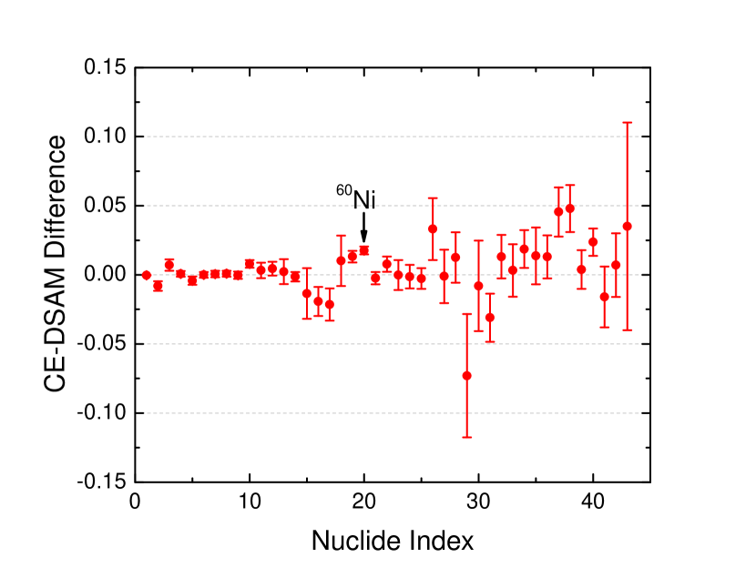
(a)

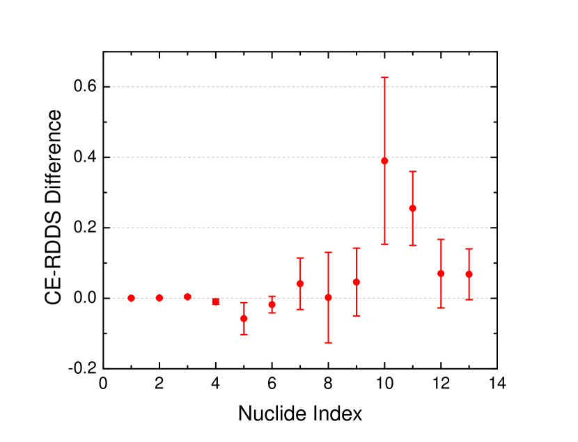
(b)

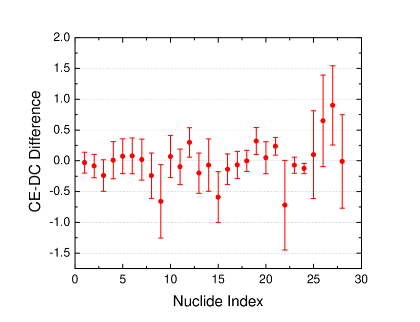
(c)

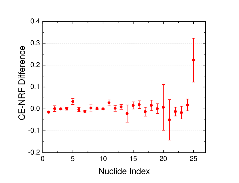
(d)

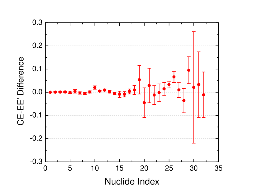
(e)

Figure 2: Difference between B(E2) values determined by CE and each other method: (a), (b), (c), (d) (e) compare with DSAM, RDDS, DC, NRF and ($e,e^{\prime}$ ) respectively. The x-axis in each plot shows the index associated with the nuclide for that pairing of methods. These indices are essentially arbitrary and differ between the different plots, but increasing index always corresponds to increasing mass number. See Table C1 to see which nuclide corresponds to each index.

In order to systematically establish the equivalence of each method to one another, we performed this analysis for each pair of methods and did not find any pairs which satisfied criteria (ii) or (iii), although a DSAM/CE and DSAM/NRF did satisfy (i). However, in both of these cases neither of the other two criteria are also satisfied. This gives some evidence that there may be problems with some of DSAM measurements, but not necessarily anything systematically wrong with the method itself. Indeed, if the DSAM measurements for ⁶⁰Ni are excluded then the discrepancy with CE and NRF no longer exists. This is discussed in detail in Section 4. In this global comparison, we also do not have any evidence for a systematic deviation of B(E2) values in Sn nuclides as suggested in the recent study [1].

Since CE is the most commonly used method, and presumably it suffers less from systematic errors such as stopping powers in DSAM method, detailed results for comparing CE with several other methods are shown in Table 1. Table 1 also further illustrates the asymmetry of the $z$-value distributions. For a symmetric distribution (i.e. usual normal distribution) $\mu_{d}=m$, yet in the table we see the mean and mode differ significantly in all cases. The comparison between CE and each of the other methods can also be seen graphically in Fig. 2 where the difference (not normalized to the size of the error bars, i.e. $(x-y)$ and not $z$) between the B(E2) values measured by CE and each of the other methods are plotted.

Table 1: Comparison between CE and five other methods using each of the metrics outlined in equations (3), (4) and (5) and used to define non-equivalence criteria (i)-(iii). The quantity $\chi^{2}/(N-3)$ gives the reduced $\chi^{2}$ values for the fit of an asymmetric normal distribution to the calculated $\{z_{i}\}_{i=1}^{N}$, establishing the goodness of fit.

Method	$\chi^{2}/(N-3)$	$P_{1}$	$\mu_{d}$	$m$
DSAM∗	0.756	0.513	0.428	$-0.218$
RDDS	0.491	0.423	0.484	0.697
DC	0.533	0.229	0.0156	$-0.220$
NRF	2.51	0.444	$-0.236$	0.116
$e,e^{\prime}$	1.04	0.256	0.362	$-0.667$

^∗ If the ⁶⁰Ni DSAM measurements are excluded then $P_{1}=0.469$, $\mu_{d}=0.264$, $m=0.0944$.

4 Discussion and Conclusion

The results of Table 1 overall indicate that each method used to measure B(E2) values is equivalent to CE, however some points are worth further discussion. All the $\chi^{2}/(N-3)$ values are smaller than the critical $\chi^{2}$ values for rejection at 99% confidence except NRF, i.e. only the CE/NRF normalized differences are not well-modelled by an asymmetric normal distribution. However, a visual inspection of Fig. 2(d) reveals that, even if the numeric values of the parameters for NRF in Table 1 are not meaningful, the conclusion of equivalence is still supported. Indeed, about 75% of the CE/NRF differences lie within one standard deviation of zero.

The only indication of non-equivalence in Table 1 is $P_{1}>0.5$ for CE/DSAM. Although not listed, it is also true that $P_{1}>0.5$ for NRF/DSAM as well. This could indicated a systematic problem with DSAM measurements, however the reason for these discrepancies can be attributed to measurements on a single nucleus, ⁶⁰Ni. As can be seen in the histogram of Fig. 1(a) a single $z$ value is separated from the bulk of the distribution by at least a full unit (standard deviation). This data point is also indicated in Fig. 2(a) and one can see that indeed the error bars are very small compared to its deviation from zero (hence the large value of $z$ for this measurement). This disagreement between CE and DSAM measurements was also noted in [8], although very good agreement was found for ⁶²Ni. Further evidence against the DSAM lifetime measurements of ⁶⁰Ni is the fact that they are in mutual disagreement with one another. The more recent measurements give $\sim$1.3 ps [9, 10] and earlier measurements $\sim$1 ps [11, 12]. This could be due to problems with one or more of the DSAM measurements of this nucleus as a result of poorly determined stopping powers, improperly implemented inverse kinematics during data analysis or ignored possible angular correlations. In any case, it appears that the ⁶⁰Ni DSAM measurements are an isolated problem rather than evidence of a broad systematic issue with the method. By excluding these measurements from the analysis, there is no longer significant evidence that DSAM disagrees with CE or NRF.

In conclusion, based on the analyses performed on the most recently compiled B(E2) experimental data [5], we conclude that the most commonly methods used in the measurement of B(E2) values are equivalent. There is some evidence to suggest that there is disagreement between DSAM and CE as well as DSAM and NRF methods, however these appear to arise from discrepant DSAM measurements in the lifetime of ⁶⁰Ni and not from a systematic deficiency in the method itself. Similarly, we do not find evidence for systematic deviation between DSAM and CE results for Sn nuclei, when all the available experimental data are considered. It is possible that DSAM results reported in [2] suffer from some experimental difficulties.

5 Acknowledgments

We are indebted to Dr. M. Herman (BNL) for support of this project. The authors gratefully acknowledge J.M. Allmond (ORNL) for providing his latest results and fruitful discussions. Work at Brookhaven was funded by the Office of Nuclear Physics, Office of Science of the U.S. Department of Energy, under Contract No. DE-AC02-98CH10886 with Brookhaven Science Associates, LC. Work at McMaster University was partially supported by the Office of Science of the U.S. Department of Energy.

Appendix A Table of Data

Table A1: B(E2) recalculated weighted averages for DSAM, RDDS, DC, CE, NRF and $e,e^{\prime}$ experimental methods using the relevant compiled data in Table 1 of 2016 compilation [5].

Nuclei	B(E2)$\uparrow$ ($e^{2}b^{2}$)
	DSAM	RDDS	DC	CE	NRF	$e,e^{\prime}$
12C	0.00400(20)				0.00334(71)	0.00399(33)
16O					0.00371(32)	0.00413(36)
18O	0.00458(24)	0.00405(20)		0.00429(15)		0.00449(22)
18Ne	0.0241(22)			0.0160(26)
20Ne	0.0299(28)			0.0369(30)
22Ne	0.0230(15)	0.0229(11)		0.0237(14)		0.0232(22)
24Mg	0.0472(23)	0.0391(19)		0.0430(20)	0.0578(32)	0.0421(23)
26Mg	0.0309(15)			0.0309(15)	0.030(13)	0.0298(21)
28Si	0.0323(16)			0.0329(17)	0.0330(27)	0.0348(31)
32S	0.0293(14)			0.0301(16)	0.0296(58)	0.0259(74)
34S	0.0210(12)			0.0207(24)
36Ar	0.0219(16)			0.0298(23)
40Ar	0.0327(24)			0.0359(50)
40Ca	0.0093(10)				0.0103(11)	0.00703(82)
42Ca	0.0334(24)				0.060(12)	0.0367(49)
44Ca	0.0440(36)			0.0485(35)		0.0517(35)
48Ca	0.0085(13)					0.00826(50)
46Ti		0.0995(48)		0.0898(60)	0.056(12)
48Ti	0.0626(55)			0.0649(72)	0.0676(60)
50Ti	0.0281(19)			0.0267(29)
50Cr	0.118(18)			0.1045(32)
52Cr	0.077(10)			0.0573(31)	0.0687(13)	0.0627(39)
54Fe	0.077(11)			0.0551(38)		0.0539(24)
56Fe	0.088(18)			0.0981(26)	0.094(14)	0.0777(67)
58Ni	0.0560(37)			0.0692(20)	0.0665(59)	0.0643(25)
60Ni	0.0750(21)			0.0926(20)	0.0927(20)	0.0832(37)
62Ni	0.0908(34)			0.0884(30)		0.0862(46)
64Ni	0.0590(40)			0.0668(38)		0.0720(41)
64Zn	0.1512(42)			0.151(10)	0.1237(93)	0.1601(90)
66Zn	0.1379(29)			0.1366(80)	0.134(11)	0.1454(80)
68Zn	0.1206(26)			0.1179(70)	0.1091(81)	0.1145(80)
70Zn	0.1429(80)			0.176(21)
70Ge	0.179(19)			0.1779(35)
72Ge	0.196(18)			0.2086(30)	0.230(39)
72Se	0.183(20)	0.190(15)
78Kr	0.674(33)	0.659(34)		0.601(30)
80Kr	0.396(26)			0.388(20)
86Sr	0.1400(70)			0.109(16)
88Sr	0.0909(47)			0.104(15)	0.0882(59)	0.094(12)
90Zr	0.086(13)					0.057(10)
92Mo	0.102(18)			0.1052(60)
94Mo	0.1959(95)			0.2145(98)
96Mo	0.269(15)			0.283(14)
96Ru	0.231(10)			0.244(12)
98Ru		0.413(14)		0.395(19)
106Pd				0.662(37)		0.608(49)
108Pd				0.762(50)		0.807(40)
110Pd		0.838(42)		0.879(60)		0.850(44)
110Cd				0.438(21)		0.450(35)
114Cd				0.536(25)		0.538(28)
112Sn	0.195(14)			0.241(11)
114Sn	0.185(12)			0.233(12)
116Sn				0.2135(50)	0.194(17)	0.199(27)
118Sn				0.2052(40)	0.218(20)	0.172(14)
120Sn	0.1982(98)			0.202(10)	0.186(22)	0.136(22)
124Sn	0.1414(90)			0.1651(41)	0.164(22)
122Te				0.647(30)	0.64(10)
124Te				0.566(28)	0.616(88)
124Xe		0.978(66)		0.98(11)
130Ba		1.111(55)		1.157(79)
138Ba				0.229(11)	0.241(17)
144Ba		1.02(18)	1.020(55)
140Ce	0.307(16)			0.291(15)	0.308(25)
142Ce				0.467(23)		0.457(23)
142Nd	0.265(13)			0.272(19)	0.254(19)	0.308(49)
146Nd				0.750(38)		0.655(44)
144Sm	0.228(74)			0.263(13)
152Sm			3.4613(23)	3.43(17)		3.41(17)
154Gd			3.874(16)	3.79(19)
156Gd			4.77(11)	4.53(23)
158Gd			5.08(17)	5.09(25)
160Gd			5.21(11)	5.28(26)
156Dy			3.66(22)	3.74(19)
158Dy			4.65(24)	4.67(23)
162Dy			5.27(26)	5.03(26)
162Er			5.61(54)	4.95(25)
164Er			5.25(21)	5.32(27)
166Er			5.78(16)	5.68(24)
168Er			5.681(59)	5.98(23)
172Yb			6.16(15)	5.96(29)
174Yb			5.91(31)	5.84(29)
174Hf			5.89(22)	5.30(35)
178Hf			4.797(94)	4.66(23)
180Hf			4.6471(30)	4.58(22)
182W			4.091(61)	4.09(16)
184W			3.57(11)	3.89(19)
186Os			3.060(72)	3.11(25)
188Os			2.449(59)	2.69(13)
190Os		1.98(21)	3.09(72)	2.37(11)
192Os				2.04(10)		2.01(10)
192Pt			2.002(95)	1.931(90)
194Pt		1.428(68)		1.683(80)
196Pt		1.348(70)		1.418(68)		1.429(71)
198Pt		1.030(52)		1.098(50)
198Hg			1.084(83)	0.9600(68)	0.74(10)
208Pb					0.263(18)	0.312(16)
230Th			8.12(21)	8.22(68)
234U			9.92(50)	10.57(55)
236U			10.78(28)	11.68(58)
240Pu			13.12(39)	13.11(65)

Appendix B Additional $z$-Value Histograms

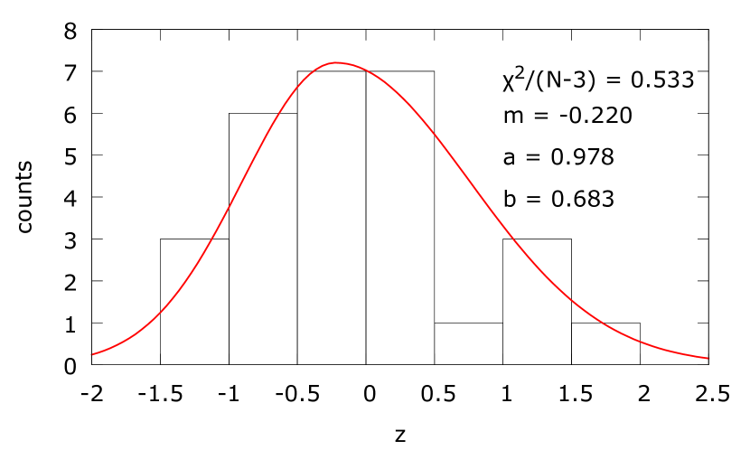
(a)

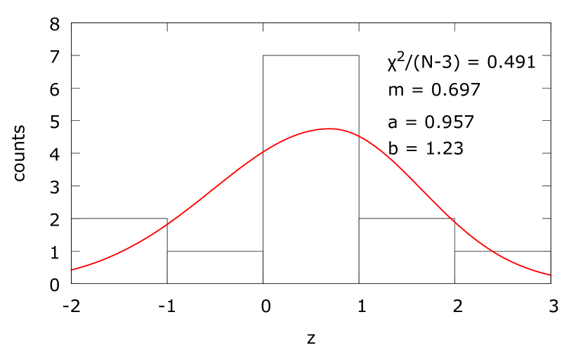
(b)

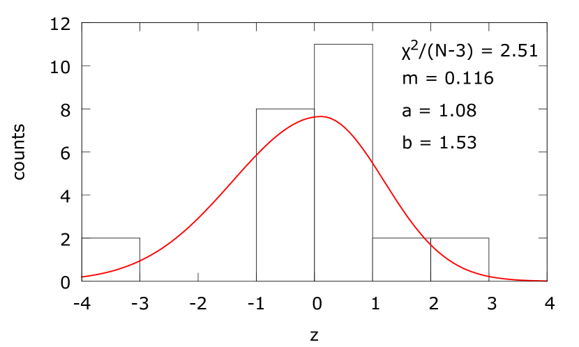
(c)

Figure B1: (a) Histograms of the $z$ values computed for the CE/DC method pair, together with the asymmetric normal distribution fit. (b) Same as (a), but for the CE/RDDS pair. (c) Same as (a), but for the CE/NRF pair.

Appendix C Nuclide Indices

Table C1: List of nuclides corresponding to the indices given on the x-axes of the plots in Fig. 2.

Index	Fig. 2(a)	Fig. 2(b)	Fig. 2(c)	Fig. 2(d)	Fig. 2(e)	Index	Fig. 2(a)
1	18O	18O	152Sm	24Mg	18O	33	92Mo
2	18Ne	22Ne	154Gd	26Mg	22Ne	34	94Mo
3	20Ne	24Mg	156Gd	28Si	24Mg	35	96Mo
4	22Ne	46Ti	158Gd	32S	26Mg	36	96Ru
5	24Mg	78Kr	160Gd	46Ti	28Si	37	112Sn
6	26Mg	98Ru	156Dy	48Ti	32S	38	114Sn
7	28Si	110Pd	158Dy	52Cr	44Ca	39	120Sn
8	32S	124Xe	162Dy	56Fe	52Cr	40	124Sn
9	34S	130Ba	162Er	58Ni	54Fe	41	140Ce
10	36Ar	190Os	164Er	60Ni	56Fe	42	142Nd
11	40Ar	194Pt	166Er	64Zn	58Ni	43	144Sm
12	44Ca	196Pt	168Er	66Zn	60Ni
13	48Ti	198Pt	172Yb	68Zn	62Ni
14	50Ti		174Yb	72Ge	64Ni
15	50Cr		174Hf	88Sr	64Zn
16	52Cr		178Hf	116Sn	66Zn
17	54Fe		180Hf	118Sn	68Zn
18	56Fe		182W	120Sn	88Sr
19	58Ni		184W	124Sn	106Pd
20	60Ni		186Os	122Te	108Pd
21	62Ni		188Os	124Te	110Pd
22	64Ni		190Os	138Ba	110Cd
23	64Zn		192Pt	140Ce	114Cd
24	66Zn		198Hg	142Nd	116Sn
25	68Zn		230Th	198Hg	118Sn
26	70Zn		234U		120Sn
27	70Ge		236U		142Ce
28	72Ge		240Pu		142Nd
29	78Kr				146Nd
30	80Kr				152Sm
31	86Sr				192Os
32	88Sr				196Pt

References

References

- [1] J.M. Allmond, A.E. Stuchbery, A. Galindo-Uribarri et al., Phys. Rev. C 92, (2015) 041303(R).
- [2] A. Jungclaus, J. Walker, J. Leske et al., Phys. Lett. B 695 (2011) 110.
- [3] J.M. Cook, T. Glasmacher, A. Gade, Phys. Rev. C 73 (2006) 024315.
- [4] H. Scheit, A. Gade, T. Glasmacher, T. Motobayashi, Phys. Lett. B 659 (2008) 515.
- [5] B. Pritychenko, M. Birch, B. Singh, M. Horoi, At. Data Nucl. Data Tables 107 (2016) 1.
- [6] S. Raman, C.W. Nestor, P. Tikkanen, At. Data Nucl. Data Tables 78 (2001) 1.
- [7] P. Royston, Appl. Stat. 44 (1995) 547.
- [8] J.M. Allmond, B.A. Brown, A.E. Stuchbery et al., Phys. Rev. C 90 (2014) 034309.
- [9] O. Kenn, K.-H. Speidel, R. Ernst et al., Phys. Rev. C 63 (2001) 021302.
- [10] J.N. Orce, B. Crider, S. Mukhopadhyay et al., Phys. Rev. C 77 (2008) 064301.
- [11] T.R. Fisher, P.D. Bond, Part. and Nucl. 6 (1973) 119.
- [12] H. Ronsin, P. Beuzit, J. Delaunay et al., Nucl. Phys. A 207 (1973) 557.