Cosmological Perturbations without Inflation

Abstract

A particularly attractive feature of inflation is that quantum fluctuations in the inflaton field may have seeded inhomogeneities in the cosmic microwave background (CMB) and the formation of large-scale structure. In this paper, we demonstrate that a scalar field with zero active mass, i.e., with an equation of state $\rho+3p=0$, where $\rho$ and $p$ are its energy density and pressure, respectively, could also have produced an essentially scale-free fluctuation spectrum, though without inflation. This alternative mechanism is based on the Hollands-Wald concept of a minimum wavelength for the emergence of quantum fluctuations into the semi-classical universe. A cosmology with zero active mass does not have a horizon problem, so it does not need inflation to solve this particular (non) issue. In this picture, the $1^{\circ}-10^{\circ}$ fluctuations in the CMB correspond almost exactly to the Planck length at the Planck time, firmly supporting the view that CMB observations may already be probing trans-Planckian physics.

1 Introduction

In spite of its many successes, standard big-bang cosmology suffers from several conceptual and physical anomalies and inexplicable observational puzzles, such as the ‘horizon’ problem, in which the cosmic microwave background (CMB) temperature is relatively uniform everywhere, even though causally connected regions at last scattering are much smaller than the horizon size today. Founded on a combination of classical and quantum physical principles [1, 2, 3], the inflationary paradigm was developed to address these issues [4, 5, 6, 7, 8]. But though the idea of inflation is very flexible, it has yet to find expression in a comprehensive, self-consistent model that accounts for all of the observations [9].

Many variations of the inflationary concept exist today [2, 3, 10, 11, 12, 13, 14, 15], allowing us to parametrize features in the early universe, but none may represent a final comprehensive answer if their fundamentally semi-classical nature is at odds with Planckian (or even pre-Planckian) scale physics. On the other hand, an inflationary phase may have been associated with a scalar (‘inflaton’) field beyond the Planck scale, whose identity could eventually be revealed via extensions to the Standard Model based on supergravity, grand unified theories, or even string theory.

Most of the problems arising in standard big-bang cosmology are due to the inevitable decelerated expansion associated with a radiation or matter dominated cosmic fluid. Inflation circumvents this deficiency by postulating the existence of an early phase of accelerated expansion, during which proper distances grew faster than the gravitational horizon size, which in some inflationary scenarios actually did not grow at all (or grew very slowly) during this brief period. Thus, physical distances would have been pushed beyond the Hubble radius, which potentially solves the horizon problem.

An additional attractive feature of inflation—central to the subject of this paper—is that quantum fluctuations of the inflaton field may have generated density perturbations seeding the formation of large-scale structure [16, 17, 18, 19]. These fluctuations would have been stretched on large scales by the brief accelerated expansion and, in the simplest version of the single inflaton field scenario, would have become ‘frozen’ after their wavelength exceeded the Hubble radius. And since inflation must have somehow ended in order for the Universe to subsequently re-establish its radiation and matter dominated expansion, the perturbations would have crossed back inside the Hubble radius.

In this picture, fluctuations with ever larger co-moving wavenumbers crossed the horizon and became frozen at progressively later times, a process naturally producing nearly scale-invariant spectra. This expectation has been largely confirmed by measurements of the temperature anisotropies in the CMB, generating considerable enthusiasm for the inflationary paradigm, well beyond its early success in apparently resolving other long-standing issues, such as the aforementioned horizon problem.

Even so, tension continues to grow between the overall expectations of the inflationary model and some key observations including, and especially, of the CMB anisotropies. The emergence of greater detail in all-sky maps has revealed several unexpected features on large scales, first reported by the Cosmic Background Explorer (COBE) Differential Microwave Radiometer (DMR) collaboration [20]. Disagreement with theory arises from an apparent alignment of the largest modes of CMB anisotropy, as well as the absence of any angular correlation at angles greater than $\sim 60^{\circ}$. The latter is particularly troublesome because all fluctuations presumably exited the horizon during inflation, which should have produced a correlation at all angles. These unexpected features have been explained as possibly due to cosmic variance within the standard model [21], but this explanation may not be completely satisfactory.

An analysis of the differences between the observed angular correlation function and that predicted by inflation in $\Lambda$CDM [22] has revealed that only $\sim 0.03\%$ of $\Lambda$CDM model CMB skies have a variance larger than that of the sky observed with the Wilkinson Microwave Anisotropy Probe (WMAP) [21]. We may simply be dealing with foreground subtraction issues. But there are indications that the differences between theory and observations may be due to more than just randomness. For example, the well-defined shape of the observed angular correlation function, with a minimum at $\sim 50^{\circ}$, is at odds with the expectation that the data points would not have lined up as they do within the variance window if stochastic processes were solely to blame. More importantly, the observed angular correlation goes to zero beyond $\sim 60^{\circ}$. While variance could have resulted in a function with a different slope than that predicted by inflation, it seems unlikely that this randomly generated slope would be close to zero above $\sim 60^{\circ}$.

This tension has been exacerbated by the more recent Planck results [23]. The probability of the Planck sky being consistent with inflation in $\Lambda$CDM is $\sim 0.33\%$ for any of the analyzed combinations of maps and masks [24], a trend that has now remained intact through three different satellite missions (COBE, WMAP, Planck). The apparent lack of temperature correlations at large angles is robust and increases in statistical significance as the quality of the measurements improves, suggesting that instrumental issues are not the cause. Indeed, if it turns out that the absence of large-angle correlation is real, this may be the most significant outcome of the CMB observations, because it would essentially invalidate any role that inflation might have played in the universal expansion.

In this paper, we consider an alternative scenario for generating quantum fluctuations in the early universe, not solely because of the potential problems facing inflation in accounting for all the data, but more so because another Friedmann-Robertson-Walker (FRW) cosmology, known as the $R_{\rm h}=ct$ universe [25, 26] (see also Ref. [27] for a non-technical introduction) has been shown in recent years to account for a broad range of high-precision cosmological measurements better (in some cases, significantly better) than $\Lambda$CDM, the current standard model based on inflation.

For example, whereas the inflationary paradigm has trouble explaining the absence of any angular correlation in the CMB beyond $\sim 60^{\circ}$, this characteristic simply results from the size of the gravitational horizon (i.e., the Hubble radius) at last scattering in the $R_{\rm h}=ct$ universe [28]. A rather compelling example of how the predictions of $\Lambda$CDM and $R_{\rm h}=ct$ differ in their comparisons with the data is provided by a recent application of the Alcock-Paczyński test [29], based on the changing ratio of angular to spatial/redshift size of (presumed) spherically-symmetric source distributions with distance, to the most accurate measurements of the baryon acoustic oscillation (BAO) scale. The use of this diagnostic with newly acquired data on the anisotropic distribution of the BAO peaks from SDSS-III/BOSS-DR11 at average redshifts $\langle z\rangle=0.57$ [30] and $\langle z\rangle=2.34$ [31], disfavors the current concordance ($\Lambda$CDM) model at better than a $99.34\%$ CL, while the probability that the $R_{\rm h}=ct$ universe is consistent with these data is $\sim 0.96$, i.e., essentially one [32].

The question concerning how quantum fluctuations were generated in the early universe is critical to this whole discussion because, whereas $\Lambda$CDM probably cannot survive without inflation, the $R_{\rm h}=ct$ universe does not have or need it. This cosmology did not undergo a period of decelerated expansion, and therefore avoids the horizon problem altogether [33]. So while this paper is in principle motivated separately by (1) a desire to alleviate the growing tension between the predictions of inflation and the ever improving observations, and (2) a need to strengthen the viability of the $R_{\rm h}=ct$ universe by uncovering a mechanism to generate cosmological perturbations in this model, in reality these two goals overlap considerably. Our principal task is to determine how and why quantum fluctuations could have grown in $R_{\rm h}=ct$ without inflation.

Before we begin our development of this mechanism, however, it is worthwhile considering several earlier attempts at producing quantum fluctuations without inflation, and how they differ from the proposal we are making here. In their work, Bengochea et al. [34] adopted the Hollands-Wand concept, but focused primarily on the question of how classicalization may actually occur in such a scenario. This issue, of how a homogeneous and isotropic quantum fluctuation is converted into actual inhomogeneities and anisotropies at the classical scale, is common to all models invoking a quantum origin for the perturbations, and is yet to be resolved (see also ref. [35]). In their analysis, these authors adopted a standard cosmological background (other than inflation), whereas in this paper we will focus exclusively on the zero active mass equation-of-state associated with the $R_{\rm h}=ct$ model. The manner in which the modes are born and subsequently stretch and grow is quite different in these two cases. As we shall see, the mode wavelength grows as a constant fraction of the Hubble radius, so its transition from the Planck domain to the $\sim 1^{\circ}-10^{\circ}$ scale associated with the CMB is smooth and does not involve multiple steps, such as one encounters during inflation, where modes cross and re-cross the horizon during their evolution. Nonetheless, this paper will not be fully addressing the question of classicalization, which remains a largely unresolved problem.

A non-inflationary mechanism for generating the perturbation spectrum has also been considered in ekpyrotic [36] and cyclic [37] models. Here too, however, these models have the common feature that the perturbations originated as quantum fluctuations which exited and re-entered the horizon during their evolution. Interestingly, this process occurs for both expanding cosmologies (e.g., in the standard model) and a contracting universe, with an appropriate alteration to the evolution in the scale factor $a(t)$ [38]. The cyclic model repeats its periods of expansion and contraction, the latter of which is identical to the ekpyrotic case. The $R_{\rm h}=ct$ model that we focus on in this paper is unique, in that this is the only case in which all proper distances and the Hubble radius expand at the same rate. As we shall see, the mechanism for producing a near-scale free spectrum is therefore simpler, with the added advantage that the observed scale of fluctuations in the CMB traces back directly to the Planck wavelength at the Planck time. None of the other models have this feature, which provides some justification for the argument that perturbations were essentially trans-Plancking in nature.

In § II of this paper, we briefly summarize the origin and essential characteristics of the $R_{\rm h}=ct$ universe, and then discuss the cosmological dynamics in this model in § III. The cosmological perturbations are introduced in § IV, where we describe some of this model’s most significant predictions. We end with our conclusions in § V.

2 The $R_{\rm h}=ct$ Universe

The $R_{\rm h}=ct$ universe is an FRW cosmology in which the underlying symmetries of the metric, with particular reference to Weyl’s postulate [39], are used to incorporate the influence of a gravitational horizon on the expansion dynamics [25, 26, 40]. The model is based on standard general relativity (GR), and the Cosmological principle is adopted from the start, just like any other FRW cosmology, but it equally addresses the consequences of Weyl’s postulate, whose role in shaping the FRW metric is often ignored.

It is commonly assumed that Weyl’s postulate is already incorporated into all forms of the FRW metric, and is therefore given far less attention than the Cosmological principle. Simply stated, Weyl’s postulate holds that any proper distance $R(t)$ is a product of a universal expansion factor $a(t)$ (dependent only on cosmic time $t$) and an unchanging co-moving radius $r$: $R(t)=a(t)r$. We conventionally write the FRW metric adopting this coordinate definition, along with $t$, which is actually the observer’s proper time in his/her free-falling frame.

But its impact is far greater than this. Consider, for instance, the Misner-Sharp mass $M$—defined in terms of the proper mass density $\rho/c^{2}$ and proper volume $4\pi R^{3}/3$ [41]—in this spacetime. In terms of the proper mass $M$, the gravitational radius of the Universe is $R_{\rm h}\equiv 2GM/c^{2}$ [25, 40], which actually coincides with the better known Hubble radius $c/H(t)$. Given its definition, $R_{\rm h}$ (and therefore the Hubble radius) is a proper distance [40], so this radius must comply with Weyl’s postulate, the consequence of which is the unique choice $a(t)=(t/t_{0})$ for the expansion factor, where $t_{0}$ is the current age of the Universe [26]. Those familiar with the properties of the Schwarzschild or Kerr metrics are not at all surprised by this constraint, which leads to the result that the gravitational radius must be receding from us at speed $c$—hence the name ‘$R_{\rm h}=ct$’ for this model. The Hubble radius was in fact defined to be the distance at which the Hubble speed equals $c$ even before it was recognized as another manifestation of the gravitational horizon. In black-hole spacetimes, a free-falling observer sees the event horizon approaching them at speed $c$, so this property of $R_{\rm h}=ct$ is quite familiar in the context of standard GR.

One of the principal differences between $R_{\rm h}=ct$ and other FRW cosmologies, such as $\Lambda$CDM, is how they handle the energy density $\rho$ and pressure $p$, and their temporal evolution. In $\Lambda$CDM we routinely start with the constituents in the cosmic fluid, and assume their equations-of-state, and then solve the dynamics equations to determine the expansion rate as a function of time. In $R_{\rm h}=ct$, on the other hand, the symmetries of the FRW metric and the properties of the gravitational horizon, uniquely specify the spacetime curvature, and hence the expansion rate, strictly from just the value of the total energy density $\rho$, without us having to know the specifics of the constituents themselves. In this model, the constituents of the Universe must partition themselves in such a way as to satisfy the constant expansion rate required by the $R_{\rm h}=ct$ condition. Insofar as the dynamics is concerned, all that matters is $\rho$ and the overall equation of state $p\equiv w\rho$. So while one assumes $\rho=\rho_{m}+\rho_{r}+\rho_{\Lambda}$ in $\Lambda$CDM, i.e., that the principal constituents are matter, radiation, and a cosmological constant $\Lambda$, and then infers $w$ from the equations-of-state assigned to them, in $R_{\rm h}=ct$, it is the aforementioned symmetries and other constraints from GR that force the $R_{\rm h}=ct$ universe to have the unique equation-of-state [25, 26]

$$\rho+3p=0\;.$$ (1)

The $R_{\rm h}=ct$ cosmology is therefore simple and elegant, in the sense that observable quantities, such as the luminosity distance $d_{L}$ and the redshift dependence of the Hubble constant $H$, take on analytic forms:

$$d_{L}=R_{h}(t_{0})(1+z)\ln(1+z)\;,$$ (2)

and

$$H(z)=H_{0}(1+z)\;,$$ (3)

where $z$ is the redshift, $R_{h}(t)=c/H(t)$, and $H_{0}$ is the value of the Hubble constant today. Relations such as these have been tested using a broad range of measurements, such as the BAO observations described above, and have thus far accounted for the data better than their counterparts in $\Lambda$CDM [28, 42, 43, 44, 45, 46, 47, 48, 49, 51, 50, 52, 53, 54, 55, 56].

Nonetheless, with its empirical approach, $\Lambda$CDM has done remarkably well as a reasonable approximation to $R_{\rm h}=ct$ in restricted redshift ranges. For example, using the ansatz $\rho=\rho_{m}+\rho_{r}+\rho_{\Lambda}$ to fit the data, one finds that the parameters in the standard model must have quite specific values, such as $\Omega_{m}\equiv\rho_{m}/\rho_{c}\sim 0.27$, where $\rho_{c}$ is the critical density [57]. However, with these parameters, $\Lambda$CDM then requires $R_{\rm h}(t_{0})\approx ct_{0}$ today, which is in fact the baseline constraint in the $R_{\rm h}=ct$ model. One concludes from this that the optimized $\Lambda$CDM cosmology describes a universal expansion equal to what it would have been with $R_{\rm h}=ct$ all along. And many other indicators support the view that using $\Lambda$CDM to fit the data therefore produces a cosmology almost, but not entirely identical, to $R_{\rm h}=ct$, in spite of the fact that with its many free parameters, $\Lambda$CDM could have had an entirely diverse set of expansion histories.

3 Cosmological Dynamics

3.1 Field Equations

The Friedmann-Robertson-Walker metric is conventionally written in terms of the comoving coordinates $(t,r,\theta,\phi)$, and takes the form

$$ds^{2}=dt^{2}-a(t)^{2}\left[{dr^{2}\over 1-Kr^{2}}+r^{2}\left(d\theta^{2}+\sin^{2}\theta\,d\phi^{2}\right)\right]\;,$$ (4)

where $K$ is the spatial curvature constant. In $R_{\rm h}=ct$, $K$ must be zero in order for the gravitational radius to coincide with the Hubble radius, which the data (interpreted in the context of $\Lambda$CDM) all seem to be confirming as well. We will therefore henceforth set $K=0$ in all our derivations.

The dynamical equations for this background FRW metric are obtained from Einstein’s equations,

$$G_{\alpha\beta}\equiv\mathcal{R}_{\alpha\beta}-{1\over 2}g_{\alpha\beta}\mathcal{R}=-{8\pi G}T_{\alpha\beta}\;,$$ (5)

where $g_{\alpha\beta}$ are the metric coefficients, and $\mathcal{R}_{\alpha\beta}$ and $\mathcal{R}$ are the Ricci tensor and scalar, respectively:

$$H^{2}\equiv\left({\dot{a}\over a}\right)^{2}={8\pi G\over 3}\rho\;,$$ (6)

and

$${\ddot{a}\over a}=-{4\pi G\over 3}\left(\rho+3p\right)\;,$$ (7)

where a dot denotes a derivative with respect to $t$, and $\rho$ and $p$ are, of course, the proper energy density and pressure in the co-moving frame. Throughout this paper, we work with natural units, in which $\hbar=c=1$. The continuity equation for the (perfect fluid) energy-momentum tensor,

$$T_{\alpha\beta}=\left(\rho+p\right)u_{\alpha}u_{\beta}-pg_{\alpha\beta}\;,$$ (8)

in terms of the four-velocity $u_{\alpha}$, yields a third (though not independent) equation, expressing the (local) conservation of energy:

$$\dot{\rho}=-3H(\rho+p)\;.$$ (9)

3.2 The Numen Field

In the inflationary model, one assumes the existence of scalar inflaton fields that dominate $\rho$ in the cosmic fluid prior to the onset of leptogenesis and baryogenesis, with properties that lead to an exponential solution for $a(t)$ in Equations (6) and (7), thus heralding a very brief period of de Sitter expansion [58]. It is not difficult to imagine such fields influencing cosmological dynamics in the very early universe. For example, a grand unified theory based on the group SO(10) implies the existence of $\sim 100$ Higgs fields, and supersymmetry relies on the existence of many superpartners [59]. In addition, string theory has dynamical moduli fields associated with the geometrical characteristics of compactified dimensions [60].

Though the $R_{\rm h}=ct$ universe does not need or have inflation, and therefore does not require the presence of an ‘inflaton’ field, we will nonetheless assume that at least one scalar field dominated the cosmological dynamics at the very beginning. But unlike the situation with the standard model, the expansion factor $a(t)$ in the $R_{\rm h}=ct$ universe must always be proportional to $t$, so the expansion in this cosmology is never inflated. To clearly distinguish the hypothesized scalar field $\phi$ associated with the expansion in this model from those generally categorized as ‘inflaton’ fields, we will therefore refer to it informally as the ‘numen’ field, giving rise to the earliest manifestation of substance in the nascent universe, with an equation-of-state $\rho_{\phi}+3p_{\phi}=0$ and, as we shall see very shortly, whose quantum fluctuations might have seeded the subsequent formation of large-scale structure.

A crucial difference between the $R_{\rm h}=ct$ universe and other FRW cosmologies is that the cosmic fluid in the former has strictly ‘zero active mass,’ meaning that $\rho+3p=0$, so the expansion proceeds without any net gravitational influence (after all, this is why $\dot{a}$=constant). This suggests that coupling the numen field non-minimally to gravity using the simple prescription $\xi\mathcal{R}\phi^{2}/2$ [65, 66] (where $\xi$ is a dimensionless coupling constant) in the Lagrangian density may not be as relevant here as it is in the inflaton case (though not impossible, of course). We will rely on the simplest assumption we can make, i.e., that the background dynamics is dominated by a single homogeneous minimally-coupled scalar field with action

$$S=\int d^{4}x\sqrt{-g}\;\mathcal{L}(\phi,\partial_{\mu}\phi)\;,$$ (10)

where $\sqrt{-g}=a^{3}(t)$ for the metric in Equation (4), and the Lagrangian density is given as

$$\mathcal{L}={m_{\rm P}^{2}\over 16\pi}\mathcal{R}+{1\over 2}\partial^{\mu}\phi\partial_{\mu}\phi-V(\phi)\;,$$ (11)

where $m_{\rm P}\equiv G^{-1/2}$ is the Planck mass. As it turns out, the potential $V(\phi)$ for the numen field $\phi$ is unique in $R_{\rm h}=ct$, and we shall derive it very shortly.

Since the (background) field is homogeneous, we can ignore spatial gradients, and so the corresponding energy density $\rho_{\phi}$ ($=T_{00}$) and pressure $p_{\phi}$ ($=T_{ii}$) are given simply as

$$\rho_{\phi}={1\over 2}{\dot{\phi}}^{2}+V(\phi)\;,$$ (12)

and

$$p_{\phi}={1\over 2}{\dot{\phi}}^{2}-V(\phi)\;.$$ (13)

The zero active mass condition therefore immediately constrains the potential to have the unique form

$$V(\phi)={{\dot{\phi}}^{2}}\;,$$ (14)

and the energy conservation Equation (9) gives

$$\ddot{\phi}+3H\dot{\phi}+{\partial V\over\partial\phi}=0\;,$$ (15)

the usual Klein-Gordon equation.

The Friedmann Equation (6) similarly reduces to a very simple form,

$$H^{2}={4\pi\over m_{\rm P}^{2}}V(\phi)\;,$$ (16)

and combining this with Equation (14) then allows us to find an exact solution for the numen field:

$$\phi(t)-\phi(t_{i})={m_{\rm P}\over\sqrt{4\pi}}\ln\left({t\over t_{i}}\right)\;,$$ (17)

where $t_{i}$ is some fiducial time at which the field has an amplitude $\phi(t_{i})$. Returning to Equation (14), we therefore also have an exact—and unique—solution for the numen potential:

$$V(\phi)=V_{0}\,\exp\left\{-{2\sqrt{4\pi}\over m_{\rm P}}\,\phi\right\}$$ (18)

where, for convenience, we have defined the constant

$$V_{0}\equiv{m_{\rm P}^{2}\over 4\pi\,t_{i}^{2}}\exp\left\{{2\sqrt{4\pi}\over m_{\rm P}}\phi(t_{i})\right\}\;.$$ (19)

It is interesting to note that before settling on de Sitter (or quasi de Sitter) expansion for the inflationary paradigm, there were attempts in the 1980’s to consider minimally coupled inflaton fields with an exponential potential

$$V_{p}(\phi)=V_{0}\,\exp\bigg{\{}\pm{2\over p}{\sqrt{4\pi}\over m_{\rm P}}\,\phi\bigg{\}}\;,$$ (20)

as a means of producing so-called power-law inflation (PLI) with $p>1$ [61, 62, 63, 64]. During PLI, the scale factor has the time dependence

$$a(t)\propto t^{p}\;.$$ (21)

Again, the intention with these was to circumvent the problems arising from deceleration in standard big bang cosmology. The numen-field potential (Equation 18) is clearly a special member of this class, though with $p=1$ it does not inflate. Exponential potentials such as these are generally motivated in the context of Kaluza-Klein cosmologies [62], and arise in string theories, supergravity, and actually any theory based on a conformal transformation to the Einstein frame.

A difficulty commonly encountered with inflaton models is that they lack an exit mechanism for a decelerating (radiation or matter dominated) phase to succeed inflation. In contrast, the expansion rate is always constant in $R_{\rm h}=ct$, so no dynamical transition is required as the numen field decays into radiation and other particles in the standard model (via channels yet to be determined).

4 Cosmological Perturbations

We have learned from inflationary cosmology that to properly interpret anisotropies in the CMB, one needs a description of the fluctuations characterized by several observables. These include: (1) the scalar spectral index $n_{s}$, (2) the spectral index $n_{T}$ of the tensor perturbations and (where possible) (3) the tensor-to-scalar ratio $r$, giving the ratio of tensor to scalar amplitudes [67, 68]. The Wilkinson Microwave Anisotropy Probe (WMAP) [21] and Planck [23] have placed strong bounds on at least some of these parameters: $n_{s}=0.968\pm 0.006$ (corresponding to essentially a scale-free spectrum) and $r<0.11$ at $95\%$ CL.

Let us now consider small perturbations about the homogeneous numen field $\phi_{0}(t)$,

$$\phi(t,\vec{x})=\phi_{0}(t)+\delta\phi(t,\vec{x})\;,$$ (22)

keeping only terms to first order in $\delta\phi$. The inhomogeneity implied by these fluctuations requires that we also include metric perturbations about the spatially flat FRW background metric, which can be conveniently split into scalar, vector, and tensor components, depending on how they transform on spatial hypersurfaces.

By now, it is well known that vector perturbations have no lasting influence for scalar fields. The perturbed FRW spacetime for the remaining linearized scalar and tensor fluctuations is therefore described by the line element [12, 69, 70, 71]

$$ds^{2} = (1+2A)\,dt^{2}-2a(t)(\partial_{i}B)\,dt\,dx^{i}-$$ (23)

$$a^{2}(t)\left[(1-2\psi)\delta_{ij}+2(\partial_{i}\partial_{j}E)+h_{ij}\right]\,dx^{i}\,dx^{j}\,,\quad$$

where indices $i$ and $j$ denote spatial coordinates, and $A$, $B$, $\psi$ and $E$ describe the scalar degree of metric perturbations, while $h_{ij}$ represent the tensor perturbations. This form follows the notation of Ref. [71], aside from the use of the symbol $A$ instead of $\phi$ inside the lapse function (since we are reserving this symbol to represent the scalar field in this paper).

The Einstein equations for the scalar and tensor parts decouple to linear order, but the form of the scalar equation is gauge dependent. However, one can identify a variety of gauge-independent combinations of the scalar perturbations from within certain coordinate systems. For example, in the comoving frame, the curvature perturbation $\Theta$ on hypersurfaces orthogonal to comoving worldlines may be defined [69] as a gauge invariant combination of the metric perturbation $\psi$ and the scalar field perturbation $\delta\phi$:

$$\Theta\equiv\psi+\left({H\over\dot{\phi}}\right)\,\delta\phi\;.$$ (24)

4.1 Scalar Perturbations

Expanding $\Theta$ in Fourier modes,

$$\Theta(t,\vec{x})=\int{d^{3}\vec{k}\over(2\pi)^{3/2}}\,\Theta_{k}(t)e^{i\vec{k}\cdot\vec{x}}\;,$$ (25)

where $k$ is the comoving wavenumber, and using the linearized version of Einstein’s Equations (5) with the linearized metric in Equation (23), one arrives at the perturbed equation of motion

$$\Theta_{k}^{\prime\prime}+2\left({z^{\prime}\over z}\right)\Theta_{k}^{\prime}+k^{2}\Theta_{k}=0\;,$$ (26)

where overprime now denotes a derivative with respect to conformal time $d\tau\equiv{dt/a(t)}$. In the $R_{\rm h}=ct$ universe, we have $a(t)=(t/t_{0})$, where $t_{0}$ is a fixed time usually taken to be the present age of the Universe, so that $a(t_{0})=1$. Therefore

$$\tau(t)=\tau_{i}+t_{0}\ln\left({t\over t_{i}}\right)\;,$$ (27)

where $\tau_{i}$ is the conformal time at some fiducial cosmic time $t_{i}$. To simplify the notation, we will define the zero of conformal time to be at $t_{0}$, so throughout this paper we will employ the relation

$$\tau(t)=t_{0}\ln a(t)\;.$$ (28)

The quantity $z$ in Equation (26) is defined by the expression

$$z\equiv{a(t)(\rho_{\phi}+p_{\phi})^{1/2}\over H}\;.$$ (29)

Using Equations (6), (12) and (13) for the numen field, $z$ reduces to the much simpler form

$$z={m_{\rm P}\over\sqrt{4\pi}}a(t)\;,$$ (30)

and so $z^{\prime}/z=1/t_{0}$ and $z^{\prime\prime}/z=1/t_{0}^{2}$.

The quantity $z^{\prime}/z$ typically depends on the background dynamics, so one often conveniently rewrites Equation (26) in terms of the so-called Mukhanov-Sasaki variable $u_{k}\equiv z\,\Theta_{k}$ [72, 73]. It is not really necessary to do this here since $z^{\prime}/z$ and $z^{\prime\prime}/z$ are actually constant for the numen field, but we will take this step anyway just to make it easier to directly compare the differences between our solution and that pertaining to conventional inflaton fields. With this change of variable, the equation governing the curvature perturbation now becomes

$$u_{k}^{\prime\prime}+\alpha_{k}^{2}u_{k}=0\;,$$ (31)

where

$$\alpha_{k}\equiv{1\over t_{0}}\sqrt{\left(2\pi R_{\rm h}\over\lambda_{k}\right)^{2}-1}={1\over t_{0}}\sqrt{\left(kR_{\rm h}\over a\right)^{2}-1}\;,$$ (32)

and $\lambda_{k}\equiv 2\pi a/k$ is the proper wavelength corresponding to comoving wavenumber $k$.

This expression for the ‘frequency’ $\alpha_{k}$ is critical to understanding the nature of quantum fluctuations in the numen field. Its most distinct departure from inflaton fields is that both the gravitational radius $R_{\rm h}=t$, and the proper wavelength $\lambda_{k}\sim a(t)$, scale with time in exactly the same way, so the ratio $R_{\rm h}/\lambda_{k}$ or, equivalently, $kR_{\rm h}/a$, is constant. In this cosmology there is no crossing of wave modes back and forth across the horizon. In fact, once the wavelength of a mode is established when it emerges into the semi-classical universe, it remains a fixed fraction of the Hubble radius while both expand with time. And notice that all modes $u_{k}$ with a wavelength smaller than the horizon, $R_{\rm h}>\lambda_{k}/2\pi$, oscillate, while those with a super-horizon wavelength do not. (In this particular regard, the numen and inflaton fields behave similarly.) The analytic solution to Equation (31) may be written as follows:

$$u_{k}(\tau)=\left\{\begin{array}[]{ll}B(k)\,e^{\pm i\alpha_{k}\tau}&\mbox{($2\pi R_{\rm h}>\lambda_{k}$)}\\ B(k)\,e^{\pm|\alpha_{k}|\tau}&\mbox{($2\pi R_{\rm h}<\lambda_{k}$)}\end{array}\right.$$ (33)

The amplitude $B(k)$ is fixed by an appropriate choice of vacuum, related to how these modes are “born.” Quantum fluctuations of the inflaton field are created with a wavelength much smaller than the horizon, so they behave at first like an ordinary harmonic oscillator (similar to the oscillatory solution in Equation 33). But during inflation, $H$ is essentially constant, so $\lambda_{k}$ overtakes the Hubble radius $R_{\rm h}=1/H$ and becomes much larger, and the mode becomes an overdamped oscillator, with an amplitude that approaches a constant value, a process often referred to as “freezing.” Once inflation has ended, the Hubble radius resumes its rate of growth and overtakes $\lambda_{k}$, which is said to then “re-enter” the horizon.

In a time-independent spacetime, a preferred set of mode functions, and therefore an unambiguous physical vacuum, may be defined by minimizing the expectation value of the Hamiltonian. In Minkowski space, this means taking the positive frequency mode $u_{k}\sim e^{-ick\tau}$, i.e., the minimal excitation state, and setting $B(k)=1/\sqrt{2k}$ [12]. This prescription, however, does not usually generalize straightforwardly to time-dependent spacetimes, but this vacuum ambiguity can still be resolved in inflationary models by arguing that in the remote past all observable modes had a wavelength much smaller than the horizon, and were therefore not affected by gravity, so their frequencies were essentially time-independent. They therefore behaved as they would in Minkowski space. This approach defines the preferred set of mode functions and a unique physical vacuum known as the Bunch-Davies vacuum [74]. The amplitude $B(k)$ for super-horizon modes is then evaluated from the Bunch-Davies normalization by equating the amplitudes before and after freezing. And because the value of $a(t)$ at which the freezing occurs is proportional to $k$ (via the condition $k/a\sim 1/R_{\rm h}$), this process results in a scale-free spectrum (see below), consistent with the observed anisotropies in the CMB, considered to be one of the strongest factors in favor of the inflationary paradigm.

However, some have questioned the fundamental basis for this picture because in many models of inflation, the de Sitter phase lasted so long that the inflaton modes responsible for the creation of large-scale structure would have been born with wavelengths much shorter than the Planck scale (and therefore well before the Planck time), where the use of semi-classical physics is uncertain. This “trans-Planckian issue” [75] revolves around the question of whether the semi-classical description of our Universe breaks down prior to the Planck time, set by the condition that the Compton wavelength $\lambda_{\rm C}\equiv 2\pi/m$ of a mass $m$ be equal to its Schwarzschild radius $R_{\rm h}\equiv 2Gm$. Current physics may have to be modified on spatial scales smaller than the resulting Planck length $\lambda_{\rm P}\equiv\lambda_{\rm C}(m)$ at the specific value of $m$ where this equality is reached:

$$\lambda_{\rm P}=\sqrt{4\pi G}\;.$$ (34)

The corresponding Planck time $t_{\rm P}$ is simply this Planck length divided by the speed of light $c$. Numerically, we have $\lambda_{\rm P}\approx 5.7\times 10^{-33}$ cm and $t_{\rm P}\approx 1.9\times 10^{-43}$ s. These definitions actually make more sense for the $R_{\rm h}=ct$ universe than they do for the standard inflationary model, because the gravitational radius $R_{\rm h}$ is in fact equal to $t$, so the Planck time is simply the age of the Universe when the Hubble radius equaled the Planck scale (i.e., $R_{\rm h}=\lambda_{\rm P}$).

Let us now track the mode growth associated with the CMB anisotropies in the $R_{\rm h}=ct$ universe back to these earlier times and see how they are related to $\lambda_{\rm P}$ and $t_{\rm P}$ in this cosmology. The CMB spectrum has features ranging from sub-degree scales to tens of degrees. The Sachs-Wolfe effect [76], responsible for coupling the metric fluctuations with the primordial perturbations, contributes to temperature anisotropies on all scales, but tends to dominate at angles $\gtrsim 1^{\circ}-10^{\circ}$. On sub-degree scales, the spectral peaks are primarily dependent on the pressure and density variations associated with baryon acoustic oscillations. The characteristic CMB scale representing the effects of scalar/metric fluctuations therefore appears to be $\sim 1^{\circ}-10^{\circ}$.

In the $R_{\rm h}=ct$ cosmology, the angular-diameter distance is given as [25, 26, 50]

$$d_{A}={R_{\rm h}(t_{0})\over(1+z)}\ln(1+z)\;.$$ (35)

Therefore, a $\theta$-fluctuation at redshift $z_{\rm CMB}$ corresponds to a proper wavelength

$$\lambda^{\theta}(z_{\rm CMB})=2\pi\left({\theta\over 360^{\circ}}\right){R_{\rm h}(t_{0})\over(1+z_{\rm CMB})}\ln(1+z_{\rm CMB})\;.$$ (36)

And with $a(t)=t/t_{0}$, it is straightforward to see that at the Planck redshift, $z_{\rm P}\equiv t_{0}/t_{\rm P}-1$, the numen-field mode responsible for this anisotropy had a corresponding wavelength $\lambda^{\theta}(z_{\rm P})$ given by the expression

$${\lambda^{\theta}(z_{\rm P})\over\lambda_{\rm P}}\approx\left({\theta\over 57^{\circ}}\right)\ln(1+z_{\rm CMB})\;.$$ (37)

A precise estimate for $z_{\rm CMB}$ does not exist yet for the $R_{\rm h}=ct$ universe, but this uncertainty has negligible impact on the use of Equation (37) because the behavior of $d_{A}$ with redshift in this cosmology renders $\lambda^{\theta}(z_{\rm P})/\lambda_{\rm P}$ only weakly dependent on the redshift at last scattering. This may be seen in Table 1, where we quote the ratio $\lambda^{\theta}(z_{\rm P})/\lambda_{\rm P}$ for two angles ($\theta=1^{\circ}$ and $10^{\circ}$) and a very broad range of CMB redshifts. Clearly, the numen-field fluctuations producing the CMB anisotropies had a size comparable to the Planck scale were we to trace them back to the Planck time. The significance of this feature should not be underestimated. In the $R_{\rm h}=ct$ cosmology, the Universe underwent an expansion by over $60$ orders of magnitude in $a(t)$ between $z_{\rm P}$ and $z_{\rm CMB}$. Yet in this model the observed scale characterizing the CMB anisotropies tracks back directly to the Planck length at $t_{\rm P}$, in contrast to standard inflationary cosmology in which the CMB fluctuations have no obvious connection to the Planck scale. It would be a remarkable coincidence for $\lambda^{10^{\circ}}(z_{\rm P})\sim\lambda_{\rm P}$ if these two scales were not related dynamically in some way.

Table 1: Perturbation wavelength at $t_{\rm P}$ producing a $\sim$$1^{\circ}$-$10^{\circ}$
fluctuation in the CMB

$z_{\rm CMB}$	$\lambda^{1^{\circ}}(z_{\rm P})/\lambda_{\rm P}$	$\lambda^{10^{\circ}}(z_{\rm P})/\lambda_{\rm P}$
500	$0.11$	$1.1$
1,000	$0.12$	$1.2$
10,000	$0.16$	$1.6$

In the context of $R_{\rm h}=ct$, it is therefore quite natural—perhaps even required—for us to view the modes as having emerged into the semi-classical Universe starting at the Planck scale $\lambda_{\rm P}$. Such an idea—that modes may have been born at a specific physical scale—has already been considered by several other authors, particularly Hollands and Wald [77], who focused on the question of where and when a semi-classical description of our Universe may be valid. Their context was different from ours, and it was not clear why the physical scale they introduced (which they called $l_{0}$) ought to somehow be related to $\lambda_{\rm P}$. They found that to match the observed fluctuation amplitude in the CMB, they needed $l_{0}$ to be five orders of magnitude larger than the Planck length. As they noted, however, and as we shall see below, the Hollands-Wald concept works in a way that makes this ratio essentially independent of the behavior of $a(t)$, so we will also conclude that although the numen-field fluctuations might have begun across the Planck region, their emergence into the semi-classical universe could not have been completed on a scale length shorter than $\lambda_{0}\sim 10^{5}\lambda_{\rm P}$.

The Hollands-Wald concept for how quantum fluctuations are born in this context is based on the assumption that semi-classical physics applies (at least in some rough sense) to phenomena on spatial scales larger than this fundamental length $\lambda_{0}$, so that modes effectively emerge only when their proper wavelength equals $\lambda_{0}$. (Note, however, that the idea of modes being created when their wavelength is at a given spatial scale is actually not unique. Some previous arguments supporting this concept may be found in Refs. [78, 79].) In this view, it makes sense to talk about a classical spacetime metric and quantum fields at times earlier than the Planck time $t_{\rm P}$, but only if this is done with a restriction to phenomena based solely on spatial scales larger than $\lambda_{0}$. In this picture, $k$-modes may be created at different times rather than all at once, though in a sequence based on the relationship between $\lambda_{k}$ and $\lambda_{0}$.

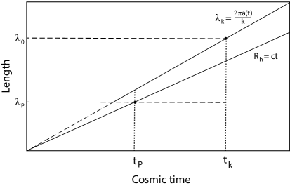
Figure 1: Schematic diagram illustrating a $k$-mode born across the Planck region and emerging into the semi-classical universe when its wavelength $\lambda_{k}$ equals the scale $\lambda_{0}$. The vertical axis shows proper distances as a function of cosmic time $t$ (increasing to the right on the horizontal axis). The time of birth $t_{k}$ is defined by the condition $\lambda_{0}=2\pi a(t_{k})/k$. In the $R_{\rm h}=ct$ cosmology, the ratio $\lambda_{k}/R_{h}$ is constant for all time $t$.

In the $R_{\rm h}=ct$ cosmology, we have several good reasons for adopting Hollands and Wald’s central idea. Chief among them is the empirical evidence described above, which supports the conclusion that $10^{\circ}$-anisotropies in the CMB would have had a size $\sim\lambda_{\rm P}$ at $\sim t_{\rm P}$ (see Table 1). Second, the very notion of a Planck length rests on the physical limitations imposed on the localization of a defined mass by its Compton wavelength $\lambda_{\rm C}$. Since the gravitational radius $R_{\rm h}(t)$ defines the maximum size of any causally connected region at time $t$ in this model [82, 83, 84], only proper masses smaller than $\sim R_{\rm h}/2G$ have any physical meaning. So quantum mechanical “fuzziness” extends over a scale $\sim\lambda_{\rm C}(t)=\lambda_{\rm P}^{2}/t$, even bigger than $\lambda_{\rm P}$ at $t<t_{\rm P}$.

As is well known from our experience with fluctuations in the inflaton field, and as evident in the form of the frequency $\alpha_{k}$ in Equation (32), modes with $\lambda_{k}<2\pi R_{\rm h}$ oscillate, while those with $\lambda_{k}>2\pi R_{\rm h}$ are effectively “frozen” on super-horizon scales (see discussion in § 1). And as one finds during inflation, the amplitude of the oscillating metric perturbation modes would have decayed too quickly for them to be observationally relevant at time $t_{\rm cmb}$. So we follow Hollands & Wald (2002) in identifying the Sachs-Wolfe perturbations in the CMB with those trans-Planckian fluctuations with super-horizon wavelengths at the time they were born. Figure 1 shows the key scales relevant to this hypothesis, including the Planck wavelength $\lambda_{\rm P}=R_{\rm h}(t_{\rm P})$, and the wavelength $\lambda_{k}=2\pi a(t)/k$ of mode $k$. We emphasize again the key difference between the numen-field and inflaton fluctuations, in that the ratio $\lambda_{k}/R_{\rm h}$ is constant for the former, while it first increases and then decreases during inflation.

For these reasons, we adopt the view that all the $k$-modes of interest in the CMB satisfy the condition

$$k={2\pi\over\epsilon_{k}\,\lambda_{\rm P}}a(t_{\rm P})\;,$$ (38)

where $\epsilon_{k}\gtrsim 1$. They emerge into the semi-classical universe when their wavelength equals the scale $\lambda_{0}$, so that (with $a(t)=t/t_{0}$)

$$t_{k}=k{\lambda_{0}t_{0}\over 2\pi}\;.$$ (39)

An alternative way to write this is

$$t_{k}={\lambda_{0}\over\epsilon_{k}\,\lambda_{\rm P}}t_{\rm P}\;.$$ (40)

We now write Equation (32) using the approximate expansion

$$\alpha_{k}\approx k\left(1-{1\over(kt_{0})^{2}}\right)\;,$$ (41)

so that with the definition of $z$ in Equations (29) and (30), the metric perturbation $\Theta_{k}$ has an amplitude frozen at the birth time $t_{k}$, given by the expression (cf. ref. [77])

$$\left|\Theta_{k}\right|^{2} = \left.\left({H\over\dot{\phi}}\right)^{2}{1\over 2a(t)^{2}\alpha_{k}}\right|_{t_{k}}$$ (42)

$$\approx {2\pi^{2}\over k^{3}}{\lambda_{\rm P}^{2}\over\lambda_{0}^{2}}\left(1-{1\over 2(kt_{0})^{2}}\right)^{-1}\;.$$

The power spectrum for these curvature perturbations is given by the $k$-space weighted contribution of modes [3, 12, 80, 81], commonly written as

$$\mathcal{P}_{\Theta}(k)\equiv{k^{3}\over 2\pi^{2}}|\Theta_{k}|^{2}\;.$$ (43)

We can therefore confirm that the spectrum of numen scalar curvature perturbations is almost scale free, i.e., $\mathcal{P}_{\Theta}(k)\sim k^{0}$, as seen in the CMB fluctuations, but not exactly. The common way to quantify the deviation from scale-invariance is via the scalar spectral index, $n_{s}$, defined according to

$$n_{s}-1\equiv{d\,\ln\mathcal{P}_{\Theta}(k)\over d\,\ln k}\;.$$ (44)

From Equations (42-44), we find that

$$n_{s}\sim 1-{2\over 2(kt_{0})^{2}-1}\;.$$ (45)

As we noted earlier in this section, the observed index is $n_{s}=0.968\pm 0.006$ [23], suggesting that the actual power spectrum is only approximately scale free. The implication of this measurement for the numen-field fluctuations is that the slight deviation from a pure scale-free spectrum appears to be due to the difference $k-\alpha_{k}$ in Equation (32). Furthermore, as was the case for Hollands and Wald [77], we find that the correct amplitude of the fluctuations in the CMB is produced if we choose $\lambda_{0}$ to be of order $10^{5}\,\lambda_{\rm P}$, the grand unification scale.

Of course, the value of the ratio in Equation (45)—and therefore of the inferred scalar spectral index $n_{s}$—depends on the wavenumber $k$. So the numen fluctuation spectrum will have a weakly running spectral index. Though perhaps not as reliable as the index $n_{s}$ itself, Planck constrained its scale dependence $dn_{s}/d\ln k$ to have the value $-0.003\pm 0.007$, possibly negative, though consistent with zero (or even slightly positive). From Equation (45), we find that the numen field has

$${dn_{s}\over d\ln k}\sim{4(kt_{0})^{2}\over[2(kt_{0})^{2}-1]^{2}}\;,$$ (46)

a very small, though positive number. Future work will tell whether this difference is meaningful, or whether it is simply due to the fact that the analysis reported by Planck was carried out solely in the context of $\Lambda$CDM.

4.2 Tensor Perturbations

The tensor perturbations $h_{ij}$ are transverse ($\partial^{i}h_{ij}=0$) and trace-free ($\delta^{ij}h_{ij}=0$) and are automatically independent of coordinate gauge transformations. These represent gravitational waves evolving independently of linear matter perturbations, and are typically decomposed into eigenmodes $e_{ij}$ of the spatial Laplacian operator with comoving wavenumber $k$ and scalar amplitude $h(t)$, such that

$$h_{ij}(t,\vec{x})=h(t)\,e_{ij}^{(+,\hbox{$\times$})}(\vec{x})\;,$$ (47)

with two independent polarization states $+$ and $\times$.

In addition to decoupling completely from scalar perturbations and not providing any backreaction to the metric, gravity waves also satisfy sourceless equations when the energy-momentum tensor is diagonal, like that in Equation (8). With the definition $v_{k}(t)\equiv(m_{\rm P}/\sqrt{32\pi})ah_{k}(t)$ for the Fourier components $h_{k}(t)$ of $h$ (based on Equation 47 and our definition of the Planck mass $m_{\rm P}=G^{-1/2}$), it is easy to see that the mode equation for the tensor perturbations (analogous to Equation 31) is

$$v_{k}^{\prime\prime}+\alpha_{k}^{2}v_{k}=0\;,$$ (48)

with the same frequency $\alpha_{k}$ defined in Equation (32).

The fields $v_{k}$ and $u_{k}$ are considered to have similar attributes, notably, that both are canonically normalized, and that both ‘freeze’ when their wavelengths exceed the horizon scale. Therefore, we can immediately write down the expression equivalent to Equation (42) for the amplitude of $h_{k}$:

$$|h_{k}|^{2}={32\pi\over m_{\rm P}^{2}}\left.{1\over 2a^{2}\,\alpha_{k}}\right|_{\lambda_{0}^{T}}\;,$$ (49)

where $\lambda_{0}^{T}$ is the scale—analogous to $\lambda_{0}$ for the scalar perturbations—at which the tensor modes emerge into the semi-classical universe. And therefore since there are two independent tensor polarization states, the tensor power spectrum (analogous to Equation 43) is

$$\mathcal{P}_{T}(k) \equiv {2k^{3}\over 2\pi^{2}}|h_{k}|^{2}$$ (50)

$$= 16{\lambda_{\rm P}^{2}\over\lambda_{0}^{2}}\left(1-{1\over 2(kt_{0})^{2}}\right)^{-1}\;.$$

We are now in a position to examine the third observational signature typically associated with the idea of a quantum-fluctuation origin for the anisotropies in the CMB—the ratio of tensor to scalar power, which we may write as follows:

$$r\equiv{\mathcal{P}_{T}(k)\over\mathcal{P}_{\Theta}(k)}=16\left({\lambda_{0}\over\lambda_{0}^{T}}\right)^{2}\;.$$ (51)

Those familiar with the inflationary scenario will recognize that this expression is very similar to the result associated with an inflaton field, except that in that case the right-hand side of this expression is $16\epsilon$, in terms of the slow-roll parameter $\epsilon\equiv-\dot{H}/H^{2}$.

Because tensor modes would have decoupled completely from everything else, one does not know about these fluctuations (1) whether they were produced in the trans-Planckian region, (2) whether they emerged into the semi-classical universe at the same fixed length scale $\lambda_{0}$ as the scalar perturbations, or (3) whether they were even generated after the Planck time. If they did emerge at a fixed scale $\lambda_{0}^{T}$, they would likely have a near-scale free spectrum, like the curvature perturbations, but one could not predict their power relative to that of the scalar fluctuations without knowing something about the scale at which they emerged [77]. It may already be possible to eliminate the first possibility, since the scaling for $\Theta_{k}$ and $h_{k}$, through their definition in terms of the modes $u_{k}$ and $v_{k}$, would suggest a ratio of tensor to scalar power exceeding current upper limits. Indeed, if we adopt the value $r\lesssim 0.11$ as the most recent observational constraint, our model would require

$$\lambda_{0}^{T}\gtrsim 12\lambda_{0}\;,$$ (52)

meaning that any gravity waves generated in this picture would also have been produced at the GUT scale. In the case of inflation, the slow-roll parameter $\epsilon$ is a direct probe into the energy scale of the inflaton field, and it is generally understood that if $r\gtrsim 0.01$, then the inflaton potential has a value $V^{1/4}\sim(r/0.01)^{1/4}10^{16}$ GeV, which itself lies in the GUT energy range. In some ways, this convergence of ideas is rather promising for the quantum-perturbation model for the origin of fluctuations in the cosmic fluid, since it suggests that the physics (as we know it) of scalar fields in the early Universe is rather tightly constrained, and perhaps the simplest extensions to the standard model are on the horizon.

5 Conclusions

One of the strongest arguments in favor of the freeze-out mechanism during inflation is the coherence of the observed CMB fluctuations [85]. Curvature perturbations eventually source density fluctuations that evolve under the influence of gravity and pressure to produce the CMB inhomogeneities and subsequent large-scale structure. If one reasonably supposes that recombination happens instantaneously (at least in comparison to the evolutionary timescale), then fluctuations with different wavelengths influence the surface of last scattering at different phases in their oscillations. However, if all Fourier modes of a given wavenumber have the same phase, then they interfere coherently, resulting in a CMB spectrum with clearly defined peaks and troughs. Without this coherence, the various modes would all combine to produce white noise.

With inflation, all the mode phases are set when the fluctuations exit the horizon, which therefore remain coherent upon subsequent re-entry. Something very similar to this happens with the numen field, since all the scalar modes of a given wavenumber $k$ emerge into the semi-classical universe at the same scale $\lambda_{0}$ and, therefore, at the same time $t_{k}$. These modes are super-horizon and frozen during the subsequent expansion. They eventually source matter and radiation fluctuations with the same phase when the numen field decays into standard-model particles. So the mechanism for generating coherence of the numen modes is very similar to that of the inflaton field, though perhaps a little simpler since it requires fewer steps and is a natural extension of the wavenumber-dependence of the emergence of these modes, unlike those associated with the inflaton field, which are considered to have been born at arbitrarily early (pre-Planckian) times [78].

The suggestion is sometimes made that Planck-era physics may eventually be studied with the CMB. In the $R_{\rm h}=ct$ universe, this idea is more than mere speculation. Indeed, as we have shown in this paper, CMB fluctuation scales and amplitudes are preserved at the values they had as they emerged out of the Planck domain. In particular, the identification of the angular scale of the CMB inhomogeneities with the Planck length is a strong factor in favor of this cosmology, particularly since the Universe would have expanded by over 60 orders of magnitude between the Planck and recombination times. One cannot completely rule out a coincidence such as this, though the probability of its occurrence is extremely small. So the connection between the CMB and Planck scales is already clearly defined in $R_{\rm h}=ct$.

We have also seen that if matter in the early universe was dominated by a single scalar field, then its potential in this model is known precisely (and given in Equation 18). This result may motivate further exploration of Kaluza-Klein cosmologies, string theories, and supergravity, in which exponential potentials such as these are well justified. In concert with constraints imposed by CMB observations, particularly the value of the scalar spectral index $n_{s}$, there is therefore hope that new physics may emerge with relevance to the trans-Planckian domain.

References

References

- [1] Kolb E W and Turner M 1990 The Early universe (Addison-Wesley, Reading MA)
- [2] Linde A D 1990 Particle Physics and Inflationary Cosmology (Harwood, Chur, Switzerland)
- [3] Liddle ARD and Lyth K A 2000 Cosmological Inflation and Large-Scale Structure (Cambridge University Press, Cambridge, England)
- [4] Kazanas D 1980 Astrophys J Lett 241 L59
- [5] Starobinsky A A 1980 Phys Lett 91B 99
- [6] Guth A H 1981 Phys Rev D 23 347
- [7] Sato K 1981 MNRAS 195 467
- [8] Sato K 1981 Phys Lett 99B 66
- [9] Turner M 2008 Nature Physics 4 89
- [10] Riotto A 2002 e-print (arXiv:hep-ph/0210162)
- [11] Martin J 2005 Lect Notes Phys 669 199
- [12] Bassett B A Tsujikawa S and Wands D 2006 Rev Mod Phys 78 537
- [13] Kinney W H 2009 TASI Lectures on Inflation (arXiv:0902.1529)
- [14] Sriramkumar L 2009 Curr Sci 97 868
- [15] Baumann D 2009 TASI Lectures on Inflation (arXiv:0907.5424)
- [16] Mukahnov V F and Chibisov G V 1981 JETP Lett 33 532
- [17] Guth A H and Pi S Y 1982 Phys Rev Lett 49 1110
- [18] Hawking S W 1982 Phys Lett B 115B 295
- [19] Starobinsky A A 1982 Phys Lett B 117B 175
- [20] Wright E L Bennett C L Gorski K Hinshaw G and Smoot G F 1996 Astrophys J Lett 464 L21
- [21] Bennett C L et al. 2013 Astrophys J Supp 208 id 20
- [22] Copi C J Huterer D Schwarz D J Starkman G D 2009 MNRAS 399 295
- [23] Ade PAR et al. 2015 A&A submitted (arXiv:1502.02114)
- [24] Copi C J Huterer D Schwarz D J and Starkman G D 2013 MNRAS in press (arXiv:1310.3831)
- [25] Melia F 2007 MNRAS 382 1917
- [26] Melia F and Shevchuk ASH 2012 MNRAS 419 2579
- [27] Melia F 2012 Australian Phys 49 83
- [28] Melia F 2014 A&A 561 id A80
- [29] Alcock C and Paczyński B 1979 Nature 281 358
- [30] Anderson L et al. 2014 MNRAS 441 24
- [31] Delubac T et al. 2015 A&A 574 A59
- [32] Melia F López-Corredoira M 2015 Proc R Soc A (arXiv:1503.05052)
- [33] Melia F 2013 A&A 553 id A76
- [34] Bengochea G R Canate P Sudarsky D 2015 PLB 743 484
- [35] Perez A Sahlmann H Sudarsky D 2006, CQG 23 2317
- [36] Khoury J Ovrut B A Steinhardt P J Turok N 2001 Phys Rev D 64 123522
- [37] Steinhardt P J Turok N 2002 Science 296 1436
- [38] Steinhardt P J 2004 Mod Phys Let A 19 976
- [39] Weyl H 1923 Z Phys 24, 230
- [40] Melia F and Abdelqader M 2009 Int J Mod Phys 18 1889
- [41] Misner C W and Sharp D H 1964 Phys Rev 136 571
- [42] Melia F 2013 Astrophys J 764 72
- [43] Melia F and Maier R S 2013 MNRAS 432 2669
- [44] Wei J J Wu X and Melia F 2013 Astrophys J 772 id 43
- [45] Melia F 2014 JCAP 01 027
- [46] Wei J J Wu Melia F Wei D M and Feng L L 2014 MNRAS 439 3329
- [47] Melia F 2014 Astron J 147 120
- [48] Wei J J Wu X and Melia F 2014 Astrophys J 788 id 190
- [49] Melia F Wei J J and Wu X 2015 Astron J 149 2
- [50] Wei J J Wu X and Melia F 2015 MNRAS 447 479
- [51] Melia F 2015 Astron J 149 6
- [52] Wei J J Wu X Melia F and Maier R S 2015 Astron J 149 102
- [53] Wei J J Wu X and Melia F 2015 Astron J 149 65
- [54] Wei J J Wu X Melia F Wang F Y and Hai Y 2015 Astron J 150 35
- [55] Melia F and McClintock T M 2015 Astron J in press (arXiv:1507.08279)
- [56] Melia F 2015 Astrophys & Space Sci 359 34
- [57] Melia F 2015 Astrophys & Space Sci 356 393
- [58] de Sitter W 1917 Proc Akad Wetensch Amsterdam 19 1217
- [59] Lyth D H and Riotto A 1999 Phys Rep 314 1
- [60] Lidsey J E Wands D and Copeland E J 2000 Phys Rep 337 343
- [61] Abbott L F and Wise M B 1984 Nucl Phys B244 541
- [62] Lucchin F and Matarrese S 1985 Phys Rev D 32 1316
- [63] Barrow J 1987 Phys Lett B 187 12
- [64] Liddle A R 1989 Phys Lett B 220 502
- [65] Tsujikawa S (2000) Phys Rev D 62 4
- [66] del Campo S Gonzalez C and Herrera R 2015 Astrophys & Space Sci 358 id 8
- [67] Starobinksy A A 1979 JETP Lett 30 682
- [68] Starobinksy A A 1985 Soviet Astron Lett 11 323
- [69] Bardeen J M 1980 Phys Rev D 22 1882
- [70] Kodama H Sasaki M 1984 Prog Theoretical Phys Supp 78 1
- [71] Mukhanov V F Feldman H A Brandenberger R H 1992 Phys Rep 215 203
- [72] Sasaki M 1986 Prog Theor Phys 76 1036
- [73] Mukhanov V F 1988 JETP 67 1297
- [74] Bunch T S and Davies PCW 1978 Proc R Soc A 360 117
- [75] Martin J and Brandenberger R 2001 Phys Rev D 63 123501
- [76] Sachs R K and Wolfe A M 1967 Astrophys J 147 73
- [77] Hollands S Wald R M 2002 Gen Rel Grav 34 2043
- [78] Brandenberger R and Ho P M 2002 Phys Rev D 66 023517
- [79] Hassan S F and Sloth M S 2003 Nucl Phys B674 434
- [80] Lidsey J E et al. 1997 Rev Mod Phys 69 373
- [81] Peiris H V et al. 2003 Astrophys J Supp 148 213
- [82] Bikwa O Melia F and Shevchuk ASH 2012 MNRAS 421 3356
- [83] Melia F 2012 JCAP 09 029
- [84] Melia F 2013 CQG 30 155007
- [85] Dodelson S 2003 AIP Conference Proceedings 689 184